Machine Learning Regression for Operator Dynamics

Abstract

Determining the dynamics of the expectation values of operators acting on quantum many-body systems is a challenging task. Matrix product states (MPS) have traditionally been the ”go-to” models for these systems because calculating expectation values in this representation can be done with relative simplicity and high accuracy. However, such calculations can become computationally costly when extended to long times. Here, we present a solution for efficiently extending the computation of expectation values to long time intervals. We utilize a multi-layer perceptron (MLP) model as a tool for regression on MPS expectation values calculated within the regime of short time intervals. With this model, the computational cost of generating long-time dynamics is significantly reduced, while maintaining a high accuracy. These results are demonstrated with operators relevant to quantum spin models in one spatial dimension.

I Introduction

The accurate determination of expectation values for operators acting on quantum many-body (QMB) systems at long times remains an open problem. Much progress has been made for various specific systems of interest, such as the Ising chain with a quenched transverse field,Calabrese2011 or the Ohmic spin-boson model coupled to a harmonic non-Markovian environment.Strathearn2018 However, these developments have focused on systems where symmetries and approximations can be exploited, analytic or exact diagonalization methods can be used, or matrix product state algorithms can be employed. Such approaches are either limited in their scope or quickly become computationally demanding, particularly for systems in more than one spatial dimension. This is particularly true for the standard time-evolving block decimation (TEBD) Paeckel2019 , time-dependent density matrix renormalization group ($t$-DMRG),Vidal2004 and dynamic density matrix renormalization group (DDMRG) algorithms.Jeckelmann2002

Recent advances in machine learning models have offered new insights and paved new pathways for modeling QMB systems, often providing significant computational advantages over traditional methods.Marcello2019 ; Melkinov2019 ; Soto2019 Motivated by these successes, we investigate the advantages machine learning can provide when computing the expectation values for operators acting on QMB systems within the long-time regime.

Previous work utilizing machine learning techniques in QMB systems was heavily focused on the use of restricted Boltzmann machines (RBMs) as generative models of quantum states.Nomura2017 ; Gao2017 ; Glasser2018 These are energy-based models with an energy cost function given by

$$E(v,h)=-\sum_{i}{a_{i}v_{i}}-\sum_{j}{b_{j}h_{j}}-\sum_{i,j}{v_{i}W_{ij}h_{j}}.$$ (1)

Here, $v=\{v_{i}\}$ and $h=\{h_{j}\}$ are the visible and hidden layers of neurons in the RBM network, respectively. Each visible (hidden) neuron can only take on the values $\pm 1$ with an associated bias $a_{i}$ ($b_{j}$) and is fully connected to the hidden (visible) layer by the weight matrix $W$.Montufar2018 Given a spin-1/2 system, the probability amplitude of a specific spin state, $\Psi_{\mathrm{RBM}}(v)$, can be represented by the RBM by setting a spin configuration $v$ for the visible layer and performing a summation over all hidden variables as

$$\Psi_{\mathrm{RBM}}(v) = \sum_{h}{e^{-E(v,h)}}$$ (2)

$$= \prod_{i}{e^{a_{i}v_{i}}}\prod_{j}{1+e^{b_{j}+\sum_{i}v_{i}W_{ij}}}.$$ (3)

To obtain information about the full state of the system, it is necessary to perform sampling over numerous spin configurations. While this model is preferably suited to the determination of ground state properties, after some modifications it has also been used to determine dynamical properties of QMB systems.Hartmann2019 ; Carleo2017 ; Hendry2019 Recently, convolutional neural network have also been used to map input QMB spin configurations to probability amplitudes.Schmitt2020 In spite of the success of these approaches, these models still face similar challenges as other computational methods, namely that accurately representing the system state becomes computationally demanding as the system size grows.

To circumvent the computational demands of representing (or sampling) the full state of the system at any given time, we focus our attention on the direct evolution of expectation values by breaking time into two domains. For any given operator $\mathcal{O}$ acting on a quantum system $\ket{\mathbf{\Psi}(t)}$, the expectation value of the operator at any given time is given by

$$\langle\mathcal{O}\rangle=\bra{\mathbf{\Psi}(t)}\mathcal{O}\ket{\mathbf{\Psi}(t)}.$$ (4)

By computing $\langle\mathcal{O}\rangle$ using matrix product state (MPS) algorithms within the short-time domain, we shown that the long-time expectation values can be determined with low computational effort and good accuracy by utilizing a multi-layer perceptron (MLP) as a tool for linear regression. It is noted that previous extrapolation methods have been studied, but these have either focused on constructing the wave function at each increment of time Tian2020 or implementing linear prediction methods to $t$-DMRG spectral calculations.Barthel2009

This paper is organized as follows: In Sec. II, we review the fundamentals of the multi-layer perceptron (MLP) model. In Sec. III, as a benchmark for algorithmic comparison, we review the time-evolving block decimation algorithm in the context of calculating operator dynamics. In Sec. IV, we describe the methodology involved in using the MLP for regression. In Sec. V, we demonstrate the computational advantage gained by using MLP regression to determine operator dynamics for both the Ising and the XXZ model. Finally, in Sec. VI, we interpret these results and provide a framework for further improvement and investigation.

II Multi-layer Perceptrons

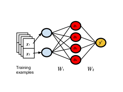
Figure 1: A graphical representation of an example MLP, with input vectors $\vec{x}_{n}$ each having two elements for use as input to the first layer of neurons (blue). This input is propagated to the next layer (red) by interconnecting weights $W_{1}$ and finally sent to the output (yellow) with weights $W_{2}$.

II.1 Architecture

In machine learning, the MLP model is a ubiquitous tool for performing classification tasks.Gardner1998 It is an input-output model approximating the function

$$y^{\prime}=W\cdot f(\mathbf{x}),$$ (5)

where $f(\mathbf{x})$ is an activation function over a set of inputs $\mathbf{x}$, $W$ is a weight matrix, and $y^{\prime}$ is a guessed classification label. This model is composed of $l$ sequential layers of neurons $\{a^{(i)}_{n_{i}}\}$, where $0<i<l$, and $n_{i}$ specifies the number of neurons in a given layer $i$. Each neuron is subject to the activation function $f$. Additionally, each layer of neurons has a specified weight matrix $W^{(i)}$, which connects the output from one layer to the input of the next. The components of each $W^{(i)}$ are used as parameters for optimization of the network.Gardner1998 Figure 1 provides a schematic for a MLP with a single layer of neurons between the input and final output.

II.2 Supervised Learning

To minimize the cost of the guessed label $y^{\prime}$ generated by the MLP, we provide an initial data set having $N$ elements, $\{\mathbf{x}_{n},y_{n}\}$, where $0<n<N$, for use in a training protocol. This provision for training is characteristic of supervised learning.Kotsiantis2007 In this learning procedure, each input vector $\mathbf{x}_{n}$ is accompanied by a corresponding true classification label $y_{n}$. This label provides the reference for a cost function $C(y_{n}^{\prime},y_{n})$ which measures the distance between the current MLP output classification label $y_{n}^{\prime}$ and the true classification label $y_{n}$.Kotsiantis2007 For our specific purposes,xs we define $C(y_{n}^{\prime},y_{n})$ as

$$C(y_{n}^{\prime},y_{n})=\frac{1}{N}\sum_{n}^{N}|y_{n}^{\prime}-y_{n}|.$$ (6)

Minimizing this cost function can be accomplished by any selection of known optimizations algorithms. For our purposes, we focus on using a stochastic gradient descent method.Zhang2004

III Time Evolving Block Decimation

Before introducing the MLP regression algorithm, we provide a short review of the TEBD algorithm so that computational comparisons to our algorithm might be well understood. The TEBD algorithm facilitates the time evolution (real or imaginary) of one-dimensional quantum systems under local Hamiltonians.Paeckel2019 As such, it is naturally expressed within the framework of matrix product states (MPS). The time evolution is accomplished by generating and repeatedly applying Suzuki-Trotter expansions of the time evolution operator $\exp{(-i\mathcal{H}T)}$, up to any specified order. Given a Hamiltonian with nearest-neighbor interactions and open boundary conditions (OBC) over $N$ sites,

$$\mathcal{H}=\sum_{i=1}^{N-1}H_{i,i+1},$$ (7)

the second-order Suzuki-Trotter expansion of $\exp{(-i\mathcal{H}T)}$ for a small time-step $\delta>0$ is given as

$$e^{-iT\mathcal{H}} \approx \left[(e^{-\frac{i\delta}{2}H_{1,2}}e^{-\frac{i\delta}{2}H_{3,4}}\cdots e^{-\frac{i\delta}{2}H_{n-1,n}})\right.$$ (8)

$$\left.\times\ (e^{-i\delta H_{2,3}}e^{-i\delta H_{4,5}}\cdots e^{-i\delta H_{n-2,n-1}})\right.$$

$$\left.\times\ (e^{-\frac{i\delta}{2}H_{1,2}}e^{-\frac{i\delta}{2}H_{3,4}}\cdots e^{-\frac{i\delta}{2}H_{n-1,n}})\right]^{T/\delta}.$$

The sequential application of these operators demands that the MPS be brought to canonical form (i.e., orthonormalizing the indices) after every time step $\delta$.Vidal2004 Such a procedure involves $O(poly(N)poly(D))$ steps, where $D$ is the maximum internal bond dimension of the MPS. In the absence of truncation, $D$ grows exponentially with both the system size and the evolution time and the computational cost of this procedure quickly becomes intractable for large systems and long times.

After the application of these operators, the final state of the system is obtained as

$$\ket{\Psi(t=T)}=e^{-iT\mathcal{H}}\ket{\Psi(t=0)}.$$ (9)

Typically, there are two sources of error in the TEBD framework. The first comes from the truncation of the MPS bond dimensions during the orthonormalization process. The other source of error arises during the Suzuki-Trotter expansion, which for our purposes is taken to second order. In this case, the error per time step is on the order $O(\delta^{3})$ resulting in an error over the total time interval on the order of $O(\delta^{2})$. In this paper, we choose to mitigate the first source of error by performing minimal amounts of truncation on the MPS (i.e., maintaining large bond dimensions). This is done to ensure that the primary source of error arises from the Trotter-Suzuki approximation itself.

IV Machine Learning Regression

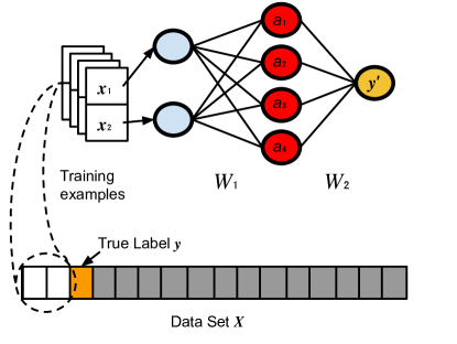
Figure 2: An example diagram for MLP regression. The input data set $X$ is decomposed into sets of training examples consisting of input vectors (white) and output values (yellow) selected from contiguous blocks in $X$. These training examples are fed into the MLP as shown.

In order to effectively model the evolution of operator expectation values, we construct the MLP in a manner conducive to regression rather than classification. Accomplishing this involves a few specifications about the input-output pairs $\{\mathbf{x},y\}$. We treat an input vector $\mathbf{X}$ as being parameterized by time $t$ over a time interval $[0,\tau]$ so that each element $X_{i}\in\mathbf{X}$ is labeled by a coordinate $t_{i}$. The total time $\tau$ is partitioned into $m$ discrete time intervals $\{t_{i}|0<i<m\}$. From $\mathbf{X}$, each input-output pair is constructed as follows. Starting from the first element in $\mathbf{X}$ corresponding to time $t_{0}=0$, we select a contiguous block of $p$ elements from $\mathbf{X}$ to form an input vector $\mathbf{x}=\{X_{0},X_{1},...,X_{p}\}$. We call this block our training window. The corresponding label for this window is selected as the element $X_{p+1}$. To construct multiple input examples for training, we shift the starting position of the training window throughout $\mathbf{X}$ until the desired number of examples is achieved. A diagram of this initialization procedure is given in Fig. 2.

In addition to constructing the input-output pairs in the aforementioned manner, we choose to define our activation functions by the linear unit, $f=x$. This activation allows us to effectively propagate all of the input information through the network. This is in contrast to the more commonly used rectified linear unit (ReLU), $f=\max(0,x)$, which, depending on the values selected for the weights, can suppress some information propagation through the network by eliminating all negative values.Nwankpa2018 The ReLU activation is useful when the MLP is used for classification over a discrete set of positive valued labels. However, we select the linear activation because our output values are continuous and include values less than zero.

V Results

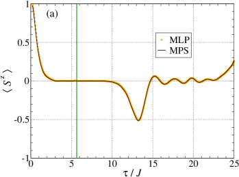
(a)

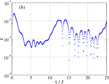
(b)

Figure 3: (a) Time evolution of the expectation value $\langle S^{z}\rangle$ up to $\tau=25/J$ in time steps of $\delta=0.05/J$ for the one-dimensional Ising spin chain with $N=12$ sites, exchange coupling $J$, and transverse field $\Delta=J$ (i.e., at the critical point). The MLP used for the regression was constructed with 32 linear activated neurons using a training window size of $p=4$. The selection of training examples employs the first 110 time steps (left of the green line). Results for the MLP regression are compared to TEBD results with maximum bond dimension $D=200$. (b) The absolute difference $\epsilon=|\langle S^{z}_{\mathrm{MPS}}\rangle-\langle S^{z}_{\mathrm{MLP}}\rangle|$ between the TEBD and the MLP regression is shown for each time step.

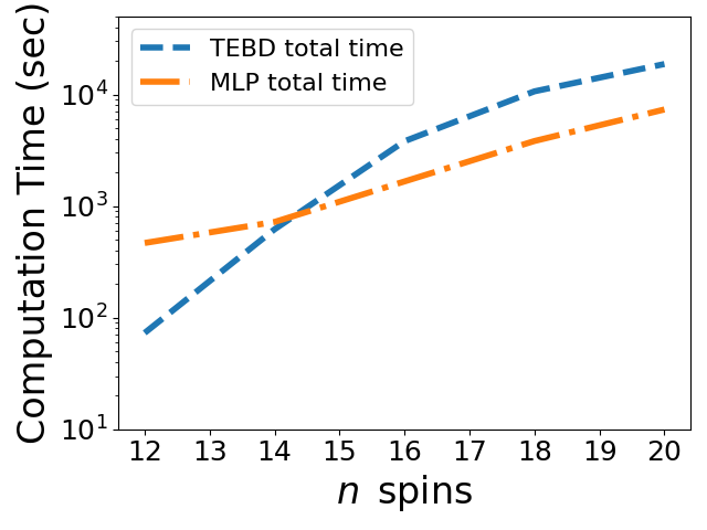
Figure 4: A comparison between the total computational times for the TEBD and the MLP regression algorithms. Each method was used to determine the dynamics of the expectation value of the $S^{z}$ operator for the transverse-field Ising model with exchange coupling $J$, transverse field, $h=J$, and evolution time $\tau=25/J$ in increments of $\delta=0.05/J$. The MLP regression was trained by stochastic gradient descent over 32 linearly activated neurons, regardless of size. For the TEBD, the maximal bond dimension was set to $D=200$ for all sizes.

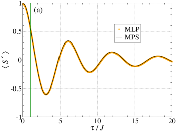
(a)

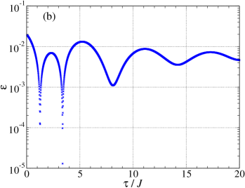
(b)

Figure 5: (a) Time evolution of the expectation value $\langle S^{z}\rangle$ up to $\tau=20/J$ in times steps of $\delta=0.01/J$ for the one-dimensional spin 1/2 XXZ chain with $N=12$ sites, $\Delta=J/2$, and $h=J/2$. The MLP used for the regression was constructed with 64 linear activated neurons using a training window size of $p=4$. The selection of training examples come only from the first 100 time steps (green line). Results for the MLP regression are compared with TEBD results without bond truncation (i.e., exact). (b) The absolute difference $\epsilon=|\langle S^{z}_{\mathrm{MPS}}\rangle-\langle S^{z}_{\mathrm{MLP}}\rangle|$ between TEBD calculations and the MLP regression are shown for each time step.

We test our MLP regression by evaluating operator expectation values over two model systems and comparing them to second-order Trotter-Suzuki time evolved MPS calculations. Firstly, we determine values at the critical point for the one-dimensional Ising model in a transverse field with an evolution time of $\tau=25/J$, where $J$ is the exchange coupling constant. To compare the computational cost between the TEBD and the MLP regression, we measure the computational time as a function of system size. Secondly, we apply the MLP regression to the one-dimensional XXZ model as a demonstration of its adaptability to various models. All machine learning simulations were implemented using the Tensorflow Keras library.chollet2015

V.1 Ising Model

For $N$ spins in a one-dimensional chain, the nearest-neighbor Ising model in the presence of a transverse field is given by the Hamiltonian

$$\mathcal{H}=-J\sum_{i=1}^{N-1}S^{z}_{i}\,S^{z}_{i+1}-h\sum_{i=}^{N}S^{x}_{i},$$ (10)

where $S^{z}$ is the longitudinal spin operator, $J$ is the exchange coupling constant, and $h$ characterizes the strength of the transverse field. Due to the non-commutability of terms in the Hamiltonian, this model is known to have a quantum phase transition at $J=h$ in one spatial dimension. This phase transition takes the system from the ordered ferromagnetic state to a paramagnetic state.Strecka2015

As an illustration of our method, we investigate the dynamics of the expectation of the local spin operator $\langle S^{z}\rangle$ near this phase transition for a short spin chain with $N=12$ spins. We first use calculations obtained from an MPS with OBC initialized in the ferromagnetic state to generate expectation values for time steps of $\delta=0.05/J$. We split these time-ordered expectation values into subsets for training and testing the MLP. For our model, we select training windows of $p=4$, giving us access to 995 input-output pairs. Of this, we use 110 pairs for training. Our MLP architecture is optimized with the following parameters: one layer of 32 linear activated neurons, followed by a single layer with one linear activated neuron for output. Training is carried out by a stochastic gradient descent over the cost function given in Eq. (6). Figure 3 shows the results with $h=J$ and maximal bond dimension $D=200$. Within the training region, the MLP is trained until it has significant overlap with the MPS calculations. This overlap is seen to continue far past the region of training. Comparison with the MPS results, as shown in Fig. 3(b), reveal that the MLP deviates from the MPS calculations with an average absolute deviation $\epsilon=|\langle S^{z}_{\mathrm{MPS}}\rangle-\langle S^{z}_{\mathrm{MLP}}\rangle|$ equal to $3\times 10^{-3}$. We note that the training time and parameters were selected in such a way as to mitigate overfitting for the given number of training examples, which explains why the deviation is relatively high in the training range. Using a standard desktop computer, the time to train the MLP was 415.24 seconds, while the time to predict the rest of the dynamics was 35.87 seconds. Comparatively, at this system size, exact diagonalization calculations took approximately 60 seconds, and TEBD calculations (with fixed bond dimension $D=200$) took approximately 0.146 seconds per time step, resulting in a total computation time of 73 seconds.

To glean information about the scaling of the computational cost of our approach (demonstrating its advantage for larger systems), we measure the time required to generate short-time TEBD expectation values as input data and add this to the computational time required for training and predicting in the long-time regime for varying system sizes $N$. This computation time is compared to the total time taken by the TEBD to calculate expectation values over the full time interval $\tau=25/J$. Figure 4 displays this comparison. It is clear that the scaling of the computational time is more favorable for our method. Still, a more interesting result appears if the time required for generating the input data is excluded. As shown in Table 1, within this regime of system sizes (having trained until an average deviation of $\epsilon=10^{-3}$ is achieved), the scaling of the overall computational time for the MLP regression is due primarily to the time necessary to generate input-output training pairs. The computational time necessary for the training and prediction steps in the algorithm appears polynomial (nearly linear), being primarily due to the necessary increase in the number of training required to maintain the given deviation $\epsilon$.

System size	Number of Training Sets Needed	Training Set Generation	Training + Prediction
($N$)	($N_{\rm train}$)	(seconds)	(seconds)
12	110	16.06	451.11
14	120	148.8	572.47
16	140	1,069.32	594.62
18	150	3,205.5	626.69
20	175	6,562.5	783.55

Table 1: Dependence of computational times on systems sizes for the transverse-field Ising model. The second column shows the number of training examples generated to maintain an average deviation $\epsilon=10^{-3}$. The third column shows the computational times to generate the training set of TEBD expectation values. The fourth column shows the computational times required for the training and predicting stages of the MLP regression.

V.2 XXZ Model

We test another ubiquitous spin system with our MLP regression, namely, the XXZ model. The Hamiltonian governing the evolution of this open boundary system is given by

$$\mathcal{H} = -J\sum_{i=1}^{N-1}\left(S^{x}_{i}S^{x}_{i+1}+S^{y}_{i}S^{y}_{i+1}+\Delta\,S^{z}_{i}S^{z}_{i+1}\right)$$ (11)

$$-\ h\sum_{i=1}^{N}S^{x}_{i},$$

where $J$ and $\Delta$ control the strength of the exchange coupling and the uniaxial anisotropy, respectively, and $h$ is the strength of transverse field. The transverse and longitudinal exchange couplings are $J_{\perp}=J$ and $J_{z}=J\,\Delta$, respectively. Similar to the Ising model above, the XXZ model exhibits transitions between the paramagnetic and the ferromagnetic phases ($J>0$), with critical values at $h_{c}=\pm(J_{\perp}-J_{z})=J(1-\Delta)$.Franchini2017 We investigate this model for $N=12$ spins and $\Delta=h=J/2$ (within the paramagnetic phase). Initially, the system is set at the fully-polarized ferromagnetic state.

We again select a training window of $p=4$, producing 1995 input-output pairs. From these, we train over 100 pairs. The MLP is composed of a single layer of 64 linearly activated neurons, followed by an output layer with a single linearly activated neuron. This model is again trained used stochastic gradient descent. Comparing with the results taken from MPS calculations over time intervals $\delta=0.01$, we see in Fig. 5 that the MLP regression agrees with the MPS and continues to do so deep into the testing regime. As shown in Fig. 5(b), the MLP on average differs consistently from the TEBD calculations by an average absolute differnce equal to $6\times 10^{-3}$. The time to sufficiently train to the desired accuracy was 200.99 seconds, while the time to predict the rest of the dynamics was 150.14 seconds. Comparatively, exact diagonalization calculations took approximately 60 seconds, and TEBD calculations took approximately 300 seconds per time step at the maximal bond dimension, for a total computation time of approximately 166.67 hours. As for the case of the Ising model, for such a small system, exact diagonalization is the most cost effective method for computing $\langle S^{z}\rangle$, but the cost of this method increases exponentially with system size as $O(2^{3N})$. As previously shown in Table 1, the scaling is more favorable for MLP.

VI Discussion

By investigating the evolution of the expectation value of operators, we have demonstrated that MLP regression accurately extends calculations in a highly reduced parameter space using very few training examples. To understand the significance of this, a comparison between the computational resources used in TEBD and MLP calculations is presented. For TEBD calculations, long-time dynamics are obtained by determining the state of the system $\ket{\Psi_{\mathrm{MPS}}}$ at every time step.Paeckel2019 For $N$ sites with maximal bond dimension $D$, this results in using $O(poly(N)poly(D))$ steps, more specifically, $O(2w^{3}ND^{3})$ steps for the sequential application of one- and two-body operators, where $w$ is the matrix dimension of the applied local operator.Orus2014 Computations with this complexity quickly become cumbersome for long times, particularly when the correlation length of the system diverges and the bond dimension $D$ scales exponentially. However, the MLP regression circumvents this computational cost by utilizing a small fixed ”memory” of previously generated expectation values as the basis for extending calculations out to long times. As can be seen in Table 1, the computational cost of the combined training and prediction steps of the regression is approximately polynomial. To understand how this short ”memory” reduces the complexity, consider a training set having $N_{\mathrm{train}}$ examples constructed over training windows (i.e., ”memories”) of size $p$ input into a neural network have $m$ neurons. For a given value of $p$ elements, the training phase of the MLP regression has a computational cost which is determined entirely by the neural network model parameters, $O(m^{2}p^{2}N_{\mathrm{train}})$. After the training, prediction for later times only has a computational cost of $O(1)$. By generating the first few expectation values with the MPS, the MLP regression is shown to be able to predict long-time operator expectations values with only the addition of a relatively small number of compute cycles. We conclude that within the regime of sizes considered in this study, the computational cost of the MLP regression scales remarkably slowly (nearly constant).

Though this computational advantage is significant, it is worth noting that the MLP regression can only extend the operator expectation values generated by the MPS. It is not a generative model and therefore cannot calculate operator dynamics without the presence of some initial expectation values. Further work must be done to explore machine learning architectures which can directly generate operator dynamics while maintaining low computational costs. Nonetheless, the results of this work indicate that machine learning techniques continue to provide unforeseen advantages in modeling QMB systems.

References

- (1) P. Calabrese, F. H. L. Essler, and M. Fagotti, Quantum quench in the transverse field ising chain, Phys. Rev. Lett. 106, 227203 (2011).
- (2) A. Strathearn, P. Kirton, D. Kilda, J. Keeling, and B. W. Lovett, Efficient non-markovian quantum dynamics using time-evolving matrix product operators, Nature Commun. 9, 3322 (2018).
- (3) S. Paeckel, T. Köhler, A. Swoboda, S.R. Manmana, U. Schollwöck, and C. Hubig, Time-evolution methods for matrix-product states, Ann. Phys. 411, 167998 (2019).
- (4) G. Vidal Efficient simulation of one-dimensional quantum many-body systems, Phys. Rev. Lett. 93, 040502 (2004).
- (5) E. Jeckelmann, Dynamical density martix renormalization group method, Phys. Rev. B 66, 045114 (2002).
- (6) D. C. Marcello, M. Caccin, P. Baireuther, T. Hyart, and M. Fruchart Machine learning assisted measurement of local topological invariants, arXiv:1901.03346 (2019).
- (7) A. Melkinov, L. Fedichkin, and A. Alodjants, Predicting quantum advantage by quantum walk with convolutional neural networks, New J. Phys. 21, 125002 (2019).
- (8) K. Chinjo and S. Sota and S. Yunoki, and T. Tohyama Characterization of photoexcited state in the half-filled one-dimensional extended hubbard model assisted by machine learning, Phys. Rev. B 101, 195136 (2020).
- (9) Y. Nomura, A.S. Darmawan, Y. Yamaji, and M. Imada, Restricted boltzmann machine learning for solving strongly correlated quantum systems, Phys. Rev. B 96, 205152 (2017).
- (10) X. Gao and L-M. Duong, Efficient representation of quantum many body states with deep neural networks, Nat. Commun. 8, 662 (2017).
- (11) I. Glasser, N. Pancotti, M. August, I. D. Rodriguez, and J. I. Cirac, Neural-network quantum states, string-bond states, and chiral topological states, Phys. Rev. X 8, 011006 (2018).
- (12) G. Montufar, Restricted boltzmann machines: Introduction and review, arXiv:1806.07066 (2018).
- (13) M. J. Hartmann and G. Carleo, Neural network approach to dissipative quantum many-body dynamics, Phys. Rev. Lett. 122, 250502 (2019).
- (14) G. Carleo and M. Troyer, Solving the quantum many-body problem with artificial neural networks Science 355, 602 (2017).
- (15) D. Hendry and A. E. Feiguin, A machine learning approach to dynamical properties of quantum many-body systems, Phys. Rev. B 100, 245123 (2019).
- (16) M. Schmitt and M. Heyl, Quantum many-body dynamics in two dimensions with artificial neural networks, Phys. Rev. Lett. 125, 100503 (2020).
- (17) Y. Tian and S. R. White, Matrix product state recursion methods for strongly correlated quantum systems, arXiv:2010.00213 (2020).
- (18) T. Barthel, U. Schollwock and S. R. White, Spectral functions in one-dimensional quantum systems at T¿0, Phys. Rev. B. 79, 245101 (2009).
- (19) M.W. Gardner and S.R. Dorling, Artificial neural networks (the multilayer perceptron): A review of applications in the atmospheric sciences, Atmos. Environ. 32, 2627–2636 (1998).
- (20) S. B. Kotsiantis, Supervised machine learning: A review of classification techniques, Informatica 31, 249–268 (2007).
- (21) T. Zhang, Solving large scale linear problems using stochastic gradient descent algorithms, in Proccedings of the 21st International Conference on Machine Learning (2004).
- (22) C. Nwankpa, W. Ijomah, A. Gachagan, and S. Marshall, Activation functions: Comparison of trends in practice and research for deep learning, arXiv:1811.03378 (2018).
- (23) Keras https://keras.io
- (24) J. Strecka and M. Jascur, A brief account of the ising and ising-like models: Mean-field, effective-field and exact results, Acta Phys. Slovaca 65, 235–367 (2015).
- (25) F. Franchini An introduction to integrable techniques for one-dimensional quantum systems (Springer, 2017).
- (26) R. Orus, A practical introduction to tensor networks: Matrix product states and projected entangled pair states, Ann. Phys. 349, 117–158 (2014).