Phenomenological study of the anisotropic quark matter in the 2-flavor Nambu-Jona-Lasinio model

Abstract

With the two flavor Nambu-Jona-Lasinio (NJL) model we carry out a phenomenological study on the chiral phase structure, mesonic properties and transport properties in a momentum-space anisotropic quark matter. To calculate transport coefficients we have utilized the kinetic theory in the relaxation time approximation, where the momentum anisotropy is embedded in the estimation of both distribution function and the relaxation time. It is shown that an increase of the anisotropy parameter $\xi$ may results in a catalysis of chiral symmetry breaking. The critical endpoint (CEP) is shifted to smaller temperatures and larger quark chemical potentials as $\xi$ increases, the impact of momentum anisotropy on temperature of CEP is almost the same as that on the quark chemical potential of CEP. The meson masses and the associated decay widths also exhibit a significant $\xi$ dependence. It is observed that the temperature behavior of scaled shear viscosity $\eta/T^{3}$ and scaled electrical conductivity $\sigma_{el}/T$ exhibit a similar dip structure, with the minima of both $\eta/T^{3}$ and $\sigma_{el}/T$ shifting toward higher temperatures with increasing $\xi$. Furthermore, we demonstrate that the Seebeck coefficient $S$ decreases when temperature goes up and its sign is positive, indicating the dominant carriers for converting the temperature gradient to the electric field are up-quarks. The Seebeck coefficient $S$ is significantly enhanced with a large $\xi$ for the temperature below the critical temperature.

I introduction

The properties of strongly interacting matter described by the quantum chromodynamics (QCD) in extreme conditions of temperature $T$ and density have aroused a plethora of experimental and theoretical studies in the last thirty years. The experiment studies performed at the Relativistic Heavy Ion Collider (RHIC) in BNL and the Large Hadron Collider (LHC) in CERN have revealed that a new deconfined state of matter $-$ the quark-gluon plasma (QGP), can be created at high temperature and/or baryon chemical potential $\mu_{B}$. And lattice QCD calculation, which is a powerful gauge invariant approach to investigate the non-perturbative properties, also has confirmed that the phase transition is a smooth and continuous crossover for vanishing chemical potential Bazavov:2014pvz ; Aoki:2006we ; Borsanyi:2013bia ; Borsanyi:2010cj ; Bernard:2004je ; Aoki:2006br . Due to the so-called fermion sign problem Splittorff:2007ck , lattice QCD simulation is limited to low finite density Barducci:1989wi ; Asakawa:1989bq ; Bazavov:2018mes , eventhough several calculation techniques such as the Taylor expansion talor1 ; talor2 , analytic continuations from imaginary to real chemical potential imagnary1 ; imagnary2 , multi-parameter reweighting method Fodor:2001au have been proposed to tackle this problem and improve the validity at high chemical potential. More detailed review of lattice calculation can be found in Refs. lattice1 ; lattice2 . Therefore, for arbitrary $\mu_{B}$ one has to rely on effective models to study the QCD phase transition. Currently, there are various QCD inspired effective models such as the Nambu-Jona-Lasinio (NJL) model 3flavor-NJL ; NJL1 ; NJL2 ; Buballa:2003qv , the Polyakov-loop enhanced NJL (PNJL) model Ratti:2006wg ; Mukherjee:2006hq ; Costa:2010zw ; Fukushima:2008wg , the Quark-Meson (QM) model Schaefer:2006ds ; Schaefer:2008hk ; Tripolt:2013jra , the Polyakov QM (PQM) model PQM ; Skokov:2010wb ; Schaefer:2011ex , which not only can successfully describe the spontaneous symmetry breaking and restoration of QCD but also have been applied to explore QCD phase structure and internal properties of meson at arbitrary $T$ and $\mu_{B}$. And these models calculations have predicted (see e.g. Schaefer:2008hk ; Zhuang:1994dw ) that at high chemical potential, the phase transition is a first-order phase transition, and with decreasing $\mu_{B}$, the first-order phase transition has to end at a critical end point (CEP) and change into a crossover. At this CEP the phase transition is of second order. However, due to various approximation adopted in the model calculations, there is not an agreement on the existence and location of CEP on the phase diagram. Furthermore, the effects of rotation Zhang:2020hha ; Jiang:2016wvv , the magnetic field effects Gatto:2010pt ; Kashiwa:2011js ; DElia:2018xwo ; Andersen:2013swa ; Ferreira:2015jrm ; Bali:2011qj , finite-volume effects Wan:2020vaj ; Zhao:2019ruc ; Palhares:2009tf ; Liu:2020elq ; Xu:2020loz ; Magdy:2019frj ; XiaYongHui:2019gci ; Tripolt:2013zfa ; Bhattacharyya:2012rp ; Deb:2020qmx , non-extensive effects Zhao:2020wks ; Shen:2017etj ; Rozynek:2009zh ; Ishihara:2019ran , external electric fields Tavares:2019mvq ; Ruggieri:2016xww ; Cao:2015dya ; Ruggieri:2016lrn , and the effects of chiral chemical potential Shi:2020uyb ; Braguta:2016aov ; Yu:2015hym ; Lu:2016uwy also have been considered in the effective models to provide a better insight in the phase transition of the realistic QCD plasma.

Apart from the importance of QCD phase structure information, the transport coefficients, characterizing the non-equilibrium dynamical evolution of QCD matter, also have captured large attention. The shear viscosity $\eta$, which quantifies the rate of momentum transfer in the fluid with inhomogeneous flow velocity, has been successfully used in the viscous relativistic hydrodynamic description of the QGP bulk dynamics. The small shear viscosity to entropy density ratio $\eta/s$ can be exctrated from the elliptic flow data v2 . In the literature, there are various frameworks for estimating $\eta$ of strongly interacting matter, e.g., the kinetic theory within the relaxation time approximation (RTA), the QCD effective models Ghosh:2014vja ; Marty:2013ita ; shear-NJL ; shear-PNJL ; Zhuang:1995uf ; Rehberg:1996vd , the quasiparticle model (QPM) shear-quasi1 ; shear-quasi2 , lattice QCD simulation shear-Lattice5 , ect. The electrical conductivity $\sigma_{el}$, as the response of a medium to an applied electric field, also has attracted more attention in high energy physics due to the presence of strong electromagnetic field created in the early stage of non-central heavy-ion collisions (HICs). The presence of $\sigma_{el}$ not only can affect the duration and strength of magnetic fields McLerran:2013hla ; Gursoy:2014aka , but also is directly proportional to the emissivity and production of soft photon Gupta:2003zh ; Yin:2013kya . The thermal behavior of $\sigma_{el}$ has been estimated using different approaches, such as the microscopic transport models Hammelmann:2018ath ; Steinert:2013fza ; Greif:2014oia ; electrical-phsd , lattice gauge theory simulation electrical-Lattice1 ; electrical-Lattice2 ; electrical-Lattice4 ; Amato:2013naa , hadron resonance gas model shear and electrical ; electrial2 ; electrical-EVHRG , quasiparticle models Mykhaylova:2020pfk ; Bluhm:2009ef , the effective models Marty:2013ita ; Soloveva:2020hpr , the string percolation model electrical-string1 ; electrical-string2 , the holographic method Jain:2010ip ; Finazzo:2013efa and so on. Recently, the studies of electrical conductivity in the QGP at magnetic fields have also been performed Thakur:2019bnf ; Kurian:2017yxj ; Rath:2020idp ; electrical1 ; Astrakhantsev:2019zkr . Another less concerned but interesting coefficient is Seebeck coefficient (or called thermopower). When a spatial gradient of temperature exists in a conducting medium, a corresponding electric field can arise and vice versa, which is the Seebeck effect. When the electric current induced by electric field can compensate with the current of temperature gradient, the thermal diffusion ends. Accordingly, the efficiency of converting temperature gradient to electric field in the open circuit condition is quantified by Seebeck coefficient $S$. In past years, the Seebeck effect has been extensively investigated in condensed matter physics. Very recently, some exploration has been extended to the QCD matter. For example, Seebeck coefficient at magnetic fields and at zero magnetic field has been studied in both the hadronic matter Das:2020beh ; Bhatt:2018ncr and the QGP Zhang:2020efz ; Dey:2020sbm ; Kurian:2021zyb . In Ref. Abhishek:2020wjm , Seebeck coefficient also has been estimated based the NJL model, where the spatial gradient of quark chemical potential is considered apart from the presence of temperature gradient.

In the beginning of HICs, the pressure gradient of created fireball along the beam direction (denoted as longitudinal $z$ direction) is greatly lower than along transverse direction. After the rapid expansion of medium along the beam direction, the system becomes much colder in the beam direction than the transverse direction Baier , which causes the QGP possess the local momentum anisotropy, and this anisotropy can survive in the entire evolution of medium Strickland:2014pga . In addition, the presence of strong magnetic field also can induce a local anisotropy in momentum-space.

Inspired by the presence of momentum-space anisotropy in HICs, the primary objective of present work is to study phenomenologically the effect of momentum anisotropy induced by the rapid longitudinal expansion of medium on the chiral phase structure, mesonic properties, and transport coefficients in the SU(2) NJL model. To incorporate momentum anisotropy into numerical calculations, we follow the parametrization method proposed by Romatschke and Strickland Romatschke:2003ms , where the isotropic momentum-space distribution functions of particle are deformed by rescaling one preferred direction in momentum space and introducing a directional dependent parameter $\xi$. This method has been extensively employed to phenomenologically study the impacts of momentum anisotropy on various observables, such as photon production Kasmaei:2019ofu ; Schenke:2006yp ; Bhattacharya:2015ada , the parton self-energy Kasmaei:2016apv ; Kasmaei:2018yrr ; Ghosh:2020sng , heavy-quark potential Nopoush:2017zbu ; Dumitru:2007hy , and various transport coefficients Thakur:2017hfc ; Rath:2019vvi ; Srivastava:2015via ; Baier:2008js . And the relativistic anisotropic hydrodynamics (aHydro) models can give a higher accurate description of non-equilibrium dynamics compared to other hydrodynamical models Alqahtani:2017mhy . As done in most previous studies, the present focus is on the weakly anisotropic medium (very close to the equilibrium) for which $|\xi|\ll 1$ and the distribution function can be expanded up to linear order in $\xi$. We can find that even at the small values of anisotropy, the effective quark mass and meson masses change significantly compared to the equilibrium result. Unlike most momentum anisotropy studies of transport coefficients in the QGP, where the effect of momentum anisotropy is not considered into the different particle interaction channels, in present work, we incorporate the momentum anisotropy to the estimation of the relaxation time to better study the impact of $\xi$ on transport properties of quark matter near the phase transition temperature region.

The paper is organized as follows: Sec. II gives a brief review of the basic formalism of the 2-flavor NJL model. In Sec. III and Sec. IV, we present the brief derivation of the expressions associated with the constituent quark mass and meson mass spectrum in an isotropic and anisotropic medium, respectively. Sec. V includes a detailed procedure for obtaining the formulae of momentum-anisotropy-dependent transport coefficients. In Sec. VI, we present the estimation of the relaxation time for (anti-)quarks. The numerical results for various observables are phenomenologically analyzed in Sec. VII. In Sec. VIII, the present work is summarized with an outlook. The formulae of the matrix elements squared for different quark-(anti-)quark elastic scattering processes are given in the Appendix.

II Theoretical frame

In this work, we start from the standard two-flavor NJL model, which is a purely fermionic theory due the absence of all gluonic degrees of freedom. Accordingly, the lagrangian is given as NJL1

$$\mathcal{L}=\bar{\psi}(i\not{\partial}-\hat{m}_{0})\psi+G[(\bar{\psi}\psi)^{2}+(\bar{\psi}i\gamma_{5}{\bf{\hat{\tau}}}\psi)^{2}],$$ (1)

where $\psi(\bar{\psi})$ stands for the quark (antiquark) field with two-flavors ($u,d$) and three colors $N_{c}=3$. $\hat{m}_{0}$ denotes the diagonal matrix of the current quark mass of $up$ and $down$-quarks, $\hat{m}_{0}=diag(m_{u}^{0},m_{d}^{0})$ and we take $m_{0}=m_{u}^{0}=m_{d}^{0}$ to ensure isospin symmetry of the NJL lagrangian. $G$ is the effective coupling strength of four-point fermion interaction in the scalar and pseudoscalar channels. $\hat{\tau}$ is the vector of Pauli matrix in the isospin space.

In the NJL model, under the mean field (or Hartree) approximation NJL1 ; NJL2 ; 3flavor-NJL the quark self-energy is momentum-independent and can be identified as the constituent quark mass $m_{q}$, which acts as order parameter for charaterizing chiral phase transition. For an off-equilibrium system, the evolution of space-time dependence of the constituent quark mass in the closed-time-path formalism can be obtained by solving the gap equation Zhang:1992rf

$$m_{q}=m_{0}-2Gi\mathrm{Tr}iS^{<}(x,x),$$ (2)

where $S^{<}(x,y)=i\langle\bar{\psi}(y)\psi(x)\rangle$ with $x=(t,\mathbf{x})$ is real time Green function in coordinate space Botermans:1990qi ; Rehberg:1998nd , $\langle\dots\rangle$ denotes the average over the ensemble under consideration, and the trace runs over spin, color and flavor degrees of freedom. Transforming Eq. (2) to phase space with the help of the Winger transformation, and introduce the quasiparticle approximation (see Ref. Rehberg:1997it for details), the gap equation can be further written as Zhang:1992rf ; Rehberg:1997it ; Klevansky:1997wm ; Rehberg:1998nd

$$m_{q}=m_{0}+4N_{f}N_{c}\int\frac{d^{3}\mathbf{p}}{(2\pi)^{3}}\frac{m_{q}}{E_{\mathbf{p}}}\bigg{(}1-f_{q}(x,\mathbf{p})-\bar{f}_{\bar{q}}(x,\mathbf{p})\bigg{)},$$ (3)

where $E_{\mathbf{p}}=\sqrt{\mathbf{p}^{2}+m_{q}^{2}(x)}$ is the quasi-quark energy. Since the NJL model is a non-renormalizable model due to the point-like four fermion interaction in the lagrangian, an ultraviolet cutoff $\Lambda$ is used to regularize the divergent integral. In the non-equilibrium case, the space-time evolution of one-particle distribution function $f(x,\mathbf{p})$ in Eq. (3) is described by Boltzmann-Vlasov transport equation of NJL model in Hartree level Klevansky:1998rs ; Klevansky:1997wm ; Wang:2020wwm . By solving the Vlasov equation together with the gap equation cocurrently, the constituent quark mass affecting the space-time dependence of $f(x,\mathbf{p})$ can be determined self-consistently.

To better understand the meson dynamics in HICs, it’s useful to study the structure of meson propagation in the medium. In the framework of NJL model, mesons are quark-antiquark bound states or collective modes. The meson propagator can be constructed by calculating the quark-antiquark effective scattering amplitude within the random phase approximation (RPA) NJL2 ; Hatsuda:1994pi ; Zhang:1992rf ; Rehberg:1998nd . Following Refs. Zhang:1992rf ; Rehberg:1998nd , the explict form for the pion ($\pi$) and the sigma meson ($\sigma$) propagators in the RPA are as follows

$$D_{M}(x,k_{0},\mathbf{k})=\frac{2iG}{1-2G\Pi_{M}(x,k_{0},\mathbf{k})}.$$ (4)

All information of meson is contained in the irreducible one-loop pseudoscalar or scalar polarization function $\Pi_{M}$ with the subscript $M$ corresponding to pseudoscalar ($\pi$) or scalar ($\sigma$) mesons. The space-time dependence of polarization function in an off-equilibrium system is given as Zhang:1992rf ; Rehberg:1998nd

$$\Pi_{M} = N_{c}N_{f}\int\frac{d^{3}\mathbf{p}}{4\pi^{3}}\frac{1}{E_{\mathbf{p}}}[1-f_{q}(x,\mathbf{p})-f_{\bar{q}}(x,\mathbf{p})]$$ (5)

$$\times\biggl{\{}1-\frac{(k_{0}^{2}-\mathbf{k}^{2}-\nu_{M}^{2})}{2E_{\mathbf{p}-\mathbf{k}}}\bigg{[}\frac{E_{\mathbf{p}}+E_{\mathbf{p}-\mathbf{k}}}{k_{0}^{2}-(E_{\mathbf{p}}+E_{\mathbf{p}-\mathbf{k}})^{2}}$$

$$-\frac{E_{\mathbf{p}}-E_{\mathbf{p}-\mathbf{k}}}{k_{0}^{2}-(E_{\mathbf{p}}-E_{\mathbf{p}-\mathbf{k}})^{2}}\bigg{]}\biggr{\}}.$$

Here, $\nu_{M}$ denotes the real value of the bound meson energy, and $\nu_{M}=0~{}(2m_{q})$ for $\pi$ $(\sigma)$ meson.

III Constituent quark and meson in an isotropic quark matter

In an expanding system (e.g., the dynamical process of heavy-ion collisions), the space-time dependence in distribution function is hidden in the space-time dependence of temperature and chemical potential. However, for a uniform temperature and chemical potential, i.e., for a system in global equilibrium, the distibution function is well defined and independent of space-time. Therefore, in the equilibrium (isotropic) state, to investigate chiral phase transition and mesonic properties within NJL model, one can employ imaginary-time formalism. Actually, the results in Ref. Zhang:1992rf have indicated that the real-time calculation of the closed time-path Green’s function reproduces exactly the finite temperature result of the NJL model obtained from Matsubara’s temperature Green’s function in the themodynamical equilibrium limit. In the following, we will briefly give some procedure for the derivation of polarization function in imaginary time formalism. In the equilibrium system, $m_{q}$, which is temperature- and quark chemical potential- dependent, can be directly calculated from the self-consistent gap equation in momentum space NJL2 ; 3flavor-NJL ; NJL1 :

$$m_{q}=m_{0}+4GN_{f}N_{c}\int\frac{d^{3}\mathbf{p}}{(2\pi)^{3}}\frac{m_{q}}{E_{\mathbf{p}}}\bigg{(}1-f_{q}^{0}(\mathbf{p})-\bar{f}^{0}_{\bar{q}}(\mathbf{p})\bigg{)}.$$ (6)

We can see that by taking thermal equilibrium distribution functions (Fermi-Dirac distributions) Eq. (3) is the same form as Eq. (6). The equilibrium distribution function of (anti-)quark $f_{q(\bar{q})}^{0}$ can be given as

$$f^{0}_{q(\bar{q})}(\mathbf{p})=[\exp[(E_{\mathbf{p}}-\mu_{q(\bar{q})})\beta]+1]^{-1},$$ (7)

where $\beta=1/T$ is the inverse temperature of system. And an uniform quark chemical potential $\mu\equiv\mu_{u,d}\equiv-\mu_{\bar{u},\bar{d}}$ is assumed. It’s note that the ultraviolet divergence is not presented in the integrand containing Fermi-Dirac distribution functions, so the momentum integral don’t need to be regularized for finite temperatures. In the equilibrium, the meson propagator is given as Zhuang:1995uf

$$D_{M}(k_{0},\mathbf{k})=\frac{2iG}{1-2G\Pi_{M}(k_{0},\mathbf{k})},$$ (8)

where $\Pi_{M}$ at an arbitary temperature and quark chemical potential is given by Rehberg:1995kh ; Rehberg:1997xe

$$\Pi_{M}(k_{0},\mathbf{k}) = -\frac{N_{c}N_{f}}{8\pi^{2}}[((m_{q}\mp m_{q})^{2}-k_{0}^{2}+\mathbf{k}^{2})$$ (9)

$$\times B_{0}(k_{0},\mathbf{k},\mu,T,m_{q})+2A(\mu,T,m_{q})].$$

The minus (plus) sign refers to pseudoscalar (scalar) mesons. The function $A$, which relates to the one-fermion-line integral, in the imaginary time formalism for finite temperatures and quark chemical potentials is given as Rehberg:1995kh

$$A=\frac{16\pi^{2}}{\beta}\sum_{n}\exp(i\omega_{n}y)\int\frac{d^{3}\mathbf{p}}{(2\pi)^{3}}\frac{1}{(i\omega_{n}+\mu)^{2}-E_{\mathbf{p}}^{2}},$$ (10)

where $\omega_{n}=(2n+1)\pi/\beta$ are the fermionic Matsubara frequencies and the sum of $n$ runs over all positive and negative integer values. It is to be understood that the limit $y\rightarrow 0$ is to be taken after the Matsubara summation. The function $B_{0}$ in Eq. (9) relates to the two-fermion-line integral. At finite $\mu$ and $T$, $B_{0}$ is defined as Rehberg:1995kh

$$B_{0} (i\nu_{l},\mathbf{k},\mu,T,m_{q})$$ (11)

$$= \frac{16\pi^{2}}{\beta}\sum_{n}\exp(i\omega_{n}y)\int_{|\vec{p}|<\Lambda}\frac{d^{3}\mathbf{p}}{(2\pi)^{3}}\frac{1}{((i\omega_{n}+\mu)^{2}-E^{2})}$$

$$\times\frac{1}{((i\omega_{n}-i\nu_{l}+\mu)^{2}-E^{\prime 2})},$$

where we have abbreviated $E^{\prime}=E_{\mathbf{p}-\mathbf{k}}=\sqrt{(\mathbf{p}-\mathbf{k})^{2}+m_{q}^{2}}$ and $E=E_{\mathbf{p}}$ for convenience, and after the Matsubara summation on $n$ is carried out, the complex frequencies $i\nu_{l}$ are analytically continued to their values on the real plane, i.e., $i\nu_{l}\rightarrow k_{0}+i\epsilon$ ($\epsilon>0$) with $k_{0}$ being the zero component of associated four momentum. For the full calculations of functions $A$ and $B_{0}$ at arbitrary values of temperature and chemical potential can be found in Ref. Rehberg:1995nr . After evaluating the Matsubara summation by contour integration in the usual fashion Fetter , Eq. (10) is given as

$$A=8\pi^{2}\int\frac{d^{3}\mathbf{p}}{(2\pi)^{3}E_{\mathbf{p}}}\big{(}f_{q}^{0}+f^{0}_{\bar{q}}-1\big{)},$$ (12)

where the Fermi-Dirac distribution function is introduced. Similar to the treatment of the function A, after Matsubara summation over $n$ and the Matsubara frequencies $i\nu_{l}$ are analytically continued to real values, the Eq. (11) can be rewritten as the following form:

$$B_{0} (k_{0},\mathbf{k},\mu,T,m_{q})$$ (13)

$$= 16\pi^{2}\int\frac{d^{3}\mathbf{p}}{(2\pi)^{3}}\frac{f_{q}^{0}(p)+f_{\bar{q}}^{0}(p)-1}{2E2E^{\prime}}$$

$$\times\bigg{[}\frac{1}{E+k_{0}-E^{\prime}+i\epsilon}-\frac{1}{E+k_{0}+E^{\prime}+i\epsilon}$$

$$+\frac{1}{E-k_{0}-E^{\prime}-i\epsilon}-\frac{1}{E-k_{0}+E^{\prime}-i\epsilon}\bigg{]}.$$

Inserting Eqs. (12-13) to Eq. (9), we finally can obtain the expression of $\Pi_{M}$ in the equilibrium state, which is formally the same as Eq. (5), except that the distribution functions are ideal Fermi-Dirac distribution function rather than space-time dependent distribution functions.

IV Constituent quark and meson in a weakly anisotropic medium

As aforemetioned in the introduction, the consideration of momentum anisotropy induced by rapid expansion of the hot QCD medium for existing phenomenological applications is mostly achieved by parameterizing associated isotropic distribution functions. To proceed the numerical calculation, a specific form of anisotropic (non-equilibrium) momentum distribution function is required. In this work, we utilize the Romatschke-Strickland (RS) form Romatschke:2003ms in which the system exhibits a spheroidal momentum anisotropy, and the anisotropic distribution is obtained from an arbitrary isotropic distribution function by removing particle with a momentum component along the direction of anisotropy, $\mathbf{n}$. As done in the literature Dumitru:2009fy , we restrict ourselves here to a plasma close to equilibrium and so the isotropic functions are thermal equilibrium distributions, viz, Fermi-Dirac distributions. Accordingly, the explicit form of anisotropic momentum distribution function in the local rest frame can be given as

$$f^{an}(\mathbf{p})=\frac{1}{\exp[(\sqrt{\mathbf{p}^{2}+\xi(\mathbf{p}\cdot\mathbf{n})^{2}+m_{q}^{2}}-\mu^{\prime}_{q(\bar{q})})\beta^{\prime}]+1},$$ (14)

It is worth noting that for the anisotropic matter, the $T^{\prime}$ and $\mu^{\prime}$ appearing in Eq. (14) lose the usual meaning of $T$ and $\mu$ in the equilibrium system and become dimensionful scales related to the mean particle momentum Romatschke:2006bb , which is due to the fact that in the presence of anisotropy the system is away from equilibrium. If we assume the system to be very close to the equilibrium (in the small anisotropy limit) then the parameters $T^{\prime}$ and $\mu^{\prime}$ still could be taken to be $T$ and $\mu$ respectively, as done in Ref. Chandra:2010xg . The anisotropy parameter $\xi$ reflects the degree of anisotropy and is defined as $\xi=\langle p_{T}^{2}\rangle/(2\langle p_{L}^{2}\rangle)-1$, $p_{T}=|\mathbf{p}-(\mathbf{p}\cdot\mathbf{n})\cdot\mathbf{n}|$ and $p_{L}=\mathbf{p}\cdot\mathbf{n}$ are the momentum components of particles perpendicular and parallel to $\mathbf{n}$, respectively. Since the precise time evolution of $\xi$ is still an open question, therefore, the anisotropy parameter $\xi$ in local anisotropic system is restricted to be constant and independent of time. $-1<\xi<0$ corresponds to a contraction of momentum distribution along the direction of anisotropy and $\xi>0$ corresponds to a stretching of momentum distribution along the direction of anisotropy. In Eq. (14), the three-velocity of partons and anisotropy unit vector are choosen as

$$\mathbf{n} = (\sin\chi,0,\cos\chi),$$ (15)

$$\mathbf{p} = p(\sin\theta\cos\phi,\sin\theta\sin\phi,\cos\theta),$$ (16)

where $\chi$ is the angle between $\mathbf{p}$ and $\mathbf{n}$, and $p\equiv|\mathbf{p}|$ throughout the computations. Within this choice, the spheroidally anisotropic term, $\xi(\mathbf{n}\cdot\mathbf{p})^{2}$, in Eq. (14) can be written as $\xi(\mathbf{n}\cdot\mathbf{p})^{2}=\xi p^{2}(\sin\chi\cos\phi\sin\theta+\cos\chi\cos\theta)^{2}=\xi c(\theta,\phi,\chi)$. We further assume $\mathbf{n}$ points along the beam ($z$) axis, i.e., $\mathbf{n}=(0,0,1)$. It is essential to note that we shall restrict ourselves here to a plasma close to equilibrium state and has small anisotropy around equilibrium state. Therefore, in the weak anisotropy limit ($|\xi|\ll 1$), one can expand Eq. (14) around the isotropic limit and retain only the leading order in $\xi$. Accordingly, the anisotropic momentum distribution function in local rest frame can be further written as Srivastava:2015via

$$f^{an}(\mathbf{p})=f^{0}-\frac{\xi(\mathbf{n}\cdot\mathbf{p})^{2}}{2ET}f^{0}(1-f^{0}),$$ (17)

where the second term is the anisotropic correction to equilibrium distribution, which is also related to the leading-order viscous correction to equilibrium distribution in viscous hydrodynamics. For a fluid expanding one-dimensionally along the direction $\mathbf{n}$ in the Navier-Stokes limit, the explicit relation is given as Asakawa:2006jn ; Dumitru:2009ni

$$\xi=\frac{10}{T\tau}\frac{\eta}{s},$$ (18)

which indicates that non-zero shear viscosity (finite momentum relaxation rate) in an expanding system also can explicitly lead to the presence of momentum-space anisotropy. At the RHIC energy with the critical temperature $T_{c}\approx 160$ MeV, $\tau\approx 6$ fm/c and $\eta/s=1/4\pi$, we can obtain $\xi\approx 0.3$. In principle, for the non-equilibrium dynamics of the chiral phase transition, a self-consistent numerical study must be performed by solving the Boltzmann-Vlasov transport equation together with gap equation in terms of space-time dependent quark distribution as mentioned in Sec. II. However, due to that the non-equilibrium distribution function in the local rest frame of weakly anisotropic systems has a specific form and the temperature and chemical potential appearing in Eq. (17) are still considered as free parameters, i.e., the space-time evolution is not addressed, as done in the literature Chandra:2010xg . Therefore, in the non-equilibrium states possessing small momentum space anisotropy, just by solving gap equation with anisotropic momentum distribution i.e., Eq. (17), we can phenomenologically investigate the impact of momentum anisotropy on the temperature and quark potential dependence of constituent quark mass. Accordingly, the gap equation, i.e., Eq. (2) or Eq. (6) can be modified as

$$0 = \bigg{[}2N_{c}N_{f}G\int_{0}^{\infty}\frac{p^{2}dp}{\pi^{2}}\frac{m_{q}}{E}\bigg{(}-f^{0}_{q}-f^{0}_{\bar{q}}+1+\frac{p^{2}\xi F_{p}}{6ET}\bigg{)}\bigg{]}$$ (19)

$$+m_{0}-m_{q}.$$

Here we have abbreviated $F_{p}=f^{0}_{q}(1-f^{0}_{q})+f^{0}_{\bar{q}}(1-f^{0}_{\bar{q}})$ for convenience. The momentum anisotropy also is embedded in the study of mesonic properties by substituting the anisotropic momentum distribution in the $A$ function part of Eq. (5), one obtains

$$A=4\int\frac{p^{2}dp}{E}\bigg{[}f^{0}_{q}+f^{0}_{\bar{q}}-1-\frac{\xi p^{2}F_{p}}{6ET}\bigg{]}.$$ (20)

In the $\xi\to 0$ limit, above equation reduces to Eq. (12). Similar to the treatment of function A, the weak momentum anisotropy effects can enter the $B_{0}$ function (as given in Eq. (5) or Eq. (13)) by taking the anisotropic momentum distribution. Without the loss of generality, we choose the coordinate system in such a way that $\mathbf{k}$ is parallel to $z$-axis, i.e.,

$$\mathbf{k} = (0,0,k),\quad|\mathbf{k}|\equiv k.$$ (21)

We first discuss a simple case, i.e., $\mathbf{k}=\mathbf{0}$, $k_{0}\neq 0$, the computation of function $B_{0}$ in a weakly anisotropic medium is trivial, $viz$,

$$B_{0} = \pi^{2}\int\frac{d^{3}\mathbf{p}}{(2\pi)^{3}4E^{2}}(f^{an}_{q}(\mathbf{p})+f^{an}_{\bar{q}}(\mathbf{p})-1)$$ (22)

$$\times(-\frac{1}{k_{0}+2E-i\epsilon}-\frac{1}{-k_{0}+2E+i\epsilon}).$$

In the integrand of the above equation, there are two poles at $E=E_{0}=\pm k_{0}/2$ if $m\leq E_{0}$. Applying the Cauchy formula

$$\mathrm{lim}_{\epsilon\to 0}\frac{1}{x-i\epsilon}=\mathcal{P}\frac{1}{x}+i\pi\delta(x),$$ (23)

where $\mathcal{P}$ denote the Cauchy principal value, finally function $B_{0}$ can be rewritten as

$$B_{0} = 8\mathcal{P}\int\frac{p^{2}dp}{E(k_{0}^{2}-4E^{2})}[f^{0}_{q}(\mathbf{p})+f^{0}_{\bar{q}}(\mathbf{p})-1-\frac{\xi p^{2}}{6ET}F_{p}]$$ (24)

$$-i\pi\frac{2}{k_{0}}\bigg{[}\bigg{(}f^{0}_{q}(z_{0})+f^{0}_{\bar{q}}(z_{0})-1-\frac{\xi z_{0}^{2}}{3k_{0}T}F_{z_{0}}\bigg{)}$$

$$\times\sqrt{(\frac{k_{0}}{2})^{2}-m_{q}^{2}}\Theta(\frac{k_{0}^{2}}{4}-m_{q}^{2})\bigg{]}.$$

Here, $z_{0}=\sqrt{(\frac{k_{0}}{2})^{2}-m_{q}^{2}}$, and $\Theta$ is the step function to ensure the imaginary part appears only for $k_{0}/2>m_{q}$. Next, in the case of $k>0,~{}k_{0}\neq 0$, the expression of function $B_{0}$ is slightly complicated and can be written as

$$B_{0} = \frac{1}{k}\int_{0}^{\infty}\frac{pdp}{E}(f_{q}^{an}(\mathbf{p})+f_{\bar{q}}^{an}(\mathbf{p})-1))$$ (25)

$$\times\int_{-1}^{1}dx\big{(}\frac{1}{x+(k_{0}^{2}+2k_{0}E-k^{2})/2pk-i\epsilon}$$

$$+\frac{1}{x+(k_{0}^{2}-2k_{0}E-k^{2})/2pk+i\epsilon}\big{)}$$

$$={B}_{0}^{an}+B_{0}^{iso},$$

with the abbreviation $x=\cos\theta$. The isotropic part ${B}_{0}^{iso}$ reads as

$$B_{0}^{iso} = \frac{1}{k}\int_{0}^{\infty}\frac{pdp}{E}\bigg{(}f^{0}_{q}+f^{0}_{\bar{q}}-1\bigg{)}$$ (26)

$$\times\bigg{[}\log\bigg{|}\frac{(k_{0}^{2}-k^{2}+2pk)^{2}-(2k_{0}E)^{2}}{(k_{0}^{2}+k^{2}-2pk)^{2}-(2k_{0}E)^{2}}\bigg{|}$$

$$+i\pi(\Theta(2pk-|k_{0}^{2}+2k_{0}E-k^{2}|)$$

$$-\Theta(2pk-|k_{0}^{2}-2k_{0}E-k^{2}|))\bigg{]}.$$

And the anisotropic part ${B}_{0}^{an}$ reads as

$${B}_{0}^{aniso} = -\frac{1}{k}\int_{0}^{\infty}\frac{pdp}{E}\frac{\xi p^{2}F_{p}}{2ET}\bigg{[}\bigg{(}-\frac{(k_{0}^{2}-k^{2}+2k_{0}E)}{pk}+\bigg{(}\frac{k_{0}^{2}-k^{2}+2k_{0}E}{2pk}\bigg{)}^{2}\log\bigg{|}\frac{k_{0}^{2}+2k_{0}E-k^{2}+2pk}{k_{0}^{2}+2k_{0}E-k^{2}-2pk}\bigg{|}$$ (27)

$$-\frac{(k_{0}^{2}-k^{2}-2k_{0}E)}{pk}+\bigg{(}\frac{k_{0}^{2}-k^{2}-2k_{0}E}{2pk}\bigg{)}^{2}\log\bigg{|}\frac{k_{0}^{2}-2k_{0}E-k^{2}+2pk}{k_{0}^{2}-2k_{0}E-k^{2}-2pk}\bigg{|}\bigg{)}$$

$$+i\pi\bigg{(}\frac{k_{0}^{2}+2k_{0}E-k^{2}}{2pk}\Theta(2pk-|k_{0}^{2}+2k_{0}E-k^{2}|)-\frac{k_{0}^{2}-2k_{0}E-k^{2}}{2pk}\Theta(2pk-|k_{0}^{2}-2k_{0}E-k^{2}|)\bigg{)}\bigg{]}.$$

When $k_{0}=0$, the imaginary part of Eq. (25) vanishes. Therefore, the real and imaginary parts of meson polarization functions for different cases in a weakly anisotropic medium are given as

$$\mathrm{Re}\Pi_{M}(k_{0},0)=N_{f}N_{c}\mathcal{P}\int_{0}^{\infty}\frac{dpp^{2}}{\pi^{2}E}\bigg{[}1-f^{0}_{q}(\mathbf{p})-f^{0}_{\bar{q}}(\mathbf{p})+\frac{\xi p^{2}}{6ET}F_{p}\bigg{]}\frac{E^{2}-\nu_{M}^{2}/4}{E^{2}-(k_{0}/2)^{2}},$$ (28)

$$\mathrm{Im}\Pi_{M}(k_{0},0)=\frac{N_{c}N_{f}}{8\pi k_{0}}\sqrt{k_{0}^{2}-4m_{q}^{2}}(k_{0}^{2}-\nu_{M}^{2})\bigg{[}1-f^{0}_{q}(z_{0})-f^{0}_{\bar{q}}(z_{0})+\frac{z_{0}^{2}\xi}{3k_{0}T}F_{z_{0}}\bigg{]}\Theta(k_{0}^{2}-4m_{q}^{2}),$$ (29)

$$Re\Pi_{M}(0,k) = \frac{N_{c}N_{f}}{\pi^{2}}\int_{0}^{\infty}\frac{dpp^{2}}{E}(1+\frac{k^{2}+\nu_{M}^{2}}{4pk}\ln\bigg{|}\frac{k-2p}{k+2p}\bigg{|})\bigg{(}1-f^{0}_{q}(\mathbf{p})-f^{0}_{\bar{q}}(\mathbf{p})\bigg{)}$$ (30)

$$+\frac{N_{c}N_{f}}{\pi^{2}}\int_{0}^{\infty}\frac{\xi p^{2}dp}{E^{2}T}F_{p}\bigg{[}\frac{p^{2}}{6}+\frac{k^{2}+\nu_{M}^{2}}{4}\bigg{(}1+\frac{k^{2}}{4pk}\ln\bigg{|}\frac{k-2p}{k+2p}\bigg{|}\bigg{)}\bigg{]}.$$

When the effect of momentum anisotropy is turned off ($\xi=0$), Eqs. (28)-(30) are reduced to the results of Ref. Zhuang:1995uf in thermal equilibrium. Once the propagators of mesons are given, their masses then can be determined by the pole in Eq. (8) at zero three- momentum Deb:2016myz , i.e.,

$$1-2G\mathrm{Re}\Pi_{M}(m_{\pi,\sigma},0)=0.$$ (31)

The solution is real value for $m_{\pi,\sigma}<2m_{q}$, a meson is stable. However, for $m_{\pi,\sigma}>2m_{q}$, a meson dissociates to its constituents and becomes a resonant state. Accordingly, the polarization function is a complex function and $\Pi_{M}$ has an imaginary part that is related to the decay width of the resonance as $\Gamma_{M}=\mathrm{Im}\Pi_{M}(m_{\pi,\sigma},0)/m_{\pi,\sigma}$ Deb:2016myz .

V Transport coefficients in an anisotropic quark matter

In this section, we start to study the effects due to a local anisotropy of the plasma in momentum space on the transport coefficients (shear viscosity, electrical conductivity and Seebeck coefficient) in quark matter. The calculation is performed in the kinetic theory that is widely used to describe the evolution of the non-equilibrium many-body system in the dilute limit. Assuming that the system has a slight deviation from the equilibrium, the relaxation time approximation (RTA) is reasonably employed. The momentum anisotropy is encoded in the phase-space distribution function which evolves according to the relativistic Boltzmann equation. We give the procedures of deriving the $\xi$-dependent transport coefficients below.

V.1 Shear viscosity

The propagation of single-quasiparticle whose mass is temperature- and chemical potential- dependent in the anisotropic medium is described by the relativistic Boltzmann-Vlasov equation Plumari:2012ep ; Klevansky:1998rs

$$\bigg{[}p^{\mu}\partial_{\mu}+\frac{1}{2}\partial^{\mu}m_{a}^{2}\partial_{\mu}^{(p)}\bigg{]}f_{a}(x,\mathbf{p})=C[f_{a}(x,\mathbf{p})],$$ (32)

where $\frac{1}{2}\partial^{\mu}m_{a}^{2}$ acts as the force term attributed to the residual mean field interaction. The right-hand side of Eq. (32) is the collision term. Considering the system has a small departure from the equilibrium due to external perturbation, the collision term within the RTA can be given as,

$$C[f]\simeq-\frac{p^{\mu}u_{\mu}[f_{a}(x,\mathbf{p})-f_{a}^{0}(x,\mathbf{p})]}{\tau_{a}}=-\frac{p^{\mu}u_{\mu}\delta f_{a}}{\tau_{a}},$$ (33)

in which $\tau_{a}$ denotes the relaxation time for particle species $a$, and can quantify how fast the system reaches the equilibrium again. The late-time equilibrium distribution function of particle species $a$ is given as

$$f^{0}_{a}(x,\mathbf{p})=[\exp((\mu_{\nu}(x)p^{\nu}-\mu_{a}(x))\beta(x))+1]^{-1},$$ (34)

where $p^{\nu}\equiv(E_{a},\mathbf{p})$ is particle four-momentum, $u^{\nu}=\gamma_{\nu}(1,\mathbf{u})$ is fluid four-velocity with $\gamma_{\nu}=(1-\mathbf{u}^{2})^{1/2}$. $\delta f_{a}$ in Eq. (33) is the deviation of distribution function from the local equilibrium due to external disturbance, which up to first-order in gradient expansion can reads as

$$\delta f_{a}=-\frac{\tau_{a}}{p^{\mu}u_{\mu}}\bigg{[}p^{\mu}\partial_{\mu}f_{a}^{an}+m_{a}\frac{dm_{a}}{dT}(\partial^{\mu}T)\partial_{\mu}^{(p)}f_{a}^{an}\bigg{]},$$ (35)

where the four-derivative can be decomposed into $\partial_{\mu}\equiv\partial/\partial^{\mu}\equiv u_{\mu}D+\nabla_{\mu}$, $D\equiv u^{\mu}\partial_{\mu}$ and $\nabla_{\nu}\equiv\Delta^{\mu\nu}\partial_{\nu}$ respectively denote the time derivative and spatial gradient operator in the local rest frame. $g^{\mu\nu}=diag(1,-1,-1,-1)$ is the metric tensor, $\Delta^{\mu\nu}=g^{\mu\nu}-u^{\mu}u^{\nu}$ is the projection operator orthogonal to $u^{\mu}$. In the presence of weak momentum anisotropy, the associated covariant version of anisotropic function for $a$-th particle $f^{an}_{a}$ can be written as Florkowski:2012lba

$$f^{an}_{a}(x,\mathbf{p}) = \frac{1}{\exp[(\sqrt{(p_{\nu}u^{\nu})^{2}+\xi(p_{\nu}V^{\nu})^{2}}-\mu_{a})\beta]+1},$$ (36)

$$\approx f_{a}^{0}-\frac{\xi(p^{\nu}V_{\nu})^{2}}{2Tp^{\nu}u_{\nu}}f_{a}^{0}(1-f_{a}^{0}),$$ (37)

where $V^{\nu}=(0,\mathbf{n})$ is defined as the anisotropy direction. Employing Eq. (37) in in Eq. (35), $\delta f_{a}$ can decompose into two part

$$\delta f_{a}=\delta f_{a}^{iso}+\delta f_{a}^{an}.$$ (38)

The first term on the right hand side is

$$\delta f_{a}^{iso} = \frac{\tau_{a}}{p^{\mu}u_{\mu}}f_{a}^{0}(1-f_{a}^{0})\bigg{[}p^{\mu}p^{\nu}\beta(u_{\mu}Du_{\nu}+\nabla_{\mu}u_{\nu})$$ (39)

$$+p^{\mu}(p^{\mu}u_{\mu})(u_{\mu}D\beta+\nabla_{\mu}\beta)+\frac{dm_{a}^{2}}{dT^{2}}DT\bigg{]}.$$

And employing the motion of equation in ideal hydrodynamics and ideal thermodynamic relations, $\delta f_{a}^{iso}$ can be rewritten as

$$\delta f_{a}^{iso} = \frac{\tau_{a}}{p^{\mu}u_{\mu}}f^{0}_{a}(1-f^{0}_{a})\bigg{\{}\frac{p^{\mu}p^{\nu}}{T}\sigma_{\mu\nu}$$ (40)

$$+\bigg{[}((p^{\mu}u_{\mu})^{2}-T^{2}\frac{dm_{a}^{2}}{dT^{2}})c_{s}^{2}+\frac{1}{3}\Delta_{\mu\nu}p^{\mu}p^{\nu}\bigg{]}\frac{\theta}{T}\bigg{\}},$$

with $\theta=\partial_{\alpha}u^{\alpha}$ and $c_{s}^{2}$ being the expansion rate of the fluid and squared sound velocity in the medium, respectively. The velocity stress tensor has the usual definition: $\sigma^{\mu\nu}=\frac{1}{2}\Delta^{\mu\alpha}\Delta^{\nu\beta}(\nabla_{\alpha}u_{\beta}+\nabla_{\beta}u_{\alpha}-\frac{1}{3}\Delta^{\mu\nu}\theta)$. After tedious calculations, one can obtain the second term in Eq. (38):

$$\delta f_{a}^{an} = \frac{(p^{\nu}V_{\nu})^{2}\xi\beta}{2p^{\nu}u_{\nu}}(2f_{a}^{0}-1)\delta f_{a}^{iso}$$

$$-\frac{(p^{\nu}V_{\nu})^{2}\xi}{2(p^{\nu}u_{\nu})^{2}}\bigg{[}p^{\mu}p^{\nu}\beta(u_{\mu}Du_{\nu}+\nabla_{\mu}u_{\nu})$$

$$-p^{\mu}(p^{\mu}u_{\mu})(u_{\mu}D\beta+\nabla_{\mu}\beta)-\frac{dm_{a}^{2}}{dT^{2}}DT\bigg{]}$$

$$\times\frac{\tau_{a}}{p^{\mu}u_{\mu}}f_{a}^{0}(1-f_{a}^{0})$$

$$= \frac{(p^{\nu}V_{\nu})^{2}\xi\beta}{2p^{\nu}u_{\nu}}(2f_{a}^{0}-1)\delta f_{a}^{iso}$$

$$-\frac{(p^{\nu}V_{\nu})^{2}\xi}{2(p^{\nu}u_{\nu})^{2}}\frac{\tau_{a}}{p^{\mu}u_{\mu}}f_{a}^{0}(1-f_{a}^{0})\bigg{\{}\frac{p^{\mu}p^{\nu}}{T}\sigma_{\mu\nu}$$

$$-\bigg{[}((p^{\mu}u_{\mu})^{2}-T^{2}\frac{dm_{a}^{2}}{dT^{2}})c_{s}^{2}+\frac{1}{3}\Delta_{\mu\nu}p^{\mu}p^{\nu}\bigg{]}\frac{\theta}{T}\bigg{\}}.$$

Allowing the system to be slightly out of equilibrium, the energy-momentum tensor $T^{\mu\nu}$ can be expanded as: $T^{\mu\nu}=T_{0}^{\mu\nu}+T_{diss}^{\mu\nu}$, where $T_{0}^{\mu\nu}$ is the ideal perfect fluid form and $T_{diss}^{\mu\nu}$ is the dissipative part of the energy-momentum tensor. In hydrodynamical description of hot QCD matter, the dissipative part of energy-momentum tensor up to first order in the gradient expansion has the following form Hosoya:1983xm

$$T^{\mu\nu}_{diss}=\pi^{\mu\nu}-\Pi\Delta^{\mu\nu},$$ (42)

where $\pi^{\mu\nu}$ and $\Pi$ being the shear stress tensor and bulk viscous pressure, respectively. In present work, our focus is the shear viscosity component only. In the kinetic theory, the first-order shear stress tensor $\pi^{\mu\nu}$ can be constructed in terms of the distribution functions

$$\pi^{\mu\nu}=\int\frac{d^{3}\mathbf{p}}{(2\pi)^{3}}\frac{1}{u\cdot p}\Delta^{\mu\nu}_{\phi\gamma}p^{\phi}p^{\gamma}\delta f.$$ (43)

Here, the double projection operator is defined as $\Delta^{\mu\nu}_{\phi\gamma}=\frac{1}{2}(\Delta^{\mu}_{\phi}\Delta^{\nu}_{\gamma}+\Delta^{\mu}_{\gamma}\Delta^{\nu}_{\phi})-\frac{1}{3}\Delta^{\mu\nu}\Delta^{\phi\gamma}$, which can project any rank-2 Lorentz tensor onto its transverse (to $u^{\mu}$) and traceless part. Inserting Eqs. (38)-(V.1) to Eq. (43) and comparing with the first-order Navier-Stokes equation $\pi^{\mu\nu}=2\eta\sigma^{\mu\nu}$ Landau , in the rest frame of thermal system with $u^{\mu}\equiv(1,\mathbf{0})$ and $p^{\nu}u_{\nu}=E_{a}$, we finally get the expression of $\xi$-dependent shear viscosity of $a$-th particle,

$$\eta_{a} = -\frac{\xi d_{a}}{180T^{2}}\int\frac{dp}{\pi^{2}}\frac{\tau_{a}p^{8}}{E_{a}^{3}}f_{a}^{0}(1-f_{a}^{0})(1-2f_{a}^{0}+\frac{T}{E_{a}}),$$ (44)

$$+\frac{d_{a}}{30T}\int\frac{dp}{\pi^{2}}\frac{\tau_{a}p^{6}}{E_{a}^{2}}f_{a}^{0}(1-f_{a}^{0}),$$

which is consistent with the result from Ref. Thakur:2017hfc . For the system consisting of multiple particle species, total shear viscosity is given as $\eta=\sum_{a}\eta_{a}$. In SU(2) light quark matter, $a=u,d,\bar{u},\bar{d}$ and the spin-color degeneracy factor reads explicitly $d_{a}=2N_{c}$.

V.2 Electrical conductivity and Seebeck coefficient

We also investigate the effect of momentum anisotropy on the electrical conductivity and the thermoelectric coefficient. Under the RTA, the relativistic Boltzmann-Vlasov equation for the distribution function of single-quasiparticle in the presence of external electromagnetic field is given by

$$\bigg{[}p^{\mu}\partial_{\mu}+\bigg{(}\frac{1}{2}\partial^{\mu}m_{a}^{2}+qF^{\mu\nu}p_{\nu}\bigg{)}\partial_{\mu}^{(p)}\bigg{]}f_{a}=-\frac{p^{\mu}u_{\mu}\delta f_{a}}{\tau_{a}},$$

where $F^{\mu\nu}$ is the electromagnetic field strength tensor. We only consider the presence of an external electric field, $F^{i0}=-F^{0i}=\mathbf{\cal{E}}=(\mathcal{E},0,0)$. It is convenient to work in the local rest frame of plasma, and under steady state assumption ($f_{a}$ does not depend on time explicitly, $\frac{\partial f_{a}}{\partial t}$=0), Eq. (V.2) can be given by Abhishek:2020wjm

$$\mathbf{v}_{a}\cdot\mathbf{\nabla}f_{a}+(e_{a}\mathbf{\mathcal{E}}-\nabla E_{a})\cdot\frac{\partial f_{a}}{\partial\mathbf{p}}=-\frac{\delta f_{a}}{\tau_{a}},$$ (46)

where we use of the chain rule $\frac{\partial p^{0}}{\partial\mathbf{p}}\frac{\partial}{\partial p^{0}}+\frac{\partial}{\partial\mathbf{p}}\rightarrow\frac{\partial}{\partial\mathbf{p}}$. $e_{a}$ is the electric charge of $a$-th particle. $\mathbf{v}_{a}=\partial E_{a}/\partial\mathbf{p}$ is velocity of particle species $a$. In order to solve Eq. (46), we assume the deviation of distribution function in an anisotropic medium satisfies the following linear form:

$$\delta f_{a}=-\tau_{a}(e_{a}\mathbf{\mathcal{E}}-\frac{\partial E_{a}}{\partial\mathbf{x}})\cdot\frac{\partial f_{a}^{an}}{\partial\mathbf{p}}-\tau_{a}\mathbf{v}_{a}\cdot\frac{\partial f_{a}^{an}}{\partial\mathbf{x}},$$ (47)

The spatial gradient of the equilibrium isotropic distribution $\partial_{\mathbf{x}}f^{0}_{a}$ in the presence of medium-dependent quasiparticle mass can be expressed as the following linear form:

$$\partial_{\mathbf{x}}f^{0}_{a}=-f^{0}_{a}(1-f^{0}_{a})\left(\partial_{\mathbf{x}}(\frac{E_{a}}{T})-\partial_{\mathbf{x}}(\frac{\mu_{a}}{T})\right),$$ (48)

where $\mu_{a}=t_{a}\mu$ denotes quark chemical potential of $a$-th particle and $t_{a}=+1(-1)$ for the quark (antiquark). Considering $\mu$ is homogeneous in space and the temperature gradient only exists along $x$-axis, and inserting Eq. (47) into Eq. (46), consequently, the perturbative term $\delta f_{a}$ in an anisotropic medium can be written as

$$\delta f_{a} = H_{a}\tau_{a}(e_{a}\mathcal{E}v_{x})-G_{a}\tau_{a}\partial_{x}(\frac{\mu_{a}}{T})v_{x}$$ (49)

$$-\frac{\xi(\mathbf{p}\cdot\mathbf{n})^{2}}{E_{a}T}f_{a}^{0}(1-f_{a}^{0})\tau_{a}\partial_{x}E_{a}.$$

The expressions of $H_{a}$ and $F_{a}$ in above equation can respectively read as

$$H_{a} = \frac{1}{T}f_{a}^{0}(1-f_{a}^{0})(1+\xi c(\theta,\phi,\chi))$$ (50)

$$-\frac{\xi p^{2}c(\theta,\phi,\chi)}{2E_{a}T^{2}}f_{a}^{0}(1-f_{a}^{0})(1-2f_{a}^{0}+\frac{T}{E_{a}}),$$

$$G_{a} = \frac{1}{T^{2}}f_{a}^{0}(1-f_{a}^{0})-\frac{\xi p^{2}c(\theta,\phi,\chi)}{2E_{a}T^{3}}(E_{a}-\mu_{a})$$ (51)

$$\times f_{a}^{0}(1-f_{a}^{0})(1-2f_{a}^{0}-\frac{T}{E_{a}-\mu_{a}}).$$

In linear response theory, the general formula of electric current density $\mathbf{J}_{a}$ for particle species $a$ in response to external electric field ($\mathcal{E}$) and temperature gradient ($\nabla_{x}T$) is given by  Jaiswal:2015mxa

$$\mathbf{J}_{a}=\sigma_{el,a}(\mathbf{\mathcal{E}}-S_{a}\nabla_{x}T),$$ (52)

where $\sigma_{el,a}$ and $S_{a}$ are electrical conductivity and Seebeck coefficient of $a$-th particle, respectively. $\mathbf{J}_{a}$ in term of distribution function within the kinetic theory can be written as

$$\mathbf{J}_{a}=e_{a}d_{a}\int\frac{d^{3}\mathbf{p}}{(2\pi)^{3}}\mathbf{v}_{a}\delta f_{a}.$$ (53)

Finally, the expressions of $\sigma_{el,a}$ and $S_{a}$ in the weakly anisotropic medium are respectively obtained as,

$$\sigma_{el,a} = \frac{e^{2}_{a}d_{a}}{6T}\int\frac{dp}{\pi^{2}}\frac{\tau_{a}p^{4}}{E_{a}^{2}}f_{a}^{0}(1-f_{a}^{0})(1+\frac{\xi}{3})$$

$$- \frac{\xi e_{a}^{2}d_{a}}{36T^{2}}\int\frac{dp}{\pi^{2}}\frac{\tau_{a}p^{6}}{E_{a}^{3}}f_{a}^{0}(1-f_{a}^{0})(1-2f_{a}^{0}+\frac{T}{E_{a}}),$$

and

$$S_{a}= \frac{1}{\sigma_{el,a}}\bigg{[}\frac{e_{a}d_{a}}{6T^{2}}\int\frac{dp}{\pi^{2}}\frac{\tau_{a}p^{4}}{E_{a}^{2}}(E_{a}-\mu_{a})f_{a}^{0}(1-f_{a}^{0})$$ (55)

$$-\frac{e_{a}d_{a}\xi}{36T^{3}}\int\frac{dp}{\pi^{2}}\frac{\tau_{a}p^{6}}{E_{a}^{3}}(E_{a}-\mu_{a})f_{a}^{0}(1-f_{a}^{0})$$

$$\times(1-2f_{a}^{0}-\frac{T}{(E_{a}-\mu_{a})})\bigg{]}=\frac{\alpha_{a}}{\sigma_{el,a}},$$

where $\alpha_{a}$ is the thermoelectric conductivity of $a$-th particle. In the isotropic limit $\xi\to 0$, our reduced expressions in Eqs. (V.2)-(55) are identical to the formulae in Refs. Deb:2016myz ; gavin ; Hosoya:1983xm . In condensed physics, semiconductor can exhibit either electron conduction (negative thermopower) or hole conduction (positive thermopower). Total thermopower in a material with different carrier types is given as the sum of respective contributions weighted by respective electrical conductivity values Thermoelectric . Inspired by this, total Seebeck coefficient in a medium composed of light quarks and antiquarks can be given as

$$S=\frac{\sum_{a}S_{a}\sigma_{el,a}}{\sum_{a}\sigma_{el,a}}=\frac{\sum_{a}\alpha_{a}}{\sum_{a}\sigma_{el,a}}=\frac{\alpha}{\sigma_{el}},$$ (56)

where the fractional electric charges of $up$ and $down$ (anti-)quarks are given explicitly by $e_{u}=-e_{\bar{u}}=2e/3$ and $e_{d}=-e_{\bar{d}}=-e/3$. The electric charge reads $e=(4\pi\alpha_{s})^{1/2}$ with the fine structure constant $\alpha_{s}\simeq 1/137$.

VI computation of the relaxation time

To quantify the transport coefficients, one needs to specify the relaxation time. Different to the treatment of our previous work Zhang:2020zrv , where the relaxation time in the calculation of transport coefficients is crudely taken as a constant, in present work the more realistic scattering processes through the exchange of meson are encoded into the estimation of the relaxation time.

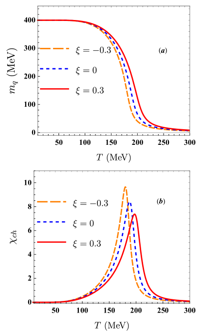
Figure 1: (plot a) The temperature dependences of the constituent quark mass $m_{q}$ at $\mu=0$ MeV for different fixed anisotropy parameters. (plot b) The chiral susceptibility $\chi_{ch}$ at $\mu=0$ MeV for different fixed anisotropy parameters. The broad dashed lines, dashed lines and solid lines represent to the results for $\xi=-0.3$, $\xi=0$ and 0.3, respectively.

The relaxation times of (anti)quarks are microscopically determined by the thermal-averaged elastic scattering cross-section and the particle density. For light quarks, the relaxation time in the RTA can be written as Zhuang:1995uf

$$\tau_{l}^{-1}(T,\mu) = n_{\bar{q}}[\bar{\sigma}_{u\bar{u}\rightarrow u\bar{u}}+\bar{\sigma}_{u\bar{u}\rightarrow d\bar{d}}+\bar{\sigma}_{u\bar{d}\rightarrow u\bar{d}}]$$ (57)

$$n_{q}[\bar{\sigma}_{ud\rightarrow ud}+\bar{\sigma}_{uu\rightarrow uu}],$$

where the number density of (anti-)quarks in weakly aniosotropic medium is given as $n_{q(\bar{q})}=d_{l}\int\frac{d^{3}p}{(2\pi)^{3}}f^{an}_{q(\bar{q})}$ with $d_{l}=d_{\bar{l}}=2N_{c}$ denoting the degeneracy factor. The momenta of the colliding particles for the elastic scattering process $a(\mathbf{p}_{1})+b(\mathbf{p}_{2})\rightarrow c(\mathbf{p}_{3})+d(\mathbf{p}_{4})$ obey the relation $\mathbf{p}_{1}+\mathbf{p}_{2}=\mathbf{p}_{3}+\mathbf{p}_{4}=\mathbf{0}$, and we use the notation $|\mathbf{p}_{1}|=|\mathbf{p}_{2}|=p$ for convenience. In the center-of-mass (c.m.) frame, the mandelstam variables $s,~{}t,~{}u$ are defined as

$$s = 4m_{q}^{2}+4p^{2},t=-2p^{2}(1-\cos\theta_{p}),$$

$$u = -2p^{2}(1+\cos\theta_{p}),$$ (58)

where $\theta_{p}$ is the scattering angle in the c.m. frame. The mandelstam variables hold the relation $u+s+t=4m_{q}^{2}$. $\bar{\sigma}_{ab\rightarrow cd}$ denotes energy-averaged elastic scattering cross-section in the weakly anisotropic system, which can be written as

$$\bar{\sigma}_{ab\rightarrow cd} = \int_{s_{0}}^{\infty}ds\int_{t_{min}}^{t_{max}}dt\frac{d\bar{\sigma}_{ab\rightarrow cd}}{dt}\sin^{2}\theta_{p}\int_{-1}^{1}dx_{3}$$ (59)

$$\times(1-f_{c}^{an}(p_{cm},\mu,x_{3}))\int_{-1}^{1}dx_{4}$$

$$\times(1-f_{d}^{an}(p_{cm},\mu,x_{4}))\mathcal{L}(s,\mu,x_{1},x_{2}),$$

with $(1-f_{c,d}^{an})$ denoting the Pauli-blocking factor for the fermions due to the fact that some of the final states are already occupied by other identical (anti-)quarks. $\frac{d\bar{\sigma}}{dt}=\frac{1}{16\pi s(s-4m_{q}^{2})}|\bar{M}|^{2}$ is differential scattering cross-section. $|\bar{M}|^{2}$ denotes the matrix element squared of a specific scattering process. The formulae of matrix elements squared for various scattering processes are presented in the Appendix. The integration limits of $t$ are $t_{max}=0$ and $t_{min}=-4p_{cm}^{2}=-(s-4m_{q}^{2})$ with $p_{cm}=\sqrt{s-4m_{q}^{2}}/2$ denoting the momentum in the c.m. frame. The kinematic boundary of $s$ reads $s_{0}=4m_{q}^{2}$. The scattering weighting factor $\sin^{2}\theta_{p}=\frac{-4t(s+t-4m_{q}^{2})}{(s-4m_{q}^{2})^{2}}$ is introduced to exclude the scattering processes with the small initial angle because the large angle scattering is dominated in momentum transport process Danielewicz:1984ww . In the c.m. frame, the leading-order anisotropic distribution function can be rewritten as

$$f^{an} (p_{cm},\mu,x)=f^{0}(p_{cm},\mu)$$ (60)

$$-\frac{p_{cm}^{2}\xi x^{2}}{2E_{cm}T}f^{0}(p_{cm},\mu)(1-f^{0}(p_{cm},\mu)),$$

where $E_{cm}=\frac{s-m_{q}^{2}+m_{q}^{2}}{2\sqrt{s}}=\sqrt{s}/2$. In Eq. (59), $\mathcal{L}$ denotes the probability of finding a quark-(anti)quark pair with the center of mass energy $\sqrt{s}$ in the anisotropic medium, which is given as

$$\mathcal{L}=C\sqrt{s(s-4m_{q}^{2})}f_{a}^{an}(p_{cm},\mu,x_{1})f_{b}^{an}(p_{cm},\mu,x_{2})v_{rel}(s),$$ (61)

where $v_{rel}(s)=\sqrt{\frac{s-4m_{q}^{2}}{s}}$ is the relative velocity between two incoming particles in the c.m. frame; $C$ is the normalization constant, and is determined from the requirement that $\int_{s_{0}}^{\infty}ds\int_{-1}^{1}dx_{1}\int_{-1}^{1}dx_{2}\mathcal{L}=1$ with abbreviations $x_{1}=\cos\theta_{1}$ and $x_{2}=\cos\theta_{2}$, $\theta_{i}$ is the angle between $\mathbf{p}_{i}$ and $\mathbf{n}$ and $x_{1}\equiv-x_{3}$, $x_{2}\equiv-x_{4}$. Applying the above formula of relaxation time to Eqs. (44), (V.2), (55), we can calculate the transport coefficients in the QCD medium and study their sensitivity to the momentum anisotropy.

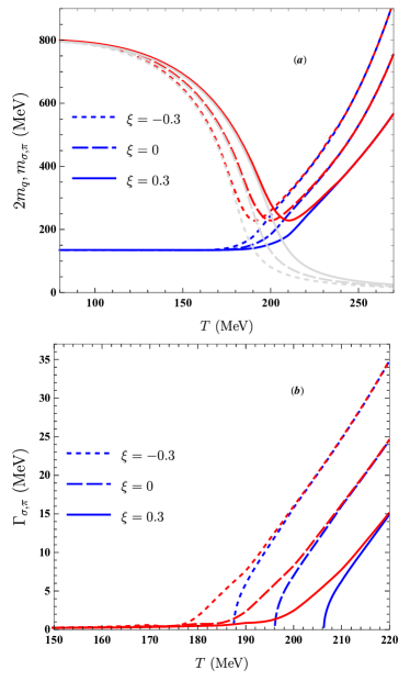
Figure 2: (plot a) The double mass of constituent quarks $2m_{q}$ (gray lines), $\pi$ meson mass (blue lines) and $\sigma$ meson mass (red lines) as a function with temperature at $\mu=0$ GeV for different anisotropy parameter $\xi$. (plot b) The temperature dependences of both $\pi$ (blue lines) and $\sigma$ (red lines) meson decay widths for different $\xi$. The broad dashed lines, dashed lines and solid lines represent to the results for $\xi=-0.3$, $\xi=0$, and 0.3, respectively. The respective Mott temperatures are approximately 187 $\mathrm{MeV}$, 196 $\mathrm{MeV}$, 206 $\mathrm{MeV}$ for $\xi=-0.3,~{}0,~{}0.3$.

VII Results and discussion

Throughout this work, the following parameter set is used: $m_{0}=m_{0,u}=m_{0,d}=5.6~{}\mathrm{MeV}$, $G\Lambda^{2}=2.44$ and $\Lambda=587.9~{}\mathrm{MeV}$. These values are taken from Ref. Buballa:2003qv , where these parameters are determined by fitting quantities in the vacuum ($T=\mu=0$ MeV). At $T=0$, the chiral symmetry is spontaneously broken and one obtain the current pion mass $m_{0,\pi}=135$ MeV, the pion decay constant $f_{\pi}=92.4$ MeV, the quark condensate $-\langle\psi\psi\rangle^{1/3}=241$ MeV.

In the NJL model, the constituent quark mass is a good indicator and an order parameter for analyzing the dynamical feature of chiral symmetry. In the asymptotic expansion-driven momentum anisotropic system, the anisotropy parameter $\xi$ is always positive due to the rapid expansion along the beam direction. Whereas, in the strong magnetic field-driven momentum anisotropic system, $\xi$ is always negative due to the reduction of transverse momentum in Landau quantization. Since we restrict the analysis to only weakly anisotropic medium, the anisotropy parameters we work here are artificially taken as $\xi=-0.3,~{}0.0,~{}0.3$, to phenomenologically investigate the effect of $\xi$ on various quantities. In Fig. 1 (a), we show the thermal behavior of light constituent quark mass $m_{q}$ for vanishing quark chemical potential at different $\xi$. For low temperature, $m_{q}$ remains approximately constant ($m_{q}\approx$ 400 MeV), then with increasing temperature $m_{q}$ continuously drops to near zero. The transition to small mass occurs at higher temperature for higher value of $\xi$. These phenomena imply that at zero chemical potential the restoration of the chiral symmetry (the chiral symmetry is not strictly restored) because the current quark mass is nonzero) in an (an-)isotropic quark matter takes place as crossover phase transition, and an increase in $\xi$ can lead a catalysis of chiral symmetry breaking.

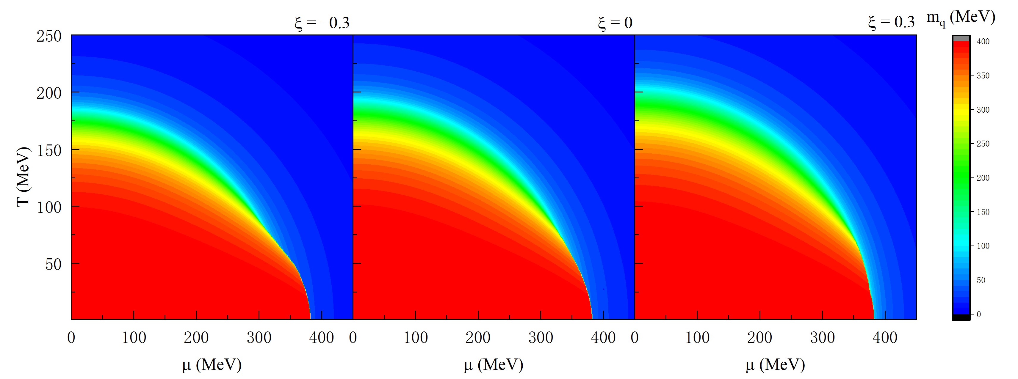
Figure 3: The 3-dimensional plot of constituent quark mass $m_{q}$ with respect to temperature and quark chemical potential for different anisotropy parameters ($\xi=-0.3,~{}0,~{}0.3$).

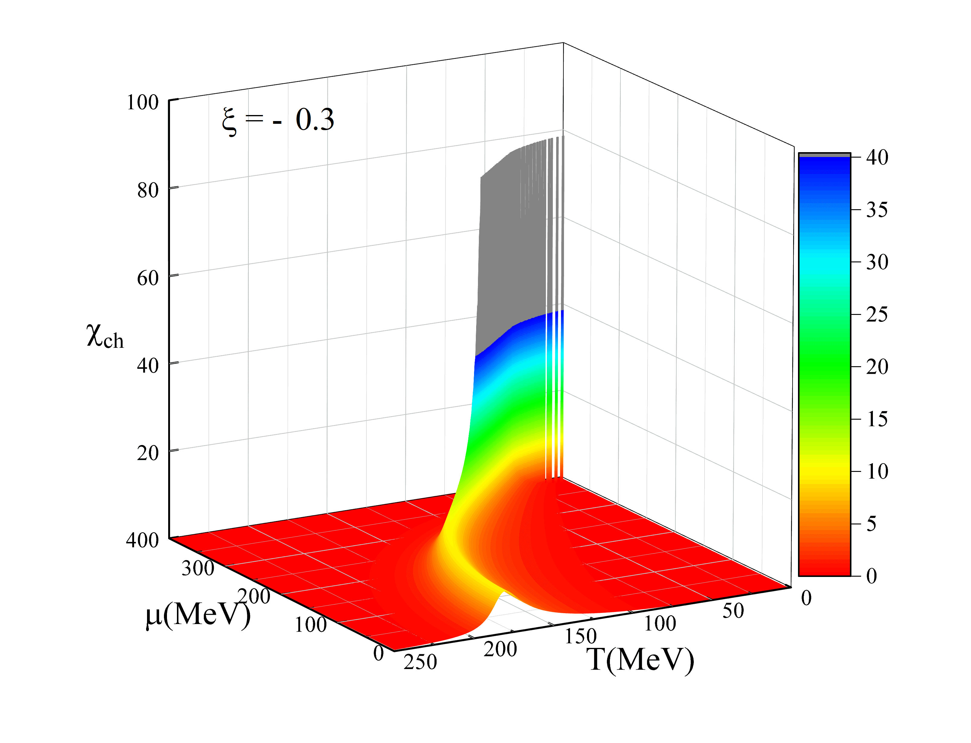
Figure 4: The 3-dimensional plot of chiral susceptibility $\chi_{ch}$ for $\xi=-0.3$ in the entire $\mu$ and $T$ ranges of interest. The gray area means $\chi_{ch}$ is divergent. (The values remain finite due to numerical problems (differential quotient). The peak height at high $\mu$ is two orders of magnitude higher than in small $\mu$ cases and can be considered ”divergent”.)

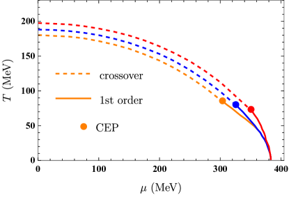
Figure 5: The chiral phase diagram for different anisotropy parameters in the NJL model. The solid lines denote the first-order phase transition curves, the dashed lines denote the crossover transition curves, and the solid dots represent the CEPs. We observe that the CEP is shifted towards larger values of the quark chemical potential but smaller values of the temperature for higher anisotropy parameters.

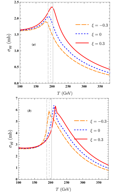
Figure 6: (plot $a$) The cross-section of total quark-quark scattering processes $\bar{\sigma}_{qq}$ as a function of temperature at $\mu=0$ MeV for different anisotropy parameters. (plot $b$) The cross-section of total quark-antiquark scattering processes $\bar{\sigma}_{q\bar{q}}$ as a function of temperature at $\mu=0$ MeV for different anisotropy parameters, i.e., $\xi=-0.3$ (orange broad dashed line), $\xi=0$ (blue dashed line),  $\xi=0.3$ (red solid line). The gray vertical lines (from left to right) represent the critical temperatures $T_{c}=$ 180 MeV, 188 MeV, 197 MeV for $\xi=-0.3,~{}0,~{}0.3$.

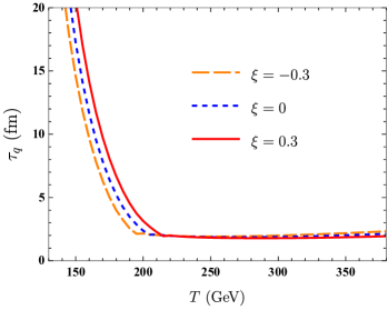
Figure 7: The relaxation time of quark at $\mu=0$ MeV as a function of temperature for different anisotropy parameters, i.e., $\xi=-0.3$ (orange broad dashed line), $\xi=0$ (blue dashed line),  $\xi=0.3$ (red solid line).

In this work, the chiral critical temperature, $T_{c}$, is determined by the peak location of the associated chiral susceptibility $\chi_{ch}$, which is defined as $\chi_{ch}=\big{|}\frac{dm_{q}}{dT}\big{|}$. We stress that the criterion of obtaining the chiral critical temperature is different in different papers, and there are some shortcomings in the NJL model, such as parameter ambiguity, nonrenormalization and the absence of gluonic dynamics, so the value of $T_{c}$ in present work is not expected to quantitatively describe the lattice QCD result. Anyway, these cannot affect our present qualitative results. The temperature dependence of chiral susceptibility $\chi_{ch}$ for different $\xi$ at $\mu=0$ MeV is plotted in Fig. 1 (b). We observe that $T_{c}$ exhibits a significant $\xi$ dependence. As $\xi$ increases, $T_{c}$ shifts toward higher temperatures and the height of peak decreases. The locations of $T_{c}$ for $\xi=-0.3,~{}0,~{}0.3$ are $\sim$ 180 MeV, 188 MeV, 197 MeV, which means a change of about 10$\%$ in temperature. Actually, the in-medium meson masses also can be regarded as a signature of chiral phase transition. In Fig. 1(a), we display the variation of $\pi$ and $\sigma$ meson masses with temperature for different $\xi$ at $\mu=0$ MeV. As can be seen that the $\pi$ mass remains approximately constant up to a particular temperature whereas the $\sigma$ mass first decreases and then increases. As temperature increases further, difference between $\pi$ mass and $\sigma$ mass also decreases and finally vanishes, at this time, $\sigma$ and $\pi$ mesons are degenerate and become unphysicals degrees of freedom, which indicates the restoration of chiral symmetry. And before $\pi$ and $\sigma$ meson masses emerge, $\pi$ mass decreases as $\xi$ increase beyond $T_{c}$, whereas $\sigma$ mass first increases and then decreases with the increase of $\xi$. This qualitative behavior of meson masses with $\xi$ also is observed in our previous report Zhang:2020zrv based on the quark-meson model. Our result also slightly differs from the finite size study of the NJL model Deb:2020qmx , which shows that below the critical temperature, $\pi$ mass enhances as the system size decreases, while $\sigma$ mass first remains unchanged then increases. Furthermore, we see that at a certain temperature, two times constituent quark mass ($2m_{q}$) is equal to $\pi$ mass, the pion meson is no longer a bound state but only a $q\bar{q}$ resonance and obtains a finite decay width. Accordingly, the Mott transition temperature by the definition $m_{\pi}(T_{Mott})=2m_{q}(T_{Mott})$ can be obtained. The Mott temperatures for $\xi=-0.3,~{}0$ and 0.3 turn out to be $\sim$ 187 MeV, 196 MeV and 206 $\mathrm{MeV}$, respectively, which is slightly higher than the corresponding $T_{c}$. In the vicinity of the Mott temperature, $\sigma$ meson features its minimal mass. In Fig. 2 (b), we illustrate the variation of the decay widths of both $\sigma$ and $\pi$ mesons with temperature for different $\xi$. As can be seen, the decay width of $\sigma$ meson, $\Gamma_{\sigma}$, exists in the entire temperature range whereas the decay width of $\pi$ meson, $\Gamma_{\pi}$, starts after the Mott temperature. At high temperature, the merging behaviors of decay widths for different mesons are also observed. And with the increase of $\xi$, the decay widths of mesons have a reduction.

We continue the analysis in finite quark chemical potential case to investigate the effect of momentum anisotropy on the phase boundary and the CEP position. First, we display the temperature- and quark chemical potential-dependence of constituent quark mass $m_{q}$ for different anisotropy parameters, as shown in Fig. 3. We can see that at small $\mu$, $m_{q}$ continuously decreases with increasing $T$, whereas $m_{q}$ has a significant discontinuity or a sharp drop along $T$-axis at sufficiently high $\mu$, which is usually considered as the appearance of the first-order phase transition. To visualize the phase diagram we use the significant divergency of $\chi_{ch}$ at sufficiently high chemical potential as the criterion for a first-order phase transition, as shown in Fig. 4. With the decrease of $\mu$, the first-order phase transition terminates at a critical endpoint (CEP), where the phase transition is expected to be of second order. As $\mu$ decreases further, the maximum of the chiral susceptibility ($\chi_{ch}$) as the crossover criterion. The full chiral boundary lines in the ($\mu$-$T$) plane for three different values of $\xi$ are displayed in Fig. 5. We observe that as the increase of $\xi$, the phase boundary shifts toward higher quark chemical potentials and higher temperatures. We also can see the CEP position is sensitive to the variation of $\xi$. As $\xi$ increases, the location of CEP shifts to higher $\mu$ and smaller $T$. The CEP location ($T_{CEP},~{}\mu_{CEP}$) in this work are separately presented at (298.70 $\mathrm{MeV}$, 88.2 $\mathrm{MeV}$), (321.8 $\mathrm{MeV}$, 82.4 $\mathrm{MeV}$), (348.4 $\mathrm{MeV}$, 74.2 $\mathrm{MeV}$) for $\xi=-0.3,~{}0,~{}0.3$. The the position of CEP for $\xi=0$ in this work is almost consistent with the existing result Chaudhuri:2019lbw in the same parameter fit. The value of $\mu_{CEP}$ ($T_{CEP}$) from $\xi=-0.3$ to $\xi=0.3$ increases (decreases) by approximately 16$\%$ (17$\%$), in other words, the influence degree of momentum anisotropy on temperature of CEP is almost the same as that on the quark chemical potential of CEP. This is different to the result of Ref. Zhang:2020zrv , which has shown that in the quark meson model the impact of momentum anisotropy on the quark chemical potential of the CEP is significantly dominant than that on the associated temperature. In addition, in the study of finite volume effect, the result of Ref. Bhattacharyya:2012rp has indicated that in the PNJL model the finite volume affects the CEP shift along the temperature more strongly than along the quark chemical potential shift. And when the system size is reduced to 2 fm, the CEP in the PNJL model vanishes and the whole chiral phase boundary becomes a crossover curve. Based on this result, there also exists a possibility that if $\xi$ further increases, the CEP may disappear from the phase diagram.

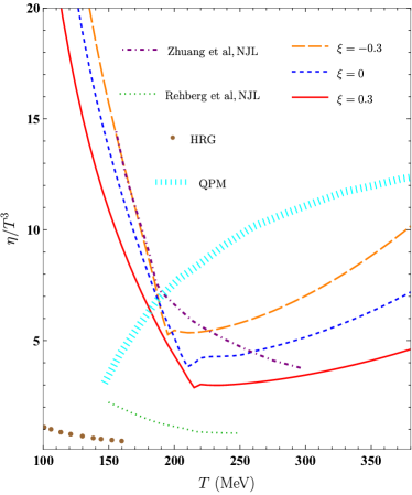
Figure 8: The temperature dependence of scaled shear viscosity $\eta/T^{3}$ in quark matter at vanishing chemical potential for different anisotropy parameters i.e., $\xi=$ $-0.3$ (orange broad dashed line), $\xi=0$ (blue dashed line), and $\xi=0.3$ (red solid line). The thick cyan dotted line represents the result in the $N_{f}=3$ quasiparticle model (QPM) shear-quasi2 , which is an effective model for the description of non-perturbative QCD. The purple dotdashed line shows the result obtained in the $N_{f}=2$ NJL model by Zhuang $et~{}al$ Zhuang:1995uf . The brown dots show the result from hadron resonance gas (HRG) model shear and electrical . The green dots correspond to the result of Rehberg $et~{}al$ in the $N_{f}=3$ NJL model Rehberg:1996vd using the averaged transition rate method for the estimation of relaxation time.

Figure 9: The temperature dependence of scaled electrical conductivity $\sigma_{el}/T$ in quark matter at vanishing chemical potential for different anisotropy parameters i.e., $\xi=$ $-0.3$ (orange broad dashed line), $\xi=0$ (blue dashed line), and $\xi=0.3$ (red solid line). The green dotted line shows the result of Marty $et~{}al$ in $N_{f}=3$ NJL model Marty:2013ita . The thick gray dotdashed line represents the result from the pQCD-based microscopic Boltzmann Approach to Multi-Parton Scatterings (BAMPS) transport model Greif:2014oia with running coupling constant. The brown stars present the result in the Parton-Hadron-String Dynamics (PHSD) transport approach Steinert:2013fza . The cyan dotdashed line shows the result within excluded volume hadron resonance gas (EVHRG) model with the RTA electrical-EVHRG . The darkyellow dots are the lattice date obtained from Ref. Amato:2013naa . The red open circles are the calculation for hadronic gas in the transport approach- Simulating Many Accelerated Strongly-interacting Hadrons (SMASH) Hammelmann:2018ath based on Green-Kubo formalism.

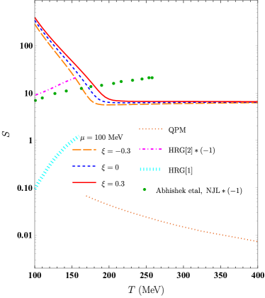
Figure 10: The temperature dependence of Seebeck coefficient in quark matter at $\mu=100$ MeV for different anisotropy parameters i.e., $\xi=$ $-0.3$ (orange broad dashed line), $\xi=0$ (blue dashed line), and $\xi=0.3$ (red solid line). The brown dotted line corresponds to the result for the QGP in the quasiparticle model Dey:2020sbm at $\mu_{q}=50$ MeV. The cyan thick-dotted line represents the result in hadron resonance gas model for $\mu_{B}=0.1$ GeV Bhatt:2018ncr , The mauve dotdashed line and green dots, respectively, represent the results in HRG model for $\mu_{B}=50$ MeV Das:2020beh and the $N_{f}=2$ NJL model for $\mu=100$ MeV Abhishek:2020wjm , where the gradient of quark chemical potential apart from a spatial gradient in temperature also is included.

To better understand the qualitative behavior of transport coefficients, we first discuss the results of the scattering cross-sections and the relaxation time. In Fig 6, we display the cross-section of total quark-quark scattering processes $\bar{\sigma}_{qq}=\bar{\sigma}_{uu\rightarrow uu}+\bar{\sigma}_{ud\rightarrow ud}$ (plot $a$) and the cross-section of total quark-antiquark processes $\bar{\sigma}_{q\bar{q}}=\bar{\sigma}_{u\bar{u}\rightarrow u\bar{u}}+\bar{\sigma}_{u\bar{d}\rightarrow u\bar{d}}+\bar{\sigma}_{u\bar{u}\rightarrow d\bar{d}}$ (plot $b$) as functions of temperature at different anisotropy parameters for vanishing quark chemical potential. As can be seen, $\bar{\sigma}_{qq}$ and $\bar{\sigma}_{q\bar{q}}$ have similar peak features in entire temperature region of interest. More exact, the scattering cross-sections first increase, reaches a peak, and decreases with increasing temperature afterwards. And the magnitude of $\bar{\sigma}_{q\bar{q}}$ is higher than that of $\bar{\sigma}_{qq}$. This is mainly due to that the $s$ channel allows for a resonance of the exchanged meson with the incoming quarks, which leads to a large peak in the cross-section Soloveva:2020hpr . We can also see that the scattering cross-sections in the weakly anisotropic medium keep the same behaviors as those in the isotropic medium. As $\xi$ increases, $\bar{\sigma}_{qq}$ increases in the entire temperature domain of considered, whereas $\bar{\sigma}_{q\bar{q}}$ first decreases as $\xi$ increases and then increases as $\xi$ increases. With an increase in $\xi$, the maximum of the scattering cross-section shifts toward higher temperatures. The location of maximum for $\bar{\sigma}_{qq}$ at different $\xi$ is nearly in agreement with respective $T_{c}$. While the peak positions of $\bar{\sigma}_{q\bar{q}}$ respectively locate at $\sim 1.07~{}T^{-0.3}_{c}$, $1.07~{}T^{0}_{c}$, $1.10~{}T^{0.3}_{c}$ for $\xi=-0.3,~{}0,~{}0.3$ with $T^{\xi}_{c}$ denoting the chiral critical temperature for a fixed $\xi$.

The dependence of total quark relaxation time $\tau_{q}$ on temperature for vanishing quark chemical potential at different $\xi$ is displayed in Fig. 7. As can be seen, $\tau_{q}$ first decreases sharply with increasing temperature, after an inflection point ($viz$, the peak position of $\bar{\sigma}_{q\bar{q}}$), $\tau_{q}$ is modestly changing with temperature. And the increase of $\tau_{q}$ with $\xi$ is significant at low temperature whereas at high temperature the reduction of $\tau_{q}$ with $\xi$ is imperceptible. This is the result of the competition between the quark number density and the total scattering cross section in Eq. (57). At small temperature, the $\xi$ dependence of $\tau_{q}$ is mainly determined by the inverse quark number density whereas at high temperature it is primarily governed by the inverse total cross-section even though this effect is largely cancelled out by the inverse quark density effect.

Next, we are going to discuss the results regarding various transport coefficients. In Fig. 8, the temperature dependence of scaled shear viscosity $\eta/T^{3}$ in quark matter for different momentum anisotropy parameters at a vanishing chemical potential is displayed. We observe that with increasing temperature, $\eta/T^{3}$ first decreases, reaches a minimum around the critical temperature, and increases afterwards. The temperature position of minimum for $\eta/T^{3}$ is consistent with the temperature of peak for $\bar{\sigma}_{q\bar{q}}$. This dip structure of $\eta/T^{3}$ can mainly depend on the result of a competition between quark distribution function $f^{0}_{q}$ and quark relaxation time $\tau_{q}$ in the integrand of Eq. (44). The increasing feature of $\eta/T^{3}$ in low temperature domain is governed by $\tau_{q}$, while in high temperature domain the increasing behavior of $f^{0}_{q}$ overwhelms the decreasing behavior of $\tau_{q}$, leading $\eta/T^{3}$ become an increasing function of temperature. Furthermore, we observe that as an increase in $\xi$, $\eta/T^{3}$ has an overall enhancement and the minimum of $\eta/T^{3}$ shifts to higher temperatures. The location of the minimum for $\eta/T^{3}$ at different $\xi$ is consistent with the peak position of $\bar{\sigma}_{q\bar{q}}$. And we observe that $\eta/T^{3}$ decreases as $\xi$ increases in entire temperature region. we also compare our result for $\xi=0$ with the results reported in other previous literature. The calculation of $\eta/T^{3}$ in hadron resonance gas (HRG) model shear and electrical (brown dots) using the RTA is a decreasing function with temperature, which is qualitatively similar to ours below the critical temperature. The quantitative difference between HRG model result and ours can be attributed to the uses of various degrees of freedom and the difference of scattering cross-sections. The result of Zhuang $et~{}al$ Zhuang:1995uf in the $N_{f}=2$ NJL model (purple dotdashed line) is of the same order of magnitude as ours, while at high temperature their result still remains a decreasing feature because an ultraviolet cutoff is used in all momentum integral whether temperature is finite or zero. The result estimated in the quasiparticle (QPM) shear-quasi2 is a logarithmically increasing function of temperature beyond the critical temperature, and is quantitively larger than ours beyond critical temperature due to the differences in both the effective mass of quark and the relaxation time. The result of Rehberg $et~{}al$ Rehberg:1996vd for the $N_{f}=3$ NJL model in the temperature regime close to the critical temperature is smaller than ours, and the obvious dip structure is not observed because the momentum cutoff is also used at finite temperature.

In Fig. 9, we plot the thermal behavior of scaled electrical conductivity $\sigma_{el}/T$ at $\mu=0$ MeV for different $\xi$. Similar to the temperature dependence of $\eta/T^{3}$, $\sigma_{el}/T$ also exhibits a dip structure in the entire temperature region of interest. We also present the comparison with other previous results. The result obtained from the PHSD approach Steinert:2013fza (brown stars), where the plasma evolution is solved by a Kadanoff-Baym type equation, also has a valley structure, eventhough the location of the minimum is different with ours. We also observe that in the temperature region dominated by hadronic phase, the thermal behavior of $\sigma_{el}/T$ using the microscopic simulation code SMASH Hammelmann:2018ath (pink open circles) is similar to ours. Furthermore, our result is much larger than the lattice QCD data (darkyellow dots) taken from Ref. Amato:2013naa due to the uncertainity in the parameter set and the uninclusion of gluonic dynamics. The result within exclude volume hadron resonance gas (EVHRG) modelelectrical-EVHRG (cyan dotdashed line) and the result obtained from partonic cascade BAMPS Greif:2014oia (gray thick dotdashed line) are in the both qualitative and quantitive similar to our calculations below the critical temperature and beyond the critical temperature, respectively. Our shape is similar to the result of Marty $et~{}al$ obtained within the $N_{f}=3$ NJL model Marty:2013ita (green dotted line), the numerical discrepancy mainly comes from the differences in both the parameter set and the normalization of the scattering cross-section. In addition, $\sigma_{el}/T$ shows a different $\xi$ dependence than $\eta/T^{3}$. More exact, $\sigma_{el}/T$ first increases as $\xi$ whereas, as $T$ increases further, the values $\sigma_{el}/T$ for different $\xi$ gradually approach and eventually overlap, which is different to the result in Ref. Srivastava:2015via . In Ref. Srivastava:2015via , $\sigma_{el}/T$ of the QGP is a monotonic increasing function of $\xi$ because the effect of momentum anisotropy is not incorporated in the calculation of the relaxation time and the effective mass of quasiparticles, the $\xi$ dependence of $\sigma_{el}/T$ is only determined by the anisotropic distribution function. We also observe that with the increase of $\xi$, the minimum of $\sigma_{el}/T$ shifts to higher temperatures, which is similar to $\eta/T^{3}$, however, the height of the minimum increase, which is opposite to $\eta/T^{3}$.

Finally, we study Seebeck coefficient $S$ in quark-antiquark matter. Due to the sensitivity of $S$ to charge type of particle species, at a vanishing chemical potential, quark number density $n_{q}$ is equal to antiquark number density $n_{\bar{q}}$, the contribution of quarks to $S$ is exactly compensated with the counterpart of antiquarks. Thus, a finite quark chemical potential is required to obtain a non-zero thermoelectric current in the medium. In Fig. 10, we plot the variation of $S$ with respect to temperature for different $\xi$ at $\mu=100$ MeV. The comparison with other previous calculations, which are all performed in the kinetic theory under the RTA, also is presented. We remind the reader that at a finite $\mu$, $n_{q}$ is larger than $n_{\bar{q}}$, the contribution of quarks to total $S$ in magnitude is always prominent. As shown in Fig. 10, the sign of $S$ in our investigation is positive, which indicates that the dominant carriers of converting heat gradient to the electric field is positively charged quarks, i.e., $up$ quarks. Actually, the positive or negative of $S$ is mainly determined by the factor $(E_{q}-\mu_{q})$ in the integrand of Eq. (55). In Ref. Dey:2020sbm , Seebeck coefficient studied in the QPM (brown dotted line) at $\mu=50$ MeV also exhibits a decreasing feature with increasing temperature. The result of Abhishek $et~{}al$ Abhishek:2020wjm at $\mu=100~{}$MeV in the $N_{f}=2$ NJL model (the green dots) is much different with ours. In Ref. Abhishek:2020wjm , $S$ is negative and its absolute value exhibits an increasing function with temperature. The reasons behind this quantitative and qualitative discrepancy are twofold: (1) the relaxation time in Ref. Abhishek:2020wjm is estimated by using the averaged transition rate $\bar{w}_{ij}$ while our relaxation time is obtained from the thermally averaged cross-section of elastic scattering (the detailed comparison of two methods can be found in Ref. Soloveva:2020hpr ); (2) in Ref. Abhishek:2020wjm , the spatial gradient of chemical potential also is included apart from the temperature gradient, accordingly the sign of $S$ is mainly determined by a factor $(E_{q}-\omega/n_{q})$ with $\omega$ denoting the enthalpy density in the associated formalism. Due to the single-particle energy $E_{q}$ remains smaller than $(\omega/n_{q})$, $S$ in Ref. Abhishek:2020wjm is negative. We also see that with increasing temperature, $S$ sharply decreases below $T_{c}$, whereas the decreasing feature of $S$ is unconspicuous above $T_{c}$. And the value of $S$ at low $T$ is much larger than that at high $T$. This also is different to the result in Ref. Abhishek:2020wjm , where the absolute value of $S$ in quark matter increases with increasing temperature because of the increasing behaviors of both the factor $|-\omega/n_{q}|$ and the equilibrium distribution function. In addition, Seebeck coefficient in HRG model Das:2020beh ; Bhatt:2018ncr is also positive (negative) without (with) the spatial gradient of chemical potential (cyan thick dotted line and mauve dotdashed line). Nevertheless, the absolute value of $S$ in hadronic matter is still an increasing function of temperature regardless of the spatial gradient of $\mu$. We also see that as $\xi$ increases, $S$ has a quantitative enhancement, which is mainly due to a significant rise in the thermoelectric conductivity $\alpha$, eventhough $1/\sigma_{el}$ has a cancellation effect on the increase of $S$. At sufficiently high temperature, the rise in $1/\sigma_{el}$ can almost compensate with the reduce of $\alpha$, as a result, $S$ varies unsignificantly with $\xi$ of interest, compared to the value of $S$ itself.

VIII Summary

We phenomenologically investigated the impact of weak momentum-space anisotropy on the chiral phase structure, mesonic properties, and transport properties in the 2-flavor NJL model. The momentum anisotropy, which is induced by initial preferential expansion of created fireball in heavy-ion collisions along the beam direction, can be incorporated in the calculation through the parameterization of anisotropic distribution function. Our result has shown that the chiral phase transition is a smooth crossover for vanishing quark chemical potential, independent of anisotropy parameter $\xi$, and an increase in $\xi$ even can hinder the restoration of the chiral symmetry. We found the CEP highly sensitive to the change in $\xi$. With the increase of $\xi$, the CEP shifts to higher $\mu$ and smaller $T$, and the momentum anisotropy affects the CEP temperature to almost the same degree as it affects the CEP chemical potential. Before the merge of $\pi$ and $\sigma$ meson masses, the $\xi$ dependence of $\pi$ meson mass is opposite to that of $\sigma$ meson mass.

We also studied the thermal behavior of various transport coefficient, such as scaled shear viscosity $\eta/T^{3}$, scaled electrical conductivity $\sigma_{el}/T$ and Seebeck coefficient $S$ at different $\xi$. The associated $\xi$-dependent expressions are derived by solving the relativistic Boltzmann-Vlasov transport equation in the relaxation time approximation, and the momentum anisotropy effect also is embedded in the estimate of relaxation time. We found $\eta/T^{3}$ and $\sigma_{el/T}$ have a dip structure around the critical temperature. Within the consideration of momentum anisotropy, $\eta/T^{3}$ decreases as $\xi$ increases and the minimum shifts to higher temperatures. As the increase of $\xi$, $\sigma_{el}/T$ significantly increases for low temperature whereas the sensitivity of $\sigma_{el}/T$ to $\xi$ for high temperature is greatly reduced, which is different from the behavior of $\eta/T^{3}$ with $\xi$. We also found the sign of $S$ at $\mu=100$ MeV in present work is positive, indicating the dominant carriers for converting the thermal gradient to the electric field are $up$ quarks. And with increasing temperature, $S$ first decreases sharply then almost flattens out. At low temperature, $S$ significantly increases with an increase of $\xi$, whereas at high temperature the rise is marginal compared to the value of $S$ itself.

We note it is of strong interest to include the Polyakov-loop potential in the present model to study both chiral and confining dynamics in an anisotropic quark matter. And a more realistic ellipsoidal momentum anisotropy characterized by two independent anisotropy parameters can be applied to gain a deeper understanding of the QGP properties. In present work, there is no any proper time dependence has been given to the anisotropy parameter. However, in the realistic case, $\xi$ varies with the proper time starting from the initial proper time up to a time when the system becomes isotropic. Thus, we also can introduce a proper time dependence to the anisotropy parameterMartinez:2008di to better explore the effect of time-dependent momentum anisotropy on chiral phase transition. In addition, the investigation of the thermoelectric coefficients specially the magneto-Seebeck coefficient and Nernst coefficient in magnetized quark matter based the PNJL model would be an attractive direction, and we may work on it in the near future.

Appendix

In the $N_{f}=2$ NJL model, there are 12 different elastic scattering processes:

$$u\bar{u}\rightarrow u\bar{u},~{}u\bar{d}\rightarrow u\bar{d},~{}u\bar{u}\rightarrow d\bar{d},$$

$$uu\rightarrow uu,~{}ud\rightarrow ud,~{}\bar{u}\bar{u}\rightarrow\bar{u}\bar{u},$$

$$\bar{u}\bar{d}\rightarrow\bar{u}\bar{d},~{}d\bar{d}\rightarrow d\bar{d},~{}d\bar{d}\rightarrow u\bar{u},$$

$$d\bar{u}\rightarrow d\bar{u},~{}dd\rightarrow dd,~{}\bar{d}\bar{d}\rightarrow\bar{d}\bar{d}.$$ (62)

The explicit expressions of the matrix elements squared for $u\bar{u}\rightarrow u\bar{u}$, $u\bar{d}\rightarrow u\bar{d}$ and $ud\to ud$ processes via exchange of scalar and/or pseudoscalar mesons to $1/N_{c}$ order are given as

$$|\bar{M}_{u\bar{u}\rightarrow u\bar{u}}|^{2}(s,t) = s^{2}|D^{\pi}_{s}|^{2}+t^{2}|D^{\pi}_{t}|^{2}+(s-4m^{2})^{2}|D^{\sigma}_{s}|^{2}+(t-4m^{2})^{2}|D^{\sigma}_{t}|^{2}+\frac{1}{N_{c}}Re\bigg{[}stD^{\pi^{*}}_{s}D^{\pi}_{t}+s(4m^{2}-t)D^{\pi^{*}}_{s}D^{\sigma}_{t}$$ (63)

$$+t(4m^{2}-s)D^{\pi}_{t}D^{\sigma^{*}}_{s}+(st+4m^{2}(s+t)-16m^{4})D^{\sigma}_{t}D^{\sigma^{*}}_{s}\bigg{]},$$

$$|\bar{M}_{u\bar{d}\rightarrow u\bar{d}}|^{2}(s,t) = 4s^{2}|D^{\pi}_{s}|^{2}+t^{2}|D^{\pi}_{t}|^{2}+(t-4m^{2})^{2}|D^{\sigma}_{t}|^{2}-\frac{1}{N_{c}}Re\bigg{[}2stD^{\pi^{*}}_{s}D^{\pi}_{t}+2s(4m^{2}-t)D^{\pi^{*}}_{s}D^{\sigma}_{t}\bigg{]},$$ (64)

$$|\bar{M}_{ud\rightarrow ud}|^{2}(t,u) = 4u^{2}|D^{\pi}_{u}|^{2}+t^{2}|D^{\pi}_{t}|^{2}+(t-4m^{2})^{2}|D^{\sigma}_{t}|^{2}-\frac{1}{N_{c}}Re\bigg{[}2utD^{\pi^{*}}_{s}D^{\pi}_{t}+2u(4m^{2}-t)D^{\pi^{*}}_{u}D^{\sigma}_{t}\bigg{]}.$$ (65)

The meson propagators in the above are $\xi$-dependent. Based on above formulae of three scattering processes, the matrix element squared for remaining scattering processes can be obtained through charge conjugation and crossing symmetry Friesen:2013bta ; Zhuang:1995uf .

References

- (1) C. Bernard et al. [MILC Collaboration], Phys. Rev. D 71, 034504 (2005).
- (2) Y. Aoki, Z. Fodor, S. D. Katz and K. K. Szabo, Phys. Lett. B 643, 46 (2006)
- (3) Y. Aoki, G. Endrodi, Z. Fodor, S. D. Katz and K. K. Szabo, Nature 443, 675 (2006).
- (4) S. Borsanyi, G. Endrodi, Z. Fodor, A. Jakovac, S. D. Katz, S. Krieg, C. Ratti and K. K. Szabo, JHEP 1011, 077 (2010).
- (5) S. Borsanyi, Z. Fodor, C. Hoelbling, S. D. Katz, S. Krieg and K. K. Szabo, Phys. Lett. B 730, 99 (2014).
- (6) A. Bazavov et al. [HotQCD Collaboration], Phys. Rev. D 90, 094503 (2014).
- (7) K. Splittorff and J. J. M. Verbaarschot, Phys. Rev. D 75, 116003 (2007).
- (8) A. Barducci, R. Casalbuoni, S. De Curtis, R. Gatto and G. Pettini, Phys. Lett. B 231, 463 (1989).
- (9) M. Asakawa and K. Yazaki, Nucl. Phys. A 504, 668 (1989).
- (10) A. Bazavov et al. [HotQCD Collaboration], Phys. Lett. B 795, 15 (2019).
- (11) R. V. Gavai and S. Gupta, Phys. Rev. D 68, 034506 (2003).
- (12) C. R. Allton, S. Ejiri, S. J. Hands, O. Kaczmarek, F. Karsch, E. Laermann and C. Schmidt, Phys. Rev. D 68, 014507 (2003).
- (13) E. Laermann, F. Meyer and M. P. Lombardo, J. Phys. Conf. Ser. 432, 012016 (2013).
- (14) O. Philipsen and C. Pinke, Phys. Rev. D 93, no. 11, 114507 (2016).
- (15) Z. Fodor and S. D. Katz, Phys. Lett. B 534, 87 (2002)
- (16) K. Fukushima and C. Sasaki, Prog. Part. Nucl. Phys. 72, 99 (2013).
- (17) P. Braun-Munzinger, V. Koch, T. Schäfer and J. Stachel, Phys. Rept. 621, 76 (2016).
- (18) Y. Nambu and G. Jona-Lasinio, Phys. Rev. 124, 246 (1961); 122, 345 (1961).
- (19) U. Vogl and W. Weise, Prog. Part. Nucl. Phys. 27, 91 (1991). R. Alkofer, H. Reinhardt and H. Weigel, Phys. Rep. 265, 139 (1996).
- (20) S. Klevansky, Rev. Mod. Phys. 64, 649 (1992); E. Quack and S. P. Klevansky, Phys. Rev. C 49, 3283-3288 (1994).
- (21) M. Buballa, Phys. Rept. 407, 205 (2005).
- (22) C. Ratti, S. Roessner, M. A. Thaler and W. Weise, Eur. Phys. J. C 49, 213 (2007).
- (23) S. Mukherjee, M. G. Mustafa and R. Ray, Phys. Rev. D 75, 094015 (2007).
- (24) P. Costa, M. C. Ruivo, C. A. de Sousa and H. Hansen, Symmetry 2, 1338 (2010).
- (25) K. Fukushima, Phys. Rev. D 77, 114028 (2008) Erratum: [Phys. Rev. D 78, 039902 (2008)].
- (26) B. J. Schaefer and J. Wambach, Phys. Rev. D 75, 085015 (2007).
- (27) B. J. Schaefer and M. Wagner, Phys. Rev. D 79, 014018 (2009).
- (28) R. A. Tripolt, N. Strodthoff, L. von Smekal and J. Wambach, Phys. Rev. D 89, no. 3, 034010 (2014).
- (29) B. J. Schaefer, J. M. Pawlowski and J. Wambach, Phys. Rev. D 76, 074023 (2007).
- (30) V. Skokov, B. Stokic, B. Friman and K. Redlich, Phys. Rev. C 82, 015206 (2010).
- (31) B. J. Schaefer and M. Wagner, Phys. Rev. D 85, 034027 (2012).
- (32) P. Zhuang, J. Hufner and S. P. Klevansky, Nucl. Phys. A 576, 525 (1994).
- (33) Z. Zhang, C. Shi, X. T. He, X. Luo and H. S. Zong, Phys. Rev. D 102, 114023 (2020).
- (34) Y. Jiang and J. Liao, Phys. Rev. Lett. 117, no. 19, 192302 (2016).
- (35) R. Gatto and M. Ruggieri, Phys. Rev. D 83, 034016 (2011).
- (36) K. Kashiwa, Phys. Rev. D 83, 117901 (2011).
- (37) M. D’Elia, F. Manigrasso, F. Negro and F. Sanfilippo, Phys. Rev. D 98, no. 5, 054509 (2018).
- (38) J. O. Andersen, W. R. Naylor and A. Tranberg, JHEP 1404, 187 (2014).
- (39) M. R. B. Ferreira, QCD phase diagram under an external magnetic field, 2015.
- (40) G. S. Bali, F. Bruckmann, G. Endrodi, Z. Fodor, S. D. Katz, S. Krieg, A. Schafer and K. K. Szabo, JHEP 1202, 044 (2012).
- (41) S. S. Wan, D. Li, B. Zhang and M. Ruggieri, arXiv:2012.05734 [hep-ph].
- (42) Y. P. Zhao, R. R. Zhang, H. Zhang and H. S. Zong, Chin. Phys. C 43, no. 6, 063101 (2019).
- (43) L. F. Palhares, E. S. Fraga and T. Kodama, J. Phys. G 38, 085101 (2011).
- (44) R. L. Liu, M. Y. Lai, C. Shi and H. S. Zong, Phys. Rev. D 102, no. 1, 014014 (2020).
- (45) Y. Z. Xu, C. Shi, X. T. He and H. S. Zong, Phys. Rev. D 102, 114011 (2020)
- (46) R. A. Tripolt, J. Braun, B. Klein and B. J. Schaefer, Phys. Rev. D 90, no. 5, 054012 (2014).
- (47) A. Bhattacharyya, P. Deb, S. K. Ghosh, R. Ray and S. Sur, Phys. Rev. D 87, no. 5, 054009 (2013).
- (48) N. Magdy, Universe 5, no. 4, 94 (2019).
- (49) Y. Xia, Q. Wang, H. Feng and H. Zong, Chin. Phys. C 43, no. 3, 034101 (2019).
- (50) P. Deb, S. Ghosh, J. Prakash, S. K. Das and R. Varma, arXiv:2005.12037 [nucl-th].
- (51) Y. P. Zhao, S. Y. Zuo and C. M. Li, arXiv:2008.09276 [hep-ph].
- (52) K. M. Shen, H. Zhang, D. F. Hou, B. W. Zhang and E. K. Wang, Adv. High Energy Phys. 2017, 4135329 (2017).
- (53) J. Rozynek and G. Wilk, J. Phys. G 36, 125108 (2009).
- (54) M. Ishihara, Eur. Phys. J. A 56 (2020) no.5, 145.
- (55) W. R. Tavares, R. L. S. Farias and S. S. Avancini, Phys. Rev. D 101, no. 1, 016017 (2020).
- (56) M. Ruggieri, Z. Y. Lu and G. X. Peng, Phys. Rev. D 94, no. 11, 116003 (2016).
- (57) G. Cao and X. G. Huang, Phys. Rev. D 93, no. 1, 016007 (2016).
- (58) M. Ruggieri and G. X. Peng, Phys. Rev. D 93, no. 9, 094021 (2016).
- (59) C. Shi, X. T. He, W. B. Jia, Q. W. Wang, S. S. Xu and H. S. Zong, JHEP 2006, 122 (2020).
- (60) Y. Lu, Z. F. Cui, Z. Pan, C. H. Chang and H. S. Zong, Phys. Rev. D 93, no. 7, 074037 (2016).
- (61) V. V. Braguta and A. Y. Kotov, Phys. Rev. D 93, no. 10, 105025 (2016).
- (62) L. Yu, H. Liu and M. Huang, Phys. Rev. D 94, no. 1, 014026 (2016).
- (63) P. Romatschke and U. Romatschke, Phys. Rev. Lett. 99, 172301 (2007); H. Song and U. W. Heinz, Phys. Lett. B 658, 279 (2008); H. Niemi, G. S. Denicol, P. Huovinen, E. Molnar and D. H. Rischke, Phys. Rev. Lett. 106, 212302 (2011).
- (64) R. Marty, E. Bratkovskaya, W. Cassing, J. Aichelin and H. Berrehrah, Phys. Rev. C 88, 045204 (2013).
- (65) K. Saha, S. Ghosh, S. Upadhaya and S. Maity, Phys. Rev. D 97, no. 11, 116020 (2018).
- (66) S. Ghosh, T. C. Peixoto, V. Roy, F. E. Serna and G. Krein, Phys. Rev. C 93, no. 4, 045205 (2016).
- (67) S. K. Ghosh, S. Raha, R. Ray, K. Saha and S. Upadhaya, Phys. Rev. D 91, no. 5, 054005 (2015).
- (68) P. Zhuang, J. Hufner, S. P. Klevansky and L. Neise, Phys. Rev. D 51, 3728 (1995).
- (69) P. Rehberg, S. P. Klevansky and J. Hufner, Nucl. Phys. A 608, 356 (1996).
- (70) V. Mykhaylova, M. Bluhm, K. Redlich and C. Sasaki, Phys. Rev. D 100, no. 3, 034002 (2019).
- (71) O. Soloveva, P. Moreau and E. Bratkovskaya, Phys. Rev. C 101, no. 4, 045203 (2020).
- (72) H. B. Meyer, Phys. Rev. D 76, 101701 (2007).
- (73) L. McLerran and V. Skokov, Nucl. Phys. A 929, 184 (2014).
- (74) U. Gursoy, D. Kharzeev and K. Rajagopal, Phys. Rev. C 89, no. 5, 054905 (2014).
- (75) S. Gupta, Phys. Lett. B 597, 57 (2004).
- (76) Y. Yin, Phys. Rev. C 90, no. 4, 044903 (2014).
- (77) M. Greif, I. Bouras, C. Greiner and Z. Xu, Phys. Rev. D 90, no. 9, 094014 (2014).
- (78) T. Steinert and W. Cassing, Phys. Rev. C 89, no. 3, 035203 (2014).
- (79) J. Hammelmann, J. M. Torres-Rincon, J. B. Rose, M. Greif and H. Elfner, Phys. Rev. D 99, no. 7, 076015 (2019).
- (80) W. Cassing, O. Linnyk, T. Steinert and V. Ozvenchuk, Phys. Rev. Lett. 110, no. 18, 182301 (2013).
- (81) G. Aarts and A. Nikolaev, arXiv:2008.12326 [hep-lat].
- (82) G. Aarts, C. Allton, A. Amato, P. Giudice, S. Hands and J. I. Skullerud, JHEP 1502, 186 (2015).
- (83) P. V. Buividovich, D. Smith and L. von Smekal, Phys. Rev. D 102, no. 9, 094510 (2020).
- (84) A. Amato, G. Aarts, C. Allton, P. Giudice, S. Hands and J. I. Skullerud, Phys. Rev. Lett. 111, no. 17, 172001 (2013).
- (85) A. Das, H. Mishra and R. K. Mohapatra, Phys. Rev. D 100, no. 11, 114004 (2019).
- (86) A. Das, H. Mishra and R. K. Mohapatra, Phys. Rev. D 101, no. 3, 034027 (2020).
- (87) G. P. Kadam, H. Mishra and L. Thakur, Phys. Rev. D 98, no. 11, 114001 (2018).
- (88) V. Mykhaylova and C. Sasaki, Phys. Rev. D 103, no. 1, 014007 (2021).
- (89) M. Bluhm, B. Kampfer and K. Redlich, Nucl. Phys. A 830, 737C (2009).
- (90) O. Soloveva, D. Fuseau, J. Aichelin and E. Bratkovskaya, arXiv:2011.03505 [nucl-th].
- (91) P. Sahoo, S. K. Tiwari and R. Sahoo, Phys. Rev. D 98, no. 5, 054005 (2018).
- (92) P. Sahoo, R. Sahoo and S. K. Tiwari, Phys. Rev. D 100, no. 5, 051503 (2019).
- (93) S. Jain, JHEP 1011, 092 (2010); JHEP 1003, 101 (2010).
- (94) S. I. Finazzo and J. Noronha, Phys. Rev. D 89, no. 10, 106008 (2014).
- (95) L. Thakur and P. K. Srivastava, Phys. Rev. D 100, no. 7, 076016 (2019).
- (96) N. Astrakhantsev, V. V. Braguta, M. D’Elia, A. Y. Kotov, A. A. Nikolaev and F. Sanfilippo, Phys. Rev. D 102, no. 5, 054516 (2020).
- (97) S. Ghosh, A. Bandyopadhyay, R. L. S. Farias, J. Dey and G. Krein, Phys. Rev. D 102, 114015 (2020).
- (98) M. Kurian and V. Chandra, Phys. Rev. D 96, no. 11, 114026 (2017).
- (99) S. Rath and B. K. Patra, Eur. Phys. J. C 80, no. 8, 747 (2020).
- (100) A. Das, H. Mishra and R. K. Mohapatra, Phys. Rev. D 102, no. 1, 014030 (2020).
- (101) J. R. Bhatt, A. Das and H. Mishra, Phys. Rev. D 99, no. 1, 014015 (2019).
- (102) H. X. Zhang, J. W. Kang and B. W. Zhang, Eur. Phys. J. C 81, no.7, 623 (2021).
- (103) M. Kurian, arXiv:2102.00435 [hep-ph].
- (104) D. Dey and B. K. Patra, Phys. Rev. D 102, no. 9, 096011 (2020).
- (105) A. Abhishek, A. Das, D. Kumar and H. Mishra, arXiv:2007.14757 [hep-ph].
- (106) R. Baier, A. H. Mueller, D. Schiff, and D. T. Son, Phys. Lett. B502, 51 (2001).
- (107) M. Strickland, Acta Phys. Polon. B 45, no.12, 2355-2394 (2014).
- (108) B. S. Kasmaei and M. Strickland, Phys. Rev. D 102, no. 1, 014037 (2020).
- (109) B. Schenke and M. Strickland, Phys. Rev. D 76, 025023 (2007).
- (110) L. Bhattacharya, R. Ryblewski and M. Strickland, Phys. Rev. D 93, no. 6, 065005 (2016).
- (111) B. S. Kasmaei, M. Nopoush and M. Strickland, Phys. Rev. D 94, no. 12, 125001 (2016).
- (112) B. S. Kasmaei and M. Strickland, Phys. Rev. D 97, no. 5, 054022 (2018).
- (113) R. Ghosh, B. Karmakar and A. Mukherjee, Phys. Rev. D 102, no. 11, 114002 (2020).
- (114) M. Nopoush, Y. Guo and M. Strickland, JHEP 1709 (2017) 063.
- (115) A. Dumitru, Y. Guo and M. Strickland, Phys. Lett. B 662, 37 (2008).
- (116) L. Thakur, P. K. Srivastava, G. P. Kadam, M. George and H. Mishra, Phys. Rev. D 95, no. 9, 096009 (2017).
- (117) S. Rath and B. K. Patra, Phys. Rev. D 100, no. 1, 016009 (2019); Phys. Rev. D 102, no. 3, 036011 (2020).
- (118) P. K. Srivastava, L. Thakur and B. K. Patra, Phys. Rev. C 91, no. 4, 044903 (2015).
- (119) R. Baier and Y. Mehtar-Tani, Phys. Rev. C 78, 064906 (2008).
- (120) M. Alqahtani, M. Nopoush and M. Strickland, Prog. Part. Nucl. Phys. 101, 204 (2018).
- (121) P. Romatschke and M. Strickland, Phys. Rev. D 68, 036004 (2003); Phys. Rev. D 70, 116006 (2004).
- (122) W. M. Zhang and L. Wilets, Phys. Rev. C 45, 1900-1917 (1992).
- (123) L.P. Kadanoff and G. Baym, Quantum Statistical Mechanics (Benjamin/Cummings, Reading, MA, 1962); W. Botermans and R. Malfliet, Phys. Rept. 198, 115-194 (1990).
- (124) P. Rehberg, Phys. Rev. C 57, 3299-3313 (1998).
- (125) P. Rehberg and J. Hufner, Nucl. Phys. A 635, 511-541 (1998).
- (126) S. P. Klevansky, A. Ogura and J. Hufner, Annals Phys. 261, 37-73 (1997).
- (127) S. P. Klevansky, Lect. Notes Phys. 516, 113-161 (1999).
- (128) Z. Wang, S. Shi and P. Zhuang, Phys. Rev. C 103, no.1, 014901 (2021).
- (129) T. Hatsuda and T. Kunihiro, Phys. Rept. 247, 221 (1994).
- (130) P. Rehberg, S. P. Klevansky and J. Hufner, Phys. Rev. C 53, 410 (1996).
- (131) P. Rehberg, Y. L. Kalinovsky and D. Blaschke, Nucl. Phys. A 622, 478 (1997).
- (132) P. Rehberg and S. P. Klevansky, Annals Phys. 252, 422 (1996).
- (133) A. L. Fetter and J. D. Walecka, Quantum Theory of Many Particle Systems, McGraw-Hill, New York, (1971).
- (134) A. Dumitru, Y. Guo and M. Strickland, Phys. Rev. D 79, 114003 (2009).
- (135) W. Florkowski, M. Martinez, R. Ryblewski and M. Strickland, PoS ConfinementX , 221 (2012).
- (136) P. Romatschke, Phys. Rev. C 75, 014901 (2007).
- (137) V. Chandra and V. Ravishankar, Nucl. Phys. A 848, 330-340 (2010).
- (138) M. Asakawa, S. A. Bass and B. Muller, Prog. Theor. Phys. 116, 725 (2007).
- (139) A. Dumitru, Y. Guo, A. Mocsy and M. Strickland, Phys. Rev. D 79, 054019 (2009).
- (140) P. Deb, G. P. Kadam and H. Mishra, Phys. Rev. D 94, no. 9, 094002 (2016).
- (141) S. Plumari, A. Puglisi, F. Scardina and V. Greco, Phys. Rev. C 86, 054902 (2012).
- (142) A. Hosoya and K. Kajantie, Nucl. Phys. B 250, 666 (1985).
- (143) L.D. Landau and E.M. Lifshitz, Fluid Mechanics (Butterworth-Heinemann, Oxford, 1987).
- (144) A. Jaiswal, B. Friman and K. Redlich, Phys. Lett. B 751, 548 (2015).
- (145) S. Gavin, Nucl. Phys. A 435, 826 (1985).
- (146) Andrew F. May, G. Jeffery Snyder ”Introduction to Modeling Thermoelectric Transport at High Temperatures” Chapter 11 in Thermoelectrics and its Energy Harvesting Vol 1, edited by D. M. Rowe. CRC Press (2012); H. J. Goldsmid, Thermoelectric Refrigeration, Plenum Press: New York, (1964).
- (147) H. X. Zhang and B. W. Zhang, Chin. Phys. C 45, no.4, 044104 (2021).
- (148) N. Chaudhuri, S. Ghosh, S. Sarkar and P. Roy, Phys. Rev. D 99, no.11, 116025 (2019).
- (149) P. Danielewicz and M. Gyulassy, Phys. Rev. D 31, 53 (1985).
- (150) A. V. Friesen, Y. V. Kalinovsky and V. D. Toneev, Nucl. Phys. A 923, 1 (2014).
- (151) M. Martinez and M. Strickland, Phys. Rev. C 78, 034917 (2008).