Comptonization as an origin of the continuum in Intermediate Polars

Abstract

In this paper we test if the $\sim$ 0.3 – 15 keV XMM-Newton EPIC pn spectral continuum of IPs can be described by the thermal Comptonization compTT model. We used publicly observations of 12 IPs (AE Aqr, EX Hya, V1025 Cen, V2731 Oph, RX J2133.7+5107, PQ Gem, NY Lup, and V2400 Oph, IGR J00234+6141, IGR J17195-4100, V1223 Sgr, and XY Ari). We find that our modeling is capable to fit well the average spectral continuum of these sources. In this framework, UV/soft X-ray seed photons (with $<kT_{\mathrm{s}}>$ of 0.096 $\pm$ 0.013 keV) coming presumably from the star surface are scattered off by electrons present in an optically thick plasma (with $<kT_{\mathrm{e}}>$ of 3.05 $\pm$ 0.16 keV and optical depth $<\tau>$ of 9.5 $\pm$ 0.6 for plane geometry) located nearby (on top) to the more central seed photon emission regions. A soft blackbody (bbody) component is observed in 5 out of the 13 observations analysed, with a mean temperature $<kT_{bb}>$ of $0.095\pm 0.004$ keV. We observed that the spectra of IPs show in general two photon indices $\Gamma$, which are driven by the source luminosity and optical depth. Low luminosity IPs show $<\Gamma>$ of $1.83\pm 0.19$, whereas high luminosity IPs show lower $<\Gamma>$ of $1.34\pm 0.02$. Moreover, the good spectral fits of PQ Gem and V2400 Oph indicate that the polar subclass of CVs may be successfully described by the thermal Comptonization as well.

1 Introduction

Intermediate polars (IPs) are asynchronous rotating ($P_{spin}<P_{orb}$) magnetic Cataclysmic Variables (mCVs). In these systems, the magnetic field ($B\sim 10^{6-7}$ G) of the white dwarf (WD) is strong enough to influence the accretion flow, disrupting the accretion disk. The accretion flow is expected to attach to the magnetic field lines of the WD at the magnetosphere radius – being directed towards the magnetic pole caps of the star. It has been suggested that the accretion flow forms the “accretion curtain” region above the magnetic poles. In this region the accretion flow is geometrically thin, arc-shaped and tall (Kuulkers et al., 2006). Some IPs are expected to accrete like in the polar subclass of mCVs – that is, directly through a stream (disk-less or stream-fed IPs). The accreting stream can overflow the disk (disk-overflow accretion) or completely replace it (see, e.g., Warner, 1995; Kuulkers et al., 2006, and references therein).

It is currently accepted that hard X-rays are formed due to the shock produced by the interaction of the material in the accreting column with the WD. The post-shock region cools emitting hard X-rays and its emission has been described by thermal bremsstrahlung or thermal bremsstrahlung based models. In the frame of this standard scenario, it has been suggested that the plasma temperature of this region is typically in the $\sim$ 5 – 60 keV range (Hellier, 2001; Warner, 1995).

The existing analyses of IPs (like in nonmagnetic CVs (nmCVs)) are inhomogeneous: different spectral models have been used to describe their X-ray spectra. For example: Mukai et al. (2003) demonstrated that a Chandra spectrum of the IP EX Hya is well fitted by a cooling-flow model, as well as the spectra of the DNe U Gem, SS Cyg and the old nova V603 Aql. In contrast, the Chandra spectra of the IPs V1223 Srg, AO Psc and GK Per are inconsistent with such a model; Landi et al. (2009) presented a spectral analysis of 22 CVs observed with INTEGRAL IBIS (20 – 100 keV energy range). Their analysis indicated that the best-fit model is a thermal bremsstrahlung with an average temperature $<kT>\sim 22$ keV. The authors obtained similar results (temperatures in the $\sim$ 16 – 35 keV range) when combining not simultaneous ($\sim$ 0.3 – 100 keV) Swift/XRT and IBIS data of 11 sources. Xu et al. (2016) analysed 16 IPs using SUZAKU data. They modeled their spectra with the single temperature optically thin thermal plasma apec model (with metalicity set to zero) and obtained temperatures all above $\sim$15 keV.

Summing up, the spectral models used to fit IPs spectra are basically the same as those used to fit nmCVs spectra: the continuum is described either by bremsstrahlung or by thermal optically thin plasma models, like the apec code or mekal code (which simultaneously model the emission lines) and their variations. If required by the data, either more than one optically thin plasma temperature or cooling flow model is used to describe the data. It is important to notice that all these models have bremsstrahlung emission as their basis describing the continuum emission.

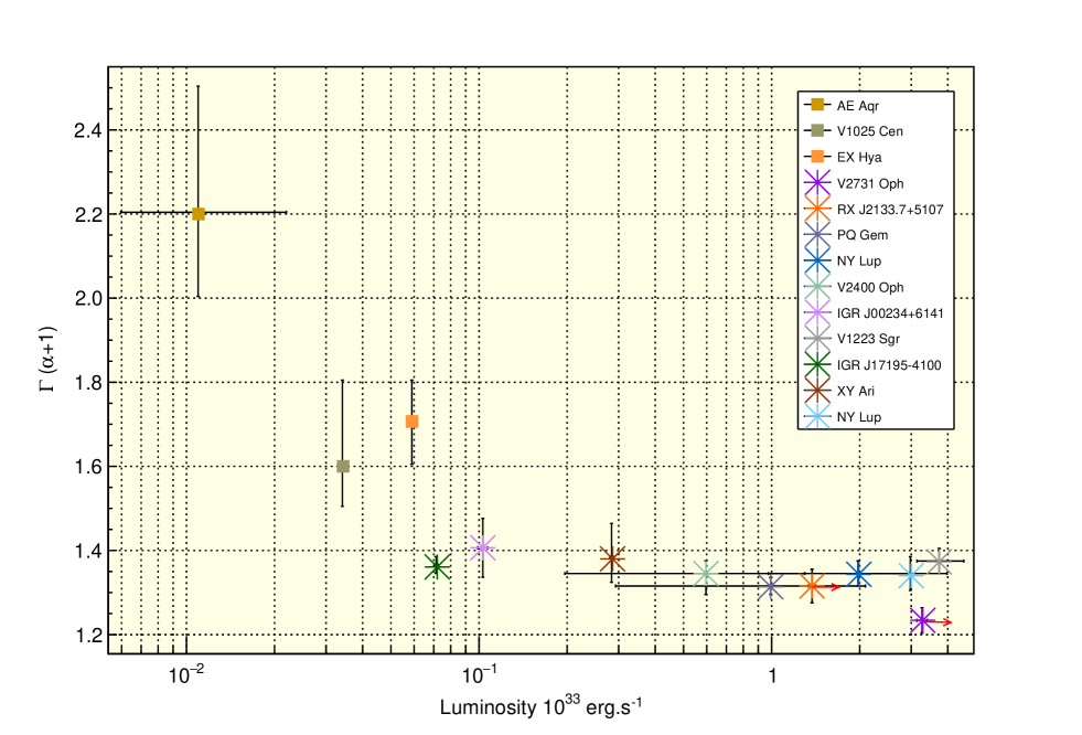
Figure 5: Photon index $\Gamma$ versus luminosity of the unabsorbed Comptonization (CompTT) component in the ($\sim$ 0.3 to 15 keV) energy band (see Table 2 and 5). Red arrow indicates lower limit on the luminosity.

In mCVs a soft X-ray component has been observed in the broad-band X-ray spectrum. This component was discovered by ROSAT and is typically described by a blackbody emission with temperatures ranging from a few up to $\sim$ 100 eV (de Martino et al., 2004, 2006b, 2006a; Mason et al., 1992; Burwitz et al., 1996). In IPs this soft X-ray emission is believed to originate just like in polars, that is, around the accreting poles by the reprocessing of the hard emission on the WD surface (de Martino et al., 2004, 2006b, 2006a). The blackbody fluxes indicate fractional areas of only $\sim 10^{-5}$ of the WD surface for the soft X-ray emission region (Haberl & Motch, 1995). Interestingly, not all IPs show this blackbody component. Evans & Hellier (2007), performing a systematic spectral analysis of XMM-Newton data, stated that this soft blackbody is likely a common component in the X-ray spectra of IPs, suggesting that the lack of the observation of this component can in general be explained by geometrical effects. Namely, depending on the system inclination and the magnetic colatitude (see their Figure 5), the polar region and hence the blackbody component could be hidden by the accretion curtain.

In this standard spectral modelling, the X-ray emission can appear highly absorbed within the accretion flow (with $N_{H}\sim 10^{23}$ cm^-2). Therefore, fits including an extra cold medium totally covering the source or partially ionized covering absorbers (which varies with the orbital phase) are commonly found in the literature (see, e.g., Norton & Watson, 1989; Ishida et al., 1994; Landi et al., 2009). A reflection component (from the WD surface) is also expected and used in the spectral modelling of IPs (see, e.g., Cropper et al., 1998; Beardmore et al., 2000).

Fluorescent Fe $K_{\alpha}$ lines have been observed in most of the IPs (see, e.g., Norton et al., 1991; Ishida, 1991; Hellier et al., 1998; Xu et al., 2016). The moderate spectral resolution of instruments on board Chandra, XMM-Newton  and Suzaku shows that usually up to three emission lines are present in the $\sim$ 6.4 – 7.0 keV range of the spectra. These lines are usually modeled by simple Gaussian components and their centroid energies usually correspond to the cold (neutral) fluorescent Fe $K_{\alpha}$ line at 6.4 keV, and the He- and H-like Fe lines at 6.7 and 7.0 keV, respectively. It is important to notice, however, that more complex line profiles have been reported in these sources (see, e.g., Ishida et al., 1992; Titarchuk et al., 2009). In this standard framework, these lines are believed to be produced by irradiation (or reflection) of hard X-rays on material present on the star surface or somewhere in the accretion flow near the compact object: in the pre-shock material – this interpretation is based on the observation of Doppler-shifted red-wing (redshifted) line in e.g., GK Per – and/or in the lower velocity base of the accretion columns – this interpretation is based on the absence of Doppler shifts in the H- and He-like components (Hellier & Mukai, 2004).

As one can clearly see, the Comptonization process is not the standard one which has been used to describe the X-ray continuum of IPs. We tested if the thermal Comptonization could successfully describe the X-ray continuum of these sources based on the following points: (1) the standard spectral modelling of IPs is found to be similar to nmCVs (2) the continua of nmCVs can be successfully described by thermal Comptonization (Maiolino et al., 2020) (Paper I hereafter) (3) the XMM-Newton Epic pn spectra of the IP GK Per is successfully fitted by the thermal compTT model in XSPEC (Titarchuk et al., 2009), and (4) IPs partially shares geometric/structural similarities with both nmCVs and low mass X-ray binaries (LMXBs).

Accordingly with the catalog of IPs and IP candidates provided by NASA (http://asd.gsfc.nasa.gov/Koji.Mukai/iphome/catalog/alpha.html), eleven out of the 12 IPs present in our sample (AE Aqr, EX Hya, V1025 Cen, V2731 Oph, RX J2133.7+5107, PQ Gem, NY Lup, V2400 Oph, IGR J00234+6141, V1223 Sgr, and XY Ari) are classified as ironclad IPs, while 1 (IGR J17195-4100) is a confirmed IP.

This paper is organized as follows: in section 2 we shortly present the XMM-Newton data reduction, in section 3 we show the results of the spectral analysis, in section 4 we discuss our results, demonstrate some examples of the spectral modelling in the standard framework for some sources in our sample, and present the new thermal Comptonization modelling for IPs. Finally, in section 5 we summarize our main results and conclusions.

2 Data Reduction

The XMM-Newton Epic-pn data reduction was performed through the Science Analysis Software SAS version 14.0.0. Table 1 shows the log of the 13 observations present in our sample. All observations are taken in imaging mode, which allows the extraction of spectra and light curves in the 0.3 to 15 keV energy range. All spectra and light curves were extracted strictly following the Users Guide to the XMM-Newton Science Analysis System Team (2014), and the XMM-Newton ABC Guide (Snowden et al., 2014).

Standard filters were applied on the EVL through the evselect task: taking only good events from the PN camera (using #XMMEA_EP), using single and doubles events (i.e. using pattern $\leq 4$) in the energy range selected, and omitting parts of the detector area like border pixels (and columns with higher offset) for which the patter type and the total energy is known with significantly lower precision (using FLAG==0).

We used the SAS task epatplot to check for pile-up. We found that only the observations of AE Aqr and V2400 Oph were affected by pile-up. In these two cases, in order to mitigate this effect, an inner circle of radius equal to 150 physical unity was excised from the source extraction region during data reprocessing.

In the extraction of light curves, the background subtraction was done accordingly through the SAS task epiclccor, which performs corrections at once for various effects affecting the detection efficiency.

We investigated spectral variability in each observation of our sample by computing hardness ratios (HRs) with light curves produced in 3 energy ranges: 0.3 – 5.0 keV, 5.0 – 8.0 keV, and 8.0 – 15.0 keV. We observed significant variation (pulses) only in the 5.0 – 8.0/0.3 – 5.0 HR of EX Hya. In this case we have not observed spectral differences (except for differences in the normalization) when fitting its spectrum with filter in time – that is, not considering the data taken during the time of the peaks in the 5.0 – 8.0/0.3 – 5.0 HR. This result was expected since the pulses are produced by minima in the 0.3 – 5.0 keV light curve.

Therefore, we have considered the total EPIC-pn exposure time in all final spectral analyses. The photon redistribution matrix (rmf) and the ancillary (arf) files were created through the rmfgen and arfgen task, respectively. All spectra were rebinned in order to have at least 25 counts for each background-subtracted channel.

Table 1: Log of the XMM-Newton Epic-pn Observations of IPs in our sample

Source	Obs. ID	Data Mode	Start Time (UTC)	End Time (UTC)	Exp (ks)
AE Aqr	0111180201	Imaging	2001-11-07  23:45:53	2001-11-08  03:38:17	12.3
EX Hya	0111020101	Imaging	2000-07-01  08:07:39	2000-07-01  20:05:10	30.2
V1025 Cen	0673140501	Imaging	2012-01-01  22:50:42	2012-01-02  02:48:30	13.3
V2731 Oph	0302100201	Imaging	2005-08-29  07:05:40	2005-08-29  10:13:31	10.5
RX J2133.7+5107	0302100101	Imaging	2005-05-29  13:32:59	2005-05-29  17:19:24	12.7
PQ Gem	0109510301	Imaging	2002-10-07  23:13:51	2002-10-08  09:07:21	24.9
NY Lup	0105460301	Imaging	2000-09-07  10:43:41	2000-09-07  16:10:31	17.3
NY Lup	0105460501	Imaging	2001-08-24  16:35:06	2001-08-24  20:46:58	13.5
V2400 Oph	0105460601	Imaging	2001-08-30  15:36:48	2001-08-30  19:56:46	13.7
IGR J00234+6141	0501230201	Imaging	2007-07-10  05:58:25	2007-07-10  12:54:50	21.7
IGR J17195-4100	0601270201	Imaging	2009-09-03  06:57:59	2009-09-03  15:51:53	27.6
V1223 Sgr	0145050101	Imaging	2003-04-13  12:40:18	2003-04-13  23:22:08	27.0
XY Ari	0501370101	Imaging	2008-02-14  18:46:45	2008-02-15  04:16:08	25.6

3 Spectral Analysis

The spectral analysis was performed with the xspec astrophysical spectral package (Arnaud, 1996) version 12.8.2. The 0.3 to 15 keV spectral continua were modeled with a soft blackbody component (when required by the data) plus a thermal Comptonization component, modified by a photo-electric absorption (tbabs model in XSPEC) due to the presence of absorber material (hydrogen column $N_{\mathrm{H}}$) in the line of sight of the source.

The blackbody component was modeled by the bbody model in XSPEC, and the Comptonization component was modeled by the thermal compTT model in XSPEC (Titarchuk, 1994; Hua & Titarchuk, 1995; Titarchuk & Lyubarskij, 1995), considering a cylindrical (plane) geometry. In this model, soft seed photons of temperature $kT_{\mathrm{s}}$ are scattered off by electrons present in a hot plasma (Compton cloud) with temperature $kT_{\mathrm{e}}$ and Thomson optical depth $\tau$.

When residuals were evident in the $\sim$ 6.4 to 7.0 keV energy range, up to three Gaussian components (named in our analysis as Gaussian₁, Gaussian₂ and Gaussian₃) were added to the total model to account for the neutral, He- and H-like Fe lines usually observed in this energy range. When additional spectral features were observed (mainly in the E $\lesssim$ 2.5 keV band) extra Gaussian components (named in our analysis as Gaussian_A,B,C,…,L.) were added to the total model.

The best-fitting parameters of the continuum and fit quality are shown in Table 2. The Gaussian components of the Fe complex are shown in Table 3, whereas the other lines are shown in Table 4.

Table 2: Spectral analysis using the thermal compTT model to describe the $\sim$ 0.3 to 15.0 keV continuum of the IPs. The Gaussian components are shown in Table 3 and 4.

Component

TBABS

bbody

compTT

$\chi^{2}_{\mathrm{red}}$/d.o.f

$\Delta$$E^{f}$ (keV)

Parameters

$N_{\mathrm{H}}$ (1022a)

kTbb (keV)

normg

kTs (keV)

kTe (keV)

$\tau$

normg

Source

AE Aqr

$5.37\times 10^{-2}$b

$0.060_{-0.011}^{+0.002}$

$2.0_{-c}^{+0.5}$

$5.9_{-0.8}^{+0.1}$

$7.3_{-1.3}^{+0.2}$

1.19/549

$0.3-15$

EX Hya

$0.28_{-0.05}^{+0.04}$

$0.089_{-0.003}^{+0.003}$

$22_{-4}^{+6}$

$0.10^{b}$

$3.05_{-0.14}^{+0.17}$

$6.35_{-0.26}^{+0.26}$

$26.7_{-0.8}^{+0.8}$

1.18/1726

$1.0-15$

V1025 Cen

0.01${}_{-c}^{+0.03}$

$0.181_{-0.029}^{+0.014}$

$3.1_{-0.3}^{+0.6}$

$7.1_{-0.7}^{+0.5}$

$2.5_{-0.4}^{+0.4}$

1.15/398

$0.3-15$

V2731 Oph

$0.156^{b}$

$0.018_{-0.003}^{+0.004}$

$3.20_{-0.18}^{+0.22}$

$12.6_{-0.4}^{+0.4}$

$2.51_{-0.11}^{+0.11}$

1.06/696

$1.0-15$

RX J2133.7+5107

$0.134_{-0.013}^{+0.013}$

$0.105_{-0.002}^{+0.003}$

$0.175_{-0.023}^{+0.027}$

$0.17_{-0.08}^{+0.04}$

$3.30_{-0.19}^{+0.23}$

$10.4_{-0.4}^{+0.4}$

$1.95_{-0.15}^{+1.00}$

1.12/1047

$0.3-15$

PQ Gem

$0.033^{b}$

$0.13_{-c}^{+0.04}$

$2.72_{-0.08}^{+0.09}$

$11.69_{-0.24}^{+0.23}$

$2.40_{-0.19}^{+1.05}$

0.96/1461

$0.5-15$

V2400 Oph

$0.004_{-c}^{+0.007}$

$0.108_{-0.011}^{+0.010}$

$2.37_{-0.08}^{+0.08}$

$11.8_{-0.3}^{+0.3}$

$7.2_{-0.3}^{+0.3}$

1.04/1235

$0.3-15$

IGR J00234+6141

0.167${}_{-0.011}^{+0.011}$

0.134${}_{-0.014}^{+0.013}$

$2.84_{-0.21}^{+0.26}$

9.8${}_{-0.5}^{+0.6}$

$0.87_{-0.07}^{+0.06}$

0.92/725

$0.3-15$

IGR J17195-4100

0.091${}_{-0.006}^{+0.006}$

$0.100_{-0.014}^{+0.013}$

2.73${}_{-0.07}^{+0.07}$

10.64${}_{-0.20}^{+0.20}$

$4.88_{-0.21}^{+0.27}$

1.13/1703

$0.3-15$

XY Ari

$4.29_{-0.17}^{+0.23}$

0.1b

4.29${}_{-0.28}^{+0.41}$

$8.0_{-0.6}^{+0.5}$

$2.13_{-0.05}^{+0.05}$

1.12/837

$0.3-15$

V1223 Sgr

$0.51_{-0.05}^{+0.05}$

$0.10_{-0.01}^{+0.01}$

$2.2_{-0.6}^{+0.1}$

0.109b

$2.97_{-0.09}^{+0.10}$

$10.0_{-0.3}^{+0.3}$

$10.8_{-0.2}^{+0.2}$

1.06/1870

$1.0-15$

NY Lupd

$0.100_{-0.013}^{+0.010}$

$0.095_{-0.004}^{+0.003}$

$0.1186_{-0.0013}^{+0.0012}$

$0.068_{-0.006}^{+0.007}$

$3.13_{-0.13}^{+0.15}$

$10.28_{-0.28}^{+0.28}$

$3.46_{-0.03}^{+0.03}$

1.02/1373

$0.3-15$

NY Lupe

0.218b

$0.084_{-0.002}^{+0.002}$

$0.95_{-0.05}^{+0.06}$

$0.021_{-0.004}^{+0.004}$

$3.9_{-0.3}^{+0.3}$

$9.1_{-0.3}^{+0.3}$

$5.7_{-0.4}^{+0.3}$

1.04/1281

$0.5-15$

• Uncertainties at 90% confidence level

• atoms.cm^-2

• Parameter frozen

• Parameter pegged at hard limit

• Obs. ID 0105460301

• Obs. ID 0105460501

• Spectral energy range

• $\times 10^{-03}$

Table 3: Gaussian components present in the $\sim 6.4-7.0$ keV energy range of the Fe emission line complex.

	Gaussian1					Gaussian2					Gaussian3
	E1	$\sigma_{1}$	norm${}_{1}^{e}$	EW1		E2	$\sigma_{2}$	norm${}_{2}^{e}$	EW2		E3	$\sigma_{3}$	norm${}_{3}^{e}$	EW3
Source
AE Aqr						$6.690_{-0.027}^{+0.026}$	$0.05^{+0.04}_{-c}$	$1.5_{-0.3}^{+0.3}$	$821_{-60}^{+431}$
EX Hya	$6.39_{-0.02}^{+0.02}$	$0.02^{b}$	$3.1_{-0.6}^{+0.6}$	$24_{-5}^{+6}$		$6.659_{-0.003}^{+0.003}$	$0.04^{b}$	$33.7_{-1.0}^{+1.0}$	$350_{-11}^{+13}$		$6.96_{-0.01}^{+0.01}$	$0.02^{b}$	$12.1_{-0.7}^{+0.7}$	$108_{-6}^{+8}$
V1025 Cen						6.78${}_{-0.04}^{+0.04}$	0.17${}_{-0.04}^{+0.04}$	4.5${}_{-0.9}^{+0.9}$	$324_{-67}^{+83}$
V2731 Oph	$6.42_{-0.10}^{+0.08}$	$0.39_{-0.11}^{+0.12}$	$10.5_{-2.2}^{+2.5}$	$472_{-92}^{+102}$
RX J2133.7+5107	$6.431_{-0.022}^{+0.023}$	$0.11_{-0.03}^{+0.03}$	$7_{-1}^{+1}$	$268_{-31}^{+238}$							$6.89_{-0.04}^{+0.04}$	$0.07^{b}$	$2.2_{-0.7}^{+0.7}$	$93_{-26}^{+77}$
PQ Gem	$6.38_{-0.02}^{+0.04}$	$0.10_{-0.04}^{+0.06}$	$4_{-1}^{+1}$	$154_{-32}^{+74}$		$6.66_{-0.03}^{+0.04}$	$0.02^{b}$	$1.9_{-1.0}^{+0.6}$	$63_{-23}^{+38}$		$6.94_{-0.03}^{+0.03}$	$0.0c2^{b}$	$1.5_{-0.4}^{+0.4}$	$58_{-16}^{+31}$
V2400 Oph	$6.39_{-0.02}^{+0.04}$	$0.07_{-0.06}^{+0.06}$	$10_{-2}^{+3}$	$150_{-35}^{+93}$		$6.7_{-0.04}^{+0.06}$	$0.07^{b}$	$7_{-2}^{+2}$	$95_{-30}^{+36}$		$6.96_{-0.03}^{+0.04}$	$0.07^{b}$	$5.6_{-1.5}^{+1.4}$	$98_{-29}^{+32}$
IGR J00234+6141						6.70${}_{-0.05}^{+0.05}$	0.23${}_{-0.04}^{+0.05}$	2.7${}_{-0.5}^{+0.4}$	$386_{-9}^{+13}$
IGR J17195-4100	$6.39_{-0.02}^{+0.02}$	$0.07^{b}$	$5.2_{-0.7}^{+0.3}$	$54_{-12}^{+6}$		$6.70_{-0.02}^{+0.03}$	$0.07^{b}$	$2.9_{-0.7}^{+0.3}$	$119_{-19}^{+20}$		$6.97_{-0.02}^{+0.03}$	$0.07^{b}$	$2.9_{-0.6}^{+0.6}$	$81_{-15}^{+17}$
XY Ari	$6.43_{-0.05}^{+0.05}$	$0.07^{b}$	$1.6_{-0.6}^{+0.7}$	$63_{-27}^{+47}$		6.68${}_{-0.04}^{+0.04}$	$0.07^{b}$	$2.4_{-0.7}^{+0.7}$	$103_{-26}^{+69}$		$7.00_{-0.04}^{+0.04}$	$0.07^{b}$	$1.4_{-0.5}^{+0.6}$	$66_{-23}^{+45}$
V1223 Sgr	$6.40_{-0.01}^{+0.01}$	$0.02^{b}$	$9.4_{-0.8}^{+0.8}$	$88_{-8}^{+9}$		$6.68_{-0.01}^{+0.01}$	$0.02^{b}$	$8.2_{-0.8}^{+0.8}$	$73_{-7}^{+8}$		$6.96_{-0.02}^{+0.02}$	$0.05^{b}$	$6.9_{-0.8}^{+0.9}$	$71_{-9}^{+9}$
NY Lupc	$6.38_{-0.02}^{+0.02}$	$0.07$b	$5.1_{-0.7}^{+0.7}$	$145_{-25}^{+29}$		$6.67_{-0.03}^{+0.03}$	$0.07$b	$4.2_{-0.7}^{+0.7}$	$111_{-21}^{+27}$		$6.94_{-0.03}^{+0.03}$	$0.07$b	$3.6_{-0.7}^{+0.7}$	$112_{-25}^{+29}$
NY Lupd	$6.37_{-0.02}^{+0.02}$	$0.07^{b}$	$5.5_{-0.9}^{+0.9}$	$132_{-23}^{+21}$		$6.68_{-0.02}^{+0.02}$	$0.07$b	$6.4_{-0.9}^{+0.9}$	$139_{-23}^{+25}$		$6.97_{-0.02}^{+0.02}$	$0.04^{b}$	$5.5_{-0.8}^{+0.8}$	$120_{-20}^{+23}$

• Uncertainties at 90% confidence level

• Parameter frozen

• Parameter pegged at hard limit

• Obs. ID 0105460301

• Obs. ID 0105460501

• $\times 10^{-5}$

Table 4: Other lines observed in the spectrum the IPs in our sample.

Component	Parameter	Unit	AE Aqr	EX Hya	V1025 Cen	PQ Gem	V2400 Oph	IGR J17195-4100	NY Lupa	NY Lupb
GaussianA	EA	keV				0.52${}_{-0.02}^{+0.02}$		$0.57_{-0.01}^{+0.01}$
	$\sigma_{A}$	keV				$0.10_{-0.02}^{+0.02}$		$0.05_{-0.02}^{+0.02}$
	EWA	eV				$492_{-75}^{+59}$		$54_{-12}^{+6}$
GaussianB	EB	keV	$0.83_{-0.01}^{+0.01}$		0.844${}_{-0.012}^{+0.012}$	$0.89_{-0.02}^{+0.02}$	0.808${}_{-0.014}^{+0.016}$
	$\sigma_{B}$	keV	$0.17_{-0.01}^{+0.01}$		$0.02^{c}$	$0.08_{-0.04}^{+0.06}$	0.059${}_{-0.023}^{+0.023}$
	EWB	eV	$608_{-127}^{+4}$		$24_{-6}^{+7}$	$57_{-10}^{+50}$	-34${}^{+12}_{-13}$
GaussianC	EC	keV		$1.107_{-0.007}^{+0.007}$	1.015${}_{-0.018}^{+0.014}$				$0.98_{-0.02}^{+0.02}$	$0.99_{-0.04}^{+0.03}$
	$\sigma_{C}$	keV		$0.02^{c}$	0.077${}_{-0.015}^{+0.018}$				$0.10_{-0.02}^{+0.02}$	$0.15_{-0.02}^{+0.03}$
	EWC	eV		$15_{-2}^{+3}$	$63_{-12}^{+13}$				$59_{-13}^{+13}$	$151_{-27}^{+29}$
GaussianD	ED	keV		$1.344_{-0.008}^{+0.008}$
	$\sigma_{D}$	keV		$0.02^{c}$
	EWD	eV		$14_{-2}^{+2}$
GaussianE	EE	keV		1.473${}_{-0.005}^{+0.005}$
	$\sigma_{E}$	keV		$0.02^{c}$
	EWE	eV		$24_{-2}^{+3}$
GaussianF	EF	keV		$1.848_{-0.008}^{+0.010}$
	$\sigma_{F}$	keV		$0.02^{c}$
	EWF	eV		$20_{-3}^{+3}$
GaussianG	EG	keV		$1.995_{-0.004}^{+0.006}$	1.98${}_{-0.04}^{+0.04}$
	$\sigma_{G}$	keV		$0.005^{c}$	$0.075^{c}$
	EWG	eV		$28_{-3}^{+2}$	$34_{-11}^{+11}$
GaussianH	EH	keV		$2.444_{-0.012}^{+0.011}$	2.46${}_{-0.03}^{+0.04}$
	$\sigma_{H}$	keV		$0.02^{c}$	$0.02^{c}$
	EWH	eV		$19_{-4}^{+4}$	$38_{-11}^{+12}$
GaussianI	EI	keV		$2.61_{-0.01}^{+0.01}$
	$\sigma_{I}$	keV		$0.02^{c}$
	EWI	eV		$24_{-4}^{+3}$
GaussianJ	EJ	keV		$3.918_{-0.024}^{+0.022}$
	$\sigma_{J}$	keV		$0.024^{c}$
	EWJ	eV		$18_{-4}^{+18}$
GaussianK	EK	keV		$7.82_{-0.02}^{+0.02}$
	$\sigma_{K}$	keV		$0.06^{c}$
	EWK	eV		$88_{-12}^{+14}$
GaussianL	EL	keV		$8.21_{-0.03}^{+0.02}$
	$\sigma_{L}$	keV		$0.02^{c}$
	EWL	eV		$46_{-12}^{+13}$

• Uncertainties at 90% confidence level

• Obs. ID 0105460301

• Obs. ID 0105460501

• Parameter frozen

In all fits, the hydrogen column density $N_{\mathrm{H}}$ was first fixed to the value given by the HI4PI survey (HI4PI Collaboration et al., 2016). However, in nine observations (in EX Hya, V1025 Cen, RX J2133.7+5107, V2400 Oph, IGR J00234+6141, IGR J17195-4100, XY Ari, V1223 Sgr, and NY Lup Obs. ID 0105460301) a satisfactory fit was attained only when this parameter was set to vary freely.

We noticed that the presence of complex residuals in the soft $\sim$ 0.3 – 1.0 keV band in EX Hya, V2731 Oph and V1223 Sgr worsened the fit quality. These residuals are likely caused by the contribution of a forest of emission lines in this band. In V1223 Sgr, for example, lines likely from O VII at 0.574 keV and N VII at $\sim$ 0.5 keV are evident. We observed that the modelling of these features (with Gaussian components) does not strongly affect the best-fitting parameters of the continuum (compTT component), and hence we did not consider this soft energy range in our final fit.

The presence of the soft bbody component is necessary in our total spectral modelling of EX Hya, RX J2133.7+5107, V1223 Sgr and NY Lup. In EX Hya, RX J2133.7+5107 and NY Lup spectra a fit with reduced $\chi^{2}$($\chi^{2}_{\mathrm{red}}$) $<$ 2.0 is attained only if this component is present. For the other observations we checked the presence of this extra component by means of the F-test defined in terms of the ratio between the normalized $\chi^{2}$(e.g, Maiolino et al., 2020, and references therein). In V1223 Sgr the probability of chance improvement (PCI) when adding the extra component is marginal, equal to $1.7\times 10^{-3}$. However, when the fit is performed in the total 0.3 – 15 keV energy band the presence of the soft bbody component is more evident, with PCI of $9\times 10^{-5}$ or even lower ($\sim 10^{-19}$) depending on the modelling of the strong and complex residual excesses present in the soft $\sim$ 0.5 – 1.2 keV energy band. Therefore we decided to keep the bbody component in our final total modelling.

Interestingly, in the analysis of PQ Gem, a bbody component of $kT_{\mathrm{s}}$ of 88${}^{+4}_{-3}$ eV is apparently present at first, with PCI of $2.2\times 10^{-91}$. However, in this case strong residuals remain in the soft energy band (E $<$ 1 keV), and when Gaussian components are included to take these residuals into account the new PCI for the bbody is equal to 42%. Therefore, in this case we did not consider the soft bbody component in our final total modelling.

Figure 1 shows the best spectral fits in AE Aqr, V1025 Cen, and HX Hya. Figure 2 shows the best spectral fits in V2731 Oph, RX J2133.7+5107, PQ Gem, and V2400 Oph. Figure 3 shows the best spectral fits in IGR J00234+6141, IGR 17195-4100, XY Ari and V1223 Sgr. Finally, Figure 4 shows the best spectral fits in NY Lup Obs. 0105460301 and 0105460501, respectively.

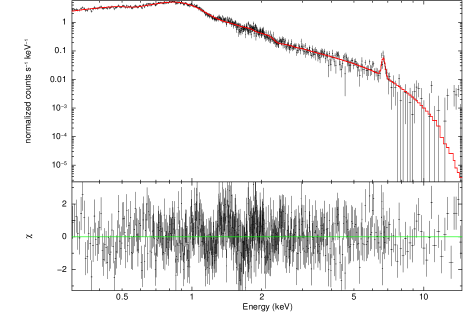
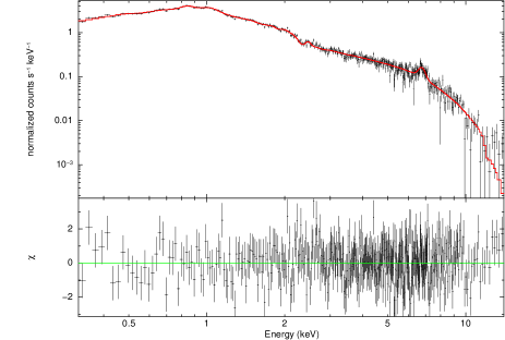
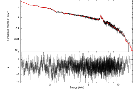
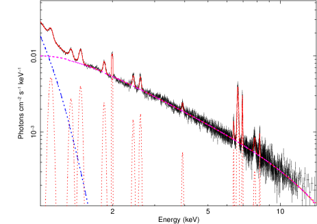
Figure 1: XMM-Newton EPIC pn spectra (in black) and the best fit total model (solid red line). Left top panel: spectrum of AE Aqr in the 0.3 – 15.0 keV energy range, and the best fit total model tbabs*[compTT+(2)gaussian components]. Right top panel: spectrum of V1025 in the 0.3 – 15.0 keV energy range, and the best fit total model tbabs*[compTT+(5)gaussian components]. Left lower panel: spectrum of EX Hya in the 1.0 – 15.0 keV energy range, and the best fit total model tbabs*[compTT+(13)gaussian components]. Right lower panel: unfolded spectrum of EX Hya in the 1.0 – 15.0 keV energy range; the total model in red, the bbody component in blue, the compTT component in magenta, and the Gaussian components in dashed red lines. See Table 2, 3, and 4.

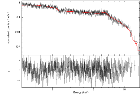
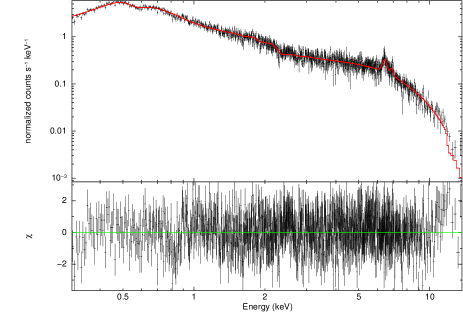
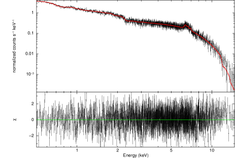
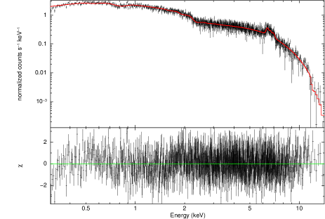
Figure 2: XMM-Newton EPIC pn spectra (in black) and the best fit total model (solid red line). Left top panel: spectrum of V2731 Oph in the 1.0 – 15.0 keV energy range, and the best fit total model tbabs*[compTT+gaussian]. Right top panel: spectrum of RX J2133.7+5107 in the 0.3 – 15.0 keV energy range, and the best fit total model tbabs*[compTT+(2)gaussian components]. Left lower panel: spectrum of PQ Gem in the 0.5 – 15.0 keV energy range, and the best fit total model tbabs*[compTT+(5)gaussian components]. Right lower panel: spectrum of V2400 Oph in the 0.3 – 15.0 keV energy range, and the best fit total model tbabs*[compTT+(4)Gaussian components]. See Table 2, 3, and 4.

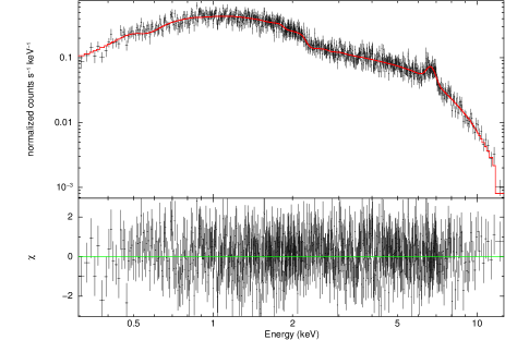
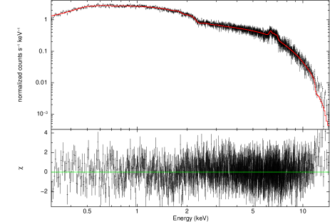
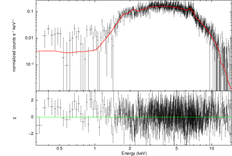
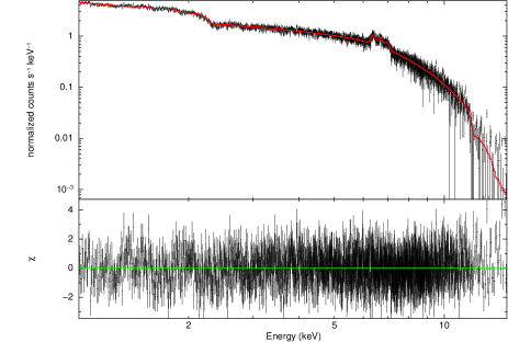
Figure 3: XMM-Newton EPIC pn spectra (in black) and the best fit total model (solid red line). Left top panel: spectrum of IGR J00234+6141 in the 0.3 – 15.0 keV energy range, and the best fit total model tbabs*[compTT+gaussian]. Right top panel: spectrum of IGR 17195-4100 in the 0.3 – 15.0 keV energy range, and the best fit total model tbabs*[compTT+(4)gaussian components]. Left lower panel: spectrum of XY Ari in the 0.3 – 15.0 keV energy range, and the best fit total model tbabs*[compTT+(3)gaussian components]. Right lower panel: spectrum of V1223 Sgr in the 1.0 –15.0 keV energy range, and the best fit total model tbabs*[compTT+(3)gaussian components]. See Table 2, 3, and 4.

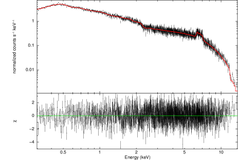
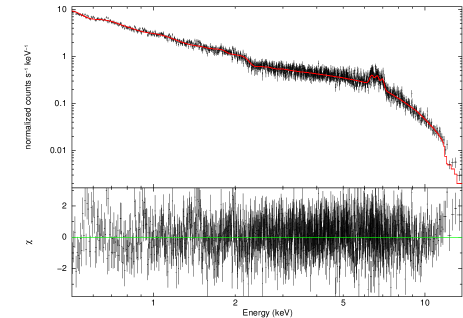
Figure 4: XMM-Newton EPIC pn spectra (in black) and the best fit total model (solid red line). Left panel: spectrum of Obs. ID 0105460301 in the 0.3 –15.0 keV energy range, and the best fit total model tbabs*[compTT+(4)gaussian components]. Right panel: spectrum of Obs. ID 0105460501 in the 0.5 –15.0 keV energy range, and the best fit total model tbabs*[compTT+(4)gaussian components]. Table 2, 3, and 4.

Spectral lines

For each spectrum, we investigated the presence of each Gaussian component by means of the simftest script in xspec. The probability that data are consistent with the total model without considering each of these components (shown in Table 3 and 4) is low – compatible with zero.

In eight out of the thirteen spectra present in our sample we observed all the three emission lines of the $\sim$ 6.4 – 7.0 keV Fe complex (in EX Hya, PQ Gem, V2400 Oph, IGR J17195-4100, XY Ari, V1223 Sgr, and in both observations of NY Lup; see Table 3). In these observations (a) in general, the Gaussian₁ component is compatible, within errors, with the neutral Fe $K_{\mathrm{\alpha}}$ line at 6.4 keV; only NY Lup Obs. ID 0105460501 shows a Gaussian₁ centroid energy at 1.5 $\sigma$ from the neutral Fe $K_{\mathrm{\alpha}}$ (b) in general, the centroid energy of the Gaussian₂ component is compatible, within errors, with the He-like Fe line at 6.7 keV and/or 6.675 keV; EX Hya shows a Gaussian₂ with centroid energy at 13 $\sigma$ (due to the small error bar) and 5.3 $\sigma$ from the 6.7 and 6.675 keV lines, respectively, and V1223 Sgr shows a Gaussian₂ line at 2 $\sigma$ from the 6.7 keV line; and (c) only V2400 Oph, IGR J17195-4100 and XY Ari show a Gaussian₃ component with centroid energy compatible, within errors, with the H-like Fe line at 7.0 keV; PQ Gem, V1223 Sgr and NY Lup Obs. ID 0105460301 show Gaussian₃ centroid energy at 2 $\sigma$ from this line, while HX Hya and NY Lup Obs. ID 0105460501 show centroid energies at 4 $\sigma$ and 1.5 $\sigma$, respectively.

In RX J2133.7+5107 we only observed the Gaussian₁ and Gaussian₃ components. The centroid energy of the Gaussian₁ (appears blue-shifted) at 1.4 $\sigma$ from the neutral Fe line, while the centroid energy of the Gaussian₃ (appears red-shifted) at 2.75 $\sigma$ from the H-like Fe line. In V1025 Cen, AE Aqr and IGR J00234+6141 spectra, we observed only the Gaussian₂ component, which appears in general compatible with the He-like Fe line. Only V1025 Cen shows a centroid Gaussian energy apparently blue-shifted at 2 $\sigma$ from the He-like Fe line. However, the peak of this feature is exactly at 6.7 keV.

Finally, the V2731 spectrum shows only a broad Gaussian₁ component, with centroid energy compatible with neutral Fe line (see Table 3).

AE Aqr, EX Hya, V1025 Cen, PQ Gem, V2400, IGR J17195-4100 and the two observations of NY Lup show lines other than the Fe lines in the 6.4 – 7.0 keV energy range (see Table 4). These features are present mainly in the soft X-ray spectra (E $\lesssim$ 1.5 – 2.5 keV).

In AE Aqr, we observed a strong and relatively broad excess in the soft X-ray energy band (from $\sim$ 0.7 to 1.1 keV) peaked at $\sim$ 0.9 keV (this peak is compatible with either Ne IX, Ni XIX, Ca XVII, or Fe XIX ion transitions). This feature, identified as Gaussian_B component in Table 4, has a centroid energy at 0.83${}_{-0.01}^{+0.01}$ keV, which is compatible with line emission from Fe XVII ion at 0.826 keV, or Fe XIX at 0.823 keV. This source still show residual trends in the E $<2.5$ keV energy range (see Figure 1, left top panel), which may have contributed for a worse spectral fit quality in this source. These residuals are peaked at $\sim$ 1.4 keV, 1.9 keV and 2.4 keV, which could possibly be produced by line emissions from Mg, Si and S ions, respectively.

V2400 Oph shows an absorption line, identified as Gaussian_B component in Table 4. This line shows a centroid energy at 0.808${}^{+0.016}_{-0.014}$ keV, which could be absorption of either Ca XVII (at 0.8 keV), Fe XVI (at 0.805 keV), Fe XVII (at 0.802 or 0.812 keV), or Fe XIX (at 0.823 or 0.819 keV) photons. It is important to stress, however, that this centroid energy is close, within errors, to the Fe XVII line energy at 0.826 keV, which is (as previously stated) possibly present in the spectra of AE Aqr as well.

As in AE Aqr, PQ Gem shows a residual excess peaked at $\sim$ 0.9 keV. The modelling of this feature, identified as Gaussian_B component in Table 4, leads to a centroid Gaussian energy at 0.89${}^{+0.02}_{-0.02}$ keV. This Gaussian component is compatible with either Ni XIX (at 0.884 or 0.900 keV) or Ca XVIII (at 0.886 keV) ion line emission, and it is very close to Fe XIX (0.918 keV) and Ne IX (at 0.914 keV) ion line emissions. A strong and broad additional trend, peaked at $\sim$ 0.57 keV, is observed in this source. The energy of this peak is compatible with the resonance O VII line at 0.574 keV, and it is close to the K_α line of O VII at 0.559 keV. However, the modeling of this trend with a symmetric Gaussian (identified as Gaussian_A in Table 4) leads to a centroid energy of 0.52${}^{+0.02}_{-0.02}$ keV, compatible with lines from N VII (at 0.500 keV) and N VI (at 0.522 keV) line emissions, and very close to N VI line emission at 0.498 keV.

IGR J17195-4100 shows only one line emission with peak and centroid Gaussian energy at 0.57${}^{+0.1}_{-0.1}$ keV (see Gaussian_A component in Table 4). In comparison with PQ Gem, this feature appears rather weak.

The two NY Lup spectra show a broad excess peaked at $\sim$ 1.01 – 1.10 keV (with Gaussian centroid energy at $\sim$ 1 keV in both observations). This line is compatible with Ne X (at 1.022 keV), Fe XVII (at 0.976 and 1.023 keV), Fe XX (at 0.992 and 1.008 keV) and Fe XXI (at 1.008 keV) line emission. It appears stronger in Obs. ID 0105460501 than in Obs. ID 0105460301 (see Gaussian_C component in Table 4).

The source V1025 Cen shows four line emissions, identified as Gaussian_B, Gaussian_C, Gaussian_G and Gaussian_H in Table 4. The centroid energy of Gaussian_B is at 1.5 $\sigma$ from the Fe XVII line emission at 0.826 keV. Gaussian_C is compatible within errors with NeX and Fe XXI line emissions at 1.022 and 1.008 keV, respectively. Gaussian_G is compatible within errors with Si XIV line emission at 2.007 keV. Finally, Gaussian_H agrees perfectly with S XV line emission at 2.460 keV.

Apart from the Fe line complex, the source EX Hya shows ten line emissions, identified by Gaussian_C,..,L components in Table 4. Gaussian $D$, $E$, $J$, and $L$, agree within errors with Ni XXVI (at 1.348 keV), Mg XII (at 1.473), Ca XIX (at 3.903 keV), and Fe XXVI (at 8.212 keV) line emissions, respectively. Whereas, Gaussian C, F, G, H, I, and K, is at 2.3, 1.7, 2.0, 1.45, 1.3, and 1.05 $\sigma$, respectively, from the Fe XXIII (1.123 keV), Si XIII (at 1.865 keV), Si XIV (at 2.007 keV), S XV (at 2.460 keV), S XVI (at 2.623 keV), and Ni XXVII (at 7.799 keV) line emissions, respectively.

4 Discussion

Following Paper I, in this paper we tested if the thermal Comptonization could describe the X-ray continuum of IPs. We obtained that the thermal compTT model can, in general, successfully describe the XMM-Newton Epic-pn average continuum of the IPs in our sample. In all 13 observations we obtained $\chi^{2}_{\mathrm{red}}$ of $\sim$ 1.0 (see Table 2). However, in five observations we did not obtain a satisfactory fit in the total  0.3 – 15 keV XMM-Newton Epic-pn energy range. In these cases, our total model is not able to account for the more complex and subtleties of the soft (E $\lesssim$ 1 keV) X-ray spectral shape seen in EX Hya, V2731 Oph, V1223 Sgr, PQ Gem and NY Lup Obs. ID 010546050. Our modelling is capable to describe the spectra of V2731 Oph and V1223 Sgr in the 1.0 – 15 keV energy range, and PQ Gem and NY Lup in the 0.5 – 15 keV energy range, respectively – with best-fitting parameters in agreement with the values found for the other sources. The compTT component shows a mean seed photon temperature $<kT_{\mathrm{s}}>$ of 0.096 $\pm$ 0.013 keV, a mean electron temperature $<kT_{\mathrm{e}}>$ in the Compton cloud of 3.05 $\pm$ 0.16 keV, and a mean optical depth $<\tau>$ of 9.5 $\pm$ 0.6.

4.1 Soft X-ray component

We observed an additional soft blackbody (bbody) component in five out of the thirteen spectra in our sample (in EX Hya, RX J2133.7+5107, V1223 Sgr, and NY Lup Obs. ID 0105460301 and Obs. ID 0105460501).

This bbody component shows a mean temperature $<kT_{\mathrm{bb}}>$ of $0.095\pm 0.004$ eV, and it is in general compatible with values reported in the literature. For example, Anzolin et al. (2009) stated the presence of a blackbody with a temperature of $\sim$ 100 eV in the average (using 0.3 – 100 keV XMM-Newton, same Obs. ID present in our sample, and SUZAKU spectra) spectra of RX J2133.7+5107. In our analysis this source showed a blackbody component of $105^{+3}_{-2}$ eV, which is in agreement with the literature. The source NY Lup is another IP well known for showing a soft blackbody X-ray component (Potter et al., 1997). Namely, Haberl et al. (2002) using the same XMM-Newton Epic-pn observation present in our sample, found a blackbody of $\sim$ 84 – 97 eV. A value of $\sim$ 104 eV (Evans & Hellier, 2007; Katajainen et al., 2010) is reported in the literature as well. In our analyses, we found a bbody component of $95^{+3}_{-4}$ eV and $84^{+2}_{-2}$ eV, respectively, in the two observations of NY Lup analysed (see Table 2, line 15 and 16) – which are in agreement with the values reported in the literature.

A soft blackbody component is reported in V2400 Oph as well. For example, de Martino et al. (2004) using BeppoSAX data found a blackbody component of 103 $\pm$ 10 eV, Evans & Hellier (2007) revealed a temperature of $117^{+33}_{-44}$ eV for this component using the same observation present in this paper, and Joshi et al. (2019) showed a blackbody component with an average temperature of $\sim$ 98 eV in the XMM-Newton and SUZAKU spectra. However, in our analysis of V2400 Oph average spectrum a blackbody component was not required by the data. A possible reason for not observing this component could be the different software version used for the data reduction and the different spectral total modelling (framework) used to describe the data. Similarly, in V2731 Oph a blackbody component (of $\sim$ 90 eV) is reported in the literature (de Martino et al., 2008), but we did not find this component in our analysis.

As previously stated, a soft blackbody component was not necessary to describe the XMM-Newton data of PQ Gem in our final modeling (that is, when Gaussian components were added to the total model to account for emission features in E $\lesssim$ 1 keV). The bbody temperature of $88^{+4}_{-3}$ eV found when considering this component is slightly higher than those pointed out in the literature of $\sim$ 50 – 60 eV (see Evans & Hellier, 2007, and references therein; who analysed the same data set in the standard multi plasma temperature framework).

Evans & Hellier (2007), using the standard spectral modelling, did not state the presence of a blackbody component in the spectrum of V1223 Sgr. In our framework, on the other hand, we observed a weak blackbody with temperature of 100 $\pm$ 10 eV when fitting in the 1.0 – 15.0 keV energy range. However, when using the total 0.3 – 15 keV energy band we observed that the temperature of this component is found in the 20 – 40 eV range, which depends on the modelling of the residual soft (E $\lesssim$ 1 keV) X-ray excesses.

Suleimanov et al. (2016) stated that the soft excess in the (XIS + HXD) SUZAKU spectrum of EX Hya can be modelled by either a blackbody or an APEC component with $kT\sim 200$ eV, which is approximately two times of the temperature found by our analysis.

Therefore, we found that the presence and the temperature of this soft X-ray component can depend on the modelling of the lines present in the soft energy range, the total spectral model, and (as expected) the spectral energy range analysed.

4.2 Continuum spectral shape in IPs

In general, the shape of a Comptonization spectrum is composed by four parts: a blackbody hump, a power-law, a high energy tail, and a transition region between the parts.

The energy spectral index $\alpha$ of the spectra in our sample ranges (within errors) from 0.20 to 1.2, with a mean value $<\alpha>$ equal to 0.45 $\pm$ 0.07. Namely, we observed a bimodal space for $\alpha$. In ten observations with the Comptonization parameter $y$ ($y\sim 4kT_{\mathrm{e}}\tau^{2}/m_{\mathrm{e}}c^{2}$) $\gtrsim$ 2 (and $<\tau>$ of 10.4 $\pm 0.4$), we obtained spectral index $<\alpha>$ of $0.34\pm 0.02$. On the other hand, in the three observations (AE Aqr, EX Hya, and V1025 Cen) with $y$ $\lesssim$ 1.0 (and lowest $\tau$ among the sources, with $<\tau>$ equal to $6.5_{-0.4}^{+0.4}$), we obtained the highest $\alpha$, with $<\alpha>$ equal to $0.83\pm 0.19$.

Titarchuk et al. (2009), using the wabs*(compTT+Gaussian) model in XSPEC but different spectral energy range and Compton cloud geometry, found an acceptable spectral fit ($\chi^{2}_{\mathrm{red}}$= 73.6/77 $\sim$ 1.0) to a XMM-Newton spectrum of the IP GK Per. The authors reported higher best-fitting parameters for their thermal compTT component ($kT_{\mathrm{s}}$ equal to 1.05 $\pm$ 0.57 keV, $kT_{\mathrm{e}}$ equal to 5.3 $\pm$ 0.5 keV and $\tau$ equal to 20.9 $\pm$ 1.8; which gives $\alpha$ equal to $0.21^{+0.06}_{-0.04}$). In comparison with our modeling, the different spectral energy band and Compton cloud geometry likely contributed to a difference observed in $kT_{\mathrm{e}}$ and $\tau$ parameters. In particular, if one uses a spherical geometry then the optical depth of the Compton cloud increases. For the sources of our sample, we obtained $<\tau>$ of $\sim$ 20. It is important to stress, however, that different plasma geometry (sphere or plane) does not affect the shape of the resulting spectra.

For optically thick Compton clouds with $\tau\gg 1$ all soft photons illuminating a cloud are Comptonized. Consequently, it can be expected that the power-law portion of the spectrum should be relatively small (or even not present at all), and in this case the emergent spectrum is close to a Wien shape (Hua & Titarchuk, 1995).

The photon index $\Gamma$ ($\Gamma=\alpha+1$) of about $1.30$ found in the majority of the sources in our sample may indicate a spectral dichotomy between nmCVs and the majority of IPs; the photon indices $\Gamma\sim 1.85$ is reported in nmCVs (Paper I) when broadband spectral analysis is considered. The difference between these spectra lies on the fact that the spectra of the IPs with $\Gamma\sim 1.30$ approaches to a Wien shape (Sunyaev & Titarchuk, 1980). This lower photon index is likely caused by the increase in the luminosity, which consequently changes the physical conditions in the Compton cloud (that is, it increases its optical depth).

The sources AE Aqr, EX Hya, and V1025 Cen show $<\Gamma>$ compatible, within errors, with that found in nmCVs. In this case the spectral formation is similar to that in nmCVs.

Table 5 shows the unabsorbed fluxes of our total modeling, the spectral compTT component (from which luminosity has been computed), and the bbody component when present. In Figure 5, despite (a) the large errors on luminosity estimates due to the large errors on distance estimates and (b) the narrow range of physical Comptonization parameters shared by most of the IPs analysed, one can see a negative correlation between $\Gamma$ and L, where $\Gamma$ decreases with increase in L.

Namely, $\Gamma\sim$ 1.3 is found for the sources with luminosity of about $\sim$10³³ erg.s^-1, whereas $\Gamma\sim$ 2 is found for the faint IPs with $\sim$ 10³¹ erg.s^-1. This bimodal spectral (or photon) index observed in Figure 5 follows the bimodal X-ray luminosity L observed in IPs, which demonstrated two peaks at L $\sim 10^{31}$ and $\sim 10^{33}$ erg. s^-1 (Pretorius & Mukai, 2014).

The source AE Aqr has magnetic field ($B_{WD}\sim 10^{6}$ G) in the lower range of IPs, and shows similarities with nmCV spectra: L $\sim 10^{31}$ erg.s^-1, presence of a broad and strong excess in the soft X-ray energy band ($<$ 1 keV) peaked at $\sim$ 0.9 keV (with centroid Gaussian energy at $0.83_{-0.01}^{+0.01}$ keV), and photon index $\Gamma\sim 2$ – all characteristics found in nmCV spectra in the thermal Comptonization framework (Paper I). It is important to notice, however, that strong and broad emission lines peaked at $\sim$ 0.9 – 1.01 keV are also observed in others IPs (see Table 4). Therefore, the high spectral index in the IP AE Aqr, as well as in EX Hya and V1025 Cen, can be related to close physical conditions in faint IPs and nmCVs for X-ray emission in the Compton cloud and X-ray (re)processing in the (in/out)flow in the system. Luna et al. (2010) stated that EX Hya shows spectral features of both magnetic and nmCVs, when analysing the ${\it Chandra}$ spectrum of this source in the standard framework of the post shock region models (see also Mukai et al., 2003).

Comparing the best-fitting parameters of the compTT component found in this present work with those found in nmCVs through XMM-Newton data, we see that the temperature of the electrons in the Compton cloud in IPs is about two (or more) times lower ($kT_{\mathrm{e}}$ ranges from $\sim$ 5.99 to 8.72 keV in nmCVs) while the optical depth (for plane geometry) is around two (or more) times higher ($\tau$ ranges from 2.65 to 4.73 in nmCVs) (Paper I).

It is also important to point out that AE Aqr also shares characteristics with young spin-powered pulsars in the 2 – 20 keV range (see Oruru & Meintjes, 2012). AE Aqr is a peculiar nova-like, which hosts the fastest spinning WD ($P_{\text{spin}}=33$ s) (Wynn et al., 1997), which is spinning down at $\dot{P}_{\text{spin}}=5.64\times 10^{-14}$ s s^-1 rate (van Heerden & Meintjes, 2015, and references therein). Gotthelf (2003) observed that the 2 – 10 keV Chandra spectra of young rotation-powered pulsars show photon indices such that $0.6<\Gamma<2.1$. Interestingly, the nine young rotation-powered pulsars studied by them showed mean photon index $<\Gamma>\sim 1.4$, which is close to the mean value found in this study for IPs.

4.3 Some examples of previous spectral analyses and comparison with our results

The standard spectral modelling of IPs is not homogeneous. That is, their spectra have been described by either up to three optically thin plasma temperatures or cooling flow models – exactly like in nmCVs. For example, the emission component $\leq$10 keV of AE Aqr has been fitted by multi-temperature models (Terada et al., 2008; Oruru & Meintjes, 2012). Terada et al. (2008) using Suzaku data, fitted the X-ray spectra of AE Aqr using multi-thermal components, with temperatures of $2.9^{+0.20}_{-0.16}$ keV and $0.53^{+0.13}_{-0.14}$ keV. The excess above the extrapolated hard X-ray emission data was explained by either a third thermal component of $54^{+0.26}_{-0.47}$ keV or a power law with a photon index of 1.12${}^{+0.63}_{-0.62}$. de Martino et al. (2008) described the 0.2 – 100 keV XMM-Newton and INTEGRAL spectra of V2731 Oph by multi-temperature thermal plasma with temperature ranging from 0.17 to 60 keV (plus a hot blackbody of $\sim$90 eV, as previously stated). Anzolin et al. (2009) modeled the 0.3 to 100 keV XMM-Newton and INTEGRAL average spectra of RX J2133.7+5107 and IGR J00234+6141 (their data sample contains the same XMM-Newton Epic pn observations presented in this paper). In addition to the optically thick blackbody component of $\sim$ 100 eV (previously mentioned), the authors described the spectra by means of (a) 2 and (b) 3 different mekal components, and (c) by a multi-temperature cemekl. For the fit considering two mekal components, the authors found a low (kT $\sim$ 0.17 keV) and an intermediate temperature (kT $\sim$ 10 keV). The additional third component shows kT $>$ 27 keV. For the cooling flow cemekl model the authors stated a maximal cemekl temperature in the 40 to 95 keV range (see Table 4 and 5 in Anzolin et al., 2009).

Haberl et al. (2002), using the same XMM-Newton EPIC observation of NY Lup presented in our sample (Obs. ID 0105460301), fitted a multi-temperature plasma component to the 0.1–12 keV NY Lup spectrum, and stated a maximum temperature of $\sim$ 60 keV. Joshi et al. (2019) used two MEKAL components, with $kT_{1}\sim$ 7 and $kT_{2}\sim$ 26 keV, to explain the 0.3 – 50 keV SUZAKU spectra of V2400 Oph; and one MEKAL component with $kT\sim$ 10 keV to describe the XMM-Newton  spectra. Xu et al. (2016) using SUZAKU data fitted a single thermal plasma temperature apec model to the 2 – 10 keV continuum of several IPs. They stated a plasma temperature of $65.9_{-13.3}^{+18.3}$ keV in RX J2133.7+5107, $32.6^{+12.7}_{-7.11}$ keV in PQ Gem, $43.5_{-7.53}^{+11.76}$ keV in NY Lup, $22.8^{+2.01}_{-1.78}$ keV in V2400 Oph, $26.6^{+4.40}_{-3.47}$ keV in V1223 Sgr, $30.5^{+8.94}_{-6.06}$ keV in IGR J17195-4100, and $39.6^{+13.1}_{-8.21}$ and $31.6^{+13.1}_{-8.46}$ keV in XY Ari, respectively.

In comparison with the standard scenario, when only one optically thin thermal plasma temperature is used, the Comptonization model can give temperatures $\sim$ 10 times lower (when they are determined applying the 0.3 – 15 keV XMM-Newton spectra).

In our spectral modeling we used only a simple photoeletric absorption component. The presence of dense absorber material partially covering the X-ray source is not required. In the standard framework, however, one or more partial covering absorbers components are commonly necessary in the total modelling for a good description of the data (see section 1). For example, in V2400 Oph and NY Lup about $\sim$ 50% of the X-ray source is stated to be partially covered by a dense absorber (see, e.g., Haberl et al., 2002; Evans & Hellier, 2007; Joshi et al., 2019). On the contrary, we see in our modelling that in 6 out of 13 observations the hydrogen column component is attenuated by a $\sim$ 2 – 20 factor. Only in three spectra (in EX Hya, XY Ari and V1223 Sgr; see Table 2), the average spectra are absorbed by denser hydrogen column, which indicates to the presence of interviewing dense material likely located somewhere within or close to the system. In 4 observations we obtained satisfactory fits by setting and freezing the hydrogen column $N_{\mathrm{H}}$ parameter equal to the value given by the HI4PI survey.

Table 5: Unabsorbed flux found for our total modelling, the compTT and bbody components (in the $\sim$ 0.3 to 15 keV; see Table 2,3,4).

Source	Flux (total)	Flux (compTT)	Flux (blackbody)	Distance	Refs
	$10^{-11}$ erg.cm-2.s-1	$10^{-11}$ erg.cm-2.s-1	$10^{-11}$ erg.s-1.cm-2	pc
AE Aqr	1.088${}^{+0.021}_{-0.011}$	$0.859^{+0.011}_{-0.009}$		$102^{+42}_{-23}$	1
EX Hya	13.56${}^{+0.03}_{-0.03}$	11.85${}^{+0.04}_{-0.04}$	0.707${}^{+0.011}_{-0.011}$	64.5${}^{+1.2}_{-1.2}$	2
V1025 Cen	2.481${}^{+0.022}_{-0.022}$	2.374${}^{+0.026}_{-0.026}$		110	2
V2731 Oph	2.85${}^{+0.11}_{-0.10}$	$2.75^{+0.11}_{-0.11}$		$>1000$	2
RX J2133.7+5107	4.25${}^{+0.08}_{-0.08}$	$3.22^{+0.08}_{-0.10}$	$0.94^{+0.03}_{-0.04}$	$>$600	3
PQ Gem	3.27${}^{+0.06}_{-0.06}$	$3.05^{+0.02}_{-0.02}$		510${}^{+280}_{-180}$	2
NY Lupa	4.62${}^{+0.05}_{-0.05}$	$3.89^{+0.08}_{-0.08}$	$0.57^{+0.008}_{-0.008}$	$690^{+150}_{-150}$	4
NY Lupb	9.33${}^{+0.05}_{-0.05}$	$5.20^{+0.04}_{-0.04}$	$3.85^{+0.05}_{-0.05}$
V2400 Oph	6.48${}^{+0.13}_{-0.12}$	$6.63^{+0.05}_{-0.05}$		$280^{+150}_{-100}$	2
IGR J00234+6141	$0.99^{+0.04}_{-0.04}$	$0.96^{+0.04}_{-0.04}$		$300$	5
IGR J17195-4100	$5.16^{+0.05}_{-0.05}$	$5.01^{+0.07}_{-0.07}$		$110$	6
XY Ari	$3.34^{+0.04}_{-0.04}$	$3.28^{+0.05}_{-0.05}$			7
V1223 Sgr	$11.9^{+1.1}_{-1.2}$	$11.49^{+0.04}_{-0.04}$	$0.162^{+0.005}_{-0.005}$	$527^{+54}_{-43}$	2,5,8,9

References: 1. Friedjung (1997); 2. Pretorius & Mukai (2014, and references therein); 3. Bonnet-Bidaud et al. (2006); 4. de Martino et al. (2006a); 5. Barlow et al. (2006, and references therein); 6. Masetti et al. (2006); 7. Littlefair et al. (2001); 8. Beuermann et al. (2004); 9. Nwaffiah & Eze (2014).
^a Obs. ID 0105460301.
^b Obs. ID 0105460501.

4.4 The Comptonization scenario in IPs and future perspectives

In our interpretation, the UV/soft X-ray seed photons characterized by their color temperature $kT_{\mathrm{s}}$ in the $\sim$ 15 – 210 eV energy range are Comptonized by hot electrons of $<kT_{\mathrm{e}}>3.05\pm 0.16$ keV in the Compton plasma around the WD, which is presumably the accretion columns themselves. The seed photons are likely coming from the WD surface (see Figure 6a). In the case of high luminosity ($\Gamma\sim 1.3$), a possible scenario is that the accretion columns are destroyed by high radiation pressure caused by high specific accretion rate (accretion rate per unit area) on the polar cap, and as a result emission escapes from a quasi-spherical region formed on the star surface (see Figure 6b).

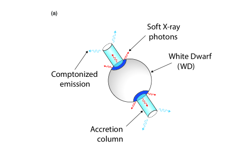
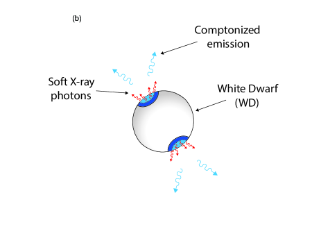
Figure 6: (a) The general scenario of Comptonization in IPs: UV/soft X-ray photons from the star surface (red arrows) are Comptonized by electrons in the optically thick plasma present in the accretion columns. (b) The accretion column is destroyed if the local luminosity on the top of the polar caps is greater than the Eddington. In this case, the UV/soft X-ray photons coming from the star surface are Comptonized by the optically thick plasma (Compton cloud) around to the seed photon emission sites.

The additional soft blackbody component characterized by $<kT_{\mathrm{bb}}>$ of 95 $\pm$ 4 eV, as previously mentioned, is a well known component necessary to account for the soft X-ray emission of some IPs. This component likely corresponds to photons coming from the heated region on the WD surface or photosphere – from the region near to the magnetic pole caps, where the accreting material is dumped, or somewhere else if dense blobs of matter penetrate into the WD photosphere. Part of these soft photons is subject to be Comptonized by the accretion column (the optically thick plasma located nearby to the soft seed photons site).

Interestingly, a good spectral fit was obtained for the PQ Gem and V2400 Oph. These both systems share some characteristics with the polar subclass of mCVs. Namely, PQ Gem is an unusual mCV because it shows a strong soft X-ray component, it is polarized in the optical/infrared (IR) wavebands (Potter et al., 1997), and it has an estimated magnetic field strength $B\sim 8-21\times 10^{6}$ G (Vaeth et al., 1996; Piirola et al., 1993) — which are characteristics of polars. On the other hand, it shows a spin period of 833.4 s (Mason, 1997) and an orbital period of 5.19 h (Hellier et al., 1994) — which are typical of IPs. V2400 Oph is the most polarized IP, leading to the highest magnetic field estimate for any IP ($B\sim 9-27\times 10^{6}$ G), overlapping with the range for low-field polars (Buckley et al., 1995; Vaeth, 1997). In addition, Buckley et al. (1995) showed a strong evidence for a disk-less accretion mechanism in this source. They found that the polarized light varies at 927 s, which was interpreted as the WD spin period. The X-rays are pulsed at 1003 s, corresponding to the beat period between the orbital (3.42 h) and spin cycles. The source does not show any X-ray modulations at the orbital or spin cycles, and the detection of the beat period is expected to be observed in disk-less IPs, showing the signature of pole-flipping accretion (see Joshi et al. (2019) and references therein for a discussion on the nature of the accretion mechanism in this source).

It is worthwhile to emphasize that the presence of an accretion disk is not essential when one uses the Comptonization model. Therefore, we conclude that the good spectral fits of the PQ Gem and IP V2400 Oph spectra is an evidence that the thermal Comptonization may describe the spectral continuum of the polar subclass of mCVs as well.

It is important to stress however that this study is energy band limited, considering only $\sim$ 0.3 – 15 keV XMM-Newton spectra. A future study including broader spectral band (E $>$ 15 keV) may better constrain the range of physical parameters in the Comptonization framework and consequently the spectral indices. Therefore, the analysis of a bigger sample of IP spectra – in different states and WD spin phases – considering data from broadband X-ray missions is highly suitable for a complete characterization and understanding of IPs (and CVs in general) in the Comptonization framework.

5 Summary and Conclusions

We found that the thermal compTT  model can in general successfully fit the continuum of all IPs (13 XMM-Newton Epic-pn observations) in our sample. In this scenario the continuum is produced by seed photons with a mean color temperature $<kT_{\mathrm{s}}>$ of 0.096 $\pm$ 0.013 keV being Comptonized by electrons with a mean plasma temperature $<kT_{\mathrm{e}}>$ 3.05 $\pm$ 0.16 keV located in an optically thick plasma around the central source. In our interpretation, the UV/soft X-ray seed photons are coming from the WD surface (most likely from the region surrounding the magnetic polar caps) and are being Comptonized by hot electrons of (a) the accretion columns or (b) the Compton cloud around the magnetic pole caps of the star. This last case may occurs when accretion columns are not present, namely when $\Gamma\sim 1.3$ and the source has high specific accretion rate.

The spectra of EX Hya, NY Lup, V1223 Sgr and RX J2133.7+5107 show an additional soft X-ray bbody component, with mean temperature $<kT_{bb}>$ of 95 $\pm$ 4 eV, necessary to account for the soft X-ray emission in their spectra. We observed that the presence of this component can strongly depend on both the spectral modelling of the lines in the $\sim$ 0.5 – 1.2 keV soft energy band and the total spectral modeling. This emission likely comes from the star surface, from the heated region surrounding the star magnetic pole caps. Thus, a portion of these photons may be Comptonized by the electrons in the accretion columns or Compton cloud located nearby, surrounding, and on top to the soft seed photon emission regions.

Furthermore, we observed a dichotomy in the spectral shape of IPs, which is driven by the source luminosity and optical depth of the Compton plasma – since $<kT_{\mathrm{s}}>$ and $<kT_{\mathrm{e}}>$ does not change between these two groups of spectra. IPs of high luminosity ($L\sim 10^{32-33}$ erg.s^-1) and $\tau$ ($<\tau>$ of $10.4\pm 4$) show relatively small $\Gamma$ ($<\Gamma>=1.34\pm 0.02$; which indicates the saturated Comptonization in the Compton cloud). Whereas IPs of lower luminosity ($L\sim 10^{31}$ erg.s^-1) and $\tau$ ($<\tau>$ of $6.5\pm 0.4$) show higher $\Gamma$. In this case, $<\Gamma>$ is equal to $1.83\pm 0.19$, which is exactly what is observed in nmCVs. This may indicate closer (intermediate) physical conditions between faint IPs and nmCVs for X-ray emission in the Comptonization framework.

The good spectral fits obtained for the PQ Gem and V2400 Oph sources indicate that thermal Comptonization may also describe the spectral continuum of the polar sub-class of mCVs.

References

- Anzolin et al. (2009) Anzolin, G., de Martino, D., Falanga, M., Mukai, K., Bonnet-Bidaud, J.-M., Mouchet, M., Terada, Y., & Ishida, M. 2009, A&A, 501, 1047
- Arnaud (1996) Arnaud, K. A. 1996, in Astronomical Society of the Pacific Conference Series, Vol. 101, Astronomical Data Analysis Software and Systems V, ed. G. H. Jacoby & J. Barnes, 17
- Barlow et al. (2006) Barlow, E. J., Knigge, C., Bird, A. J., J Dean, A., Clark, D. J., Hill, A. B., Molina, M., & Sguera, V. 2006, MNRAS, 372, 224
- Beardmore et al. (2000) Beardmore, A. P., Osborne, J. P., & Hellier, C. 2000, MNRAS, 315, 307
- Beuermann et al. (2004) Beuermann, K., Harrison, T. E., McArthur, B. E., Benedict, G. F., & Gänsicke, B. T. 2004, A&A, 419, 291
- Bonnet-Bidaud et al. (2006) Bonnet-Bidaud, J. M., Mouchet, M., de Martino, D., Silvotti, R., & Motch, C. 2006, A&A, 445, 1037
- Buckley et al. (1995) Buckley, D. A. H., Sekiguchi, K., Motch, C., O’Donoghue, D., Chen, A.-L., Schwarzenberg-Czerny, A., Pietsch, W., & Harrop-Allin, M. K. 1995, MNRAS, 275, 1028
- Burwitz et al. (1996) Burwitz, V., Reinsch, K., Beuermann, K., & Thomas, H.-C. 1996, A&A, 310, L25
- Cropper et al. (1998) Cropper, M., Ramsay, G., & Wu, K. 1998, MNRAS, 293, 222
- de Martino et al. (2006a) de Martino, D., Bonnet-Bidaud, J.-M., Mouchet, M., Gänsicke, B. T., Haberl, F., & Motch, C. 2006a, A&A, 449, 1151
- de Martino et al. (2004) de Martino, D., Matt, G., Belloni, T., Chiappetti, L., Haberl, F., & Mukai, K. 2004, Nuclear Physics B Proceedings Supplements, 132, 693
- de Martino et al. (2006b) de Martino, D., Matt, G., Mukai, K., Bonnet-Bidaud, J.-M., Burwitz, V., Gänsicke, B. T., Haberl, F., & Mouchet, M. 2006b, A&A, 454, 287
- de Martino et al. (2008) de Martino, D., Matt, G., Mukai, K., Bonnet-Bidaud, J.-M., Falanga, M., Gänsicke, B. T., Haberl, F., Marsh, T. R., Mouchet, M., Littlefair, S. P., & Dhillon, V. 2008, A&A, 481, 149
- Evans & Hellier (2007) Evans, P. A., & Hellier, C. 2007, ApJ, 663, 1277
- Friedjung (1997) Friedjung, M. 1997, New A, 2, 319
- Gotthelf (2003) Gotthelf, E. V. 2003, ApJ, 591, 361
- Haberl & Motch (1995) Haberl, F., & Motch, C. 1995, A&A, 297, L37
- Haberl et al. (2002) Haberl, F., Motch, C., & Zickgraf, F.-J. 2002, A&A, 387, 201
- Hellier (2001) Hellier, C. 2001, Cataclysmic Variable Stars. How and why the vary (Chichester, UK: Srpinger, published with association with Praxis Publising)
- Hellier & Mukai (2004) Hellier, C., & Mukai, K. 2004, MNRAS, 352, 1037
- Hellier et al. (1998) Hellier, C., Mukai, K., & Osborne, J. P. 1998, MNRAS, 297, 526
- Hellier et al. (1994) Hellier, C., Ramseyer, T. F., & Jablonski, F. J. 1994, MNRAS, 271, L25
- HI4PI Collaboration et al. (2016) HI4PI Collaboration, Ben Bekhti, N., Flöer, L., Keller, R., Kerp, J., Lenz, D., Winkel, B., Bailin, J., Calabretta, M. R., Dedes, L., Ford, H. A., Gibson, B. K., Haud, U., Janowiecki, S., Kalberla, P. M. W., Lockman, F. J., McClure-Griffiths, N. M., Murphy, T., Nakanishi, H., Pisano, D. J., & Staveley-Smith, L. 2016, A&A, 594, A116
- Hua & Titarchuk (1995) Hua, X.-M., & Titarchuk, L. 1995, ApJ, 449, 188
- Ishida (1991) Ishida, M. 1991, PhD thesis, , Univ. Tokyo, (1991)
- Ishida et al. (1994) Ishida, M., Mukai, K., & Osborne, J. P. 1994, PASJ, 46, L81
- Ishida et al. (1992) Ishida, M., Sakao, T., Makishima, K., Ohashi, T., Watson, M. G., Norton, A. J., Kawada, M., & Koyama, K. 1992, MNRAS, 254, 647
- Joshi et al. (2019) Joshi, A., Pandey, J. C., & Singh, H. P. 2019, AJ, 158, 11
- Katajainen et al. (2010) Katajainen, S., Butters, O., Norton, A. J., Lehto, H. J., Piirola, V., & Berdyugin, A. 2010, ApJ, 724, 165
- Kuulkers et al. (2006) Kuulkers, E., Norton, A., Schwope, A., & Warner, B. 2006, X-rays from cataclysmic variables, Vol. 39, 421–460
- Landi et al. (2009) Landi, R., Bassani, L., Dean, A. J., Bird, A. J., Fiocchi, M., Bazzano, A., Nousek, J. A., & Osborne, J. P. 2009, MNRAS, 392, 630
- Littlefair et al. (2001) Littlefair, S. P., Dhillon, V. S., & Marsh, T. R. 2001, MNRAS, 327, 669
- Luna et al. (2010) Luna, G. J. M., Raymond, J. C., Brickhouse, N. S., Mauche, C. W., Proga, D., Steeghs, D., & Hoogerwerf, R. 2010, ApJ, 711, 1333
- Maiolino et al. (2020) Maiolino, T., Titarchuk, L., D’Amico, F., Cheng, Z. Q., Wang, W., Orlandini, M., & Frontera, F. 2020, ApJ, 900, 153
- Masetti et al. (2006) Masetti, N., Morelli, L., Palazzi, E., Galaz, G., Bassani, L., Bazzano, A., Bird, A. J., Dean, A. J., Israel, G. L., Landi, R., Malizia, A., Minniti, D., Schiavone, F., Stephen, J. B., Ubertini, P., & Walter, R. 2006, A&A, 459, 21
- Mason (1997) Mason, K. O. 1997, MNRAS, 285, 493
- Mason et al. (1992) Mason, K. O., Watson, M. G., Ponman, T. J., Charles, P. A., Duck, S. R., Hassall, B. J. M., Howell, S. B., Ishida, M., Jones, D. H. P., & Mittaz, J. P. D. 1992, MNRAS, 258, 749
- Mukai et al. (2003) Mukai, K., Kinkhabwala, A., Peterson, J. R., Kahn, S. M., & Paerels, F. 2003, ApJ, 586, L77
- Norton & Watson (1989) Norton, A. J., & Watson, M. G. 1989, MNRAS, 237, 853
- Norton et al. (1991) Norton, A. J., Watson, M. G., & King, A. R. 1991, in Lecture Notes in Physics, Berlin Springer Verlag, Vol. 385, Iron Line Diagnostics in X-ray Sources, ed. A. Treves, G. C. Perola, & L. Stella, 155
- Nwaffiah & Eze (2014) Nwaffiah, J. U., & Eze, R. N. C. 2014, Journal of Korean Astronomical Society, 47, 147
- Oruru & Meintjes (2012) Oruru, B., & Meintjes, P. J. 2012, MNRAS, 421, 1557
- Piirola et al. (1993) Piirola, V., Hakala, P., & Coyne, G. V. 1993, ApJ, 410, L107
- Potter et al. (1997) Potter, S. B., Cropper, M., Mason, K. O., Hough, J. H., & Bailey, J. A. 1997, MNRAS, 285, 82
- Pretorius & Mukai (2014) Pretorius, M. L., & Mukai, K. 2014, MNRAS, 442, 2580
- Snowden et al. (2014) Snowden, S., Valencic, L., Perry, B., Arida, M., & Kuntz, K. D. 2014, The XMM-Newton ABC Guide: An Introduction to XMM-Newton Data Analysis, version 4.5 edn., NASA/GSFC XMM-Newton Guest Observer Facility
- Suleimanov et al. (2016) Suleimanov, V., Doroshenko, V., Ducci, L., Zhukov, G. V., & Werner, K. 2016, A&A, 591, A35
- Sunyaev & Titarchuk (1980) Sunyaev, R. A., & Titarchuk, L. G. 1980, A&A, 86, 121
- Team (2014) Team, X.-N. S. O. 2014, Users Guide to the XMM-Newton Science Analysis System, 10th edn., ESA: XMM-Newton SOC
- Terada et al. (2008) Terada, Y., Hayashi, T., Ishida, M., Mukai, K., Dotani, T., Okada, S., Nakamura, R., Naik, S., Bamba, A., & Makishima, K. 2008, PASJ, 60, 387
- Titarchuk (1994) Titarchuk, L. 1994, ApJ, 434, 570
- Titarchuk et al. (2009) Titarchuk, L., Laurent, P., & Shaposhnikov, N. 2009, ApJ, 700, 1831
- Titarchuk & Lyubarskij (1995) Titarchuk, L., & Lyubarskij, Y. 1995, ApJ, 450, 876
- Vaeth (1997) Vaeth, H. 1997, A&A, 317, 476
- Vaeth et al. (1996) Vaeth, H., Chanmugam, G., & Frank, J. 1996, ApJ, 457, 407
- van Heerden & Meintjes (2015) van Heerden, H., & Meintjes, P. J. 2015, in 3rd Annual Conference on High Energy Astrophysics in Southern Africa (HEASA2015), 5
- Warner (1995) Warner, B. 1995, Cambridge Astrophysics Series, 28
- Wynn et al. (1997) Wynn, G. A., King, A. R., & Horne, K. 1997, MNRAS, 286, 436
- Xu et al. (2016) Xu, X.-j., Wang, Q. D., & Li, X.-D. 2016, ApJ, 818, 136