Hierarchical Regularizers for
Mixed-Frequency Vector Autoregressions

Abstract

Mixed-frequency Vector AutoRegressions (MF-VAR) model the dynamics between variables recorded at different frequencies. However, as the number of series and high-frequency observations per low-frequency period grow, MF-VARs suffer from the “curse of dimensionality”. We curb this curse through a regularizer that permits hierarchical sparsity patterns by prioritizing the inclusion of coefficients according to the recency of the information they contain. Additionally, we investigate the presence of nowcasting relations by sparsely estimating the MF-VAR error covariance matrix. We study predictive Granger causality relations in a MF-VAR for the U.S. economy and construct a coincident indicator of GDP growth. Supplementary Materials for this article are available online.

Keywords: High-dimensionality, Group lasso, Variable selection, Coincident indicators

Introduction

Vector AutoRegressive (VAR) models are a cornerstone for modeling multivariate time series; studying their dynamics and forecasting. However, standard VARs require all component series to enter the model at the same frequency, while in practice macro and financial series are typically recorded at different frequencies; quarterly, monthly, or weekly for instance. One could aggregate high-frequency variables to one common low frequency and continue the analysis with a standard VAR, but such a practice wastes valuable information contained in high-frequency data due to two main reasons. First, high-frequency data are inherently more timely; they closely track the state of the economy in real time. Second, they can help unmask dynamics that would be hidden under temporal aggregation (see e.g., recent discussions in Cimadomo et al., 2021; Paccagnini and Parla, 2021).

Mixed-frequency (MF) models, instead, exploit the information available in series recorded at different frequencies. One commonly used MF models is the MIxed DAta Sampling (MIDAS) regression (Ghysels et al., 2004). While the literature first focused on a single-equation framework for modelling the low-frequency response, the multivariate extension by Ghysels (2016) enabled one to model the relations between high- and low-frequency series in a mixed-frequency VAR (MF-VAR) system. This is known as the stacked MF-VAR approach since the MF-VAR is estimated at the lowest frequency and all higher-frequency variables are treated as separate components series which are stacked in the MF-VAR.

A complication with MF-VARs is that they are severely affected by the “curse of dimensionality”. This curse arises due to two sources. First, the number of parameters grows quadratically with the number of component series, just like for standard VARs. Secondly, specific to MF-VARs, we have many high-frequency observations per low-frequency observation, which each enter as different component series in the model, thereby adding to the dimensionality. Without further adjustments, one would be limited to MF-VARs with few series and/or a small number of high-frequency observations per low-frequency observation.

This curse of dimensionality has mostly been addressed through mixed-frequency factor models (e.g., Marcellino and Schumacher, 2010; Foroni and Marcellino, 2014; Andreou et al., 2019) or Bayesian estimation (e.g., Schorfheide and Song, 2015; Ghysels, 2016; Götz et al., 2016; McCracken et al., 2020; Cimadomo et al., 2021; Paccagnini and Parla, 2021). Sparsity-inducing regularizers form an appealing alternative (see Hastie et al., 2015 for an introduction), but despite their popularity in regression and standard VAR settings (e.g., Hsu et al., 2008; Basu and Michailidis, 2015; Basu et al., 2015; Davis et al., 2016; Callot et al., 2017; Derimer et al., 2018; Smeekes and Wijler, 2018; Barigozzi and Brownlees, 2019; Hecq et al., 2021a), they have only been rarely explored as a tool for dimension reduction in mixed-frequency models. An exception is Babii et al. (2021) who recently used the sparse-group lasso to accommodate the dynamic nature of high-dimensional, mixed-frequency data, thereby providing a complementary structured machine learning perspective to the penalized Bayesian MIDAS approach of Mogliani and Simoni (2021). Nonetheless, they address univariate MIDAS regressions, leaving regularization of MF-VARs unexplored.

Our paper’s first contribution concerns the introduction of a novel convex regularizer that extends the univariate MIDAS approach of Babii et al. (2021) to the multivariate MF-VAR setting. To this end, we propose a mixed-frequency extension of the single-frequency hierarchical regularizer by Nicholson et al. (2020) used for standard VARs that accounts for covariates at different (high-frequency) lags being temporally ordered. We build upon the group lasso with nested groups and encourage a hierarchical sparsity pattern that prioritizes the inclusion of coefficients according to the recency of the information the corresponding series contains about the state of the economy.

In addition to the development of a new MF-VAR with hierarchical lag structure, our paper investigates the presence of nowcasting restrictions in a high-dimensional mixed-frequency setting. According to Eurostat’s glossary, a nowcast is “a rapid [estimate] produced during the current reference period [, say $T^{\ast}$ a particular quarter,] for a hard economic variable of interest observed for the same reference period [$T^{\ast}$]” (Eurostat: Statistics Explained, 2014). In this narrow sense, and contrarily to forecasting, nowcasting makes use of all available information becoming available between (and strictly speaking not including) $T^{\ast}-1$ and $T^{\ast}$. Götz and Hecq (2014) show that nowcasting in (low-dimensional) MF-VARs can be studied through contemporaneous Granger causality tests; by testing the null of a block diagonal error covariance matrix of the MF-VAR. We build on Götz and Hecq (2014) to study nowcasting relations in high-dimensional MF-VARs by sparsely estimating the covariance matrix of the MF-VAR errors. Its sparsity pattern then provides evidence on those high-frequency variables (i.e., the series and their particular time period) one can use to build coincident indicators for the low-frequency main economic indicators.

In a simulation study (Section 4), we find that the hierarchical regularizer performs well in terms of estimation accuracy and variable selection when compared to alternative methods. Furthermore, we accurately retrieve nowcasting relations between the low- and high-frequency variables by sparsely estimating the error covariance matrix. In the application (Section 5), we study a high-dimensional MF-VAR for the U.S. economy. We apply the hierarchical regularizer to characterize the predictive Granger causality relations through a network analysis. Moreover, we investigate which high-frequency series nowcast quarterly U.S. real gross domestic product (GDP) growth, use those to construct a reliable coincident indicator of GDP growth and evaluate its performance pre and post Covid-19.

The remainder of this paper is structured as follows. Section 2 introduces the MF-VAR with hierarchically structured parameters and defines the nowcasting causality relations, Section 3 describes the regularized estimation procedure for MF-VARs and nowcasting causality. Section 4 shows the results on the simulation study, Section 5 on the empirical application of the U.S. economy. Section 6 concludes. Additional results are available in the online appendix.

Mixed-Frequency VARs

We start from Ghysels’ (2016) mixed-frequency VAR systems and include $d$ different high-frequency components. Let $\mathbf{y}(t)$ denote a $k_{L}$-dimensional vector collecting the low-frequency variables for $t=1,\dots,T$. Further, let $\mathbf{x}^{m_{1}}(t)$, $\mathbf{x}^{m_{2}}(t)$,…,$\mathbf{x}^{m_{d}}(t)$ denote the $d$ different, multivariate high-frequency components with $m_{1},\ m_{2},\dots,m_{d}$ number of high-frequency observations per low-frequency period $t$, respectively. Without loss of generality, we take $m_{1}<m_{2}<\dots<m_{d}$. For instance, in a quarter/month/weekly-example $m_{1}=3$ and $m_{2}=12$. Let each component contain $k_{1},k_{2},\dots,k_{d}$ time series of the same high-frequency, respectively. To be precise, each high-frequency component is given by $\mathbf{x}^{m_{i}}(t)=[x_{1}(t,m_{i}),\dots,x_{1}(t,1),\dots,x_{k_{i}}(t,m_{i}),\dots,x_{k_{i}}(t,1)]^{\prime}\in\mathbb{R}^{m_{i}\cdot k_{i}}$ (for $i=1,\dots,d$), where the couple $(t,j)$ indicates higher-frequency period $j=1,\dots,m_{i}$ during the low-frequency period $t$. The MF-VAR${}_{K}(\ell)$ for a lag length of $\ell=1$ is then given by

$$\begin{pmatrix}\mathbf{y}(t)\\ \mathbf{x}^{m_{1}}(t)\\ \vdots\\ \mathbf{x}^{m_{d}}(t)\end{pmatrix}=\mathbf{B}\times\begin{pmatrix}\mathbf{y}(t-1)\\ \mathbf{x}^{m_{1}}(t-1)\\ \vdots\\ \mathbf{x}^{m_{d}}(t-1)\end{pmatrix}+\begin{pmatrix}\mathbf{u}(t)\\ \mathbf{u}^{m_{1}}(t)\\ \vdots\\ \mathbf{u}^{m_{d}}(t)\end{pmatrix},$$ (1)

where $\mathbf{B}\in\mathbb{R}^{K\times K}$ denotes the autoregressive coefficient matrix at lag $1$ for which the total number of series $K$ is given by $K=k_{L}+m_{1}\cdot k_{1}+\dots+m_{d}\cdot k_{d}.$ Further, $\{\mathbf{u}_{t}\in\mathbb{R}^{K}\}_{t=1}^{T}$ is a mean zero error vector with nonsingular contemporaneous covariance matrix $\bm{\Sigma}_{u}$. We focus on stationary time series and assume that all series are mean-centered such that no intercept is included. As for the standard VAR, the $ij^{th}$ entry of $\mathbf{B}$, denoted by $\beta_{ij}$, explains the lagged effect of the $j$th series on the $i$th series. The entries of the autoregressive coefficient matrix thus permits one to study one-step-ahead predictive Granger causality, an often investigated feature also in the context of MF-VARs (e.g., Ghysels et al., 2016; Götz et al., 2016). Besides, given the mixed-frequency nature of the variables, it may be of interest to analyze whether knowing the values of the high-frequency variable at time $t$ helps to predict the low-frequency variable during the same time period and vice versa. This form of hidden, contemporaneous Granger causality between high- and low-frequency variables can be derived from the error covariance matrix $\bm{\Sigma}_{u}$ (see Section 2.2).

We focus on first-order mixed-frequency VARs throughout the paper, extensions to higher-order systems can be easily made, see Remark 2.2. If the true model is multivariate, each component series follows an ARMA$(K\ell,(K-1)\ell)$, see the final equation representation of VARs in Zellner and Palm, 1974, or Cubadda et al., 2009 for a more recent discussion. Besides, a VAR(1) can even yield long-memory processes for $K\rightarrow\infty$ (Chevillon et al., 2018). Hence, as a large system with a small lag length can generate smaller systems with rich and versatile dynamics, it is plausible to assume that the data generating process of a high-dimensional MF-VAR has a small $\ell$. But even a MF-VAR${}_{K}(1)$ model requires one to estimate $K^{2}$ parameters which quickly becomes large since for a fixed $T$ the parameter vector grows (quadratically) with the number of time series included but also due to the high-per-low frequency observations $m_{1},\dots,m_{d}$. In the remainder, we use matrix notation to compactly express the mixed-frequency VAR. To this end, define

$$\bar{\mathbf{y}}_{t} =[\mathbf{y}(t)^{\prime},\mathbf{x}^{m_{1}}(t)^{\prime},\dots,\mathbf{x}^{m_{d}}(t)^{\prime}]^{\prime}\ (K\times 1)\qquad \mathbf{Y} =[\bar{\mathbf{y}}_{1},\dots,\bar{\mathbf{y}}_{N}]^{\prime}\ (N\times K)$$

$$\mathbf{Z} =[\bar{\mathbf{y}}_{0},\dots,\bar{\mathbf{y}}_{N-1}]^{\prime}\ (N\times K)\quad \mathbf{X} =\mathbf{I}_{K}\otimes\mathbf{Z}\ (NK\times K^{2})$$

$$\mathbf{u}_{t} =[\mathbf{u}(t)^{\prime},\mathbf{u}^{m_{1}}(t)^{\prime},\dots,\mathbf{u}^{m_{d}}(t)^{\prime}]^{\prime}\ (K\times 1)\quad \mathbf{U} =[\mathbf{u}_{1},\dots,\mathbf{u}_{N}]^{\prime}\ (N\times K),$$

where $N=T-1$ are the number of time points available given the MF-VAR${}_{K}(1)$, $\mathbf{I}_{K}$ denotes the identity matrix of dimension $K$ and $\otimes$ the Kronecker product. Then the MF-VAR${}_{K}(1)$ can be written as $\mathbf{y}=\mathbf{X}\bm{\beta}+\mathbf{u}$, with $\mathbf{y}=\text{vec}(\mathbf{Y})$, $\bm{\beta}=\text{vec}(\mathbf{B}^{\prime})$, and $\mathbf{u}=\text{vec}(\mathbf{U})$.

In the classical low-dimensional setting $K<N$, the MF-VAR can be estimated by least squares. However, as the number of parameters grows relative to the time series length $T$, least squares becomes unreliable as it results in high variance, overfitting and poor out-of-sample forecasting. We therefore resort to penalization methods. Many authors have used the lasso (Tibshirani, 1996), which attains so called “patternless” sparsity in the parameter matrices of the VAR (e.g., Hsu et al., 2008; Derimer et al., 2018). We, instead, use the dynamic structure of the MF-VAR as a guide in our sparse estimation procedure. Therefore, we propose regularized estimation of MF-VARs that translates information about the hierarchical structure of low- and high-frequency variables into a convex regularizer that delivers structured sparsity patterns appropriate to the context of MF-VARs.

Hierarchical Structures

We describe the hierarchical sparsity patterns that arise in the autoregressive coefficient matrix $\mathbf{B}$ of a MF-VAR. We demonstrate the intuition, for ease of notation, with $k_{L}=k_{1}=\dots=k_{d}=1$, see Remark 2.1 for an extension to multiple series. The parameters of the matrix $\mathbf{B}$ can be divided in $(d+1)^{2}$ different groups as depicted by the sub-matrices in the left panel of Figure 1. We distinguish three types of sub-matrices capturing respectively Own-on-Own, Higher-on-Lower and Lower-on-Higher effects, to extend standard VAR estimation with single-frequencies to mixed-frequencies. The Own-on-Own sub-matrices are $m\times m$ square matrices that lie on the main diagonal and describe the effects of a series’ own lags on itself (with $m_{L}=1$ for the low-frequency variable). The Higher-on-Lower sub-matrices are short, wide $m_{L}\times m_{H}$ matrices, where $L$ and $H$ refer to the corresponding lower- and higher-frequency variable. They lie above the main diagonal and contain the lagged effect of a higher-frequency series onto a series with respective lower frequency. Note that $L$ (and $H$) just identify which of the two variables is of lower (and higher) frequency. Thus, this group does not only contain the effects of the higher-frequency variables onto the variable with the lowest frequency but also describes the interactions between the higher-frequency variables. For instance, in a quarter/month/week-example, these incorporate the effects of the monthly and weekly variable onto the quarterly variable but also the effects of the weekly onto the monthly variable. The Lower-on-Higher sub-matrices are long, thin $m_{H}\times m_{L}$ matrices. They lie below the main diagonal and contain the lagged effect depicting the effect of a lower-frequency series onto a higher-frequency series.

Figure 1: Division of autoregressive coefficient matrix $\mathbf{B}$ into sub-matrices capturing Own-on-Own, Higher-on-Lower and Lower-on-Higher effects.

For each sub-matrix, we impose a hierarchical priority structure for parameter inclusion. Parameters with higher priority within one group should be included in the model before parameters with lower priority within the same group, where the priority value of each parameter depends on how informative a practitioner finds the associated regressor. A priority value of one indicates highest priority for inclusion. More precisely, we introduce a priority value $p_{g}^{ij}\in\{1,\dots,P_{g}\}$ for each element $ij$ belonging to parameter group $g=1,\dots,G$ in the matrix $\mathbf{B}$ to denote its inclusion priority. Here, we order the groups in Figure 1 from left to right and top to bottom. For instance, the top left square is group $g=1$, the rectangle to the right is group $g=2$. If $p_{g}^{ij}<p_{g}^{i^{\prime}j^{\prime}}$ for $i\neq i^{\prime}$ and $j\neq j^{\prime}$, we prioritize parameter $\beta_{ij}$ over $\beta_{i^{\prime}j^{\prime}}$ in the model. The hierarchical structure is imposed for each group $g$ individually and hence in each group the priority values start with value 1 (highest priority) and go up to $P_{g}$ (lowest priority). We do not encode structures where certain parameters of one group should enter the model before certain parameters of another group as our aim is to encode priority of parameter inclusion with respect to the effects of one frequency component (Own/Higher/Lower) on another (Own/Higher/Lower).

These hierarchical priority structures are highly general and could potentially accommodate various structured sparsity patterns in the AR parameter matrix that researchers or practitioners want to encourage. We give special attention to a recency-based priority structure, where the priority value $p_{g}^{ij}$ is set according to the recency of the information the $j$th time series of $\bar{\mathbf{y}}_{t-1}$ contains relative to the $i$th series of $\bar{\mathbf{y}}_{t}$. The more recent the information contained in the lagged predictor, the more informative, and thus the higher its inclusion priority. Figure 2 visualizes the recency-based structure for an example with only one quarterly and one monthly variable having a $4\times 4$ coefficient matrix B and $G=4$ groups. For instance, consider the Higher-on-Lower parameter block, where month three of the previous quarter contains the most recent information, followed by month two and then month one. The priority values are thus increasing from left to right.

Figure 2: Left: Priority values $p^{ij}_{g}$, corresponding to each element $ij$ in the autoregressive coefficient matrix $\mathbf{B}$ for a MF-VAR${}_{4}(1)$. Right: Recency-based penalty structures for parameter groups Own-on-Own, Higher-on-Lower and Lower-on-Higher in a MF-VAR${}_{4}(1)$.

The recency-based priority structure is conceptually similar to other often used restriction schemes in the (MF)-VAR literature. For the Higher-on-Lower group, it is similar to a MIDAS weighting function with decaying shape, for instance an exponential Almon lag polynomial. Both approaches assume a decaying memory pattern in the economic processes, however, in our setting, we do not restrict the parameters to a specific nonlinear function. Besides, our recency-based priorities are similar in spirit to the Minnesota prior in the Bayesian literature (e.g., Cimadomo et al., 2021) in the sense that longer lags are treated differently than shorter lags as they are expected to contain less information about a variable’s current value.

Remark 2.1.

If one were to extend to a MF-VAR${}_{K}(1)$ with multiple time series per frequency component, the total number of groups $G$ becomes $(k_{L}+k_{1}+\dots+k_{d})^{2}$. Then the priority values describing the dependence of the dependent variable having frequency $m_{i}$ on the independent variable having frequency $m_{j}$ would be replicated $k_{i}\times k_{j}$ times. E.g., in a setting with two quarterly and three monthly variables, the priority values describing the effect of monthly series on quarterly series are replicated six times.

Remark 2.2.

If one were to increase the lag length, the total number of groups $G$ would remain unchanged, but each group would additionally incorporate all its higher-order lagged coefficients. Since higher-order lags contain older information, we decrease their priority of inclusion. For example, the Higher-on-Lower group for a MF-VAR${}_{4}(2)$ would have priority values one up to three for lag 1; four up to six for lag 2. We discuss the sensitivity of our empirical results to the maximum lag length in Section 5.3.

Nowcasting Restrictions

The hidden contemporaneous links between high- and low-frequency variables can be investigated in the covariance matrix ${\bm{\Sigma}}_{u}$ of the error terms ${\bf u}_{t}$ in the MF-VAR model (1). Götz and Hecq (2014) test for block diagonality of ${\bm{\Sigma}}_{u}$ to investigate the null of no contemporaneous Granger causality or, to put it differently, the absence of nowcasting relationships between high- and low-frequency indicators. In the remainder, we refer to contemporaneous Granger causality as “nowcasting causality”. The authors show that the conditional single equation model (e.g., MIDAS) with contemporaneous regressors can be misleading as it can change the dynamics observed in a MF-VAR system (e.g., Granger causality relations). We do not face this problem since we work with the reduced form MF-VAR and not with a single equation conditional model derived from the MF-VAR.

In the context of our paper, a detailed inspection of the residual covariance matrix $\widehat{\bm{\Sigma}}_{u}:=\frac{1}{T-\ell}\sum_{t=\ell+1}^{T}\widehat{{\bf u}}_{t}\widehat{{\bf u}}^{\prime}_{t}$ of the high-dimensional MF-VAR is interesting for (at least) two reasons. First, from an economic perspective, we aim to investigate whether there exist high-frequency months, weeks or days of some series that nowcast low-frequency variables. Since this is a correlation measure observed in the symmetric blocks of the residual covariance matrix, we obviously cannot point towards a direction of this contemporaneous link. Lütkepohl (2005, pages 45-48) stresses that the “direction of (nowcasting) causation must be obtained from further knowledge (e.g., economic theory) on the relationship between the variables”. We can only agree on that. Second, from a statistical perspective, we aim to compare the performance of the MF-VAR from Section 2.1 when additional restrictions on the error covariance matrix are considered. Intuitively, this is a Generalized Least Squares (GLS) type improvement over the “unrestricted” hierarchical MF-VAR.

In our economic application (to be discussed in Section 5), we consider quarterly real GDP growth as one of the main low-frequency indicators, and are interested in investigating whether some high-frequency monthly (e.g., retail sales) and/or weekly (e.g., money stock, federal fund rate) series can deliver a coincident indicator of GDP growth with the advantage being that they are released earlier. We do not claim that they directly impact GDP but simply that the business cycle movements detected in those high-frequency variables track the fluctuations of the GDP growth well.

To investigate such nowcasting relations, let us assume a single low-frequency variable and decompose ${\bm{\Sigma}}_{u}$ into four blocks

$${\bm{\Sigma}}_{u}=\left[\begin{array}[]{cc}\sigma_{1.1}^{2}&{\bm{\sigma}}_{.K-1}^{2^{\prime}}\\ {\bm{\sigma}}_{.K-1}^{2}&{\bm{\Sigma}}_{2:K}\end{array}\right],$$

with ${\bm{\Sigma}}_{2:K}$ the $(K-1)\times(K-1)$ block of ${\bm{\Sigma}}_{u}$ corresponding to the covariances between errors of the high-frequency variables. It contains both (co)-variances per high-frequency variable (i.e., its main-diagonal blocks) as well as covariances between different high-frequency variables (i.e., its off-diagonal blocks). $\sigma^{2}_{1.1}$ is the error variance of the low-frequency variables. It is a scalar when there is only one variable but in general it is a square matrix. ${\bm{\sigma}}_{.K-1}^{2}$ is a vector when there is a single low-frequency variable, with the cross-covariances of the errors between low- and high-frequencies. This will be the block we focus on to detect nowcasting relations between each low-frequency variable and each high-frequency variable.

To detect nowcasting relations, we investigate the existence of a sparse matrix

$${\bm{\Sigma}}_{u}^{\ast}=\left[\begin{array}[]{cc}\sigma_{1.1}^{\ast 2}&{\bm{\sigma}}_{.K-1}^{\ast 2^{\prime}}\\ {\bm{\sigma}}_{.K-1}^{\ast 2}&{\bm{\Sigma}}_{2:K}^{\ast}\end{array}\right],$$

where we leave $\sigma_{1.1}^{\ast 2}$ as well as the main-diagonal blocks in ${\bm{\Sigma}}_{2:K}^{\ast}$ unrestricted. The sparsity of the block ${\bm{\sigma}}_{.K-1}^{\ast 2}$ is our main focus as it allows us to detect nowcasting relations between the low-frequency variables and each of the high-frequency ones. The sparsity in the off-diagonal blocks of ${\bm{\Sigma}}_{2:K}^{\ast}$ we allow for is not of main economic interest to our nowcasting application, but it may be of interest in other applications and it does facilitate retrieval of a positive definite ${\bm{\Sigma}}_{u}^{\ast}$ matrix (see Section 3.2).

Remark 2.3.

The case ${\bm{\sigma}}_{.K-1}^{\ast 2}={\bf 0}_{(K-1)\times 1}$ (with one low-frequency variable) corresponds to the block diagonality of ${\bm{\Sigma}}_{u}^{\ast}$ and hence the null of no nowcasting causality.

Remark 2.4.

Unlike for the autoregressive parameter matrix, we do not impose a hierarchical sparsity structure on ${\bm{\sigma}}_{.K-1}^{\ast 2}$ because the middle month could be a better coincident indicator for a quarterly variable than the last month, for instance. Since this is an empirical issue, we prefer to stick to a regularized estimator of the residual covariance matrix that encourages “patternless” sparsity in $\widehat{{\bm{\sigma}}}_{.K-1}^{\ast 2}$.

Finally, to build our coincident indicator, we use a simple procedure which consists of first selecting the variable-period combinations corresponding to non-zero entries in ${\bm{\sigma}}_{.K-1}^{\ast 2}$, standardizing the series and subsequently constructing the first principal component. We rescale the coincident indicator to GDP growth as in Lewis et al. (2021).

Regularized Estimation Procedure of MF-VARs

Hierarchical Group Lasso for Structured MF-VAR

To attain the hierarchical structure presented in Section 2.1, we use a nested group lasso (Zhao et al., 2009) which has been successfully employed for various statistical problems, among which, time series models (e.g., Nicholson et al., 2020), generalized additive models (e.g., Lou et al., 2016), regression models with interactions (e.g., Haris et al., 2016) or banded covariance estimation (e.g., Bien et al., 2016). The group lasso uses the sum of (unsquared) Euclidean norms as penalty term to encourage sparsity on the group-level. Then, either all parameters of a group are set to zero or none. By using nested groups, hierarchical sparsity constraints are imposed where one set of parameters being zero implies that another set is also set to zero. We encourage hierarchical sparsity within each group of parameters by prioritizing parameters with a lower priority value over parameters with a higher one. The proposed hierarchical group estimator for the MF-VAR is given by

$$\widehat{\bm{\beta}} =\underset{\bm{\beta}}{\text{argmin}}\ \Big{\{}\frac{1}{2}\lVert\mathbf{y}-\mathbf{X}\bm{\beta}\rVert_{2}^{2}+\lambda_{\beta}\mathcal{P}_{\text{Hier}}(\bm{\beta})\Big{\}},$$ (2)

where $\mathcal{P}_{\text{Hier}}(\bm{\beta})$ denotes the hierarchical group penalty and $\lambda_{\beta}\geq 0$ is a tuning parameter.

Before introducing the hierarchical group penalty, recall that we distinguish $g=1,\dots,G$ parameter groups in the autoregressive parameter matrix and that $P_{g}$ is the maximum priority value of parameter group $g$. To impose the hierarchical structure within each parameter group $g$, we consider $P_{g}$ nested sub-groups $s_{g}^{(1)},\ldots,s^{(P_{g})}_{g}$. Group $s_{g}^{(1)}$ contains all parameters of group $g$, $s_{g}^{(2)}$ omits those parameters having priority value one, and finally the last sub-group $s_{g}^{(P_{g})}$ only contains those parameters having the highest priority value $P_{g}$. Clearly, a nested structure arises with $s_{g}^{(1)}\supset\dots\supset s_{g}^{(P_{g})}$. Now, denote $\bm{\beta}_{g}^{(p:P_{g})}=[{\bm{\beta}_{g}^{p}}^{\prime},\dots,{\bm{\beta}_{g}^{P_{g}}}^{\prime}]^{\prime}$, for $1\leq p\leq P_{g}$, where $\bm{\beta}_{g}^{p}$ collects the parameters of group $g$ having priority value $p$. We are now ready to define the hierarchical penalty function as

$$\mathcal{P}_{\text{Hier}}(\bm{\beta})=\sum_{g=1}^{G}\sum_{p=1}^{P_{g}}w_{s_{g}^{(p)}}\lVert\bm{\beta}_{g}^{(p:P_{g})}\rVert_{2}.$$ (3)

The hierarchical structure within each group $g$ is built in through the condition that if $\bm{\beta}_{g}^{(p:P_{g})}=\bf{0}$, then $\bm{\beta}_{g}^{(p^{\prime}:P_{g})}=\bf{0}$ where $p<p^{\prime}$.

Remark 3.1.

A related sparse-group lasso penalty has been proposed by Babii et al. (2021). Similar to our penalty, theirs is tailored to the dynamic nature of the mixed-frequency model to account for different high-frequency lags being temporally related. As such, both penalties induce sparsity at two levels: whether a variable is important for explaining another or not; and if important, both steer the effect’s duration via an additional sparsity layer. Via our nested group lasso, we do this by building a hierarchy to cut off the effect of one variable on another after a certain (high-frequency) lag. Via the sparse-group lasso, Babii et al. (2021) regulate the shape of the MIDAS weight function for each group which consists of all high-frequency lags of a single variable.

The weights $w_{s_{g}^{(p)}}$ balance unequally sized nested sub-groups. We take $w_{s_{g}^{(p)}}=\text{card}(s_{g}^{(1)})-\text{card}(s_{g}^{(p)})+1,$ where $\text{card}(\cdot)$ corresponds to the cardinality. As the cardinality of the sub-groups $s_{g}^{(p)}$ is decreasing with $p$, the weights of the nested sub-groups are increasing with $p$. Sub-groups containing parameters with lower priority, i.e., with older information about the state of the economy, are thus penalized more and hence more likely to be zeroed out.

Remark 3.2.

A simple alternative to our proposed weights are equal weights as used in Zhao et al. (2009) or Nicholson et al. (2020), which would lead to less aggressive shrinkage. Simulations in Section 4.1 reveal that the proposed more aggressive weights are preferable for sparsity recognition. In Section 4.4, we include recommendations to guide forecasters in choosing the weights.

Finally, we propose a proximal gradient algorithm (see e.g., Tseng, 2008) to efficiently solve the optimization problem in Equation (2), as detailed in Appendix A.

Regularized Estimation of Nowcasting Causality Relations

To detect nowcasting relations between the low- and high-frequency variables, we use a lasso-penalty to impose “patternless” sparsity on the covariances between low- and high-frequency errors and the covariances between different high-frequency errors (see Section 2.2). The proposed sparse covariance estimator is then given by

$$\widehat{\bm{\Sigma}}^{\ast}_{u}=\underset{\bm{\Sigma}\succ 0}{\text{argmin}}\left\{\frac{1}{2}\left\lVert\widehat{\bm{\Sigma}}_{u}-\bm{\Sigma}\right\rVert_{F}^{2}+\lambda_{\Sigma}\left\lVert\bm{\Sigma^{-}}\right\rVert_{1}\right\},$$ (4)

where $\lambda_{\Sigma}\geq 0$ is a tuning parameter, $\bm{\Sigma}^{-}$ are the elements of the off-diagonal blocks of $\bm{\Sigma}$. Furthermore, for a matrix $\mathbf{A}$, $\lVert\mathbf{A}\rVert_{F}=\lVert\text{vec}(\mathbf{A})\rVert_{F}=(\sum_{ij}\mathbf{A}_{ij}^{2})^{1/2}$ denotes the Frobenius norm and $\lVert\mathbf{A}\rVert_{1}=\lVert\text{vec}(\mathbf{A})\rVert_{1}=\sum_{ij}|\mathbf{A}_{ij}|$ the $l_{1}$-norm.

Remark 3.3.

The mere addition of the $l_{1}$-penalty in problem (4) does not guarantee the estimator $\widehat{\bm{\Sigma}}^{\ast}_{u}$ to be positive definite (see Rothman et al., 2009). To ensure its positive definiteness, the constraint $\bm{\Sigma}\succ 0$ implies that we only consider solutions with strictly positive eigenvalues. Rothman et al. (2009) show that (4) without the constraint $\bm{\Sigma}\succ 0$ essentially boils down to element-wise soft-thresholding of $\bm{\Sigma}^{-}$: the sparse estimate $\widehat{\bm{\Sigma}}^{\ast}_{u}$ is given by $\text{sign}(\bm{\Sigma}^{-})\ \text{max}(|\bm{\Sigma}^{-}|-\lambda_{\Sigma},0).$ If the minimum eigenvalue of the unconstrained solution is greater than 0, then the soft-thresholded matrix is the correct solution to (4). However, if the minimum eigenvalue of the soft-thresholded matrix is below 0, we follow Bien and Tibshirani (2011) and perform the optimization using the alternating direction method of multipliers (Boyd et al., 2011), which is implemented in the R function ProxADMM of the package spcov (Bien and Tibshirani, 2012). Note that similarly to the estimation of the MF-VAR, we solve (4) for a decrementing log-spaced grid of $\lambda_{\Sigma}$-values.

If one wishes to incorporate the estimated nowcasting relations, the autoregressive parameters can be re-estimated by taking the error covariance matrix into account. This results in a type of generalized least squares estimator of $\bm{\beta}$ as given by

$$\widehat{\bm{\beta}}^{\ast}=\underset{\bm{\beta}^{\ast}}{\text{argmin}}\ \Big{\{}\frac{1}{2}\lVert\mathbf{y^{\ast}}-\mathbf{X^{\ast}}\bm{\beta}^{\ast}\rVert_{2}^{2}+\lambda_{\beta^{\ast}}\mathcal{P}_{\text{Hier}}(\bm{\beta}^{\ast})\Big{\}},$$ (5)

where $\mathbf{y^{\ast}}=\widetilde{\bm{\Sigma}}^{-1/2}\mathbf{y}$, $\mathbf{X^{\ast}}=\widetilde{\bm{\Sigma}}^{-1/2}\mathbf{X}$ and $\widetilde{\bm{\Sigma}}=\widehat{\bm{\Sigma}}^{\ast}_{u}\otimes\mathbf{I}_{N}$.

Simulation Study

We assess the performance of the proposed hierarchical group estimator through a simulation study where we compare its performance to three alternatives, namely the ordinary least squares (OLS), the ridge and the lasso.

The set-up of the simulation study is driven by our empirical application (Section 5), namely the small MF-VAR with $K=22$ (one quarterly and seven monthly variables) and $T=125$. The parameter matrix is set to reflect the obtained coefficients which result in a stable MF-VAR. To make a clear distinction between zero and nonzero coefficients, we set all coefficients smaller than 0.01 to zero. As a result, the coefficient matrix does not strictly follow the recency-based hierarchical structure anymore, thereby favoring the hierarchical estimator less compared to its benchmarks. Throughout the paper, we standardized each series to have sample mean zero and variance one as commonly done in the regularization literature before applying a sparse method such that all coefficients have comparable sizes after standardization. To reduce the influence of initial conditions on the data generation process (DGP), we burn in the first 300 observations for each simulation run.

We consider four simulation designs and run $R=500$ simulations in each. The first design compares the estimators in terms of their estimation accuracy and variable selection performance of the autoregressive parameter vector. In the second design, we analyze how well the proposed regularization method can detect the nowcasting relations between the low- and high-frequency variables in $\widehat{\bm{\Sigma}}_{u}^{\ast}$. The third design compares the point forecasts between the hierarchical estimator and its GLS-type version. The fourth design investigates the performance of the proposed estimator for DGPs with varying degree of sparsity.

Autoregressive Estimation Accuracy and Variable Selection

We take the error covariance matrix to be the identity matrix and compare estimation accuracy of the autoregressive parameter vector by calculating the mean squared error

$$\text{MSE}=\frac{1}{R}\sum_{r=1}^{R}\frac{1}{K^{2}}\sum_{k=1}^{K^{2}}(\beta_{k}-\widehat{\beta}_{k}^{(r)})^{2},$$

where $\widehat{\beta}_{k}^{(r)}$ refers to the $k$th element of the estimated parameter vector in simulation run $r$. To investigate variable selection performance, we use the false positive rate (FPR), the false negative rate (FNR) and Matthews correlation coefficient (MCC):

$$\text{FPR}=\frac{1}{R}\sum_{r=1}^{R}\frac{FP}{\#(k:\beta_{k}\neq 0)}\qquad\qquad\text{FNR}=\frac{1}{R}\sum_{r=1}^{R}\frac{FN}{\#(k:\beta_{k}=0)}$$

$$\text{MCC}=\frac{1}{R}\sum_{r=1}^{R}\frac{TP\times TN-FP\times FN}{\sqrt{(TP+FP)(TP+FN)(TN+FP)(TN+FN)}},$$

where $TP$ (and $TN$) are the number of regression coefficients that are estimated as nonzero (zero) and are also truly nonzero (zero) in the model and $FP$ (and $FN$) are the number of regression coefficients that are estimated as zero (nonzero), but are truly nonzero (zero) in the model. Both FPR and FNR should be as small as possible. The MCC balances the two measures and is in essence a correlation coefficient between the true and estimated binary classifications. It returns a value between $-1$ and $+1$ with $+1$ representing a perfect prediction, $0$ no better than random prediction and $-1$ complete discrepancy between prediction and observation. For the regularization methods (i.e., the proposed hierarchical estimator, lasso and ridge), we each time use a grid of 10 tuning parameters and select the one that minimizes the MSE between the estimated and true parameter vector.

Results. We first focus on estimation accuracy, see the left panel in Figure 3. The hierarchical estimator generates the lowest estimation errors. It significantly outperforms all others in terms of MSE as confirmed by paired sample $t$-tests at 5% significance level. OLS suffers as it is an unregularized estimator and thus cannot impose the necessary sparsity on the parameter vector; similarly for ridge which can only perform shrinkage but not variable selection. The hierarchical estimator performs slightly better than lasso in terms of MSE, but the difference is less profound since lasso can also handle sparsity.

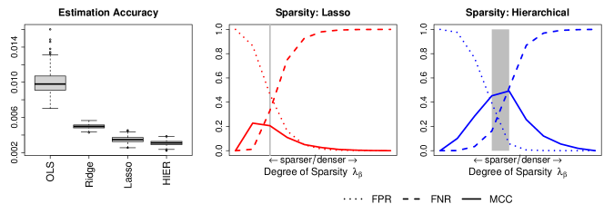
Figure 3: Estimation accuracy for the four estimators (left) and variable selection performance of lasso and the hierarchical estimator (middle and right)

Secondly, we compare the variable selection performance of the lasso and hierarchical estimator, see the middle and right panel of Figure 3, respectively. We plot the average FPR, FNR and MCC for different values of the tuning parameter $\lambda_{\beta}$. The variable selection performance of the hierarchical estimator is in line with its good performance in terms of estimation accuracy. The maximum MCC lies at roughly 0.5, in comparison to the maximum MCC of lasso which only reaches 0.23. The larger FPR of lasso indicates that its estimate is overly sparse, thereby missing important variables in the model. The larger FNR of the hierarchical estimator in comparison to lasso can be explained by the fact that the DGP does not favour the recency-based structure of the hierarchical estimator. Recall that we have set several small coefficients to zero. Thus, it is possible that within one parameter group we have large coefficients with lower priority and zero coefficients with higher priority. Alternatively, we can have hierarchical groups (all coefficients having the same priority) in which some coefficients are zero and some are large. To estimate and capture those important coefficients, our hierarchical estimator estimates some true zero coefficients as nonzero which automatically increases its FNR. Lastly, the grey area in the Figures indicates the 2.5% and 97.5% quantiles of the selected position in the tuning parameter grid across the simulation runs. It illustrates that the maximum MCC lies within the grey area of the hierarchical estimator but does not for lasso.

Finally, we repeat the simulation study using the hierarchical estimator with equal weights; see Figure 8 in Appendix B.1. While the equal weights version generates lower estimation errors, the original weights version performs better in terms of sparsity recognition (MCC). The hierarchical estimator with equal weights shrinks less aggressively, thereby having a higher FNR as many zero coefficients are estimated as small non-zeros.

Nowcasting Relations

We evaluate the detection of the nowcasting relations. To this end, we set the error covariance matrix to the regularized error covariance matrix estimated in the application Section 5.2. Coefficients smaller than 0.03 are set to zero to again ensure a clear distinction between the zeros and non-zeros. We first estimate the model using the four different estimators, calculate the resulting residual covariance matrix and then compute its regularized version through optimization problem (4). In line with our empirical application, we are mainly concerned with the sparsity pattern of the first row/column, namely the one corresponding to the low-frequency variable. Precisely, we investigate its variable selection performance using MCC, FPR and FNR. We estimate the MF-VAR and covariance matrix of the corresponding residuals for a two-dimensional (10 $\lambda_{\beta}$ $\times$ 10 $\lambda_{\Sigma}$) grid of tuning parameters. We select the tuning parameter couple that maximizes the MCC of the regularized covariance matrix in each simulation run. Table 1 contains the results.

Table 1: Variable selection performance (MCC, FPR, FNR) of nowcasting relations in first row/column of the regularized error covariance matrix. “Estimator” refers to the estimator used to estimate the MF-VAR${}_{22}(1)$ and the corresponding residuals from which the covariance matrix is constructed. Standard errors are in parentheses.

Estimator	MCC	FPR	FNR
OLS	0.7111 (0.0052)	0.1937 (0.0058)	0.0960 (0.0064)
Ridge	0.7568 (0.0050)	0.1637 (0.0051)	0.0772 (0.0060)
Lasso	0.7855 (0.0044)	0.1435 (0.0042)	0.0655 (0.0055)
Hierarchical	0.7856 (0.0045)	0.1454 (0.0044)	0.0640 (0.0055)

Results. The performance across estimators is very similar, but the hierarchical estimator and lasso do perform best. Their MCCs lie at roughly 0.78. Their FPRs are slightly higher than their FNR which implies that the nowcasting relations tend to be estimated too sparsely. On the other hand, the low FNR suggests that in general we do not select variables which do not nowcast the low-frequency variable. Lastly, all estimators perform comparably across the tuning parameter grid for $\lambda_{\Sigma}$, but the variability around the selected $\lambda_{\Sigma}$ is higher for OLS and ridge than for lasso and the hierarchical estimator.

Forecast Comparison

We assess whether the best possible forecasting performance of the hierarchical estimator can be improved with its GLS version that incorporates the best nowcasting relations.

The error covariance matrix is set to the same matrix as in Section 4.2. We generate time series of length $T=105$ (as in the forecast of Section 5.3), fit the models to the first $T-1$ observations and use the last observation to compute the one-step-ahead mean squared forecast error for each series. In line with the empirical application, we focus on forecast accuracy of the first series, which represents the low-frequency variable, and select the tuning parameter $\lambda_{\beta}$ that minimizes its squared forecast error. For the selected model, we then estimate its regularized covariance matrix using 10 $\lambda_{\Sigma}$ values and choose the one that maximizes the MCC. Finally, with the selected $\widehat{\bm{\Sigma}}_{u}^{\ast}$, we re-estimate the model according to Equation (5) to compare the forecast performance of the MF-VAR when the additional restrictions on the error covariance matrix are accounted for.

Results. The one-step ahead MSFE for the first series of the hierarchical unrestricted estimator and its GLS version are 0.5508 and 0.5810, respectively. The former significantly outperforms the latter, as confirmed with a paired sample t-test at 1% significance level. The addition of the nowcasting relation may not improve the forecast because the values of the covariances in the covariance matrix of the DGP, particularly of the first row/column, are relatively small in absolute terms. Moreover, it is important to point out that the running time for the estimation of the restricted version is substantially larger than for the unrestricted version. Thus, even if the covariance matrix would be denser, there is a clear trade-off between forecast accuracy and computational efficiency one needs to make.

Varying Degrees of Sparsity

In light of the recent debate on the validity of sparse methods for macroeconomic data (Giannone et al., 2021), we revisit simulation studies 1 and 2 by varying the degree of sparsity of the DGP. Full details on the simulation designs are given in Appendix B.2.

First, we vary the degree of sparsity of the autoregressive parameters in simulation study 1. Figure 9 demonstrates that the MSE of the hierarchical estimator stays relatively constant when the degree of sparsity decreases. Only for the fully dense DGP, we observe a small increase in MSE. The hierarchical estimator with equal weights does not suffer from this. Hence, if one expects a dense DGP or variable selection is not the main priority, the hierarchical estimator with equal weight can be used. On the other hand, if one expects a sparse DGP or seeks parsimonious models to facilitate interpretation, more aggressive shrinkage can be enforced via the hierarchical estimator with proposed weights.

Next, we vary the degree of sparsity in the first row/column of the error covariance matrix of simulation study 2. Here, denser settings do have an effect on the detection of the nowcasting relations. Table 4 shows that the MCC decreases mainly due to an increase in the FPR, meaning that the nowcasting relations are estimated too sparsely.

Macroeconomic Application

We investigate a high-dimensional MF-VAR for the U.S. economy. We use data from 1987 Q3 until 2018 Q4 $(T=126)$ on various aspects of the economy: amongst others output, income, prices and employment, see Table 5 in Appendix C.1 for an overview. The quarterly and monthly series are directly taken from the FRED-QD and FRED-MD datasets which are available at the Federal Reserve Bank of St. Louis FRED database (see McCracken and Ng, 2016, 2020 for more details). The weekly time series are additionally retrieved from the FRED database. The FRED-MD and -QD datasets contain transformation codes to make the data approximately stationary (see column “T-code” in Table 5) which we apply to all series, thereby facilitating replicability and comparison with related research.

To evaluate the influence of additional variables and higher-frequency components, we estimate three MF-VAR models: The small MF-VAR ($K=22$) consists of the quarterly variable at interest, real GDP (GDPC1), and seven monthly variables focusing on (industrial) production, employment and inflation. The medium MF-VAR ($K=55$) contains the small group and eleven additional monthly variables containing further information on different aspects of the economy including financial variables. The large MF-VAR incorporates the variables of the medium group and replaces four monthly variables (CLAIMSx, M2SL, FEDFUNDS, S&P 500) with their equivalent weekly series. See columns “$K=22$”, “$K=55$” and “$K=91$” of Table 5. To ensure that $m_{2}=12$ in the large MF-VAR, we consider all months with more than four weekly observations and disregard the excessive weeks at the beginning of the corresponding month, as in Götz et al. (2016).

We aim to investigate several aspects. First, we focus on the autoregressive parameter estimates of the hierarchical estimator to investigate the predictive Granger causality relations between the series through a network analysis. Second, we concentrate on nowcasting and investigate whether some high-frequency monthly and/or weekly economic series nowcast quarterly U.S. GDP growth and thus can deliver a coincident indicator of GDP growth. Third, we perform a sensitivity analysis of these results. Finally, we perform an out-of-sample expanding window nowcasting exercise including recent data on the Covid-19 pandemic. For ease of the discussion of the results, we follow the variable classification of McCracken and Ng (2016) which can be found in Table 6 in Appendix C.1.

Autoregressive Effects

We first investigate predictive Granger causality relations. To that end, we estimate the MF-VAR using the hierarchical estimator with proposed weights and recency-based priority structure (seasonally adjusted data are used) for all parameter groups and a grid of 10 tuning parameters $\lambda_{\beta}$. The tuning parameter is selected using rolling window time series cross-validation with window size $T_{1}$. For each rolling window whose in-sample period ends at time $t=T_{1},\dots,T-1$, we first standardize each time series to have sample mean zero and variance one using the most recent $T_{1}$ observations, thereby taking possible time variations in the first and second moment of the data into account (see e.g., the Great Moderation Campbell, 2007; Stock and Watson, 2007). Given the evaluation period $[T_{1},T]$, we use the one-step-ahead mean squared forecast error as cross-validation score. $T_{1}=105$, leaving us with 20 observations for tuning parameter selection. We first discuss the results for the small MF-VAR, then summarize the findings for the medium and large MF-VARs.

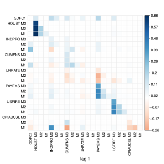
(a)

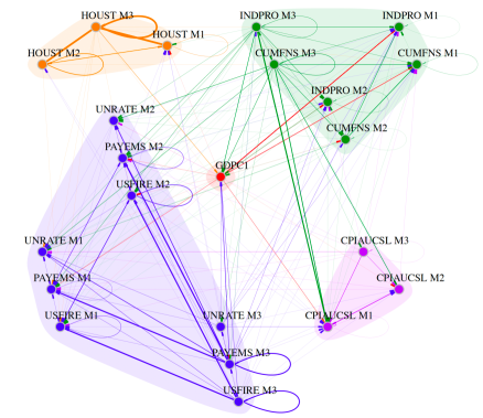
(b)

Figure 4: Small $(K=22)$ MF-VAR: Autoregressive coefficients as a matrix (panel (a)) or as a directed network (panel (b)). The vertices represent the variables, the edges the nonzero coefficients. The edges’ width are proportional to the absolute value of the estimates. Coloring of the vertices and their outgoing edges indicate the macroeconomic categories.

Small MF-VAR. Figure 4(a) depicts the estimated autoregressive coefficient matrix of the hierarchical estimator; 197 of the 484 coefficients (roughly 41%) are estimated as non-zero as indicated by the coloured cells. Figure 4(b) visualizes the same results through a directed network. The vertices represent the variables, the edges the nonzero autoregressive coefficients. The edge’s width is proportional to the absolute value of the estimate. The colors of the vertices and their outgoing edges indicate to which macroeconomic group in McCracken and Ng (2016) the variable and its outgoing effect belong. We summarize the linkages between the macroeconomic categories in Table 2. The columns reflect a macroeconomic category’s out-degree (influence), the rows its in-degree (responsiveness).

Table 2: Small $(K=22)$ MF-VAR: Linkages between macroeconomic group. Entry $(i,j)$ indicates the number of edges from group $j$ to group $i$.

To/From	GDP	Output & Income	Housing	Employment	Prices	In-degree
GDP	0	4	1	3	0	8
Output & Income	4	22	3	16	4	49
Housing	1	1	8	6	0	16
Employment	7	26	5	52	7	97
Prices	2	10	1	9	5	27
Out-degree	14	63	18	86	16	197

We first concentrate on our main variable of interest GDPC1. Eight variables contribute towards its prediction (see first row of Figure 4(a) or incoming edges in panel (b)). Most influential is the macroeconomic group Output & Income as month three and two are included for both variables (INDPRO and CUMFNS). The three variables related to employment (UNRATE, PAYEMS and USFIRE) and HOUST are each selected with their third monthly component. Besides, 14 economic variables are influenced by lagged GDPC1 (see first column of Figure 4(a) or outgoing edges of its vertex in panel (b)). The Employment category has the most incoming edges, nevertheless, the most prominent (thicker) edges indicate that GDPC1 contributes the most to month one of INDPRO and CUMFNS (i.e., the Output & Income group).

Next, we focus on the linkages between macroeconomic groups containing the higher-frequency variables in Table 2. The categories Output & Income and Employment are strongly connected with each other and have the most outgoing edges, even when taking into account that these groups contain more than one monthly variable. Output & Income also contributes to the prediction of Prices and Employment towards Prices as well as Housing. While Prices play a substantial role for Output & Income and Employment, Housing is more relevant for Employment than it is for Output & Income.

Finally, we inspect the linkages within each macroeconomic group (diagonal in Table 2). Employment and Housing display the highest within-group interaction. Zooming in on PAYEMS or USFIRE in Figure 4, we see that their own lagged effects are the strongest, despite them belonging to a group containing more than one high-frequency variable. Within macroeconomic groups, a series’ own lags thus remain the most informative.

When focusing again on the network, we find that the third months of the variables have the most outgoing edges, whereas the first months have the most incoming edges. This is a logical consequence of the recency-based priority structure that we imposed.

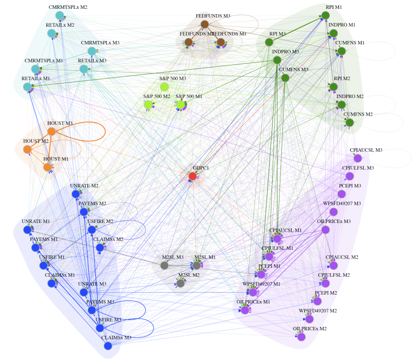
Figure 10: Medium $(K=55)$ MF-VAR: Directed network: the vertices represent the variables, the edges the nonzero coefficients. The edges’ width are proportional to the absolute value of the estimates. Coloring of the vertices and their outgoing edges indicate the macroeconomic categories.

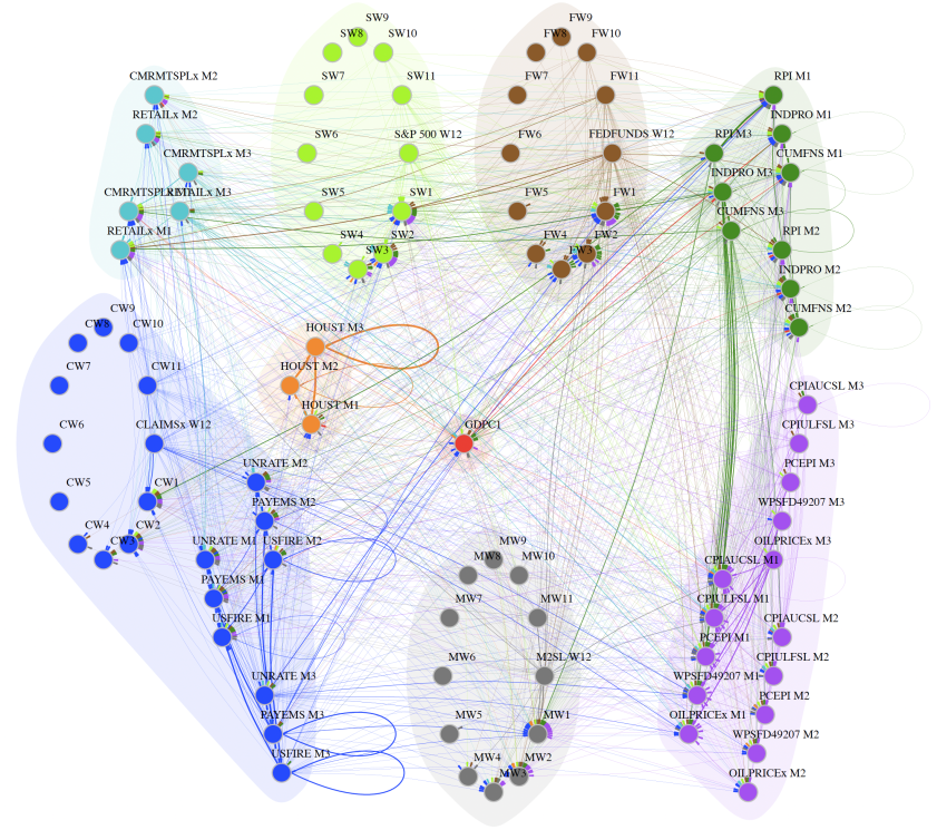
Figure 11: Large $(K=91)$ MF-VAR: Directed network: the vertices represent the variables, the edges the nonzero coefficients. The edges’ width are proportional to the absolute value of the estimates. Coloring of the vertices and their outgoing edges indicate the macroeconomic categories.

Medium and Large MF-VAR. To evaluate the influence of dimensionality, we now compare our results to the two larger MF-VARs. Their networks are given in Figures 10 and 11 in Appendix C.2, whereas Tables 7 and 8 in Appendix C.1 present the linkages between the macroeconomic categories, respectively. The medium MF-VAR has 889 out of 3025 non-zero coefficients (30%), the large MF-VAR 1199 out of 8281 (only 15%). The increase in dimensionality thus induces a higher degree of selectiveness.

Looking at the influencers of GDPC1, we find that the majority of the variables selected for $K=22$ are also selected for the medium and large MF-VAR. In addition, the monetary (M2SL) and financial variables (FEDFUNDS and S&P500) as well as two monthly variables related to sales (CMRMTSPLx and RETAILx) deem to be relevant. Apart from month three of OILSPRICEx and PCEPI in the medium system, no variables related to prices are selected for the prediction of GDP growth. This coincides with the results for the small MF-VAR where CPIAUCSL also only had minor influence. Similarly, the variables that GDPC1 influences in the medium and large system overlap with the selected ones in the small system. Particularly, GDPC1 strongly contributes to the prediction of the variables in the macroeconomic groups Output & Income, illustrated by its thick outgoing edges, and Employment, indicated by the most incoming edges.

Next we focus on the linkages between the macroeconomic groups. For the medium MF-VAR, Table 7 underlines that Output & Income, Sales, Employment and Prices are highly interconnected. Moreover, the group Interest Rates influences the groups Employment and Prices. The latter one is not surprising as FEDFUNDS is usually set to control inflation, hence one can expect changes in the previous quarter to aid in predicting inflation, measured by changes in prices. A similar argument supports the interconnection between Prices and Money. When looking at the diagonal entries of Table 7, we notice that similarly to the small MF-VAR, the groups Employment, Housing and Output & Income have a high within-groups interaction. In contrast to the small system, the within-group linkages among Prices highly increases, which is likely due to the addition of four price variables. The introduction of the weekly variables in the large system does not change the relations among the macroeconomic categories (see Table 8).

Coincident Indicators

We investigate whether some high-frequency monthly and/or weekly economic series nowcast quarterly GDP growth and thus can deliver a coincident indicator. More specifically, we analyze how the performance of the indicator is influenced through (i) the formalization of “sparse” nowcasting relations in the MF-VAR in comparison to a naive approach of constructing a coincident indicator based on the first principal component of all high-frequency variables and (ii) the number of high-frequency components included in the model.

To construct the coincident indicator, we first estimate the MF-VAR using the hierarchical estimator as in Section 5.1. Secondly, we compute the regularized $\widehat{\bm{\Sigma}}_{u}^{\ast}$ from the MF-VAR residuals. We then select the high-frequency variables having a non-zero covariance element in the GDP column and construct the first principal component of the corresponding correlation matrix. We estimate the MF-VAR and corresponding covariance matrix of the MF-VAR residuals for a two-dimensional ($10\times 10$) grid of tuning parameters $\lambda_{\beta}$ and $\lambda_{\Sigma}$. We report the results for the tuning parameter couple that maximizes the correlation between the most parsimonious coincident indicator and GDP growth.

Small MF-VAR. Figure 5(a) plots the U.S. GDP growth against the coincident indicator for the small MF-VAR that maximizes the correlation to a value of 0.7429. The indicator tracks the movements of the GDP growth fairly well. The selected monthly variables from which the first principal component has been constructed are listed on the x-axis of Figure 5(b). Thus, 16 out of the 21 high-frequency variables are selected, since their corresponding covariance with GDP growth is estimated as non-zero. Each variable is included with at least one monthly component. The variables related to Housing (HOUST) and Output & Income (INDPRO and CUMFNS) follow the fluctuations of GDP growth particularly well as all three months are selected. The variables measuring Employment (UNRATE, PAYEMS and USFIRE) have varying levels of contribution. Lastly, the second month of CPIAUCSL, which measures price changes, is also chosen.

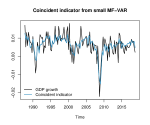
(a)

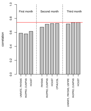
(b)

Figure 5: Small ($K=22$) MF-VAR: Panel (a): U.S. GDP growth versus coincident indicator. Panel (b): Correlation between U.S. GDP growth and different coincident indicators by data release. The horizontal line indicates the correlation with the coincident indicator constructed from all selected nowcasting relations from the entire quarter.

For comparison, a coincident indicator constructed from all high-frequency variables would result in a correlation of 0.7216. Capturing the nowcasting relations in a MF-VAR where the lagged and instantaneous dynamics are separated, thus increases the correlation by 2 percentage points. The advantage of carefully selecting variables before conducting a principal component analysis is a result consistent with Bai and Ng (2008). Furthermore, the correlations with GDP growth are fairly stable across the two-dimensional grid of tuning parameters. In roughly half of the cases, the correlation is at least as high as the one computed from all high-frequency variables. Our findings are thus rather robust to a different choice of selection criterion for the tuning parameters.

GDPC1 is typically released with a relatively long delay (usually one month after the quarter for the first release), whereas the monthly variables are released in blocks at different dates throughout the following month. For instance, the previous month’s UNRATE, PAYEMS and USFIRE are typically released on the first Friday of the following month, whereas the remaining variables are only available around the middle of the month. We follow the release scheme of Giannone et al. (2008) to study the marginal impact of these data releases on the construction of our coincident indicator. We do not take data revisions into account. Hence, our vintages are “pseudo” real-time vintages rather than true real-time vintages.

Figure 5(b) illustrates the achieved correlation between GDP growth and the coincident indicator, updated according to the release dates of the selected variables. As such, the first coincident indicator only uses month one for UNRATE and PAYEMS, whereas the last one is constructed from all selected variables and its correlation with GDP growth is indicated by the horizontal line. The figure shows that intra-quarter information matters. The second month releases have a large impact on the accuracy of the coincident indicator. Particularly, the addition of the variables INDPRO and CUMFNS raises the correlation significantly. In fact, it is possible to construct an almost equally reliable indicator with the data from month one and two compared to one constructed with the data from the entire quarter. Hence, one can build a reliable coincident indicator roughly 1.5 months before the first release of GDP, thereby accounting for the publishing lag of approximately half a month for the monthly series.

Medium and Large MF-VAR. Table 3 summarizes the correlations between GDP growth and the coincident indicators constructed from the different MF-VAR systems. The correlation for the large system (0.7928) is slightly higher than for the medium MF-VAR (0.7715) and both outperform the small system (0.7429).

Table 3: Correlation between U.S. GDP growth and the coincident indicators for the small $(K=22)$, medium $(K=55)$ and large $(K=91)$ MF-VAR groups.

Type of coincident indicator	$K=22$	$K=55$	$K=91$
Nowcasting relations M1	0.6150	0.5128	0.4887
Nowcasting relations M1 + M2	0.7288	0.7495	0.6680
All nowcasting relations	0.7429	0.7715	0.7928
All variables	0.7216	0.7564	0.7557

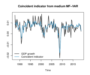
(a)

Variable	Nowcast
RPI	M1	M2	M3
CMRMTSPLx	M1	M2	M3
RETAILx	M1	M2	M3
HOUST	M1	M2	M3
INDPRO	M1	M2	M3
CUMFNS	M1	M2	M3
UNRATE	M1	M2	M3
PAYEMS		M2	M3
USFIRE		M2	M3
CLAIMSx	M1	M2	M3
CPIAUCSL		M2
CPIULFSL		M2	M3
PCEPI		M2
WPSFD49207	M1	M2
OILPRICEx		M2
M2SL	M1		M3
FEDFUNDS		M2	M3
S&P 500	M1	M2	M3

(a)

Figure 12: Medium ($K=55$) MF-VAR: Panel (a): U.S. GDP growth versus coincident indicator. Panel (b): Selected high-frequency variables for the coincident indicator.

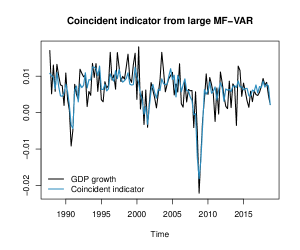
(a)

Variable	Nowcast
RPI	M1	M2	M3
CMRMTSPLx	M1	M2	M3
RETAILx	M1	M2	M3
HOUST	M1	M2	M3
INDPRO	M1	M2	M3
CUMFNS	M1	M2	M3
UNRATE	M1	M2	M3
PAYEMS		M2	M3
USFIRE			M3
CPIAUCSL		M2
CPIULFSL		M2	M3
PCEPI		M2
WPSFD49207	M1	M2
OILPRICEx	M1	M2
CLAIMSx	W1,W2,W3	W6, W7	W10
M2SL	W2, W4	W5, W6, W7	W10, W11
FEDFUNDS	W3, W4	W5, W7, W8	W9, W11
S&P 500	W2, W4	W6, W8,	W9, W10, W11, W12

(a)

Figure 13: Large ($K=91$) MF-VAR: Panel (a): U.S. GDP growth versus coincident indicator. Panel (b): Selected high-frequency variables for the coincident indicator.

Full details on the medium and large MF-VAR are available in Appendix C.2: Figures 12(a) and 13(a) show that both indicators behave similarly and can better pick up the drop in GDP growth during the financial crisis than the coincident indicator of the small system. Many of the variables selected for the coincident indicator of the small MF-VAR are also selected for the two larger MF-VARs (see Figures 12(b) and 13(b)): There is a clear focus on variables related to (industrial) output, sales and employment whereas variables measuring price changes have a smaller influence. For the large MF-VAR 28 weekly variables are selected, thereby making it valuable to incorporate higher-frequency variables. But the mere addition of variables does not lead to a larger correlation, emphasizing that selection is important: Table 3 illustrates that the advantage of selecting the nowcasting relations in the MF-VARs persists as the correlation achieved from the first principal component with all variables is lower. Lastly, the coincident indicator constructed from the selected variables from month one and two for the medium system performs comparable to the one constructed from all selected variables, in line with our finding for the small MF-VAR.

Sensitivity Analyses

We investigate the sensitivity of our results regarding (i) the choice of weights for the hierarchical estimator, (ii) the maximal lag length of the MF-VAR, (iii) the inclusion of daily high-frequency data, and (iv) forecast comparisons.

Equal Weights. We use the hierarchical estimator with equal weights and present the autoregressive linkages between the macroeconomic groups for the MF-VARs in Tables 9-11 of Appendix C.3. Using equal weights corresponds to weaker penalization, hence the networks become denser, but the main conclusions regarding the inter-dependencies remain unchanged. Next, we revisit the results on the coincident indicators in Table 12. For the small MF-VAR, the results are identical. For the medium and the large MF-VAR, respectively more and fewer high-frequency variables are selected for the coincident indicator which only affects its correlation with GDP growth in the first two months.

Lag Length. We re-estimate the small MF-VAR with the hierarchical estimator using a maximal lag $\ell=1,2,$ or $4$. Practically all coefficients from the second lag onwards (more than 98%) are zeroed out, and more first-order coefficients are shrunken towards zero. Both the Bayesian and Akaike Information Criterion indicate one to be the “optimal” lag length.

Daily Data. To investigate the behavior of the hierarchical estimator in presence of daily high-frequency components, we replace the weekly financial variables (FEDFUNDS, S&P500) in the large MF-VAR with 60 daily component series for each. This leads to an “ultra-large” MF-VAR with $K=187$ component series instead of the large MF-VAR with $K=91$ series. Results are detailed in Appendix C.4. Only 5% of the autoregressive coefficients are estimated as non-zero, supporting our previous finding that an increase in dimensionality induces a higher degree of selectiveness. The influencers of GDPC1 stay roughly the same as in large MF-VAR. Interest Rate and Stock Price are selected with only two and three components respectively. The coincident indicator benefits from the usage of the more timely daily instead of weekly financial data only in the beginning of the quarter (for the first two months), but not when using the daily data from the whole quarter.

Forecast Comparison. We investigate the out-of-sample forecast performance of the hierarchical estimator, as detailed in Appendix C.5. We compare its performance to the random walk (RW) and AR(1) model as two popular, simple univariate benchmarks; a traditional quarterly VAR(1), estimated by OLS, with all higher-frequency variables aggregated to the quarterly level; and the three alternative estimators from Section 4 (OLS, ridge and lasso). Table 15 provides the one-step ahead MSFE for GDPC1 across all MF-VARs.

The hierarchical estimator generally outperforms the AR, RW, quarterly VAR and MF-VAR OLS, thereby indicating that higher-frequency variables as well as variable selection help to predict GDP growth. The large MF-VAR with hierarchical estimator attains the lowest MSFE. Both the hierarchical estimator and lasso are included in the Model Confidence Set (Hansen et al., 2011) for two out of the three MF-VARs. The quarterly VAR is not included; information contained in high-frequency series is thus beneficial in our application for forecasting GDP growth.

Nowcasting GDP growth pre and post Covid-19

The Covid-19 pandemic has caused a dramatic drop in economic activity worldwide including the U.S. We end by assessing the performance of our coincident indicators in an out-of-sample expanding window nowcasting exercise with evaluation period 2019 Q1 until 2021 Q2, thereby covering the recent pandemic. For each current quarter in the expanding window approach, we estimate the MF-VAR with the hierarchical estimator (using data until the previous quarter), select the high-frequency variables for the coincident indicator from the residual covariance matrix as in Section 5.2 and obtain their loadings on the first principal component. The nowcasts are then calculated by multiplying these loadings with the out-of-sample high-frequency data of the current quarter.

	$K=22$	$K=55$	$K=91$
Nowcasting	0.1587	0.1385	0.1782
relations M1
Nowcasting	0.0661	0.0340	0.0431
relations M1 + M2
All nowcasting	0.0337	0.0875	0.0919
relations

(a)

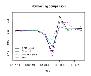
(a)

Figure 6: Panel (a): Nowcasting performance (mean squared nowcast errors of GDP growth, multiplied by 100) of the three MF-VARs for 2019 Q1 to 2021 Q2. Panel (b): U.S. GDP growth versus our coincident indicator (CI), and the B-BVAR and SPF nowcasts.

The mean squared nowcast errors between GDP growth and the coincident indicators constructed from the three MF-VARs are depicted on the last line of the table in Figure 6(a). The coincident indicator of the small MF-VAR attains the best accuracy, the error more than doubles for the larger MF-VARs. In addition, we track the nowcasting accuracy as the quarter progresses, thereby constructing the coincident indicator only from the selected high-frequency variables from the first month (first line), or the first two months (second line in the table). For the best performing small MF-VAR, the nowcasts gradually improve as new data gets released along the quarter, with the largest improvement occurring when adding high-frequency data from the second month to the first.

Next, we discuss the stability through time of the selected variables from which the coincident indicator of the small MF-VAR has been constructed. Panel(a) of Figure 7 shows the selected high-frequency variables for each end point of the expanding window. Panel(b) summarizes them according to the macroeconomic group they belong to. Before the pandemic hits the U.S. economy in 2020 Q1, the selection of the high-frequency variables was very stable. Almost all variables are selected with all monthly components, the exceptions are UNRATE, USFIRE and CPIAUCSL. At the onset of the pandemic, a clear break in variable selection occurs: the coincident indicator is much more sparsely constructed thereby only using data on the Output & Income group from the first month.

Figure 7: Small ($K=22$) MF-VAR: Panel(a): Selected high-frequency variables for the coincident indicator. Panel(b): Fraction of non-zero coefficients in each macroeconomic category to the total number of non-zero coefficients in the coincident indicator. The horizontal axis represents the ending date of each expanding window.

Finally, we compare the performance of the coincident indicator of the small MF-VAR with two state-of-the-art benchmarks, one Bayesian and one survey. We use the “blocking” Bayesian MF-VAR (B-BVAR) by Cimadomo et al. (2021) since it also relies on the stacked MF-VAR approach. Second, we use the GDP nowcasts of the Survey of Professional Forecasters (SPF). Figure 6(b) plots GDP growth against the three different nowcasts for 2019 Q1 to 2020 Q2. Overall, all methods track the same fluctuations in the business cycle. Before the pandemic, all nowcasts are practically the same and very close to actual GDP growth. When the pandemic hits the economy, some differences can be observed. First, the SPF does not pick up the slight drop in GDP growth in Q1 2020. This can be explained by the fact that the SPF nowcasts are released during the second month of a quarter, while most countries only went into lockdown by March. Second, the drop in economic activity in 2020 Q2 is very pronounced for the SPF, much less so for our coincident indicator and the B-BVAR nowcast. The recovery in Q3 thereafter is best tracked by the B-BVAR. Our coincident indicator and the B-BVAR nowcasts align again from Q4 onwards.

Conclusion

We introduce a convex regularization method tailored towards the hierarchically ordered structure of mixed-frequency VARs. To this end, we use a group lasso with nested groups which permits various forms of hierarchical sparsity patterns that allows one to discriminate between recent and obsolete information. Our simulation study shows that the proposed regularizer can improve estimation and variable selection performance. Furthermore, nowcasting relations can be detected from the sparsity pattern of the covariance matrix of the MF-VAR errors. Those high-frequency variables that nowcast the low-frequency variables, as evident from their non-zero contemporaneous link, can deliver a coincident indicator of the low-frequency variable. Constructing coincident indicators from a group of selected variables rather than all permits policy makers to get an earlier grasp of the state of the economy, as can be seen from our economic application on U.S. GDP growth.

The proposed MF-VAR method is quite flexible and can be extended in various ways. First, regularization via restrictions other than sparsity can be explored. Temporal aggregation restrictions, for instance, can be imposed in the MF-VAR by exploiting fusion penalties (e.g., Yan and Bien, 2021) that encourage similarity across certain coefficients. For monthly stock data it could, for instance, be interesting to encourage the effects of all months on the quarterly variable to be similar, thereby implicitly aggregating the monthly variable to the quarterly level. Second, an interesting path for future research concerns the extension of our method to enable structural analysis as recently done in a Bayesian set-up by e.g., Cimadomo et al. (2021) who use generalized impulse responses to track transmission mechanisms of low-frequency shocks hitting the U.S. economy, or Paccagnini and Parla (2021) who use orthogonalized impulse responses to identify the impact of high-frequency shocks thereby revealing a temporal aggregation bias when adopting single low-frequency models instead of mixed-frequency ones. Lastly, while we consider MF-VAR for stationary data, a natural next step would be to allow for non-stationarity by building on the lag-augmentation idea of Toda and Yamamoto (1995) as done in Götz and Hecq (2019) for low-dimensional mixed MF-VARs or Hecq et al. (2021b) for high-dimensional VARs.

Supplemental Materials

R-code:

Supplemental files for this article include R-code to reproduce all results. Please consult the file README in the zip file for more details. (Code.zip, zip archive)

Appendix:

The Appendix contains implementation details on the algorithm, and additional results on the simulations and empirical application. (Appendix.pdf)

Appendix A Algorithm

Algorithm 1 provides an overview of the proximal gradient algorithm (see e.g., Tseng, 2008) to efficiently solve the optimization problem in Equation (2). A key ingredient of the algorithm concerns the proximal operator $\text{Prox}_{v\lambda\mathcal{P}(\cdot)}$ which has a closed-form solution making it extremely efficient to compute. Indeed, the updates of each hierarchical group $p=1,\dots,P_{g}$ correspond to a groupwise soft thresholding operation given by $\text{max}(1-v\lambda\cdot w_{s_{g}^{(p)}}/\lVert\widetilde{\bm{\beta}}_{s_{g}^{(p)}}\rVert_{2},0)\ \widetilde{\bm{\beta}}_{s_{g}^{(p)}}$ with $v$ being the step size which we set equal to the largest singular value of $\mathbf{X}$. Algorithm 1 requires a starting value $\bm{\beta}[0]$ which we initially set equal to $\bf{0}$. Finally, while the algorithm is given for a fixed value of the tuning parameter $\lambda$, it is standard in the regularization literature to implement it for a decrementing log-spaced grid of $\lambda$ values. The starting value $\lambda_{\text{max}}$ is an estimate of the smallest value that sets all coefficients equal to zero. For each smaller $\lambda$ along the grid, we use the outcome of the previous run as a warm-start for $\bm{\beta}[0]$.

Algorithm 1 Accelerated proximal gradient method

0:  $\mathbf{y}$, $\mathbf{X}$, $\mathcal{P}(\bm{\beta})$, $\lambda$, $\varepsilon$ initialization:

• $\bm{\beta}[1]\leftarrow\bm{\beta}[2]\leftarrow\bm{\beta}[0]$

• step size $v$ which is set equal to the largest singular value of $\mathbf{X}$

  for $r=3,4,...$ do

     for $g=1,...,G$ do

        $\ddot{\bm{\beta}}_{g}\leftarrow\bm{\beta}_{g}[r-1]+\frac{r-2}{r+1}\Big{(}\bm{\beta}_{g}[r-1]-\bm{\beta}_{g}[r-2]\Big{)}$

        $\bm{\beta}_{g}[r]\leftarrow\text{Prox}_{v\lambda\mathcal{P}(\cdot)}\Big{(}\ddot{\bm{\beta}}_{g}-v\nabla_{\bm{\beta}_{g}}\mathcal{L}(\ddot{\bm{\beta}}_{g})\Big{)}$

        where $\nabla_{\bm{\beta}_{g}}\mathcal{L}(\ddot{\bm{\beta}}_{g})=-(\mathbf{y}-\mathbf{X}_{\bm{\beta}_{g}}\ddot{\bm{\beta}}_{g}-\mathbf{X}_{\bm{\beta}_{f>g}}\bm{\beta}_{f>g}[r-1]-\mathbf{X}_{\bm{\beta}_{f<g}}\bm{\beta}_{f<g}[r])^{\prime}\mathbf{X}_{\bm{\beta}_{g}}$

     end for

     if $\lVert\bm{\beta}[r]-\bm{\beta}[r-1]\rVert_{\infty}\leq\varepsilon$ then

        break

     end if

  end for

  return  $\bm{\beta}[r]$

Appendix B Simulation Study

Sensitivity Analysis: Choice of weights for hierarchical estimator

Figure 8 compares the results of simulation study 1 for the hierarchical estimator with the proposed weights $w_{s_{g}^{(p)}}=\text{card}(s_{g}^{(1)})-\text{card}(s_{g}^{(p)})+1$ and equal weights.

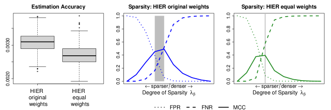
Figure 8: Estimation accuracy for the hierarchical estimator with original and equal weights (left) and variable selection performance with original (middle) and equal weights (right).

Sensitivity Analysis: Denser DGPs

To assess the effect on the hierarchical estimator of varying degrees of sparsity in the autoregressive parameters and the covariance matrix of the error terms, we repeat simulation study 1 and simulation study 2 with varying degrees of sparsity in their respective DGPs.

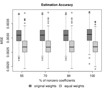
Figure 9: Estimation accuracy for the hierarchical estimator with original (dark grey) and equal weights (light grey) across DGPs with varying degrees of sparsity in the AR coefficients.

For simulation study 1, we gradually increase the percentage of non-zero coefficients in the autoregressive parameters across four settings. The sparsest setting (55% of non-zero coefficients) starts from the design used in Section 4.1 where all coefficients smaller than 0.01 are set to zero. For the second setting (70% non-zeros), all coefficients smaller than 0.002 are set to zero. For the third setting (84% non-zeros), we take the unaltered parameter matrix from Section 4.1. For the densest setting (100% non-zeros) all zero coefficients of the sparsest setting are assigned a value of 0.01. Figure 9 gives the results.

For simulation study 2, we gradually increase the percentage of non-zero coefficients in the first row/column of the error covariance matrix across four settings. The sparsest setting corresponds to the design of Section 4.2 with 62% non-zeros. We then increase the density towards respectively 76%, 90% and 100% non-zeros by each time setting the remaining zero coefficients in the first row/column to 0.03. Table 4 displays the results.

Table 4: Variable selection performance (MCC, FPR, FNR) of nowcasting relations for varying degrees of sparsity in first row/column of the regularized error covariance matrix. Standard errors are in parentheses.

	% of non-zero coefficients in first row/column
	62	76	90	100
MCC	0.7792 (0.0044)	0.7037 (0.0046)	0.5427 (0.0093)	NA1
FPR	0.1448 (0.0045)	0.1301 (0.0057)	0.2040 (0.0066)	0.2352 (0.0081)2
FNR	0.0735 (0.0059)	0.1488 (0.0059)	0.0400 (0.0067)	NA1

• FNR and MCC are not defined since number of TN is zero.

• Tuning parameter selection based on maximizing the correlation between the most parsimonious coincident indicator and the first series since the MCC is not available.

Appendix C Macroeconomic Application

Additional Tables

Table 5: Data description table. Column T-code denotes the data transformation applied to a time-series, which are: (1) not transformed, (2) $\Delta x_{t}$, (3) $\Delta^{2}x_{t}$, (4) $\text{log}(x_{t})$, (5) $\Delta\text{log}(x_{t})$, (6) $\Delta^{2}\text{log}(x_{t})$. Columns $K=22$, $K=55$ and $K=91$ indicate whether and at which frequency the variable was included in the model.

FRED Code	Description	T-code	$K=22$	$K=55$	$K=91$
GDPC1	Real Gross Domestic Product	5	Q	Q	Q
RPI	Real Personal Income	5		M	M
CMRMTSPLx	Real Manufacturing and	5		M	M
	Trade Industries Sales
RETAILx	Retail and Food Services Sales	5		M	M
HOUST	Housing Starts: Total	4	M	M	M
INDPRO	IP Index	5	M	M	M
CUMFNS	Capacity Utilization: Manufacturing	2	M	M	M
UNRATE	Civilian Unemployment Rate	2	M	M	M
PAYEMS	All Employees: Total nonfarm	5	M	M	M
USFIRE	All Employees: Financial Activities	5	M	M	M
CLAIMSx	Initial Claims	5		M	W
CPIAUCSL	CPI : All Items	6	M	M	M
CPIULFSL	CPI : All Items Less Food	6		M	M
PCEPI	Personal Cons. Expend.: Chain Index	6		M	M
WPSFD49207	PPI: Finished Goods	6		M	M
OILPRICEx	Crude Oil	6		M	M
M2SL	M2 Money Stock	6		M	W
FEDFUNDS	Effective Federal Funds Rate	2		M	W
S&P 500	S&P’s Stock Price Index	5		M	W

Table 6: Categories of monthly series in the medium ($K=55$) MF-VAR group, following the grouping of McCracken and Ng (2016) in their Appendix.

Macroeconomic category	FRED Code
Output & Income	RPI, INDPRO, CUMFNS
Sales	CMRMTSPLx, RETAILx
Housing	HOUST
Employment	UNRATE, PAYEMS, USFIRE, CLAIMSx
Prices	CPIAUCSL, CPIULFSL, PCEPI, WPSFD49207
	OILPRICEx
Money	M2SL
Interest rates	FEDFUNDS
Stock prices	S&P 500

Table 7: Medium $(K=55)$ MF-VAR: Linkages between macroeconomic group. Entry $(i,j)$ indicates the number of edges from group $j$ to group $i$.

To / From	GDP	Output	Sales	Housing	Employ-	Prices	Money	Interest	Stock	In-
		& Income			ment			Rate	Prices	degree
GDP	0	3	2	1	4	2	2	0	1	15
Output & Income	5	36	18	2	30	27	8	9	15	150
Sales	4	19	11	5	30	28	6	6	6	115
Housing	1	1	2	8	6	0	1	0	0	19
Employment	9	36	21	8	70	29	11	14	10	208
Prices	8	45	24	5	45	72	10	15	15	239
Money	1	10	4	1	10	12	6	3	3	50
Interest Rate	1	6	8	2	14	9	2	6	5	53
Stock Prices	1	8	4	1	6	13	2	2	3	40
Out-degree	30	164	94	33	215	192	48	55	58	889

Table 8: Large $(K=91)$ MF-VAR: Linkages between macroeconomic group. Entry $(i,j)$ indicates the number of edges from group $j$ to group $i$. Weekly variables are separated.

To / From	GDP	Output	Sales	Housing	Employ-	Prices	CLAIMSx	Money	Interest	Stock	In-
		& Income			ment				Rate	Prices	degree
GDP	0	4	2	1	4	1	1	2	2	2	19
Output & Income	7	35	20	4	23	26	13	18	18	16	180
Sales	4	20	11	4	23	24	10	11	12	11	130
Housing	1	1	2	8	6	0	0	1	1	1	21
Employment	6	31	21	5	52	16	10	11	14	8	174
Prices	8	47	26	5	28	71	24	17	24	27	277
CLAIMSx	2	16	9	4	9	14	9	8	10	5	86
Money	2	18	11	4	16	25	7	11	10	8	112
Interest Rate	2	20	9	3	16	13	7	9	13	7	99
Stock Prices	2	15	11	6	13	25	5	9	7	8	101
Out-degree	34	207	122	44	190	215	86	97	111	93	1199

Additional Figures

Sensitivity analysis: Hierarchical estimator with equal weights

Table 10: Small $(K=22)$ MF-VAR with equal weights: Linkages between macroeconomic group. Entry $(i,j)$ indicates the number of edges from group $j$ to group $i$.

To/From	GDP	Output & Income	Housing	Employment	Prices	In-degree
GDP	0	4	1	5	0	10
Output & Income	4	32	6	24	16	82
Housing	1	2	9	9	0	21
Employment	5	37	6	68	11	127
Prices	3	16	1	17	9	46
Out-degree	13	91	23	123	36	286

Table 11: Medium $(K=55)$ MF-VAR with equal weights: Linkages between macroeconomic group. Entry $(i,j)$ indicates the number of edges from group $j$ to group $i$.

To / From	GDP	Output	Sales	Housing	Employ-	Prices	Money	Interest	Stock	In-
		& Income			ment			Rate	Prices	degree
GDP	0	3	3	1	5	1	2	1	2	18
Output & Income	4	68	31	7	60	55	17	20	19	281
Sales	4	36	24	7	59	55	14	15	16	230
Housing	1	1	2	9	8	0	1	0	0	22
Employment	5	48	44	10	107	53	23	22	21	333
Prices	10	101	55	6	87	155	17	30	31	492
Money	1	17	7	3	22	18	8	6	3	85
Interest Rate	0	3	11	1	16	21	1	9	7	69
Stock Prices	0	19	8	5	11	26	8	9	9	95
Out-degree	25	296	185	49	375	384	91	112	108	1625

Table 12: Large $(K=91)$ MF-VAR with equal weights: Linkages between macroeconomic group. Entry $(i,j)$ indicates the number of edges from group $j$ to group $i$. Weekly variables are separated.

To / From	GDP	Output	Sales	Housing	Employ-	Prices	CLAIMSx	Money	Interest	Stock	In-
		& Income			ment				Rate	Prices	degree
GDP	0	4	4	1	5	1	2	5	5	3	30
Output & Income	6	68	35	7	45	56	49	62	52	57	437
Sales	5	32	24	8	42	51	32	37	38	39	308
Housing	1	1	2	9	8	0	0	0	2	1	24
Employment	4	35	33	4	69	26	35	27	38	28	299
Prices	10	101	50	22	57	152	93	72	78	104	739
CLAIMSx	2	60	41	13	35	49	123	110	116	87	636
Money	2	63	29	22	45	71	103	140	123	94	692
Interest Rate	3	74	28	3	52	54	84	115	135	105	653
Stock Prices	3	52	33	18	48	79	59	111	106	121	630
Out-degree	36	490	279	107	406	539	580	679	693	639	4448

Table 13: Correlation between U.S. GDP growth and the coincident indicators for the small $(K=22)$, medium $(K=55)$ and large $(K=91)$ MF-VAR groups with equal weights.

Type of coincident indicator	$K=22$	$K=55$	$K=91$
Nowcasting relations M1	0.6150	0.2658	0.5528
Nowcasting relations M1 + M2	0.7288	0.7780	0.7769
All nowcasting relations	0.7429	0.7705	0.7956
All variables	0.7216	0.7564	0.7557

Sensitivity analysis: Daily data

Table 14: Ultra-large $(K=187)$ MF-VAR: Linkages between macroeconomic group. Entry $(i,j)$ indicates the number of edges from group $j$ to group $i$. Weekly and daily variables are separated.

To / From	GDP	Output	Sales	Housing	Employ-	Prices	CLAIMSx	Money	Interest	Stock	In-
		& Income			ment				Rate	Prices	degree
GDP	0	5	3	1	4	2	2	2	2	3	24
Output & Income	6	42	23	5	27	30	14	18	26	29	220
Sales	5	21	16	4	24	26	11	12	17	18	154
Housing	1	0	2	8	6	0	0	0	2	6	25
Employment	7	31	22	5	53	19	10	8	22	25	202
Prices	7	58	29	8	34	89	25	20	38	44	352
CLAIMSx	3	16	10	5	12	21	9	8	16	14	114
Money	2	19	12	4	18	24	9	14	14	15	131
Interest Rate	3	25	18	6	24	29	13	17	40	22	197
Stock Prices	5	29	19	9	30	43	10	16	27	38	226
Out-degree	39	246	154	55	232	283	103	115	204	214	1645

Table 15: Correlation between U.S. GDP growth and the coincident indicators for the large $(K=91)$ and ultra-large ($K=187$) MF-VAR.

Type of coincident indicator	$K=91$	$K=187$
Nowcasting relations M1	0.4887	0.6617
Nowcasting relations M1 + M2	0.6680	0.7303
All nowcasting relations	0.7928	0.7893
All variables	0.7557	0.7337

Sensitivity analysis: Forecast Comparison

We use a rolling-window set-up with window size $T_{1}=105$, providing us 20 quarterly observations for forecast comparison. For each rolling window, we select the value of $\lambda_{\beta}$ that minimizes the one-step-ahead squared forecast error for our main variable of interest GDPC1. The MSFE for GDPC1 for the unrestricted hierarchical estimator across all MF-VARs is given in Table 16.

Table 16: Rolling out-of-sample one-step-ahead MSFE of GDPC1. Forecast methods in the 75% Model Confidence Set (MCS) are in bold. Standard errors are in parentheses.

Estimator	Univariate	Multivariate
		$K=22$	$K=55$	$K=91$
AR	0.4137 (0.1880)
RW	0.6969 (0.3636)
Quarterly VAR		0.3070 (0.0907)	0.3624 (0.1094)
OLS		0.5884 (0.1977)	0.9285 (0.2572)	2.6267 (0.9511)
Ridge		0.2307 (0.0977)	0.2191 (0.0761)	0.1630 (0.0491)
Lasso		0.1674 (0.0886)	0.1565 (0.0773)	0.1326 (0.0666)
Hierarchical		0.1678 (0.0824)	0.1477 (0.0691)	0.1062 (0.0379)

References

- Andreou et al. (2019) Andreou, E., P. Gagliardini, E. Ghysels, and M. Rubin (2019). Inference in group factor models with an application to mixed-frequency data. Econometrica 87(4), 1267–1305.
- Babii et al. (2021) Babii, A., E. Ghysels, and J. Striaukas (2021). Machine learning time series regressions with an application to nowcasting. Journal of Business & Economic Statistics, 1–23.
- Bai and Ng (2008) Bai, J. and S. Ng (2008). Forecasting economic time series using targeted predictors. Journal of Econometrics 146(2), 304–317.
- Barigozzi and Brownlees (2019) Barigozzi, M. and C. Brownlees (2019). Nets: Network estimation for time series. Journal of Applied Econometrics 34(3), 347–364.
- Basu and Michailidis (2015) Basu, S. and G. Michailidis (2015). Regularized estimation in sparse high-dimensional time series models. The Annals of Statistics 43(4), 1535–1567.
- Basu et al. (2015) Basu, S., A. Shojaie, and G. Michailidis (2015). Network Granger causality with inherent grouping structure. The Journal of Machine Learning Research 16(1), 417–453.
- Bien et al. (2016) Bien, J., F. Bunea, and L. Xiao (2016). Convex banding of the covariance matrix. Journal of the American Statistical Association 111(514), 834–845.
- Bien and Tibshirani (2012) Bien, J. and R. Tibshirani (2012). spcov: Sparse Estimation of a Covariance Matrix. R package version 1.01.
- Bien and Tibshirani (2011) Bien, J. and R. J. Tibshirani (2011). Sparse estimation of a covariance matrix. Biometrika 98(4), 807–820.
- Boyd et al. (2011) Boyd, S., N. Parikh, E. Chu, B. Peleato, and J. Eckstein (2011). Distributed optimization and statistical learning via the alternating direction method of multipliers. Foundations and Trends in Machine Learning 3(1), 1–122.
- Brave et al. (2019) Brave, S. A., R. A. Butters, and A. Justiniano (2019). Forecasting economic activity with mixed frequency BVARs. International Journal of Forecasting 35(4), 1692 – 1707.
- Callot et al. (2017) Callot, L. A., A. B. Kock, and M. C. Medeiros (2017). Modeling and forecasting large realized covariance matrices and portfolio choice. Journal of Applied Econometrics 32(1), 140–158.
- Campbell (2007) Campbell, S. D. (2007). Macroeconomic volatility, predictability, and uncertainty in the great moderation: Evidence from the survey of professional forecasters. Journal of Business & Economic Statistics 25(2), 191–200.
- Chevillon et al. (2018) Chevillon, G., A. Hecq, and S. Laurent (2018). Generating univariate fractional integration within a large VAR(1). Journal of Econometrics 204(1), 54–65.
- Cimadomo et al. (2021) Cimadomo, J., D. Giannone, M. Lenza, F. Monti, and A. Sokol (2021). Nowcasting with large Bayesian vector autoregressions. Journal of Econometrics forthcoming.
- Cubadda et al. (2009) Cubadda, G., A. Hecq, and F. C. Palm (2009). Studying co-movements in large multivariate data prior to multivariate modelling. Journal of Econometrics 148(1), 25–35.
- Davis et al. (2016) Davis, R. A., P. Zang, and T. Zheng (2016). Sparse vector autoregressive modeling. Journal of Computational and Graphical Statistics 25(4), 1077–1096.
- Derimer et al. (2018) Derimer, M., F. X. Diebold, L. Liu, and K. Yilmaz (2018). Estimating Global Bank Network Connectedness. Journal of Applied Econometrics 33(1), 1–15.
- Eurostat: Statistics Explained (2014) Eurostat: Statistics Explained (2014). Glossary:nowcasting. https://ec.europa.eu/eurostat/statistics-explained/index.php/Glossary:Nowcasting.
- Foroni and Marcellino (2014) Foroni, C. and M. Marcellino (2014). A comparison of mixed frequency approaches for nowcasting Euro area macroeconomic aggregates. International Journal of Forecasting 30(3), 554–568.
- Gefang et al. (2020) Gefang, D., G. Koop, and A. Poon (2020). Computationally efficient inference in large Bayesian mixed frequency VARs. Economics Letters 191, 109120.
- Ghysels (2016) Ghysels, E. (2016). Macroeconomics and the reality of mixed frequency data. Journal of Econometrics 193(2), 294–314.
- Ghysels et al. (2016) Ghysels, E., J. B. Hill, and K. Motegi (2016). Testing for Granger causality with mixed frequency data. Journal of Econometrics 192(1), 207–230.
- Ghysels et al. (2004) Ghysels, E., P. Santa-Clara, and R. Valkanov (2004). The MIDAS touch: Mixed data sampling regression models. Cirano working papers, CIRANO.
- Giannone et al. (2021) Giannone, D., M. Lenza, and G. E. Primiceri (2021). Economic predictions with Big Data: The illusion of sparsity. Econometrica forthcoming.
- Giannone et al. (2008) Giannone, D., L. Reichlin, and D. Small (2008). Nowcasting: The real-time informational content of macroeconomic data. Journal of Monetary Economics 55(4), 665–676.
- Götz and Hecq (2014) Götz, T. B. and A. Hecq (2014). Nowcasting causality in mixed frequency vector autoregressive models. Economics Letters 122(1), 74–78.
- Götz et al. (2016) Götz, T. B., A. Hecq, and S. Smeekes (2016). Testing for Granger causality in large mixed-frequency VARs. Journal of Econometrics 193(2), 418–432.
- Götz and Hecq (2019) Götz, T. B. and A. W. Hecq (2019). Granger causality testing in mixed-frequency vars with possibly (co)integrated processes. Journal of Time Series Analysis 40(6), 914–935.
- Hansen et al. (2011) Hansen, P. R., A. Lunde, and J. M. Nason (2011). The model confidence set. Econometrica 79(2), 453–497.
- Haris et al. (2016) Haris, A., D. Witten, and N. Simon (2016). Convex modeling of interactions with strong heredity. Journal of Computational and Graphical Statistics 25(4), 981–1004.
- Hastie et al. (2015) Hastie, T., R. Tibshirani, and M. Wainwright (2015). Statistical learning with sparsity: the lasso and generalizations. Chapman and Hall/CRC Press.
- Hecq et al. (2021a) Hecq, A., L. Margaritella, and S. Smeekes (2021a). Granger Causality testing in high-dimensional VARs: A Post-Double-Selection procedure. Journal of Financial Econometrics. Forthcoming. nbab023.
- Hecq et al. (2021b) Hecq, A., L. Margaritella, and S. Smeekes (2021b). Inference in non-stationary high-dimensional VARs. Technical report.
- Hsu et al. (2008) Hsu, N.-J., H.-L. Hung, and Y.-M. Chang (2008). Subset selection for vector autoregressive processes using lasso. Computational Statistics & Data Analysis 52(7), 3645–3657.
- Koelbl and Deistler (2020) Koelbl, L. and M. Deistler (2020). A new approach for estimating VAR systems in the mixed-frequency case. Statistical Papers 61(3), 1203–1212.
- Kuzin et al. (2011) Kuzin, V., M. Marcellino, and C. Schumacher (2011). MIDAS vs. mixed-frequency VAR: Nowcasting GDP in the Euro area. International Journal of Forecasting 27(2), 529–542.
- Lewis et al. (2021) Lewis, D. J., K. Mertens, J. H. Stock, and M. Trivedi (2021). Measuring real activity using a weekly economic index. Journal of Applied Econometrics forthcoming.
- Lou et al. (2016) Lou, Y., J. Bien, R. Caruana, and J. Gehrke (2016). Sparse partially linear additive models. Journal of Computational and Graphical Statistics 25(4), 1126–1140.
- Lütkepohl (2005) Lütkepohl, H. (2005). New introduction to multiple time series analysis. Springer Science & Business Media.
- Marcellino and Schumacher (2010) Marcellino, M. and C. Schumacher (2010). Factor MIDAS for nowcasting and forecasting with ragged-edge data: A model comparison for German GDP. Oxford Bulletin of Economics and Statistics 72(4), 518–550.
- McCracken and Ng (2016) McCracken, M. and S. Ng (2016). FRED-MD: a monthly database for macroeconomic research. Journal of Business & Economic Statistics 34(4), 574–589.
- McCracken and Ng (2020) McCracken, M. and S. Ng (2020). FRED-QD: a quarterly database for macroeconomic research. Working paper 26872, National Bureau of Economic Research.
- McCracken et al. (2020) McCracken, M., M. Owyang, and T. Sekhposyan (2020). Real-time forecasting and scenario analysis using a large mixed-frequency Bayesian VAR. International Journal of Central Banking forthcoming.
- Mogliani and Simoni (2021) Mogliani, M. and A. Simoni (2021). Bayesian MIDAS penalized regressions: estimation, selection, and prediction. Journal of Econometrics 222(1), 833–860.
- Nicholson et al. (2020) Nicholson, W. B., I. Wilms, J. Bien, and D. S. Matteson (2020). High dimensional forecasting via interpretable vector autoregression. Journal of Machine Learning Research 21, 1–52.
- Paccagnini and Parla (2021) Paccagnini, A. and F. Parla (2021). Identifying high-frequency shocks with Bayesian mixed-frequency VARs. Working paper No. 26/2021, CAMA.
- Rothman et al. (2009) Rothman, A. J., E. Levina, and J. Zhu (2009). Generalized thresholding of large covariance matrices. Journal of the American Statistical Association 104(485), 177–186.
- Schorfheide and Song (2015) Schorfheide, F. and D. Song (2015). Real-time forecasting with a mixed-frequency VAR. Journal of Business & Economic Statistics 33(3), 366–380.
- Smeekes and Wijler (2018) Smeekes, S. and E. Wijler (2018). Macroeconomic forecasting using penalized regression methods. International Journal of Forecasting 34, 408–430.
- Stock and Watson (2007) Stock, J. and M. Watson (2007). Why has U.S. inflation become harder to forecast? Journal of Money, Credit and Banking 39(1), 3–33.
- Tibshirani (1996) Tibshirani, R. (1996). Regression shrinkage and selection via the lasso. Journal of the Royal Statistical Society: Series B (Methodological) 58(1), 267–288.
- Toda and Yamamoto (1995) Toda, H. Y. and T. Yamamoto (1995). Statistical inference in vector autoregressions with possibly integrated processes. Journal of Econometrics 66(1-2), 225–250.
- Tseng (2008) Tseng, P. (2008). On accelerated proximal gradient methods for convex-concave optimization. submitted to SIAM Journal on Optimization 1.
- Yan and Bien (2021) Yan, X. and J. Bien (2021). Rare feature selection in high dimensions. Journal of the American Statistical Association 116(534), 887–900.
- Zellner and Palm (1974) Zellner, A. and F. Palm (1974). Time series analysis and simultaneous equation econometric models. Journal of Econometrics 2(1), 17–54.
- Zhao et al. (2009) Zhao, P., G. Rocha, and B. Yu (2009). The composite absolute penalties family for grouped and hierarchical variable selection. The Annals of Statistics 37(6A), 3468–3497.