SBI: A Simulation-Based Test of Identifiability
for Bayesian Causal Inference

Abstract

A growing family of approaches to causal inference rely on Bayesian formulations of assumptions that go beyond causal graph structure. For example, Bayesian approaches have been developed for analyzing instrumental variable designs, regression discontinuity designs, and within-subjects designs. This paper introduces simulation-based identifiability (SBI), a procedure for testing the identifiability of queries in Bayesian causal inference approaches that are implemented as probabilistic programs. SBI complements analytical approaches to identifiability, leveraging a particle-based optimization scheme on simulated data to determine identifiability for analytically intractable models. We analyze SBI’s soundness for a broad class of differentiable, finite-dimensional probabilistic programs with bounded effects. Finally, we provide an implementation of SBI using stochastic gradient descent, and show empirically that it agrees with known identification results on a suite of graph-based and quasi-experimental design benchmarks, including those using Gaussian processes.

0.5pt

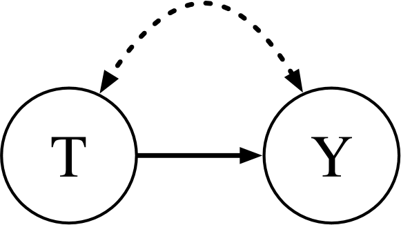
$$T_{i} =f_{T}(U_{i},\epsilon_{T_{i}};\theta)$$

$$Y_{i} =f_{Y}(T_{i},U_{i},\epsilon_{Y_{i}};\theta)$$

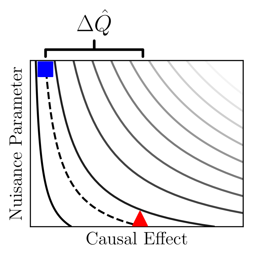
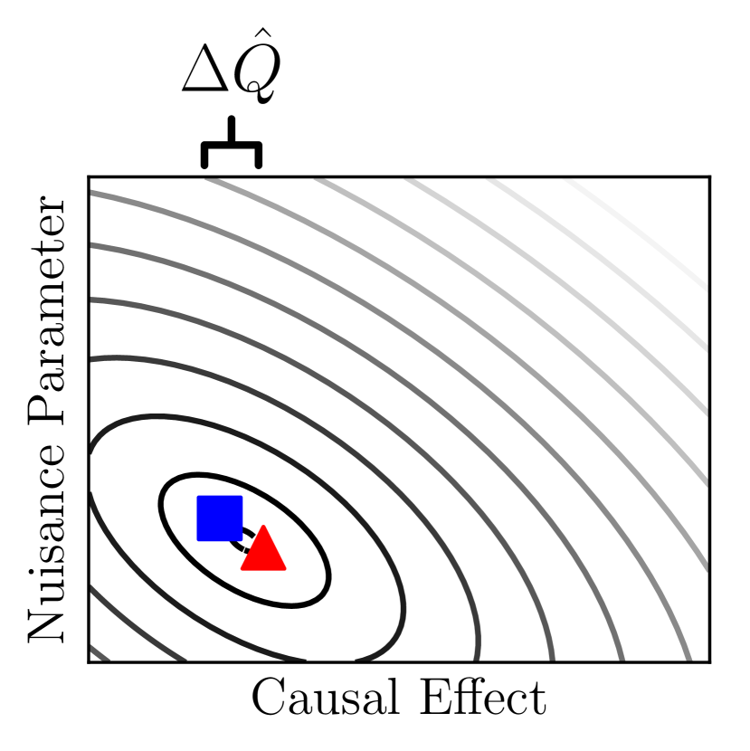
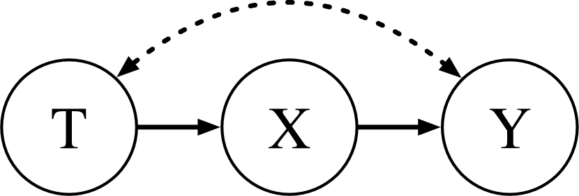
$$T_{i} =f_{T}(U_{i},\epsilon_{T_{i}};\theta)$$

$$X_{i} =f_{X}(T_{i},\epsilon_{X_{i}};\theta)$$

$$Y_{i} =f_{Y}(X_{i},U_{i},\epsilon_{Y_{i}};\theta)$$

(a)

(b)

Figure 1: Overview of simulation-based identiability. Simulation-based identifiability (SBI) recasts causal identifiability as an optimization problem that seeks to maximize the data likelihood and the distance, $\Delta\hat{Q}$, between the effect estimates induced by two sets of parameters, $\theta^{(1)}$ and $\theta^{(2)}$. When causal effects are not identifiable (a) SBI discovers maximum likelihood parameters (blue and red) that estimate different causal effects. When causal effects are identifiable (b) the two models converge to the same effect estimates.

1 Introduction

Drawing causal conclusions from data requires assumptions about underlying causal mechanisms (Pearl, 2009). Consequently, it is important to determine when these assumptions are sufficient to answer a causal query, i.e. whether the query is identifiable. Existing computational methods, such as the do-calculus, can rigorously determine identifiability from graph structure alone (Huang & Valtorta, 2006; Pearl, 1995), however, graph structure alone can be incomplete in some cases. For example, instrumental variable designs require an assumption of monotonicity or linearity (Cragg & Donald, 1993), within-subjects designs require an assumption that latent confounders are shared across units (Gelman, 2006; Loftus & Masson, 1994), and regression discontinuity designs violate positivity, an assumption required by the do-calculus (Lee & Lemieux, 2010).

A growing body of causal inference research employs assumptions that go beyond graph structure. For example, researchers in causal machine learning (Athey & Imbens, 2006; Hartford et al., 2017), and in hierarchical probabilistic modeling approaches to causal inference (Branson et al., 2019; Louizos et al., 2017; Tran & Blei, 2018; Witty et al., 2020b), have achieved promising results. Some of these techniques can be expressed as priors over structural causal models, and implemented as probabilistic programs.

Unfortunately, it is difficult to apply either analytical or graphical techniques to determine the identifiability of complex Bayesian approaches to causal inference. As a result, these approaches can produce inaccurate effect estimates even with infinite data (D’Amour, 2019; Rissanen & Marttinen, 2021). This paper introduces new automated techniques that can improve the rigor of causal inferences by providing simulation-based tests of identifiability (SBI).

SBI is compatible with any prior over structural causal models that: (i) can be used to sample data; and (ii) induces a differentiable likelihood function. The key innovation is to reduce causal identification to an optimization procedure that maximizes the likelihood of two sets of parameters while also maximizing the distance between their causal effect estimates. If the optimal solution is two sets of parameters that agree on effect estimates, then the effect is identifiable. See Figure 1 for intuition.

In Section 4, we prove that SBI is asymptotically sound and complete, assuming certain (strong) regularity conditions. In Section 5, we show that SBI is broadly applicable by presenting a suite of compatible benchmarks reflecting common graph-based and quasi-experimental designs. We show empirically that SBI correctly determines whether average treatment effects are identifiabile for all fourteen benchmarks. Finally, we use SBI to extract quantitive insight about Gaussian process regression discontinuity designs.

1.1 Related Work

Our work is not the first to automate identification for causal inference. Symbolic methods for observational (Huang & Valtorta, 2006; Pearl, 1995) and experimental (Lee et al., 2020) data determine whether queries are nonparametrically identifiable using graph structure alone. Similar methods have been developed for linear models (Bollen, 2005; Kumor et al., 2019). When applicable, symbolic methods like the do-calculus should be the de-facto choice, as they have strong theoretical gaurantees, are computationally efficient, and require minimal ancillary assumptions. However, these approaches are inconclusive for more flexible parameterizations, such as those using Gaussian processes, or models employing non-graphical assumptions, such as within-subjects designs. These methods (and SBI) do not attempt to test whether a set of assumptions are satisfied given a particular dataset. Instead, they test whether assumptions are sufficient to uniquely determine a causal effect from (yet unseen) data.

Similar approaches for determining identifiability have been developed in other fields, such as neuroscience (Valdes-Sosa et al., 2011) and dynamical systems (Raue et al., 2009), by searching for likelihood equivalent parameters using gradient-based search. SBI differs from these approaches in two important ways. First, SBI uses a particle-based objective function to search for likelihood equivalent models globally, rather than locally near a single maximum likelihood solution. Second, SBI’s objective function searches for models that estimate different causal effects, not only different parameters. This distinction means that SBI can correctly determine identifiability even when effects are composed of many parameters (e.g. see Section 4.1). It is well known that queries can be identified even in settings where individual parameters cannot (Pearl, 2009). Optimization techniques have been used to bound counterfactual queries (Balke & Pearl, 1994; Tian & Pearl, 2000; Zhang et al., 2021) or for neural-causal models (Xia et al., 2021), but do not support user-specified parametric assumptions.

Bayesian priors over parametric structural causal models can be implemented in probabilistic programming languages (Goodman et al., 2008; Mansinghka et al., 2014), which provide a syntax for expressing probabilistic models as code. Many of these languages support automatic differentiation and gradient-based optimization (Bingham et al., 2018; Carpenter et al., 2017; Cusumano-Towner et al., 2019; Dillon et al., 2017), providing the necessary utilities for our optimization-based approach. While some languages contain an explicit representation of interventions (Bingham et al., 2018; Perov et al., 2020; Tavares et al., 2019; Witty et al., 2020a), none currently address causal identifiabilty.

Design	Description	Source
Unconfounded	No latent variables influence both treatment, $T$, and outcome, $Y$.	(Pearl, 1995)
Confounded	A latent confounder, $U$, influences both $T$ and $Y$.	(Pearl, 1995)
Backdoor	An observed confounder, $X$, influences $T$ and $Y$.	(Pearl, 1995)
Frontdoor	$U$ influences $T$ and $Y$, but does not influence a mediator, $X$.	(Pearl, 1995)
Instrumental     variable	$U$ influences $T$ and $Y$. An observed instrument, $I$, influences $T$, does not influence $Y$ except through $T$, and is not influenced by $U$.	(Angrist et al., 1996)
Within subjects	Each instance of $U$ influences multiple instances of $T$ and $Y$.	(Draper, 1995)
Regression discontinuity	An observed confounder, $X$, influences $T$ and $Y$. $T$ is fully determined by $X$ being above or below a known threshold.	(Rubin, 1977)

Table 1: Description of quasi-experimental designs benchmarks. Of these seven standard causal designs, intrumental variable, within subjects, and regression discontinuity designs require assumptions that go beyond graph-structure. Parameterized versions of all seven designs can be represented as probabilistic programs, and can thus be tested using simulation-based identifiability.

2 Preliminaries

In this section we describe the necessary background on causal inference, and the Bayesian approach that SBI supports. Throughout this paper we use lowercase bold letters to denote arrays of random variables and uppercase letters with subscripts to denote their elements, e.g. $\textbf{u}_{1}=[U_{1,1},..,U_{1,n}]$. We use $Q$ interchangeably depending on context to denote either a causal query, e.g. sample average treatment effect, or the random variable induced by applying $Q$ to its random inputs.

Definition 2.1.

Structural Causal Models. A structural causal model (SCM) is a four-tuple $\textbf{M}=\langle\textbf{V},\textbf{E},\textbf{U},\textbf{F}\rangle$, where: $\textbf{V}=\{\textbf{t},\textbf{y},\textbf{x}_{1},...,\textbf{x}_{d}\}$ is a set of observed random variables, $\textbf{E}=\{\boldsymbol{\epsilon}_{\textbf{t}},\boldsymbol{\epsilon}_{\textbf{y}},\boldsymbol{\epsilon}_{\textbf{x}_{1}},...,\boldsymbol{\epsilon}_{\textbf{x}_{d}}\}$ is a set of independent exogenous latent variables, $\textbf{U}=\{\textbf{u}_{1},...,\textbf{u}_{d^{\prime}}\}$, is a set of latent confounders, and $\textbf{F}=\{f_{T},f_{Y},f_{X_{1}},...,f_{X_{d}}\}$ is a set of deterministic functions. Each observed variable is assigned according to its corresponding structural function, e.g. $Y_{i}=f_{Y}(T_{i},U_{1,i},\boldsymbol{\epsilon}_{Y_{i}})$. We use $Pa(\cdot)$ as shorthand for structural function arguments, e.g. $Pa(Y_{i})=\{T_{i},U_{1,i},\boldsymbol{\epsilon}_{Y_{i}}\}$. By construction, each $\boldsymbol{\epsilon}\in\textbf{E}$ is an argument of exactly one structural function, and each $\textbf{u}\in\textbf{U}$ is an argument of at least two structural functions. To represent an intervention, $do(T_{i}=t^{\prime})$, we replace the expression $T_{i}=f_{T}(Pa(T_{i}))$ with the expression $T_{i}=t^{\prime}$ and leave all other structural functions unchanged. We use $\textbf{V}^{\prime}$ to denote the set of counterfactual random variables $\{\textbf{y}^{\prime},\textbf{x}^{\prime}_{1},...,\textbf{x}^{\prime}_{d}\}$ induced by an intervention $do(T_{i}=t^{\prime})$ for all $i$ in $1,...,n$.

A growing body of literature (Louizos et al., 2017; Perov et al., 2020; Tavares et al., 2019; Tran & Blei, 2018; Witty et al., 2020a, b) has represented causal assumptions as a prior distribution over parametric SCMs, $p(\textbf{E},\textbf{F},\textbf{U})$. Here, practitioners do not claim that probability subsumes causal inference (Pearl, 2001), but instead that it represents uncertain belief over a class of (still causal) SCMs. This prior serves a conceptually similar role to a causal graph, restricting the space of SCMs a-priori (Bareinboim et al., 2020).

It is often convenient to reason about such priors in terms of observed endogenous variables, $p(\textbf{V},\textbf{F},\textbf{U})=p(\textbf{V}|\textbf{F},\textbf{U})p(\textbf{F},\textbf{U})$, marginalizing out exogenous noise. In this paper we assume that this pushforward, or change of variables, is tractable. For example, for the linear parameterization $Y_{i}=\beta T_{i}+\alpha U_{i}+\gamma\epsilon_{Y_{i}}$, $\epsilon_{Y_{i}}\sim\mathcal{N}(0,1)$, the conditional density $p(Y_{i}|f_{Y},U_{i})$ is given by $\mathcal{N}(Y_{i};\beta T_{i}+\alpha U_{i},\gamma)$.

Practitioners are rarely interested in counterfactual outcomes directly, and instead are interested in some causal query, $Q(\textbf{y},\textbf{y}^{\prime})$, such as the sample average treatment effect, $Q=\sum_{i=1}^{n}(Y^{\prime}_{i}-Y_{i})/n$. As in our linear example, where $Q=\beta(t^{\prime}-\sum_{i=1}^{n}T_{i})$, we assume that $Q$ is always fully determined by (V, F, U). Given data, the prior $p(\textbf{V},\textbf{F},\textbf{U})$ and the causal query $Q$ induces a posterior density over causal effects, $p(Q|\textbf{V})$, as follows, where $\mathcal{A}$ is the set of all tuples $(\textbf{F},\textbf{U})$ that induce a causal effect $Q$:

$$p(Q|\textbf{V})=\dfrac{1}{p(\textbf{V})}\int_{(\textbf{F},\textbf{U})\in\mathcal{A}}p(\textbf{V}|\textbf{F},\textbf{U})\;dp(\textbf{F},\textbf{U})$$ (1)

Priors over Structural Functions.

As it is impossible to define a prior over all functions $f:\mathbb{R}\to\mathbb{R}$ (Aumann, 1961), we restrict our attention to structural functions that are fully specified by a finite collection of parameters, $\theta\in\mathbb{R}^{d}$, with a corresponding prior, $p(\theta)$. While this appears to be restrictive, this template covers a broad range of models, from linear models to Bayesian neural networks (Neal, 2012). As an example, in Section 4.1 we show how SBI can be used to reason about SCMs with Gaussian process priors (Rasmussen, 2003), i.e. distributions over deterministic functions, $Y_{i}=f(X_{i})=\phi(X_{i})^{t}\textbf{w}$, $\textbf{w}\sim\mathcal{N}(\mu,\Sigma)$, where $\phi$ is some basis function.

3 Identifiability in Bayesian Causal Inference

In this work we are interested in understanding the key asymptotic properties of $p(Q|\textbf{V})$, namely whether posterior mass concentrates around the true causal effect assymptotically. In other words, can the causal effect be identified from data? We define $\eta$-identifiability in this setting as follows:

Definition 3.1.

$\mathbf{\eta}$-identifiability. Let $(\tilde{\textbf{F}},\tilde{\textbf{U}})$ be a set of structural functions and latent confounders in the support of the prior, $p(\textbf{F},\textbf{U})$. Then, a causal query, $Q$, is $\eta$-identifiable given $(\tilde{\textbf{F}},\tilde{\textbf{U}})$ if for a dataset of $n$ instances, $\tilde{\textbf{V}}\sim p(\textbf{V}|\tilde{\textbf{F}},\tilde{\textbf{U}})$, $\mathbb{P}(|\tilde{Q}-Q|\leq\eta|\tilde{\textbf{V}})\to 1$ for some $\eta\in\mathcal{R^{+}}$ almost surely as $n\to\infty$, where $\tilde{Q}$ is the causal effect induced by $(\tilde{\textbf{F}},\tilde{\textbf{U}},\tilde{\textbf{V}})$.

Even though Definition 3.1 is given in terms of an intractable posterior distribution, determining whether a causal effect is $\eta$-identifiable does not require computation or approximation of the posterior directly. Instead, we show that a causal query is $\eta$-identifiable if and only if there do not exist a set of maximum likelihood structural functions and latent confounder in the support of the prior, $(\textbf{F}^{\prime},\textbf{U}^{\prime})$, that induce causal effects that differ from $(\tilde{\textbf{F}},\tilde{\textbf{U}})$ by more than $\eta$. Proofs of all theorems are provided in the supplementary materials.

Theorem 3.1.

$Q$ is $\eta$-identifiable given $(\tilde{\textbf{F}},\tilde{\textbf{U}})$ if and only if for a dataset of $n$ instances, $\tilde{\textbf{V}}\sim p(\textbf{V}|\tilde{\textbf{F}},\tilde{\textbf{U}})$, there does not exist an $(\textbf{F}^{\prime},\textbf{U}^{\prime})$ such that $p(\tilde{\textbf{V}}|\textbf{F}^{\prime},\textbf{U}^{\prime})=p(\tilde{\textbf{V}}|\tilde{\textbf{F}},\tilde{\textbf{U}})$, $|\tilde{Q}-Q^{\prime}|>\eta$, and $p(\textbf{F}^{\prime},\textbf{U}^{\prime})/p(\tilde{\textbf{F}},\tilde{\textbf{U}})>0$ almost surely as $n\to\infty$. Here, $\tilde{Q}$ and $Q^{\prime}$ are the causal effects induced by $(\tilde{\textbf{F}},\tilde{\textbf{U}},\tilde{\textbf{V}})$ and $(\textbf{F}^{\prime},\textbf{U}^{\prime},\tilde{\textbf{V}})$ respectively.

Definition 3.1 describes identifiability with respect to a single instantiation, $(\tilde{\textbf{F}},\tilde{\textbf{U}})$. Instead, we would like to make statements about whether causal effects can be uniquely identified with high probability across SCMs sampled from the prior. Let $\textrm{ID}(\tilde{\textbf{F}},\tilde{\textbf{U}},\eta)$ be a function that returns $1$ if $Q$ is $\eta$-identifiable given $(\tilde{\textbf{F}},\tilde{\textbf{U}})$ under Definition 3.1, and $0$ otherwise. Then, we define $(\zeta,\eta)$-identifiability as follows:

Definition 3.2.

$\mathbf{(\zeta,\eta)}$-identifiability. For some $0\leq\zeta\leq 1$, $\eta\in\mathbb{R}^{+}$, a causal query, $Q$, is $(\zeta,\eta)$-identifiable given a prior distribution $p(\textbf{F},\textbf{U})$ if the probability that $Q$ is $\eta$-identifiable given a $(\tilde{\textbf{F}},\tilde{\textbf{U}})\sim p(\textbf{F},\textbf{U})$ is greater than or equal to $\zeta$, i.e. $\zeta\leq\int\textrm{ID}(\tilde{\textbf{F}},\tilde{\textbf{U}},\eta)\;dp(\tilde{\textbf{F}},\tilde{\textbf{U}})$.

3.1 Example: Confounded Linear Model

Here, we illustrate the Bayesian approach with a linear parametric example over observed $\textbf{V}=\{\textbf{t},\textbf{y}\}$ and latent $\textbf{U}=\{\textbf{u}\}$ and $\textbf{E}=\{\boldsymbol{\epsilon}_{t},\boldsymbol{\epsilon}_{y}\}$, which is a simplified version of the example in Section 5 of (D’Amour, 2019). This example corresponds to the graphical structure shown in Figure LABEL:fig:not_id_contour. Here, the structural causal model is parameterized by $\theta=\{\gamma,\beta,\alpha,\sigma_{U}^{2},\sigma_{T}^{2},\sigma_{Y}^{2}\}$. Assume the following SCM:

$$U_{i} \sim\mathcal{N}(0,\sigma_{U}^{2}) T_{i} =\gamma U_{i}+\epsilon_{T_{i}} Y_{i} =\beta T_{i}+\alpha U_{i}+\epsilon_{Y_{i}}$$

$$\epsilon_{T_{i}} \sim\mathcal{N}(0,\sigma_{T}^{2}) \epsilon_{Y_{i}} \sim\mathcal{N}(0,\sigma_{Y}^{2})$$

Let our causal query again be the sample average treatment effect (SATE), i.e. $Q(\textbf{y},\textbf{y}^{\prime})=\beta(t^{\prime}-\sum_{i=1}^{n}T_{i})$. In this setting, estimating the causal effect reduces to estimating $\beta$. As shown in (D’Amour, 2019), for all $\tilde{\textbf{V}}$ in the support of $p(\textbf{V})$ there exists a set of parameters $\Theta$ such that for all $\theta^{(1)},\theta^{(2)}\in\Theta$, $\beta^{(1)}\neq\beta^{(2)}$ and $p(\tilde{\textbf{V}}|\theta^{(1)})=p(\tilde{\textbf{V}}|\theta^{(2)})$. In summary, the induced linear system of equations relating parameters to the observable covariance between t and y is rank deficient, leading to non-uniqueness of the maximum likelihood solution. This implies that the posterior odds ratio, $p(\beta^{(1)}|\tilde{\textbf{V}})/p(\beta^{(2)}|\tilde{\textbf{V}})$, reduces to the prior odds ratio, $p(\beta^{(1)})/p(\beta^{(2)})$, regardless of $n$ (Witty et al., 2020b). It follows straightforwardly that given any nondegenerate prior, $p(\theta)$, $Q$ is therefore not $(\zeta,\eta)$-identifiable for any $0\leq\zeta\leq 1$, $\eta\in\mathbb{R}^{+}$. This conclusion agrees with known parametric identification results (Pearl, 2009).

Algorithm 1 Simulation-Based Identifiability (SBI)

1:  procedure $\textrm{SBI}(p(\textbf{F},\textbf{U},\textbf{V}),Q,\eta,\zeta)$

2:     parameters: $m$, SCM samples; $n$; dataset size; $k$, data samples; $\lambda$, repulsion strength, $\alpha$, significance level

3:     for $i=1$ to $m$ do

4:        $\tilde{\textbf{F}}_{i},\tilde{\textbf{U}}_{i}\sim p(\textbf{F},\textbf{U})$                                    $\triangleright$ Sample structural functions and $n$ confounder instances from the prior

5:        for $j=1$ to $k$ do

6:           $\tilde{\textbf{V}}_{i,j}\sim p(\textbf{V}|\tilde{\textbf{F}}_{i},\tilde{\textbf{U}}_{i})$                                                                      $\triangleright$ Sample $n$ observations from the $i$’th SCM

7:           $\Delta\hat{Q}_{i,j}\leftarrow\textrm{Optimize }\mathcal{L}(\cdot,\tilde{\textbf{V}}_{i,j};\lambda)$                                      $\triangleright$ Using stochastic gradient descent. See Equation 2

8:        end for

9:        $\hat{\mu}_{i}\leftarrow\sum_{j=1}^{k}\Delta\hat{Q}_{i,j}/k$                                                                             $\triangleright$ Compute sample mean for $i$’th SCM

10:        $\hat{S}_{i}\leftarrow\sum_{i=1}^{k}(\hat{\mu}_{i}-\Delta\hat{Q}_{i,j})^{2}/(k-1)$                                                    $\triangleright$ Compute sample variance for $i$’th SCM

11:     end for

12:     $l_{0}\leftarrow\max_{\zeta^{\prime}\in[0,\zeta]}\sum_{i=1}^{m}\log(\mathcal{N}(\hat{\mu}_{i};\min(\hat{\mu}_{i},\eta),\hat{S}_{i}/k)\zeta^{\prime}+\mathcal{N}(\hat{\mu}_{i};\max(\hat{\mu}_{i},\eta),\hat{S}_{i}/k)(1-\zeta^{\prime}))$   $\triangleright$ Null log likelihood

13:     $l_{a}\leftarrow\max_{\zeta^{\prime}\in[0,1]}\sum_{i=1}^{m}\log(\mathcal{N}(\hat{\mu}_{i};\min(\hat{\mu}_{i},\eta),\hat{S}_{i}/k)\zeta^{\prime}+\mathcal{N}(\hat{\mu}_{i};\max(\hat{\mu}_{i},\eta),\hat{S}_{i}/k)(1-\zeta^{\prime}))$   $\triangleright$ Alt. log likelihood

14:     return TRUE if $\chi^{2}(2(l_{a}-l_{0});1)<\alpha$ else return FALSE                   $\triangleright$ Chi-squared test of statistical significance

4 Simulation-Based Identifiability

For the linear example in Section 3.1, we were able to relate the observable covariance between t and y to the latent parameters $\theta$ algebraically. However, it is not clear how we might derive similar results for nonlinear structural functions in general. Instead, we propose an approach for determining causal identifiability using a particle-based optimization scheme which we call simulation-based identifiability (SBI). In summary, SBI uses gradient-based search to find two sets of maximum likelihood structural functions and latent confounders in the support of $p(\textbf{F},\textbf{U})$, $(\textbf{F}^{(1)},\textbf{U}^{(1)})$ and $(\textbf{F}^{(2)},\textbf{U}^{(2)})$, that induce different causal effects, $Q^{(1)}$ and $Q^{(2)}$, respectively. Let $\lambda\in\mathcal{R^{+}}$ be a hyperparameter and $\Delta Q\coloneqq|Q^{(1)}-Q^{(2)}|$. Then, consider the following objective function:

$$\mathcal{L} (\underbrace{\textbf{F}^{(1)},\textbf{U}^{(1)}}_{\textrm{SCM 1}},\underbrace{\textbf{F}^{(2)},\textbf{U}^{(2)}}_{\textrm{SCM 2}},\underbrace{\tilde{\textbf{V}}\vphantom{g}}_{\textrm{Data}};\lambda)$$ (2)

$$=\underbrace{\log p(\tilde{\textbf{V}}|\textbf{F}^{(1)},\textbf{U}^{(1)})}_{\textrm{SCM 1 log likelihood}}+\underbrace{\log p(\tilde{\textbf{V}}|\textbf{F}^{(2)},\textbf{U}^{(2)})}_{\textrm{SCM 2 log likelihood}}+\underbrace{\lambda\Delta Q}_{\textrm{Repulsion}}$$

Let $\hat{\textbf{F}}^{(1)},\hat{\textbf{U}}^{(1)},\hat{\textbf{F}}^{(2)},\hat{\textbf{U}}^{(2)}$ denote a solution that maximizes $\mathcal{L}$, and let $\Delta\hat{Q}$ be the corresponding optimal $\Delta Q$. The following asymptotic theorems hold for any $\lambda\in\mathbb{R}^{+}$ and bounded $Q$:

Theorem 4.1.

A causal query $Q$ is $\eta$-identifiable given $(\tilde{\textbf{F}},\tilde{\textbf{U}})$ for a dataset of $n$ instances, $\tilde{\textbf{V}}\sim p(\textbf{V}|\tilde{\textbf{F}},\tilde{\textbf{U}})$, if $\Delta\hat{Q}\leq 2\eta$ and only if $\Delta\hat{Q}\leq\eta$ almost surely as $n\to\infty$.

Theorem 4.2.

A causal query $Q$ is $(\zeta,\eta)$-identifiable given a prior $p(\textbf{F},\textbf{U})$ for $m$ samples of functions and confounders, $\tilde{\textbf{F}}_{i},\tilde{\textbf{U}}_{i}\sim p(\textbf{F},\textbf{U})$, and $m$ datasets of $n$ instances, $\tilde{\textbf{V}}_{i}\sim p(\textbf{V}|\tilde{\textbf{F}}_{i},\tilde{\textbf{U}}_{i})$, if $\zeta<\sum_{i=1}^{m}\mathbbm{1}_{\Delta\hat{Q}_{i}>2\eta}$ and only if $\zeta<\sum_{i=1}^{m}\mathbbm{1}_{\Delta\hat{Q}_{i}>\eta}$ almost surely as $n,m\to\infty$.

Theorems 4.1 and 4.2 provide necessary and sufficient conditions for determining identifiability in the limit of infinite simulations given exact solutions to $\mathcal{L}$. However, given finite $n$ and $m$ and approximate solutions to $\mathcal{L}$, $\Delta\hat{Q}$ may be large even if the query is identifiable. To address the problem of finite $n$ and $m$ we propose a likelihood ratio hypothesis test using gradient-based approximate solutions to $\mathcal{L}$. The details of this procedure are shown in Algorithm 1, which works as follows. Repeatedly sample a set of functions and latent confounders, $(\tilde{\textbf{F}},\tilde{\textbf{U}})$, from the prior. For each, repeatedly sample a set of observations, $\tilde{\textbf{V}}$, and optimize $\mathcal{L}$ jointly for two SCMs, resulting in an approximately optimal $\Delta\hat{Q}$ for the simulated data. Then, apply a likelihood ratio test to determine if the distance between particles is statistically significantly greater than $\eta$ with probability $\zeta$.

Theorem 4.3.

For convex $\mathcal{L}$, Algorithm 1 approaches the most powerful exact test with significance $\alpha$ as $n,k\to\infty$.

For finite $k$, where the central limit theorem does not provide an exact description of the distribution of the sample mean $\hat{\mu}_{i}$, this procedure is best described as an approximate test. See the supplementary materials for additional details about the likelihood ratio test. While gradient-based optimization is not gauranteed to escape local optima, our many experiments in Section 5 suggest that SBI is robust even when $\mathcal{L}$ is non-convex and for finite $n$, $m$, and $k$. SBI correctly determines identifiability for all six of our latent variable model benchmarks, which we strongly suspect all have non-convex likelihoods. We believe that approximate solutions to $\mathcal{L}$ are reliable in practice for two reasons. First, SBI aggregates $m\cdot k$ independent runs of gradient-based optimization on simulated data in its statistical test. For example, even though 14 of the 5000 trajectories had $\Delta\hat{Q}>\eta$, SBI concluded that SATE for the linear IV benchmark is identifiable. Second, SBI uses stochastic gradients and modern optimizers (e.g., Adam) that are known to escape local optima in non-convex high-dimensional settings.

Selecting the repulsion strength, $\lambda$.

While the choice of repulsion strength, $\lambda$, does not influence our asymptotic results, this is not generally the case for any finite $n$. In our experiments in Section 5, we find that even small values of $\lambda$ produce large $\Delta\hat{Q}$ for non-identifiable models.

4.1 Example: Confounded Gaussian Process

Let us again consider the confounded model in Section 3.1, instead assuming that the function $Y_{i}=f(T_{i},U_{i},\epsilon_{Y_{i}})$ is drawn from the following Gaussian process prior over $Y_{i}=\mu_{Y}(T_{i},U_{i})+\sigma^{2}_{Y}\epsilon_{Y_{i}}$, where $D\in\mathbb{N}$, $\boldsymbol{\mu}_{Y}=[\mu_{Y}(T_{1},U_{1}),...,\mu_{Y}(T_{n},U_{n})]$, and $\textbf{w}=\{\sigma^{2}_{Y},w_{0},w_{1,1},...,w_{4,1},...,w_{1,D},...,w_{4,D}\}$:

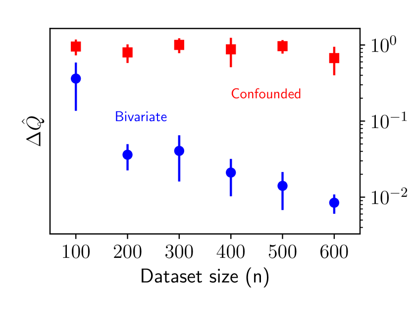
(a) Gaussian Process

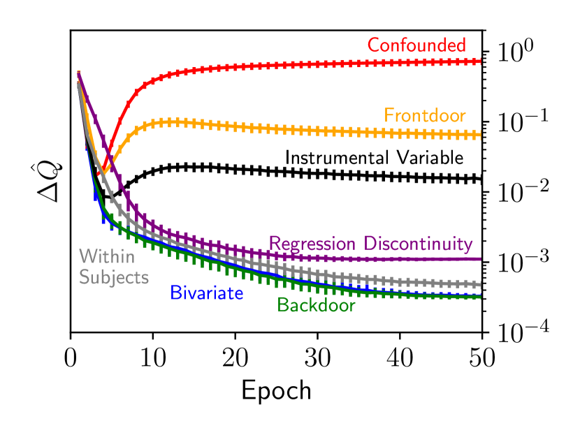
(b) Linear Training Curves

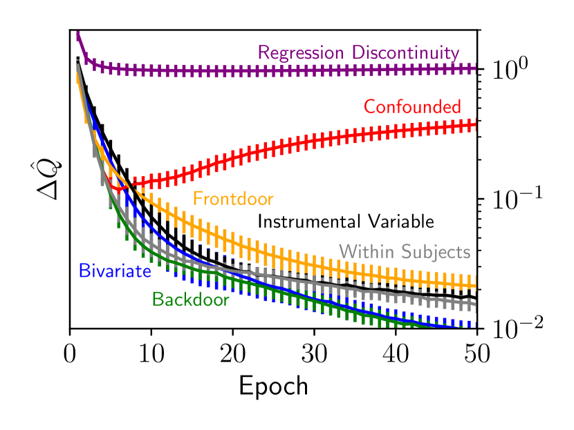
(c) Gaussian Process Training Curves

Figure 2: Summaries of particle-based optimization. As the simulated dataset size increases the difference between effect estimates of the two particles ($\Delta\hat{Q}$) remains large for the confounded Gaussian process model (a), indicating that the model is not identifiable. Without confounding however, the optimized particles converge to the same causal effect. Using gradient-based optimization, SBI is able to discover likelihood equivalent causal models when they exist that induce different effects for linear (b) and Gaussian process (c) models.

$$\mu_{Y}(T_{i},U_{i})=w_{0}+\sum_{d=1}^{D} w_{1,d}\sin(dT_{i})+w_{2,d}\cos(dT_{i})$$

$$+w_{3,d}\sin(dU_{i})+w_{4,d}\cos(dU_{i})$$

This Gaussian process model is known as the Fourier model, where the choice of $D$ and the prior $p(\textbf{w})$ dictate the characteristics of the sampled functions (Rasmussen & Ghahramani, 2001). In this and all subsequent experiments we set $D=10$, $w_{0}\sim\mathcal{N}(0,1)$, and $w_{1,d},w_{2,d},w_{3,d},w_{4,d}\overset{iid}{\sim}\mathcal{N}(0,1/d^{2})$. This choice of prior results in relatively smooth functions, as the weights on higher-order terms are typically close to 0. Again, let the causal query, $Q$, be the sample average treatment effect with the intervention $do(T_{i}=t^{\prime})$. Then the log likelihood and the difference between causal effects are given by the following:

$$\begin{gathered}\begin{aligned} \log{p(\textbf{V}|\textbf{F},\textbf{U})}&=\log{\mathcal{N}(\textbf{t};\gamma\textbf{u},\sigma^{2}_{T}\textbf{I})}+\log{\mathcal{N}(\textbf{y};\boldsymbol{\mu}_{Y},\sigma^{2}_{Y}\textbf{I})}\end{aligned}\\ \begin{aligned} \Delta Q&=\sum_{d=1}^{D}|w_{1,d}^{(1)}-w_{1,d}^{(2)}|\sin(dt^{\prime})+|w_{2,d}^{(1)}-w_{2,d}^{(2)}|\cos(dt^{\prime})\end{aligned}\end{gathered}$$

Given this expressions for the log likelihood and the causal query in terms of parameters, $\theta$, and latent confounders, U, we can now compute the partial derivative of the particle-based objective function, $\frac{\partial}{\partial s}\mathcal{L}=\frac{\partial}{\partial s}\log{p(\tilde{\textbf{V}}|\textbf{F}^{(1)},\textbf{U}^{(1)})}+\frac{\partial}{\partial s}\log{p(\tilde{\textbf{V}}|\textbf{F}^{(2)},\textbf{U}^{(2)})}+\lambda\frac{\partial}{\partial s}\Delta Q$ with respect to all $s\in\theta\cup\textbf{U}$. Given an expression for each partial derivative, we can then apply standard gradient-descent algorithms to determine identifiability using SBI. Without loss of generality, the derivative of the repulsion term with respect to $s$ for $\textbf{F}^{(1)}$, $\textbf{U}^{(1)}$ is given by the following:

$$\frac{\partial}{\partial s}\Delta Q=\begin{cases}\dfrac{w_{1,d}^{(1)}-w_{1,d}^{(2)}}{|w_{1,d}^{(1)}-w_{1,d}^{(2)}|}\sin(dt^{\prime})&s=w_{1,d}^{(1)}\\ \dfrac{w_{2,d}^{(1)}-w_{2,d}^{(2)}}{|w_{1,d}^{(1)}-w_{2,d}^{(2)}|}\cos(dt^{\prime})&s=w_{2,d}^{(1)}\\ 0&\textrm{otherwise}\end{cases}$$

For the derivative of the log density we expand on standard identities of Gaussians, where $L_{\textbf{V}}$, $L_{\textbf{t}}$, and $L_{\textbf{y}}$ are shorthand for $\log{p(\textbf{V}|\textbf{F}^{(1)},\textbf{U}^{(1)})}$, $\log{p(\textbf{t}|\gamma\textbf{U},\sigma_{T}^{2}\textbf{I})}$, and $\log{\mathcal{N}(\textbf{y};\boldsymbol{\mu}_{Y},\sigma^{2}_{Y}\textbf{I})}$ respectively:

$$\frac{\partial L_{\textbf{V}}}{\partial s} =\frac{\partial L_{\textbf{t}}}{\partial s}+\frac{\partial L_{\textbf{y}}}{\partial s}$$

See the supplementary materials for additional details on the remaining partial derivatives. Note that although deriving these gradients is cumbersome and error-prone in general, it can be easily automated using standard automatic differentiation procedures.

Design	Prior	$\Delta\hat{Q}_{\textrm{SBI}}$	$\Delta\hat{Q}_{\textrm{PL}}$	$\Delta\hat{Q}_{\textrm{MH}}$	$\textrm{ID}_{\textrm{Truth}}$	$\textrm{ID}_{\textrm{SBI}}$	$\textrm{ID}_{\textrm{PL}}$	$\textrm{ID}_{\textrm{MH}}$	$\textrm{ID}_{\textrm{DAG}}$
Unconfounded	Linear	.00 $\pm$ .00	.11 $\pm$ .01	.12 $\pm$ .03	green✓	green✓	red✗	red✗	green✓
	GP	.01 $\pm$ .00	.34 $\pm$ .02	.26 $\pm$ .06	green✓	green✓	red✗	red✗	green✓
Confounded	Linear	.83 $\pm$ .15	1.8 $\pm$ .34	.14 $\pm$ .03	red✗	red✗	red✗	red✗	red✗
	GP	.50 $\pm$ .28	.73 $\pm$ .14	.38 $\pm$ .08	red✗	red✗	red✗	red✗	red✗
Backdoor	Linear	.00 $\pm$ .00	.10 $\pm$ .01	.11 $\pm$ .02	green✓	green✓	red✗	red✗	green✓
	GP	.01 $\pm$ .00	.28 $\pm$ .02	.26 $\pm$ .05	green✓	green✓	red✗	red✗	green✓
Frontdoor	Linear	.06 $\pm$ .04	.17 $\pm$ .05	.37 $\pm$ .13	green✓	green✓	red✗	red✗	green✓
	GP	.02 $\pm$ .01	.20 $\pm$ .09	.34 $\pm$ .17	green✓	green✓	red✗	red✗	green✓
Instrumental variable	Linear	.01 $\pm$ .01	.05 $\pm$ .01	.13 $\pm$ .06	green✓	green✓	green✓	red✗	green✓
	GP	.01 $\pm$ .00	.37 $\pm$ .03	.40 $\pm$ .08	green✓	green✓	red✗	red✗	red✗
Within subjects	Linear	.00 $\pm$ .00	.10 $\pm$ .01	.14 $\pm$ .03	green✓	green✓	red✗	red✗	red✗
	GP	.01 $\pm$ .01	.39 $\pm$ .04	.26 $\pm$ .06	green✓	green✓	red✗	red✗	red✗
Regression discontinuity	Linear	.00 $\pm$ .00	.16 $\pm$ .01	.21 $\pm$ .03	green✓	green✓	red✗	red✗	green✓
	GP	1.1 $\pm$ .12	1.1 $\pm$ .09	.82 $\pm$ .1	red✗	red✗	red✗	red✗	green✓

Table 2: Empirical results on quasi-experimental design benchmarks. Simulation-based identifiability (this paper) correctly determines the identifiability of sample average treatment effects for all fourteen of the benchmark linear and Gaussian process (GP) quasi-experimental designs. Lower $\Delta\hat{Q}$ implies identifiability. The columns labeled ID show whether SBI and the baselines determine the design to be statistically significantly identifiable. Neither of the profile likelihood (PL) or the Metropolis Hastings (MH) baselines consistently determine identifiability. The column labeled $\textrm{ID}_{\textrm{DAG}}$ presents the results of the do-calculus (Pearl, 1995) for GP benchmarks, and IC (Kumor et al., 2019) for linear benchmarks applied (incorrectly) to the underlying causal graphs, despite the fact that they do not account for all of the parametric restrictions. This comparison is only to illustrate the effect of parametric restrictions on identifiability.

Figure 2(a) shows the results of Algorithm 1 with this prior over structural causal models using the Adam gradient descent algorithm (Kingma & Ba, 2015) to optimize $\mathcal{L}$. Unlike the unconfounded model, which is identical except that U has been omitted, we conclude that the confounded model is not identifiable. We expand on these examples in Section 5.

5 Experiments

We evaluated SBI on a benchmark suite of priors reflecting seven standard causal designs which are summarized in Table 1; unconfounded regression, confounded regression, backdoor adjusted, frontdoor adjusted, instrumental variable, within-subjects, and regression discontinuity designs. For each of these seven benchmarks we tested SBI using a linear parameterization (e.g. Section 3.1) as well as a parameterization where the outcome function is replaced with a Gaussian process (e.g. Section 4.1). Additional experimental details and descriptions of each prior are provided in the supplementary materials.

We compared SBI against two baselines, one which seeks to approximate the full posterior directly using a Metropolis-Hastings based inference procedure (MH), and one which uses a variation of profile likelihood (PL) identification (Raue et al., 2009), which alternates between parameter perturbations and maximum-likelihood optimization. We implemented Algorithm 1, all designs, and the baselines using the Gen probabilistic programming language (Cusumano-Towner et al., 2019), which provides the necessary support for sampling and automatic differentiation. Using $m=100$, $n=1000$, $k=50$, $\lambda=1$, $\eta=0.1$, $\zeta=0.8$, and $\alpha=0.05$, SBI correctly determines the identifiability of all designs, performing significantly better than the two baselines. As we formalized in Section 4, if $\Delta\hat{Q}$ is close to $0$ then the causal query is identifiable.

Our experiments demonstrate that SBI agrees with the do-calculus in settings where graph structure alone is sufficient, and produces correct identification results for designs that previously required custom identification proofs. Finally, we present the first known identification results for Gaussian process quasi-experimental designs, demonstrating agreement with widely held intuition. See Table 2 for a summary of SATE identification results.

Causal graphical models.

In addition to the unconfounded and confounded regression designs presented in Section 4.1, we evaluated SBI on two models that are covered by the do-calculus, backdoor-adjusted and frontdoor-adjusted designs. Backdoor-adjusted designs represent settings where all of the random variables that confound the relationship between treatment and outcome are observed, blocking all backdoor paths. Unlike backdoor-adjusted designs, frontdoor-adjusted designs can include latent confounding between treatment and outcome, as long as there exists an observed mediator that is not confounded, as in Figure LABEL:fig:id_contour. Despite this latent confounding, average treatment effects are nonparametrically identifiable (Pearl, 2009).

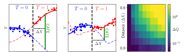
(a)

(b)

(c)

Figure 3: Quantitative insight for conditional average treatment effects. SBI provides novel and intuitive identification results for the Gaussian process regression discontinuity design benchmark. These results (c) show that conditional average treatment effects (CATE) becomes less identifiable as we condition on covariates further from the discontinuity $(\Delta X>0)$ and for less smooth outcome functions, i.e. increasing the number of basis functions (a, b).

Linear Quasi-Experimental Designs.

Instrumental variable designs differ from the confounded design in that an observed variable, known as the instrument, influences the treatment. Two conditions must be satisfied to enable identification: (i) the instrument and the treatment must not be confounded; and (ii) all influence from the instrument to the outcome is mediated through the treatment. While these assumptions can be expressed graphically, additional parametric assumptions are needed for effects to be identifiable (Pearl, 2009). For example, if exogenous noise is additive, then the average treatment effect is identifiable (Hartford et al., 2017).

Within-subjects designs involve hierarchically structured data in which individual instances (e.g., students) are affiliated with one of several objects (e.g., schools). Treatment effects for these kinds of settings can be identified even if treatment and outcome are confounded, as long as confounders are shared across all instances belonging to the same object (Witty et al., 2020b). These designs can be described as the family of structural causal models; $T_{i}=f_{T}(U_{o(i)},\epsilon_{T_{i}})$ $Y_{i}=f_{Y}(T_{i},U_{o(i)},\epsilon_{Y_{i}})$, where $U_{o(i)}$ refers to the shared value of the latent confounder corresponding to instance $i$. Hierarchically structured confounding is applicable to a wide variety of common causal designs (Jensen et al., 2020): including twin studies (Boomsma et al., 2002), difference-in-differences designs (Shadish et al., 2008), and multi-level-modeling (Gelman, 2006).

Regression discontinuity designs are quasi-experimental designs in which the treatment depends on a particular observed covariate being above or below a known threshold. We consider a sharp deterministic discontinuity, i.e. $T_{i}=1$ if $X_{i}>0$, and $T_{i}=0$ otherwise. These regression discontinuity designs correspond to the family of structural causal models $X_{i}=f_{X}(\epsilon_{X_{i}})$, $T_{i}=\mathbbm{1}_{X_{i}>0}$, and $Y_{i}=f_{Y}(T_{i},X_{i},\epsilon_{T_{i}})$. Even though all confounders are observed, the deterministic relationship between $X$ and $T$ violates the positivity assumption, which is a necessary assumption for the do-calculus to be sound (Pearl, 1995). Here, average treatment effects are identifiable for linear models, but not nonparametrically.

Gaussian Process Quasi-Experimental Designs.

We used SBI to determine the previously unknown identifiability of Gaussian process versions of quasi-experimental designs. By assuming a particular kernel we place an inductive bias on the class of structural functions, which could in principle enable identification. SBI instead confirms that the identifibility of these Gaussian process models agrees with the literature on nonparameteric identification.

We also evaluated SBI on the conditional average treatment effect (CATE) for a Gaussian process version of the regression discontinuity design. For nonlinear outcome functions, such as our Gaussian process, observations in one region of $X$ provide only partial information about counterfactuals in another. For example, in Figure LABEL:fig:rdd_nonsmooth the outcome function for untreated individuals ($T=0$) to the right of the discontinuity (dashed blue curve) is only one of many that are compatible with observed data. Therefore, we should expect that CATE is more ambiguous further from the discontinuity and for less smooth functions. SBI’s results in Figure LABEL:fig:rdd_cate_results agree with this intuition, demonstrating that $\Delta Q$ increases as we condition on covariates further from the discontinuity and as we increase the number of basis functions.

6 Discussion

In this paper we demonstrated how SBI can be used to test the identifiability of Bayesian models for causal inference. While determining identifiability is particularly salient in these causal settings, it can also be valuable in non-causal settings as a part of a holistic modeling workflow (Gelman et al., 2020), supplementing other introspection tools such as simulation-based calbration (Talts et al., 2018).

In addition to determining identifiability, SBI can be used as a kind of sensitivity analysis (Franks et al., 2019; Kallus et al., 2019; Robins et al., 2000), bounding the range of causal effects that are likelihood equivalent. Our regression discontinuity design results shown in Figure LABEL:fig:rdd_cate_results emphasize this capability, showing that irreducible uncertainty in effect estimates increases with increasing distance from the discontinuity and with less smooth outcome functions.

Our benchmarks encode strong parametric assumptions about latent confounders and exogenous noise. If desired, users may represent broader uncertainty using hyperpriors. To demonstrate this, we ran a version of the confounded GP model with additional hyperpriors over the mean and variance of $U$. See the supplementary materials for details. As another example, one could relax additive noise assumptions using Bayesian versions of invertible neural networks (Dinh et al., 2016), which satisfy SBI’s requirements that the likelihood be differentiable and that counterfactual outcomes (and thus $Q$) are fully determined by $(\textbf{F},\textbf{U},\textbf{V})$.

SBI builds on a long history of optimization-focused machine learning research. Reducing identifiability to optimization in this way provides a path towards reasoning about Bayesian models for causal inference at previously unattainable scales. However, this reduction means that SBI’s conclusions are dictated by the performance of an approximate global optimization method. Formally quantifying the implications of this approximation error, and extending SBI to discrete combinatorial causal models (e.g. causal discovery) are important areas of future work.

Appendix A Structural Causal Models

Here, we present a mathematical description for the structural causal models underlying the unconfounded regression and the backdoor adjusted designs which is agnostic to any particular choice of functions, which we expand on for particular choices of functions in Section B of this supplementary materials. The remaining five designs in Table 1 are presented throughout the main body of the paper.

Unconfounded Regression.

The unconfounded regression design is identical to the confounded regression design, except that the latent confounded has been omitted. Specifically, we have that $T_{i}=f_{T}(\epsilon_{T_{i}})$ and $Y_{i}=f_{Y}(T_{i},\epsilon_{Y_{i}})$.

Backdoor Adjusted Design.

The backdoor adjusted design includes an observed confounder, $X$, that influence both treatment, $T$, and outcome $Y$, but no latent confounders. Specifically, we have that $X_{i}=f_{X}(\epsilon_{X_{i}})$, $T_{i}=f_{T}(X_{i},\epsilon_{T_{i}})$, and $Y_{i}=f_{Y}(T_{i},X_{i},\epsilon_{Y_{i}})$.

Appendix B Experiments

In this section we provide additional detail for the linear and Gaussian process experiments. For each of the seven designs we assume that treatment, $T$, outcome, $Y$, and where applicable covariates, $X$, and instruments, $I$, are observed. All other random variables are latent.

For all of the experiments we used the Adam (Kingma & Ba, 2015) algorithm to optimize $\mathcal{L}$. We ran Adam with $\alpha=0.01$, $\beta_{1}=0.9$, and $\beta_{2}=0.999$ for fifty epochs with a minibatch size of ten instances. For all of the linear parametric experiments, we assume that each function $V_{i}=f_{V}(Pa(V)_{i},\epsilon_{V_{i}})=\beta\cdot Pa(V)_{i}+\epsilon_{V_{i}}$, where each element of $\beta$ is drawn from a normal prior. Here, $Pa(V)_{i}$ refers to the vector of all latent and observed arguments in the structural function, $f_{V}$. All of the experiments, including the Gaussian process models, assume that exogenous noise is normally distributed and additive. For all of the Gaussian process experiments, we assume that each outcome function $Y_{i}=f_{Y}(Pa(Y),\epsilon_{Y_{i}})$ is drawn from the same Gaussian process prior described in Section 4.1.

B.1 Linear Structural Causal Models

Here, we provide the full prior over linear structural causal models for each of the seven designs in Table 1.

Unconfounded Regression.

$$\beta_{Y} \sim\mathcal{N}(1,0.3) \log(\sigma_{T}^{2}) \sim\mathcal{N}(\textrm{-}1,0.3) \log(\sigma_{Y}^{2}) \sim\mathcal{N}(\textrm{-}3,0.3) \epsilon_{T_{i}} \overset{iid}{\sim}\mathcal{N}(0,\sigma_{T}^{2}) \epsilon_{Y_{i}} \overset{iid}{\sim}\mathcal{N}(0,\sigma_{Y}^{2})$$

$$T_{i} =\epsilon_{T_{i}} Y_{i} =\beta_{Y}\cdot T_{i}+\epsilon_{Y_{i}}$$

Confounded Regression.

$$\beta_{T} \sim\mathcal{N}(.5,0.3) \beta_{Y} \sim\mathcal{N}([1,.5]^{t},0.3\textbf{I}) \log(\sigma_{T}^{2}) \sim\mathcal{N}(\textrm{-}1,0.3) \log(\sigma_{Y}^{2}) \sim\mathcal{N}(\textrm{-}3,0.3) U_{i}\overset{iid}{\sim}\mathcal{N}(0,0.3)$$

$$\epsilon_{T_{i}} \overset{iid}{\sim}\mathcal{N}(0,\sigma_{T}^{2}) \epsilon_{Y_{i}} \overset{iid}{\sim}\mathcal{N}(0,\sigma_{Y}^{2}) T_{i} =\beta_{T}\cdot U_{i}+\epsilon_{T_{i}} Y_{i} =\beta_{Y}\cdot[T_{i},U_{i}]+\epsilon_{Y_{i}}$$

Backdoor Adjusted.

$$\beta_{T} \sim\mathcal{N}(.5,0.3) \beta_{Y} \sim\mathcal{N}([1,.5]^{t},0.3\textbf{I}) \log(\sigma_{X}^{2}) \sim\mathcal{N}(\textrm{-}2,0.3) \log(\sigma_{T}^{2}) \sim\mathcal{N}(\textrm{-}1,0.3) \log(\sigma_{Y}^{2}) \sim\mathcal{N}(\textrm{-}3,0.3)$$

$$\epsilon_{X_{i}} \overset{iid}{\sim}\mathcal{N}(0,\sigma_{X}^{2}) \epsilon_{T_{i}} \overset{iid}{\sim}\mathcal{N}(0,\sigma_{T}^{2}) \epsilon_{Y_{i}} \overset{iid}{\sim}\mathcal{N}(0,\sigma_{Y}^{2})$$

$$X_{i} =\epsilon_{X_{i}} T_{i} =\beta_{T}\cdot X_{i}+\epsilon_{T_{i}} Y_{i} =\beta_{Y}\cdot[T_{i},X_{i}]+\epsilon_{Y_{i}}$$

Frontdoor Adjusted.

$$\beta_{T} \sim\mathcal{N}(.5,0.3) \beta_{X} \sim\mathcal{N}(1,0.3) \beta_{Y} \sim\mathcal{N}([1,.5]^{t},0.3\textbf{I}) \log(\sigma_{T}^{2}) \sim\mathcal{N}(\textrm{-}2,0.3) \log(\sigma_{X}^{2}) \sim\mathcal{N}(\textrm{-}1,0.3)$$

$$\log(\sigma_{Y}^{2}) \sim\mathcal{N}(\textrm{-}3,0.3) \epsilon_{T_{i}} \overset{iid}{\sim}\mathcal{N}(0,\sigma_{T}^{2}) \epsilon_{X_{i}} \overset{iid}{\sim}\mathcal{N}(0,\sigma_{X}^{2}) \epsilon_{Y_{i}} \overset{iid}{\sim}\mathcal{N}(0,\sigma_{Y}^{2}) U_{i} \overset{iid}{\sim}\mathcal{N}(0,0.3)$$

$$T_{i} =\beta_{T}\cdot U_{i}+\epsilon_{T_{i}} X_{i} =\beta_{X}\cdot T_{i}+\epsilon_{X_{i}} Y_{i} =\beta_{Y}\cdot[X_{i},U_{i}]+\epsilon_{Y_{i}}$$

Instrumental Variable.

Note that here $I_{i}$ refers to the $i$’th instance of the instrumental random variable $I$, and I refers to the identity matrix.

$$\beta_{T} \sim\mathcal{N}([2,.5]^{t},0.3\textbf{I}) \beta_{Y} \sim\mathcal{N}([1,.5]^{t},0.3\textbf{I}) \log(\sigma_{I}^{2}) \sim\mathcal{N}(0,0.3) \log(\sigma_{T}^{2}) \sim\mathcal{N}(\textrm{-}1,0.3)$$

$$\log(\sigma_{Y}^{2}) \sim\mathcal{N}(\textrm{-}3,0.3) \epsilon_{I_{i}} \overset{iid}{\sim}\mathcal{N}(0,\sigma_{I}^{2}) \epsilon_{T_{i}} \overset{iid}{\sim}\mathcal{N}(0,\sigma_{T}^{2}) \epsilon_{Y_{i}} \overset{iid}{\sim}\mathcal{N}(0,\sigma_{Y}^{2})$$

$$U_{i} \overset{iid}{\sim}\mathcal{N}(0,0.3) I_{i} =\epsilon_{I_{i}} T_{i} =\beta_{T}\cdot[I_{i},U_{i}]+\epsilon_{T_{i}} Y_{i} =\beta_{Y}\cdot[T_{i},U_{i}]+\epsilon_{Y_{i}}$$

Within Subjects.

Here, $U_{o(i)}$ refers to the shared value of the latent confounder, $U_{o}$, associated with instance $i$. For these and all other experiments, we assume that each object instance, $o$, is shared between $25$ instances of treatment and outcome.

$$\beta_{T} \sim\mathcal{N}(.5,0.3) \beta_{Y} \sim\mathcal{N}([1,.5]^{t},0.3\textbf{I}) \log(\sigma_{T}^{2}) \sim\mathcal{N}(\textrm{-}1,0.3) \log(\sigma_{Y}^{2}) \sim\mathcal{N}(\textrm{-}3,0.3) U_{o}\overset{iid}{\sim}\mathcal{N}(0,0.3)$$

$$\epsilon_{T_{i}} \overset{iid}{\sim}\mathcal{N}(0,\sigma_{T}^{2}) \epsilon_{Y_{i}} \overset{iid}{\sim}\mathcal{N}(0,\sigma_{Y}^{2}) T_{i} =\beta_{T}\cdot U_{o(i)}+\epsilon_{T_{i}} Y_{i} =\beta_{Y}\cdot[T_{i},U_{o(i)}]+\epsilon_{Y_{i}}$$

Regression Discontinuity Design.

Here, $\mathbbm{1}[X_{i}>0]$ refers to the indicator function that returns $1$ if $X_{i}>0$ and $0$ otherwise.

$$\beta_{Y} \sim\mathcal{N}([0.5,0.5,\textrm{-}0.5]^{t},0.3\textbf{I}) \log(\sigma_{X}^{2}) \sim\mathcal{N}(\textrm{-}1,0.3) \log(\sigma_{Y}^{2}) \sim\mathcal{N}(\textrm{-}3,0.3) \epsilon_{X_{i}} \overset{iid}{\sim}\mathcal{N}(0,\sigma_{X}^{2})$$

$$\epsilon_{Y_{i}} \overset{iid}{\sim}\mathcal{N}(0,\sigma_{Y}^{2}) X_{i} =\epsilon_{X_{i}} T_{i} =\mathbbm{1}[X_{i}>0] Y_{i} =\beta_{Y}\cdot[X_{i},T_{i},1-T_{i}]+\epsilon_{Y_{i}}$$

B.2 Gaussian Process Structural Causal Models

For each of the experiments using Gaussian process priors over structural causal models we use the same prior over linear structural causal models for all functions except the outcome function $f_{Y}$, which is drawn from the Gaussian process prior described in Section 4.1.

B.3 Baseline

For our profile likelihood baseline identification method, we used an approach based on profile likelihood identification (Raue et al., 2009). For each model the baseline is identical to the SBI in all respects, except that it uses only a single particle with no repulsion term. Instead, to traverse the likelihood surface the baseline first performs $100$ epochs of the Adam optimization method using the gradient of the log-likelihood to find a single maximum likelihood solution. Then, for each parameter $s\in\theta$, we increment the parameter by a small amount $s\leftarrow s+\Delta s$ and then again run the Adam optimization method using the gradient of the log-likelihood with respect to all parameters except for $s$ for $100$ steps. In our experiments we use $\Delta s=0.01$ for all parameters. We report the range over estimated causal effects after repeating this procedure $100$ times for all $s\in\theta$. Intuitively, if the likelihood surface is on a ridge of equivalent maximum likelihood models then alternating between perturbations and optimization will find other locations on that maximum likelihood surface. We discuss limitations of this kind of approach in Section 1, and show empirically that SBI outperforms it in Section 5.

For our Metropolis Hastings baseline identification method, we used a combination of standard inference procedures to approximate the posterior $p(Q|\tilde{V})$ directly. This inference procedure involved alternating between 10 steps of random walk Metropolis Hastings on each $s\in\theta$ and 10 steps of elliptical slice sampling on $U$ (when applicable) a total of $100$ times. To compensate for the additional computational costs of this sampling-based approximate inference procedure, we reduced the number of instances, $(n)$, to $250$ for this baseline. In addition, we eliminated the first $25$ sets of $10$ Metropolis-Hastings and elliptical slice moves as a burn-in.

Appendix C Asymptotic Soundness and Completeness

In this section, we restate and prove Theorems 3.1, 4.1 and, 4.2. First, we prove a lemma that the likehood ratio uniformly converges to $0$ or $1$ asymptotically for any pair of SCMs.

Lemma C.1.

For all $(\tilde{\textbf{F}},\tilde{\textbf{U}}),(\textbf{F}^{\prime},\textbf{U}^{\prime})$ in the support of $p(\textbf{F},\textbf{U})$, $p(\tilde{\textbf{V}}|\textbf{F}^{\prime},\textbf{U}^{\prime})/p(\tilde{\textbf{V}}|\tilde{\textbf{F}},\tilde{\textbf{U}})$ converges uniformly to $0$ or $1$ almost surely as $n\to\infty$, where $\tilde{\textbf{V}}\sim p(\tilde{\textbf{V}}|\tilde{\textbf{F}},\tilde{\textbf{U}})$.

Proof.

Let $r_{i}\coloneqq\mathbb{E}[p(\tilde{\textbf{V}}_{i}|\textbf{F}^{\prime},\textbf{U}^{\prime})/p(\tilde{\textbf{V}}_{i}|\tilde{\textbf{F}},\tilde{\textbf{U}})]\leq 1$ for a single data instance $i$. As each element of $\epsilon$ is assumed to be independent and identically distributed, then $r_{i}=r_{j}=r$ for all $i,j\in 1...n$. Therefore, $\mathbb{E}[p(\tilde{\textbf{V}}|\textbf{F}^{\prime},\textbf{U}^{\prime})/p(\tilde{\textbf{V}}|\tilde{\textbf{F}},\tilde{\textbf{U}})]=r^{n}$ for $n$ i.i.d data instances. As $0\leq r\leq 1$, $r^{n}\to 0$ or $1$ uniformly as $n\to\infty$. By the weak law of large numbers, we have that $p(\tilde{\textbf{V}}|\textbf{F}^{\prime},\textbf{U}^{\prime})/p(\tilde{\textbf{V}}|\tilde{\textbf{F}},\tilde{\textbf{U}})\to 0$ or $1$ almost surely for all $(\tilde{\textbf{F}},\tilde{\textbf{U}}),(\textbf{F}^{\prime},\textbf{U}^{\prime})$ in the support of $p(\textbf{F},\textbf{U})$ as $n\to\infty$. ∎

Theorem 3.1. $Q$ is $\eta$-identifiable given $(\tilde{\textbf{F}},\tilde{\textbf{U}})$ if and only if for a dataset of $n$ instances, $\tilde{\textbf{V}}\sim p(\textbf{V}|\tilde{\textbf{F}},\tilde{\textbf{U}})$, there does not exist an $(\textbf{F}^{\prime},\textbf{U}^{\prime})$ such that $p(\tilde{\textbf{V}}|\textbf{F}^{\prime},\textbf{U}^{\prime})=p(\tilde{\textbf{V}}|\tilde{\textbf{F}},\tilde{\textbf{U}})$, $|\tilde{Q}-Q^{\prime}|>\eta$, and $p(\textbf{F}^{\prime},\textbf{U}^{\prime})/p(\tilde{\textbf{F}},\tilde{\textbf{U}})>0$ almost surely as $n\to\infty$. Here, $\tilde{Q}$ and $Q^{\prime}$ are the causal effects induced by $(\tilde{\textbf{F}},\tilde{\textbf{U}},\tilde{\textbf{V}})$ and $(\textbf{F}^{\prime},\textbf{U}^{\prime},\tilde{\textbf{V}})$ respectively.

Proof.

Let $\mathcal{A}^{\prime}$ and $\tilde{\mathcal{A}}$ be the set of $(\textbf{F},\textbf{U})$ that induce the same effect as $(\textbf{F}^{\prime},\textbf{U}^{\prime})$ and $(\tilde{\textbf{F}},\tilde{\textbf{U}})$ respectively and let $\mathbb{L}$ be the set of $(\textbf{F},\textbf{U})$ that maximize the likelihood of the data asymptotically, i.e. $\{(\textbf{F},\textbf{U})\in\textrm{supp}(p(\textbf{F},\textbf{U})):\frac{p(\tilde{\textbf{V}}|\textbf{F},\textbf{U})}{p(\tilde{\textbf{V}}|\tilde{\textbf{F}},\tilde{\textbf{U}})}\to 1\ \textrm{ as }n\to\infty\}$. To show that $Q$ is $\eta$-identifiable only if there does not exist such an $(\textbf{F}^{\prime},\textbf{U}^{\prime})$, we have that for all $(\textbf{F}^{\prime},\textbf{U}^{\prime})$ in the support of $p(\textbf{F},\textbf{U}))$:

$$\lim_{n\to\infty}p(Q^{\prime}|\tilde{\textbf{V}}) =\lim_{n\to\infty}\dfrac{1}{p(\tilde{\textbf{V}})}\int_{(\textbf{F},\textbf{U})\in\mathcal{A}^{\prime}}p(\tilde{\textbf{V}}|\textbf{F},\textbf{U})p(\textbf{F},\textbf{U})d\textbf{F}d\textbf{U}$$

$$=\lim_{n\to\infty}\dfrac{p(\tilde{\textbf{V}}|\tilde{\textbf{F}},\tilde{\textbf{U}})}{p(\tilde{\textbf{V}})}\int_{(\textbf{F},\textbf{U})\in\mathcal{A}^{\prime}}\dfrac{p(\tilde{\textbf{V}}|\textbf{F},\textbf{U})}{p(\tilde{\textbf{V}}|\tilde{\textbf{F}},\tilde{\textbf{U}})}p(\textbf{F},\textbf{U})d\textbf{F}d\textbf{U}$$

$$=\Bigg{(}\lim_{n\to\infty}\dfrac{p(\tilde{\textbf{V}}|\tilde{\textbf{F}},\tilde{\textbf{U}})}{p(\tilde{\textbf{V}})}\Bigg{)}\int_{(\textbf{F},\textbf{U})\in\mathcal{A}^{\prime}}\lim_{n\to\infty}\dfrac{p(\tilde{\textbf{V}}|\textbf{F},\textbf{U})}{p(\tilde{\textbf{V}}|\tilde{\textbf{F}},\tilde{\textbf{U}})}p(\textbf{F},\textbf{U})d\textbf{F}d\textbf{U}$$

$$=\Bigg{(}\lim_{n\to\infty}\dfrac{p(\tilde{\textbf{V}}|\tilde{\textbf{F}},\tilde{\textbf{U}})}{p(\tilde{\textbf{V}})}\Bigg{)}\int_{(\textbf{F},\textbf{U})\in\mathcal{A}^{\prime}\cap\mathbb{L}}\lim_{n\to\infty}p(\textbf{F},\textbf{U})d\textbf{F}d\textbf{U}$$

Here, the limit can be moved inside the integrand by the bounded convergence theorem, as $\frac{p(\tilde{\textbf{V}}|\textbf{F},\textbf{U})}{p(\tilde{\textbf{V}}|\tilde{\textbf{F}},\tilde{\textbf{U}})}p(\textbf{F},\textbf{U})$ converges uniformly to $p(\textbf{F},\textbf{U})$ or $0$. Therefore, we have that:

$$\lim_{n\to\infty}\dfrac{p(Q^{\prime}|\tilde{\textbf{V}})}{p(\tilde{Q}|\tilde{\textbf{V}})} =\dfrac{\int_{(\textbf{F},\textbf{U})\in\mathcal{A}^{\prime}\cap\mathbb{L}}\lim_{n\to\infty}p(\textbf{F},\textbf{U})d\textbf{F}d\textbf{U}}{\int_{(\textbf{F},\textbf{U})\in\tilde{\mathcal{A}}\cap\mathbb{L}}\lim_{n\to\infty}p(\textbf{F},\textbf{U})d\textbf{F}d\textbf{U}}>0\textrm{ if and only if }\mathcal{A}^{\prime}\cap\mathbb{L}\neq\emptyset$$

Therefore, if there exists an $(\textbf{F}^{\prime},\textbf{U}^{\prime})\in\mathcal{A}^{\prime}\cap\mathbb{L}$ such that $|Q^{\prime}-\tilde{Q}|>\eta$, then $Q$ is not $\eta$-identifiable. If no such $(\textbf{F}^{\prime},\textbf{U}^{\prime})$ exists, then $Q$ is $\eta$-identifiable. ∎

To prove that SBI is asymptotically sound and complete we first prove that the optimal solutions to $\mathcal{L}$ are almost surely maximum likelihood solutions, and that $\hat{Q}$ is almost surely the maximum distance between causal effects among maximum likelihood solutions. Recall that $(\hat{\textbf{F}}^{(1)},\hat{\textbf{U}}^{(1)})$ and $(\hat{\textbf{F}}^{(2)},\hat{\textbf{U}}^{(2)})$ are solutions that maximize $\mathcal{L}$.

Lemma C.2.

For a dataset of $n$ instances $\tilde{\textbf{V}}\sim p(\tilde{\textbf{V}}|\tilde{\textbf{F}},\tilde{\textbf{U}})$, $p(\tilde{\textbf{V}}|\hat{\textbf{F}}^{(1)},\hat{\textbf{U}}^{(1)})$ and $p(\tilde{\textbf{V}}|\hat{\textbf{F}}^{(2)},\hat{\textbf{U}}^{(2)})$ converge to $p(\tilde{\textbf{V}}|\tilde{\textbf{F}},\tilde{\textbf{U}})$ almost surely as $n\to\infty$.

Proof.

Without loss of generality, toward a contradiction assume that $p(\tilde{\textbf{V}}|\hat{\textbf{F}}^{(1)},\hat{\textbf{U}}^{(1)})\not\to p(\tilde{\textbf{V}}|\tilde{\textbf{F}},\tilde{\textbf{U}})$ as $n\to\infty$. Therefore, by Lemma C.1 we have that $\frac{p(\tilde{\textbf{V}}|\hat{\textbf{F}}^{(1)},\hat{\textbf{U}}^{(1)})}{p(\tilde{\textbf{V}}|\tilde{\textbf{F}},\tilde{\textbf{U}})}\to 0$ as $n\to\infty$. $\mathcal{L}(\hat{\textbf{F}}^{(1)},\hat{\textbf{U}}^{(1)},\hat{\textbf{F}}^{(2)},\hat{\textbf{U}}^{(2)})\geq\mathcal{L}(\tilde{\textbf{F}},\tilde{\textbf{U}},\tilde{\textbf{F}},\tilde{\textbf{U}})$ implies that $\log p(\tilde{\textbf{V}}|\hat{\textbf{F}}^{(1)},\hat{\textbf{U}}^{(1)})+\log p(\tilde{\textbf{V}}|\hat{\textbf{F}}^{(2)},\hat{\textbf{U}}^{(2)})+\lambda|\hat{Q}^{(1)}-\hat{Q}^{(2)}|\geq 2\log p(\tilde{\textbf{V}}|\tilde{\textbf{F}},\tilde{\textbf{U}})+\lambda|\tilde{Q}-\tilde{Q}|=2\log p(\tilde{\textbf{V}}|\tilde{\textbf{F}},\tilde{\textbf{U}})$. Or equivalently, $0\leq\log p(\tilde{\textbf{V}}|\hat{\textbf{F}}^{(1)},\hat{\textbf{U}}^{(1)})+\log p(\tilde{\textbf{V}}|\hat{\textbf{F}}^{(2)},\hat{\textbf{U}}^{(2)})+\lambda|\hat{Q}^{(1)}-\hat{Q}^{(2)}|-2\log p(\tilde{\textbf{V}}|\tilde{\textbf{F}},\tilde{\textbf{U}})=\log\frac{p(\tilde{\textbf{V}}|\hat{\textbf{F}}^{(1)},\hat{\textbf{U}}^{(1)})}{p(\tilde{\textbf{V}}|\tilde{\textbf{F}},\tilde{\textbf{U}})}+\log\frac{p(\tilde{\textbf{V}}|\hat{\textbf{F}}^{(2)},\hat{\textbf{U}}^{(2)})}{p(\tilde{\textbf{V}}|\tilde{\textbf{F}},\tilde{\textbf{U}})}+\lambda|\hat{Q}^{(1)}-\hat{Q}^{(2)}|\to\log(0)+\log\frac{p(\tilde{\textbf{V}}|\hat{\textbf{F}}^{(2)},\hat{\textbf{U}}^{(2)})}{p(\tilde{\textbf{V}}|\tilde{\textbf{F}},\tilde{\textbf{U}})}+\lambda|\hat{Q}^{(1)}-\hat{Q}^{(2)}|=-\infty$ as $n$ goes to $\infty$, which is a contradiction. ∎

Lemma C.3.

For a dataset of $n$ instances $\tilde{\textbf{V}}\sim p(\tilde{\textbf{V}}|\tilde{\textbf{F}},\tilde{\textbf{U}})$, $\Delta\hat{Q}\to\max_{(\textbf{F}^{(1)},\textbf{U}^{(1)}),(\textbf{F}^{(2)},\textbf{U}^{(2)})\in\mathbb{L}}\Delta Q$ almost surely as $n\to\infty$.

Proof.

Toward a contradiction assume that there exists some $(\textbf{F}^{(1)},\textbf{U}^{(1)},\textbf{F}^{(2)},\textbf{U}^{(2)})$ such that $\mathcal{L}(\textbf{F}^{(1)},\textbf{U}^{(1)},\textbf{F}^{(2)},\textbf{U}^{(2)})\leq\mathcal{L}(\hat{\textbf{F}}^{(1)},\hat{\textbf{U}}^{(1)},\hat{\textbf{F}}^{(2)},\hat{\textbf{U}}^{(2)})$ and $|Q^{(1)}-Q^{(2)}|>|\hat{Q}^{(1)}-\hat{Q}^{(2)}|$. By Lemmas C.1 and C.2, we have that as $n\to\infty$, $p(\tilde{\textbf{V}}|\textbf{F}^{(1)},\textbf{U}^{(1)})=p(\tilde{\textbf{V}}|\textbf{F}^{(2)},\textbf{U}^{(2)})=p(\tilde{\textbf{V}}|\hat{\textbf{F}}^{(1)},\hat{\textbf{U}}^{(1)})=p(\tilde{\textbf{V}}|\hat{\textbf{F}}^{(2)},\hat{\textbf{U}}^{(2)})=p(\tilde{\textbf{V}}|\tilde{\textbf{F}},\tilde{\textbf{U}})$. Therefore, by definition of $\mathcal{L}$, we have that $2\log{p(\tilde{\textbf{V}}|\tilde{\textbf{F}},\tilde{\textbf{U}})}+|Q^{(1)}-Q^{(2)}|\leq 2\log{p(\tilde{\textbf{V}}|\tilde{\textbf{F}},\tilde{\textbf{U}})}+|\hat{Q}^{(1)}-\hat{Q}^{(2)}|$, which implies that $|Q^{(1)}-Q^{(2)}|\leq|\hat{Q}^{(1)}-\hat{Q}^{(2)}|$, which is a contradiction. ∎

Theorem 4.1. A causal query $Q$ is $\eta$-identifiable given $(\tilde{\textbf{F}},\tilde{\textbf{U}})$ for a dataset of $n$ instances, $\tilde{\textbf{V}}\sim p(\textbf{V}|\tilde{\textbf{F}},\tilde{\textbf{U}})$, if $\Delta\hat{Q}\leq 2\eta$ and only if $\Delta\hat{Q}\leq\eta$ almost surely as $n\to\infty$.

Proof.

By Lemma C.2 we have that $(\hat{\textbf{F}}^{(1)},\hat{\textbf{U}}^{(1)})$ and $(\hat{\textbf{F}}^{(2)},\hat{\textbf{U}}^{(2)})$ are in $\mathbb{L}$, i.e. the set of functions that maximize the log likelihood of the data asymptotically. Therefore, if $|\hat{Q}^{(1)}-\hat{Q}^{(2)}|>2\eta$, then at least one of $(\hat{\textbf{F}}^{(1)},\hat{\textbf{U}}^{(1)})$ or $(\hat{\textbf{F}}^{(2)},\hat{\textbf{U}}^{(2)})$ are a $(\textbf{F}^{\prime},\textbf{U}^{\prime})$ that satisfy Theorem 3.1. By Lemma C.3 we have that $|\hat{Q}^{(1)}-\hat{Q}^{(2)}|$ maximizes the distance between induced causal effects. Therefore, if $|\hat{Q}^{(1)}-\hat{Q}^{(2)}|<\eta$ as $n\to\infty$, no such $(\textbf{F}^{\prime},\textbf{U}^{\prime})$ exists. Note that if $\eta<|\hat{Q}^{(1)}-\hat{Q}^{(2)}|<2\eta$ we can not conclude whether $Q$ is $\eta$-identifable, as the true causal effect $\tilde{Q}$ may be within $\eta$ of either or neither of $\hat{Q}^{(1)}$ or $\hat{Q}^{(2)}$. ∎

Theorem 4.2 A causal query $Q$ is $(\zeta,\eta)$-identifiable given a prior $p(\textbf{F},\textbf{U})$ for $m$ samples of functions and confounders, $\tilde{\textbf{F}}_{i},\tilde{\textbf{U}}_{i}\sim p(\textbf{F},\textbf{U})$, and $m$ datasets of $n$ instances, $\tilde{\textbf{V}}_{i}\sim p(\textbf{V}|\tilde{\textbf{F}}_{i},\tilde{\textbf{U}}_{i})$, if $\zeta<\sum_{i=1}^{m}\mathbbm{1}_{\Delta\hat{Q}_{i}>2\eta}$ and only if $\zeta<\sum_{i=1}^{m}\mathbbm{1}_{\Delta\hat{Q}_{i}>\eta}$ almost surely as $n,m\to\infty$.

Proof.

Theorem 4.2 follows directly from the weak law of large numbers applied to the results of Theorem 4.1. ∎

Appendix D Likelihood Ratio Hypothesis Test

Here we provide additional detail for the likelihood ratio test used in Algorithm 1. Recall that $\textrm{ID}(\tilde{\textbf{F}},\tilde{\textbf{U}},\eta)$ is a function that returns $1$ if $Q$ is $\eta$-identifiable given $(\tilde{\textbf{F}},\tilde{\textbf{U}})$ under Definition 3.1, and $0$ otherwise. Additionally, recall that $\hat{\mu}_{i}$ is the sample-averaged $\Delta\hat{Q}$ across $k$ datasets drawn from $p(\textbf{V}|\tilde{\textbf{F}}_{i},\tilde{\textbf{U}}_{i})$ with $n$ instances.

Let $\zeta^{\prime}$ be the true (unknown) probability that $\textrm{ID}(\tilde{\textbf{F}},\tilde{\textbf{U}},\eta)=1$ for $(\tilde{\textbf{F}},\tilde{\textbf{U}})\sim p(\textbf{F},\textbf{U})$, let $\textrm{H}_{o}$ be the null hypothesis that $Q$ is not $(\zeta,\eta)$-identifiable, i.e. $\zeta^{\prime}<\zeta$, $\textrm{H}_{a}$ be the alternative hypothesis that $Q$ is $(\zeta,\eta)$-identifiable, i.e. $\zeta^{\prime}\geq\zeta$, and let $\textrm{ID}_{\eta,i}$ be shorthand for $\textrm{ID}(\tilde{\textbf{F}}_{i},\tilde{\textbf{U}}_{i},\eta)$.

To construct a likelihood ratio test, we evaluate the maximum of the log data likelihood (here over observed data $\hat{\mu}_{i}$) in the set of parameters in the null hypothesis, denoted $l_{0}$, and given the full union of parameters in the null and alternative hypotheses, denoted $l_{a}$. If the difference between these two quantities is significantly large, i.e. $\chi^{2}(2(l_{a}-l_{0});1)<\alpha$, then we reject the null hypothesis. Intuitively, this test fails to reject the null if adding additional degrees of freedom to the parameter space (here by allowing $\zeta<\zeta^{\prime}<1$) does not substantially change the maximum of the likelihood.

The following expression gives the maximum of the likelihood for the parameters in the null hypothesis. Here, the likelihood is given with respect to parameters $\theta=\{\zeta^{\prime},\bar{\mu}_{\textrm{ID},1},...,\bar{\mu}_{\textrm{ID},k},\bar{\mu}_{\textrm{nID},1},...,\bar{\mu}_{\textrm{nID},k}\}$. The space of parameters under the null, $\Theta_{0}$, is defined such that $0<\zeta^{\prime}<\zeta$, $\bar{\mu}_{\textrm{ID},1},...,\bar{\mu}_{\textrm{ID},k}$ are in $[0,\eta]$, and $\bar{\mu}_{\textrm{nID},1},...,\bar{\mu}_{\textrm{nID},k}$ are in $(\eta,\infty)$. Here, $\bar{\mu}_{\textrm{ID},i}$ and $\bar{\mu}_{\textrm{nID},i}$ represent the true (unknown) centers for $\hat{Q}$ for the $i$’th SCM when $\textrm{ID}_{\eta,i}=1$ or $0$ respectively. The space of parameters under the alternative hypothesis, $\Theta_{a}$, is identical, except that $\zeta<\zeta^{\prime}<1$.

$$l_{0}:=\max_{\theta\in\Theta_{0}}\log p(\hat{\mu}_{1},...,\hat{\mu}_{k}|\theta) =\max_{\theta\in\Theta_{0}}\log\prod_{i=1}^{m}p(\hat{\mu}_{i}|\theta)$$

$$=\max_{\theta\in\Theta_{0}}\sum_{i=1}^{m}\log(p(\hat{\mu}_{i}|\textrm{ID}_{\eta,i}=1,\theta)p(\textrm{ID}_{\eta,i}=1|\theta)+p(\hat{\mu}_{i}|\textrm{ID}_{\eta,i}=0,\theta)p(\textrm{ID}_{\eta,i}=0|\theta))$$

$$=\max_{\theta\in\Theta_{0}}\sum_{i=1}^{m}\log(\mathcal{N}(\hat{\mu}_{i};\bar{\mu}_{\textrm{ID},i},\Sigma_{i})p(\textrm{ID}_{\eta,i}=1|\zeta^{\prime})+\mathcal{N}(\hat{\mu}_{i};\bar{\mu}_{\textrm{nID},i},\Sigma_{i})p(\textrm{ID}_{\eta,i}=0|\zeta^{\prime}))$$

$$=\max_{\zeta^{\prime}\in[0,\zeta]}\sum_{i=1}^{m}\log(\mathcal{N}(\hat{\mu}_{i};\min(\hat{\mu}_{i},\eta),\Sigma_{i})\zeta^{\prime}+\mathcal{N}(\hat{\mu}_{i};\max(\hat{\mu}_{i},\eta),\Sigma_{i})(1-\zeta^{\prime}))$$

Note that the maximum likelihood value of $\bar{\mu}_{\textrm{ID},i}$ and $\bar{\mu}_{\textrm{ID},i}$ is given by the closest value to $\hat{\mu}$ in their respective set of possible assignments, resulting in the $\min(\hat{\mu}_{i},\eta)$ and $\max(\hat{\mu}_{i},\eta),\Sigma_{i})$ expressions in the final equation above. By a similar argument, $l_{a}$ is given by the following expression.

$$l_{a}:=\max_{\theta\in\Theta_{0}\cup\Theta_{a}}\log p(\hat{\mu}_{1},...,\hat{\mu}_{k}|\theta) =\max_{\zeta^{\prime}\in[0,1]}\sum_{i=1}^{m}\log(\mathcal{N}(\hat{\mu}_{i};\min(\hat{\mu}_{i},\eta),\Sigma_{i})\zeta^{\prime}+\mathcal{N}(\hat{\mu}_{i};\max(\hat{\mu}_{i},\eta),\Sigma_{i})(1-\zeta^{\prime}))$$

Theorem 4.3. For convex $\mathcal{L}$, Algorithm 1 approaches the most powerful exact test with significance $\alpha$ as $n,k\to\infty$.

Proof.

Theorem 4.3 follows directly from the Neyman-Pearson lemma (Neyman & Pearson, 1933) and Theorem 4.2. ∎

Appendix E Confounded Gaussian Process Kernel Partial Derivatives

Here, we present a mathematical description of the remaining partial derivatives in Section 4.1 with respect to all parameters and latent confounders $s\in\theta\cup\textbf{U}$.

$$\frac{\partial L_{\textbf{t}}}{\partial s} =\frac{1}{\sigma^{2}_{T}}\sum_{i=1}^{n}(T_{i}-\gamma U_{i})\frac{\partial\gamma U_{i}}{\partial s}$$

$$\;\;\;\;\;-\frac{\partial\sigma^{2}_{T}}{\partial s}\frac{1}{2\sigma_{T}^{2}}\bigg{(}n-\frac{1}{\sigma_{T}^{2}}\bigg{)}\sum_{i=1}^{n}(T_{i}-\gamma U_{i})^{2}$$

$$\frac{\partial L_{\textbf{y}}}{\partial s} =\frac{1}{\sigma^{2}_{Y}}\sum_{i=1}^{n}(Y_{i}-\mu_{Y}(T_{i},U_{i}))\frac{\partial\mu_{Y}(T_{i},U_{i})}{\partial s}$$

$$\;\;\;\;\;-\frac{\partial\sigma^{2}_{Y}}{\partial s}\frac{1}{2\sigma_{Y}^{2}}\bigg{(}n-\frac{1}{\sigma_{Y}^{2}}\bigg{)}\sum_{i=1}^{n}(Y_{i}-\mu_{Y}(T_{i},U_{i}))^{2}$$

$$\frac{\partial\gamma U_{i}}{\partial s} =\begin{cases}U_{i}&s=\gamma\\ \gamma&s=U_{i}\\ 0&\textrm{otherwise}\end{cases}$$

$$\frac{\partial\sigma^{2}_{T}}{\partial s} =\begin{cases}1&s=\sigma^{2}_{T}\\ 0&\textrm{otherwise}\end{cases}$$

$$\frac{\partial\sigma^{2}_{Y}}{\partial s} =\begin{cases}1&s=\sigma^{2}_{Y}\\ 0&\textrm{otherwise}\end{cases}$$

$$\frac{\partial\mu_{Y}(T_{i},U_{i})}{\partial s} =\begin{cases}1&s=w_{0}\\ \sin(dT_{i})&s=w_{1,d}\\ \cos(dT_{i})&s=w_{2,d}\\ \sin(dU_{i})&s=w_{3,d}\\ \cos(dU_{i})&s=w_{4,d}\\ d(w_{3,d}\cos(dT_{i})-w_{4,d}\sin(dT_{i}))&s=U_{i}\\ 0&\textrm{otherwise}\end{cases}$$

Appendix F Hyperprior Demonstration

As we discussed in Section 6, we ran an additional experiment to demonstrate the use of hyperpriors to represent broader uncertainty. In this experiment, each $U_{i}\sim\mathcal{N}(U_{\text{mean}},U_{\text{var}})$, and $U_{\text{mean}}\sim\mathcal{N}(0,1)$, $\log(U_{\text{var}})\sim\mathcal{N}(0,1)$. SBI correctly determined that the SATE is not identifable with $\Delta\hat{Q}_{\textrm{SBI}}=0.55\pm 0.36$.

References

• Angrist et al. (1996) Angrist, J. D., Imbens, G. W., and Rubin, D. B. Identification of causal effects using instrumental variables. Journal of the American statistical Association, 91(434):444–455, 1996.
• Athey & Imbens (2006) Athey, S. and Imbens, G. W. Identification and inference in nonlinear difference-in-differences models. Econometrica, 74(2):431–497, 2006.
• Aumann (1961) Aumann, R. J. Borel structures for function spaces. Illinois Journal of Mathematics, 5(4):614–630, 1961.
• Balke & Pearl (1994) Balke, A. and Pearl, J. Counterfactual probabilities: Computational methods, bounds and applications. In Uncertainty Proceedings 1994, pp.  46–54. Elsevier, 1994.
• Bareinboim et al. (2020) Bareinboim, E., Correa, J. D., Ibeling, D., and Icard, T. On pearl’s hierarchy and the foundations of causal inference. ACM Special Volume in Honor of Judea Pearl (provisional title), 2(3):4, 2020.
• Bingham et al. (2018) Bingham, E., Chen, J. P., Jankowiak, M., Obermeyer, F., Pradhan, N., Karaletsos, T., Singh, R., Szerlip, P., Horsfall, P., and Goodman, N. D. Pyro: Deep Universal Probabilistic Programming. Journal of Machine Learning Research, 2018.
• Bollen (2005) Bollen, K. A. Structural equation models. Encyclopedia of biostatistics, 7, 2005.
• Boomsma et al. (2002) Boomsma, D., Busjahn, A., and Peltonen, L. Classical twin studies and beyond. Nature Reviews Genetics, 3(11):872–882, 2002.
• Branson et al. (2019) Branson, Z., Rischard, M., Bornn, L., and Miratrix, L. W. A nonparametric bayesian methodology for regression discontinuity designs. Journal of Statistical Planning and Inference, 202:14–30, 2019.
• Carpenter et al. (2017) Carpenter, B., Gelman, A., Hoffman, M. D., Lee, D., Goodrich, B., Betancourt, M., Brubaker, M., Guo, J., Li, P., and Riddell, A. Stan: A probabilistic programming language. Journal of statistical software, 76(1), 2017.
• Cragg & Donald (1993) Cragg, J. G. and Donald, S. G. Testing identifiability and specification in instrumental variable models. Econometric Theory, pp.  222–240, 1993.
• Cusumano-Towner et al. (2019) Cusumano-Towner, M. F., Saad, F. A., Lew, A. K., and Mansinghka, V. K. Gen: A general-purpose probabilistic programming system with programmable inference. In Proceedings of the 40th ACM SIGPLAN Conference on Programming Language Design and Implementation, PLDI 2019, pp.  221–236, New York, NY, USA, 2019. Association for Computing Machinery. ISBN 9781450367127. doi: 10.1145/3314221.3314642. URL https://doi.org/10.1145/3314221.3314642.
• D’Amour (2019) D’Amour, A. On multi-cause approaches to causal inference with unobserved counfounding: Two cautionary failure cases and a promising alternative. In The 22nd International Conference on Artificial Intelligence and Statistics, pp.  3478–3486, 2019.
• Dillon et al. (2017) Dillon, J. V., Langmore, I., Tran, D., Brevdo, E., Vasudevan, S., Moore, D., Patton, B., Alemi, A., Hoffman, M., and Saurous, R. A. Tensorflow distributions. arXiv preprint arXiv:1711.10604, 2017.
• Dinh et al. (2016) Dinh, L., Sohl-Dickstein, J., and Bengio, S. Density estimation using real nvp. arXiv preprint arXiv:1605.08803, 2016.
• Draper (1995) Draper, D. Inference and hierarchical modeling in the social sciences. Journal of Educational and Behavioral Statistics, 20(2):115–147, 1995.
• Franks et al. (2019) Franks, A., D’Amour, A., and Feller, A. Flexible sensitivity analysis for observational studies without observable implications. Journal of the American Statistical Association, 2019.
• Gelman (2006) Gelman, A. Multilevel (hierarchical) modeling: What it can and cannot do. Technometrics, 48(3):432–435, 2006.
• Gelman et al. (2020) Gelman, A., Vehtari, A., Simpson, D., Margossian, C. C., Carpenter, B., Yao, Y., Kennedy, L., Gabry, J., Bürkner, P.-C., and Modrák, M. Bayesian workflow. arXiv preprint arXiv:2011.01808, 2020.
• Goodman et al. (2008) Goodman, N. D., Mansinghka, V. K., Roy, D., Bonawitz, K., and Tenenbaum, J. B. Church: a language for generative models. In Proceedings of the Twenty-Fourth Conference on Uncertainty in Artificial Intelligence, pp.  220–229, 2008.
• Hartford et al. (2017) Hartford, J., Lewis, G., Leyton-Brown, K., and Taddy, M. Deep iv: A flexible approach for counterfactual prediction. In International Conference on Machine Learning, pp. 1414–1423. PMLR, 2017.
• Huang & Valtorta (2006) Huang, Y. and Valtorta, M. Pearl’s calculus of intervention is complete. In Proceedings of the Twenty-Second Conference on Uncertainty in Artificial Intelligence, pp.  217–224, 2006.
• Jensen et al. (2020) Jensen, D., Burroni, J., and Rattigan, M. Object conditioning for causal inference. In Uncertainty in Artificial Intelligence, pp.  1072–1082. PMLR, 2020.
• Kallus et al. (2019) Kallus, N., Mao, X., and Zhou, A. Interval estimation of individual-level causal effects under unobserved confounding. In The 22nd International Conference on Artificial Intelligence and Statistics, pp.  2281–2290. PMLR, 2019.
• Kingma & Ba (2015) Kingma, D. P. and Ba, J. Adam: A method for stochastic optimization. In ICLR (Poster), 2015.
• Kumor et al. (2019) Kumor, D., Chen, B., and Bareinboim, E. Efficient identification in linear structural causal models with instrumental cutsets. In Advances in Neural Information Processing Systems, pp. 12477–12486, 2019.
• Lee & Lemieux (2010) Lee, D. S. and Lemieux, T. Regression discontinuity designs in economics. Journal of economic literature, 48(2):281–355, 2010.
• Lee et al. (2020) Lee, S., Correa, J. D., and Bareinboim, E. General identifiability with arbitrary surrogate experiments. In Uncertainty in Artificial Intelligence, pp.  389–398. PMLR, 2020.
• Loftus & Masson (1994) Loftus, G. and Masson, M. Using confidence intervals in within-subject designs. Psychonomic Bulletin & Review, 1(4):476–490, 1994.
• Louizos et al. (2017) Louizos, C., Shalit, U., Mooij, J. M., Sontag, D., Zemel, R. S., and Welling, M. Causal effect inference with deep latent-variable models. In NIPS, 2017.
• Mansinghka et al. (2014) Mansinghka, V., Selsam, D., and Perov, Y. Venture: a higher-order probabilistic programming platform with programmable inference. arXiv preprint arXiv:1404.0099, 2014.
• Neal (2012) Neal, R. M. Bayesian learning for neural networks, volume 118. Springer Science & Business Media, 2012.
• Neyman & Pearson (1933) Neyman, J. and Pearson, E. S. Ix. on the problem of the most efficient tests of statistical hypotheses. Philosophical Transactions of the Royal Society of London. Series A, Containing Papers of a Mathematical or Physical Character, 231(694-706):289–337, 1933.
• Pearl (1995) Pearl, J. Causal diagrams for empirical research. Biometrika, 82(4):669–688, 1995.
• Pearl (2001) Pearl, J. Bayesianism and causality, or, why i am only a half-bayesian. In Foundations of bayesianism, pp.  19–36. Springer, 2001.
• Pearl (2009) Pearl, J. Causality. Cambridge university press, 2009.
• Perov et al. (2020) Perov, Y., Graham, L., Gourgoulias, K., Richens, J., Lee, C., Baker, A., and Johri, S. Multiverse: causal reasoning using importance sampling in probabilistic programming. In Symposium on advances in approximate bayesian inference, pp.  1–36. PMLR, 2020.
• Rasmussen (2003) Rasmussen, C. Gaussian processes in machine learning. In Summer School on Machine Learning, pp.  63–71. Springer, 2003.
• Rasmussen & Ghahramani (2001) Rasmussen, C. E. and Ghahramani, Z. Occam’s razor. Advances in neural information processing systems, pp. 294–300, 2001.
• Raue et al. (2009) Raue, A., Kreutz, C., Maiwald, T., Bachmann, J., Schilling, M., Klingmüller, U., and Timmer, J. Structural and practical identifiability analysis of partially observed dynamical models by exploiting the profile likelihood. Bioinformatics, 25(15):1923–1929, 2009.
• Rissanen & Marttinen (2021) Rissanen, S. and Marttinen, P. A critical look at the consistency of causal estimation with deep latent variable models. Advances in Neural Information Processing Systems, 34, 2021.
• Robins et al. (2000) Robins, J. M., Rotnitzky, A., and Scharfstein, D. O. Sensitivity analysis for selection bias and unmeasured confounding in missing data and causal inference models. In Statistical models in epidemiology, the environment, and clinical trials, pp.  1–94. Springer, 2000.
• Rubin (1977) Rubin, D. B. Assignment to treatment group on the basis of a covariate. Journal of educational Statistics, 2(1):1–26, 1977.
• Shadish et al. (2008) Shadish, W., Clark, M., and Steiner, P. Can nonrandomized experiments yield accurate answers? a randomized experiment comparing random and nonrandom assignments. Journal of the American Statistical Association, 103(484):1334–1344, 2008.
• Talts et al. (2018) Talts, S., Betancourt, M., Simpson, D., Vehtari, A., and Gelman, A. Validating bayesian inference algorithms with simulation-based calibration. arXiv preprint arXiv:1804.06788, 2018.
• Tavares et al. (2019) Tavares, Z., Zhang, X., Koppel, J., and Lezama, A. S. A language for counterfactual generative models. 2019.
• Tian & Pearl (2000) Tian, J. and Pearl, J. Probabilities of causation: Bounds and identification. Annals of Mathematics and Artificial Intelligence, 28(1):287–313, 2000.
• Tran & Blei (2018) Tran, D. and Blei, D. M. Implicit causal models for genome-wide association studies. In International Conference on Learning Representations, 2018.
• Valdes-Sosa et al. (2011) Valdes-Sosa, P. A., Roebroeck, A., Daunizeau, J., and Friston, K. Effective connectivity: influence, causality and biophysical modeling. Neuroimage, 58(2):339–361, 2011.
• Witty et al. (2020a) Witty, S., Lew, A., Jensen, D., and Mansinghka, V. Bayesian causal inference via probabilistic program synthesis. In Proceedings of the Second Conference on Probabilistic Programming, 2020a.
• Witty et al. (2020b) Witty, S., Takatsu, K., Jensen, D., and Mansinghka, V. Causal inference using gaussian processes with structured latent confounders. In International Conference on Machine Learning, pp. 10313–10323. PMLR, 2020b.
• Xia et al. (2021) Xia, K., Lee, K.-Z., Bengio, Y., and Bareinboim, E. The causal-neural connection: Expressiveness, learnability, and inference. 2021.
• Zhang et al. (2021) Zhang, J., Tian, J., and Bareinboim, E. Partial counterfactual identification from observational and experimental data. arXiv preprint arXiv:2110.05690, 2021.