Analytical Study of Momentum-Based Acceleration Methods in Paradigmatic High-Dimensional Non-Convex Problems

Abstract

The optimization step in many machine learning problems rarely relies on vanilla gradient descent but it is common practice to use momentum-based accelerated methods. Despite these algorithms being widely applied to arbitrary loss functions, their behaviour in generically non-convex, high dimensional landscapes is poorly understood. In this work, we use dynamical mean field theory techniques to describe analytically the average dynamics of these methods in a prototypical non-convex model: the (spiked) matrix-tensor model. We derive a closed set, of equations that describe the behaviour of heavy-ball momentum and Nesterov acceleration in the infinite dimensional limit. By numerical integration of these equations we observe that these methods speed up the dynamics but do not improve the algorithmic threshold with respect to gradient descent in the spiked model.

1 Introduction

In many computer science applications one of the critical steps is the minimization of a cost function. Apart from very few exceptions, the simplest way to approach the problem is by running local algorithms that move down in the cost landscape and hopefully approach a minimum at a small cost. The simplest algorithm of this kind is gradient descent, that has been used since the XIX century to address optimization problems Cauchy (1847). Later on, faster and more stable algorithms have been developed: second order methods Levenberg (1944); Marquardt (1963); Broyden (1970); Fletcher (1970); Goldfarb (1970); Shanno (1970) where information from the Hessian is used to adapt the descent to the local geometry of the cost landscape, and first order methods based on momentum Polyak (1964); Nesterov (1983); Cyrus et al. (2018); An et al. (2018); Ma and Yarats (2019) that introduce inertia in the algorithm and provably speed up convergence in a variety of convex problems. In the era of deep-learning and large datasets, the research has pushed towards memory efficient algorithms, in particular stochastic gradient descent that trades off computational and statistical efficiency Robbins and Monro (1951); Sutskever et al. (2013), and momentum-based methods are very used in practice Lessard et al. (2016). Which algorithm is the best in practice seems not to have a simple answer and there are instances where a class of algorithms outperforms the other and vice-versa Kidambi et al. (2018). Most of the theoretical literature on momentum-based methods concerns convex problems Ghadimi et al. (2015); Flammarion and Bach (2015); Gitman et al. (2019); Sun et al. (2019); Loizou and Richtárik (2020) and, despite these methods have been successfully applied to a variety of problems, only recently high dimensional non-convex settings have been considered Yang et al. (2016); Gadat et al. (2018); Wang and Abernethy (2020). Furthermore, with few exceptions Scieur and Pedregosa (2020), the majority of these studies focus on worst-case analysis while empirically one could also be interested in the behaviour of such algorithms on typical instances of the optimization problem, formulated in terms of a generative model extracted from a probability distribution.

The main contribution of this paper is the analytical description of the average evolution of momentum-based methods in two simple non-convex, high-dimensional, optimization problems. First we consider the mixed $p$-spin model Barrat et al. (1997); Folena et al. (2020), a paradigmatic random high-dimensional optimization problem. Furthermore we consider its spiked version, the spiked matrix-tensor Richard and Montanari (2014); Sarao Mannelli et al. (2020b) which is a prototype high-dimensional non-convex inference problem in which one wants to recover a signal hidden in the landscape. The second main result of the paper is the characterization of the algorithmic threshold for accelerated-methods in the inference setting and the finding that this seems to coincide with the threshold for gradient descent.

The definition of the model and the algorithms used are reported in section 2. In section 3 and 4 we use dynamical mean field theory Martin et al. (1973); De Dominicis (1978); Crisanti and Sommers (1992) to derive a set of equations that describes the average behaviour of these algorithms starting from random initialization in the high dimensional limit and in a fully non-convex setting.

We apply our equations to the spiked matrix-tensor model Sarao Mannelli et al. (2020b, 2019b, 2019a), which displays a similar phenomenology as the one described in Wang and Abernethy (2020); Sarao Mannelli et al. (2020a) for the phase retrieval problem: all algorithms have two dynamical regimes. First, they navigate in the non-convex landscape and, second, if the signal to noise ratio is strong enough, the dynamics eventually enters in the basin of attraction of the signal and rapidly reaches the bottom of the cost function. We use the derived state evolution of the algorithms to determine their algorithmic threshold for signal recovery.

Finally, in Sec. 5 we show that in the analysed models, momentum-based methods only have an advantage in terms of speed but they do not outperform vanilla gradient descent in terms of the algorithmic recovery threshold.

2 Model definition

We consider two paradigmatic non-convex models: the mixed $p$-spin model Crisanti and Sommers (1992); Cugliandolo and Kurchan (1993), and the spiked matrix-tensor model Richard and Montanari (2014); Sarao Mannelli et al. (2020b). Given a tensor $\boldsymbol{T}\in(\mathbb{R}^{N})^{\otimes p}$ and a matrix $\boldsymbol{Y}\in\mathbb{R}^{N\times N}$, the goal is to find a common low-rank representation $\boldsymbol{x}$ that minimizes the loss

$$\begin{split}&\mathcal{L}=-\frac{1}{\Delta_{p}}\sqrt{\frac{(p-1)!}{N^{p-1}}}\sum_{i_{1},\dots,i_{p}=1}^{N}T_{i_{1},\dots,i_{p}}x_{i_{1}}\dots x_{i_{p}}-\frac{1}{\Delta_{2}}\frac{1}{\sqrt{N}}\sum_{i,j=1}^{N}Y_{ij}x_{i}x_{j},\end{split}$$ (1)

with $\boldsymbol{x}$ in the $N$-dimensional sphere of radius $\sqrt{N}$. The two problems differ by the definition of the variables $\boldsymbol{T}$ and $\boldsymbol{Y}$. Call $\boldsymbol{\xi}^{(p)}$ and $\boldsymbol{\xi}^{(2)}$ order $p$ tensor and a matrix having i.i.d. Gaussian elements, with zero mean and variances $\Delta_{p}$ and $\Delta_{2}$ respectively. In the mixed $p$-spin model, tensor and matrix are completely random $\boldsymbol{T}=\boldsymbol{\xi}^{(p)}$ and $\boldsymbol{Y}=\boldsymbol{\xi}^{(2)}$. While in the spiked matrix-tensor model there is a low-rank representation given by $\boldsymbol{x}^{*}\in\mathcal{S}^{N-1}(\sqrt{N})$ embedded in the problem as follows:

$$T_{i_{1}\dots i_{p}}=\sqrt{\frac{(p-1)!}{N^{p-1}}}x_{i_{1}}^{*}\dots x_{i_{p}}^{*}+\xi^{(p)}_{i_{1}\dots i_{p}},\quad\quad Y_{ij}=\frac{x_{i}^{*}x_{j}^{*}}{\sqrt{N}}+\xi^{(2)}_{ij}.$$ (2)

These problems have been studied both in physics, and computer science. In the physics literature, research has focused on the relationship of gradient descent and Langevin dynamics and the corresponding topology of the complex landscape Crisanti and Sommers (1992); Crisanti et al. (1993); Crisanti and Leuzzi (2006); Cugliandolo and Kurchan (1993); Auffinger et al. (2013); Folena et al. (2020, 2021). The state evolution of the gradient descent dynamics for the mixed spiked matrix-tensor model has been studied only more recently Sarao Mannelli et al. (2019b, a). All these works considered simple gradient descent dynamics and its noisy (Langevin) dressing.

In this work we focus on accelerated methods and provide an analytical characterization of the average performance of these algorithms for the models introduced above. In order to simplify the analysis we relax the hard constraint on the norm of the vector $\boldsymbol{x}$ and consider $\boldsymbol{x}\in\mathbb{R}^{N}$ while adding a penalty term to $\mathcal{L}$ to enforce a soft constraint $\frac{\mu}{4N}\left(\sum_{i}x_{i}^{2}-N\right)^{2}$, so that the total cost function is $\mathcal{H}=\mathcal{L}+\frac{\mu}{4N}\left(\sum_{i}x_{i}^{2}-N\right)^{2}$. Using the techniques described in detail in the next section we write the state evolution for the following algorithms:

• Nesterov acceleration Nesterov (1983) starting from $\boldsymbol{y}[0]=\boldsymbol{x}[0]\in\mathbb{S}^{N-1}\left(\sqrt{N}\right)$

  $$\boldsymbol{x}[t+1]=\boldsymbol{y}[t]-\alpha\nabla\mathcal{H}(\boldsymbol{y}[t]),$$ (3)

  $$\boldsymbol{y}[t+1]=\boldsymbol{x}[t+1]+\frac{t}{t+3}\left(\boldsymbol{x}[t+1]-\boldsymbol{x}[t]\right).$$ (4)

  given $\alpha$ the learning rate of the algorithm.

• Polyak’s or heavy ball momentum (HB) Polyak (1964) starting from $\boldsymbol{y}[0]=\boldsymbol{0}$ and $\boldsymbol{x}[0]\in\mathbb{S}^{N-1}\left(\sqrt{N}\right)$, given the parameters $\alpha$, $\beta$

  $$\boldsymbol{y}[t+1]=\beta\boldsymbol{y}[t]+\nabla\mathcal{H}(\boldsymbol{x}[t]),$$ (5)

  $$\boldsymbol{x}[t+1]=\boldsymbol{x}[t]-\alpha\boldsymbol{y}[t+1];$$ (6)

• gradient descent (GD) starting from $\boldsymbol{x}[0]\in\mathbb{S}^{N-1}\left(\sqrt{N}\right)$

  $$\boldsymbol{x}[t+1]=\boldsymbol{x}[t]-\alpha\nabla\mathcal{H}(\boldsymbol{x}[t]).$$ (7)

  This case has been considered in Folena et al. (2020); Sarao Mannelli et al. (2019b) with the constraint $\sum_{i}x_{i}^{2}=N$. The generalization to the present case in which constraint is soft is a straightforward small extension of these previous works.

We will not compare the performance of these accelerated gradient methods to algorithms of different nature (such as for example message passing ones) in the same settings. Our goal will be the derivation of a set of dynamical equations describing the average evolution of such algorithms in the high dimensional limit $N\to\infty$.

3 Dynamical mean field theory

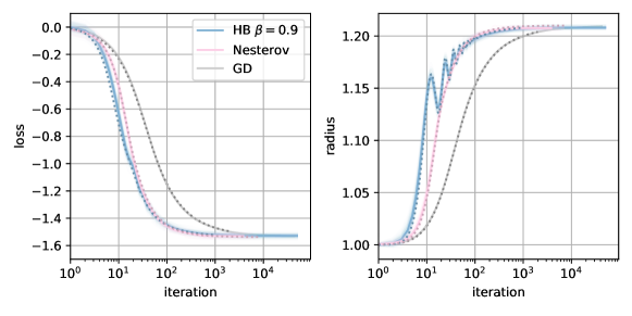
Figure 1: Simulation and DMFT comparison in mixed $p$-spin model. The simulations in the figures have parameters $p=3$, $\Delta_{3}=2/p$, $\Delta_{2}=1$, ridge parameter $\mu=10$ and input dimension $N=1024$. In all our simulations we use the dilution technique Semerjian et al. (2004); Krzakala and Zdeborová (2013) to reduce the computational cost. We consider: Nesterov acceleration in pink; heavy ball momentum in blue with $\alpha=0.01$ and $\beta=0.9$; and gradient descent in grey. We run 100 simulations (in transparency) and draw the average. The parameters for heavy ball are the best parameters found in our simulations, see also Fig. 2 for a comparison. The results from the DMFT equations are drawn with dotted lines.

We use dynamical mean field theory (DMFT) techniques to derive a set of equation describing the evolution of the algorithms in the high-dimensional limit. The method has its origin in statistical physics and can be applied to the study of Langevin dynamics of disordered systems Martin et al. (1973); De Dominicis (1978); Mézard et al. (1987). More recently it was proved to be rigorous in the case of the mixed $p$-spin model Ben Arous et al. (2006); Dembo and Subag (2020). The application to the inference version of the optimization problem is in Sarao Mannelli et al. (2020b, 2019b). The same techniques have also been applied to study the stochastic gradient descent dynamics in single layer networks Mignacco et al. (2020) and in the analysis of recurrent neural networks Sompolinsky et al. (1988); Mastrogiuseppe and Ostojic (2017); Can et al. (2020).

The derivation presented in the rest of the section is heuristic and, as such, it is not fully rigorous. Making our results rigorous would be an extension of the works Ben Arous et al. (2006); Dembo and Subag (2020) where path-integral methods are used to prove a large deviation principle for the infinite-dimensional limit. Our non-rigorous results are checked against extensive numerical simulations.

The idea behind DMFT is that, if the input dimension $N$ is sufficiently large, one can obtain a description of the dynamics in terms of the typical evolution of a representative entry of the vector $\boldsymbol{x}$ (and vector $\boldsymbol{y}$ when it applies). The representative element evolves according to a non-Markovian stochastic process whose memory term and noise source encode, in a self-consistent way, the interaction with all the other components of vector $\boldsymbol{x}$ (and $\boldsymbol{y}$). The memory terms as well as the statistical properties of the noise are described by dynamical order parameters which, in the present model, are given by the dynamical two-time correlation and response functions.

In this first step of the analysis we obtain an effective dynamics for a representative entry $x_{i}$ (and $y_{i}$). The next step consists in using such equations to compute self-consistently the properties of the corresponding stochastic processes, namely the memory kernel and the statistical correlation of the noise. In Fig. 1 we anticipate the results by comparing numerical simulations with the integration of the DMFT equations for the different algorithms: on the left we observe the evolution of the loss, on the right we observe the evolution of the radius of the vector $\boldsymbol{x}$, defined as the $L_{2}$ norm of the vector $||\boldsymbol{x}||_{2}$. We find a good agreement between the DMFT state evolution and the numerical simulations.

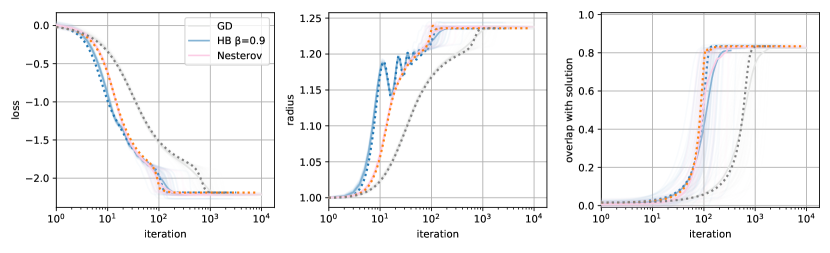
Figure 3: DMFT in the spiked matrix-tensor model. Performance of heavy ball and Nesterov in the spiked matrix-tensor model with $p=3$, $1/\Delta_{2}=2.7$, $\Delta_{3}=1.0$, and $\mu=10$. The parameters in the simulations are: $\alpha=0.01$ and $\beta=0.9$ for HB. The different solid lines correspond to simulations with input dimension $N=8192$, while the dotted lines are obtained from the DMFT that, by definition, is in the infinite dimension limit. In the spiked version of the model the finite size effects are stronger and larger simulation sizes are needed.

We compare Nesterov acceleration with the heavy ball momentum in the mixed $p$-spin model Fig. 1, and in the spiked model Fig. 3. Nesterov acceleration allows for a fast convergence to the asymptotic energy without need of parameter tuning. In Fig. 2 we compare the numerical simulations for the HB algorithm and the DMFT description of the corresponding massive momentum version for several control parameters.

DMFT equations

In the following we describe the resulting DMFT equations for the correlation and response functions. The details of their derivation for the case of the Nesterov acceleration are provided in the following section, while we leave the other cases to the supplementary material (SM). The dynamical order parameters appearing in the DMFT equations are one-time or two-time correlations, e.g. $C_{xy}[t,t^{\prime}]=\sum_{i}x_{i}[t]y_{i}[t^{\prime}]/N$, and response to instantaneous perturbation of the dynamics, e.g. $R_{x}[t,t^{\prime}]=\big{(}\sum_{i}\delta x_{i}[t]/\delta H_{i}[t^{\prime}]\big{)}/N$ by a local field $\boldsymbol{H}[t^{\prime}]\in\mathbb{R}^{N}$ where the symbol $\delta$ denotes the functional derivative. In this section we show only the equations for the mixed $p$-spin model and we discuss the difference and the derivation of the equations for the spiked tensor in the SM.

From the order parameters we can evaluate useful quantities that describe the evolution of the algorithms. In particular in Figs. 1,2,3 we show the loss, the radius, and the overlap with the solution in the spiked case (Fig. 3):

• Average loss

  $$\begin{split}&\mathcal{L}[t]=-\frac{\alpha}{\Delta_{p}C_{x}[t,t]^{\frac{p}{2}}}\sum\limits_{t^{\prime\prime}=0}^{t}R_{x}[t,t^{\prime}]C_{x}[t,t^{\prime}]^{p-1}-\frac{\alpha}{\Delta_{2}C_{x}[t,t]}\sum\limits_{t^{\prime\prime}=0}^{t}R_{x}[t,t^{\prime}]C_{x}[t,t^{\prime}];\end{split}$$ (8)

• Radius $\sqrt{C_{x}[t,t]}$;

• Define $m_{x}[t]=\frac{1}{N}\sum_{i}x_{i}[t]x_{i}^{*}$ an additional order parameter for the spiked matrix-tensor model (more details are given in the SM), the overlap with ground truth is

  $$\frac{\boldsymbol{x}[t]\cdot\boldsymbol{x}^{*}}{{||\boldsymbol{x}||}}=\frac{m_{x}[t]}{\sqrt{C_{x}[t,t]}}$$

Nesterov acceleration.

It has been shown that this algorithm has a quadratic convergence rate to the minimum in convex optimization problems under Lipschitz loss functions Nesterov (1983); Su et al. (2014), thus it outperforms standard gradient descent whose convergence is linear in the number of iterations. The analysis of the algorithm is described by the flow of the following dynamical correlation functions

$$C_{x}[t,t^{\prime}]=\frac{1}{N}\sum_{i}x_{i}[t]x_{i}[t^{\prime}],$$ (9)

$$C_{y}[t,t^{\prime}]=\frac{1}{N}\sum_{i}y_{i}[t]y_{i}[t^{\prime}],$$ (10)

$$C_{xy}[t,t^{\prime}]=\frac{1}{N}\sum_{i}x_{i}[t]y_{i}[t^{\prime}],$$ (11)

$$R_{x}[t,t^{\prime}]=\frac{1}{N}\sum_{i}\frac{\delta x_{i}[t]}{\delta H_{i}[t^{\prime}]},$$ (12)

$$R_{y}[t,t^{\prime}]=\frac{1}{N}\sum_{i}\frac{\delta y_{i}[t]}{\delta H_{i}[t^{\prime}]}.$$ (13)

The dynamical equations are obtained following the procedure detailed in section 4. Call $Q(x)=x^{2}/(2\Delta_{2})+x^{p}/(p\Delta_{p})$,

$$\begin{split}&C_{x}[t+1,t^{\prime}]=C_{xy}[t,t^{\prime}]-\alpha\mu\left(C_{y}[t,t]-1\right)C_{y}[t,t^{\prime}]+\alpha^{2}\sum_{t^{\prime\prime}=0}^{t^{\prime}}R_{x}[t^{\prime},t^{\prime\prime}]Q^{\prime}\left(C_{y}[t,t^{\prime\prime}]\right)+\\ &\quad\quad+\alpha^{2}\sum_{t^{\prime\prime}=0}^{t}R_{y}[t,t^{\prime\prime}]Q^{\prime\prime}\left(C_{y}[t,t^{\prime\prime}]\right)C_{xy}[t^{\prime},t^{\prime\prime}];\end{split}$$ (14)

$$\begin{split}&C_{xy}[t+1,t^{\prime}]=C_{y}[t,t^{\prime}]-\alpha\mu\left(C_{y}[t,t]-1\right)C_{xy}[t,t^{\prime}]+\alpha^{2}\sum_{t^{\prime\prime}=0}^{t^{\prime}}R_{y}[t^{\prime},t^{\prime\prime}]Q^{\prime}\left(C_{y}[t,t^{\prime\prime}]\right)+\\ &\quad\quad+\alpha^{2}\sum_{t^{\prime\prime}=0}^{t}R_{y}[t,t^{\prime\prime}]Q^{\prime\prime}\left(C_{y}[t,t^{\prime\prime}]\right)C_{y}[t^{\prime},t^{\prime\prime}];\end{split}$$ (15)

$$C_{xy}[t^{\prime},t+1]=\frac{2t+3}{t+3}C_{x}[t+1,t^{\prime}]-\frac{t}{t+3}C_{x}[t,t^{\prime}];$$ (16)

$$C_{y}[t^{\prime},t+1]=\frac{2t+3}{t+3}C_{xy}[t+1,t^{\prime}]-\frac{t}{t+3}C_{xy}[t,t^{\prime}];$$ (17)

$$\begin{split}&R_{x}[t+1,t^{\prime}]=R_{y}[t,t^{\prime}]+\delta_{t,t^{\prime}}-\alpha\mu\left(C_{y}[t,t]-1\right)R_{y}[t,t^{\prime}]\\ &\quad\quad+\alpha^{2}\sum_{t^{\prime\prime}=t^{\prime}}^{t}R_{y}[t,t^{\prime\prime}]R_{y}[t^{\prime\prime},t^{\prime}]Q^{\prime\prime}\left(C_{y}[t,t^{\prime\prime}]\right);\end{split}$$ (18)

$$R_{y}[t^{\prime},t+1]=\frac{2t+3}{t+3}R_{x}[t+1,t^{\prime}]-\frac{t}{t+3}R_{x}[t,t^{\prime}].$$ (19)

The initial conditions are: $C_{x}[0,0]=1$, $C_{y}[0,0]=1$, $C_{xy}[0,0]=1$, $R_{x}[t+1,t]=1$, $R_{y}[t+1,t]=\frac{2t+3}{t+3}$.

The equations show a discretized version of the typical structure of DMFT equations. We can observe: terms immediately ascribable to the dynamical equations (3,4) and summations whose interpretation is less trivial without looking into the derivation. They represent memory kernels that take into account linear response theory for small perturbations to the dynamics (e.g. the last term of Eq. equation 14) and a noise whose statistical properties encode the effect of all the degrees of freedom on a representative one (e.g. the second last term of Eq. equation 14).

Heavy ball momentum.

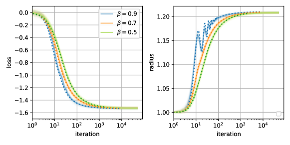
Figure 2: DMFT for HB. Simulations of HB momentum in the mixed $p$-spin model with $p=3$, $\Delta_{3}=2/p$, $\Delta_{2}=1$, ridge parameter $\mu=10$ and input dimension $N=1024$. The parameters are $\alpha=0.01$ for all the simulations and $\beta\in\{0.5,0.7,0.9\}$. We use solid lines to represent the result from the simulation, the dotted lines for the DMFT of HB.

The DMFT equations are obtained analogously to previous ones,

$$\begin{split}&C_{y}[t+1,t^{\prime}]=\beta C_{y}[t,t^{\prime}]+\mu\left(C_{x}[t,t]-1\right)C_{xy}[t,t^{\prime}]+\alpha\sum_{t^{\prime\prime}=0}^{t^{\prime}}R_{y}[t^{\prime},t^{\prime\prime}]Q^{\prime}\left(C_{x}[t,t^{\prime\prime}]\right)\\ &\quad\quad+\alpha\sum_{t^{\prime\prime}=0}^{t}R_{x}[t,t^{\prime\prime}]Q^{\prime\prime}\left(C_{x}[t,t^{\prime\prime}]\right)C_{xy}[t^{\prime\prime},t^{\prime}];\end{split}$$ (20)

$$\begin{split}&C_{xy}[t^{\prime},t+1]=\beta C_{xy}[t^{\prime},t]+\mu\left(C_{x}[t,t]-1\right)C_{x}[t,t^{\prime}]+\alpha\sum_{t^{\prime\prime}=0}^{t^{\prime}}R_{x}[t^{\prime},t^{\prime\prime}]Q^{\prime}\left(C_{x}[t,t^{\prime\prime}]\right)\\ &\quad\quad+\alpha\sum_{t^{\prime\prime}=0}^{t}R_{x}[t,t^{\prime\prime}]Q^{\prime\prime}\left(C_{x}[t,t^{\prime\prime}]\right)C_{x}[t^{\prime},t^{\prime\prime}];\end{split}$$ (21)

$$C_{xy}[t+1,t^{\prime}]=C_{xy}[t,t^{\prime}]-\alpha C_{y}[t+1,t^{\prime}];$$ (22)

$$C_{x}[t+1,t^{\prime}]=C_{x}[t,t^{\prime}]-\alpha C_{xy}[t^{\prime},t+1];$$ (23)

$$\begin{split}&R_{y}[t+1,t^{\prime}]=\beta R_{y}[t,t^{\prime}]+\frac{1}{\alpha}\delta_{t,t^{\prime}}+\mu\left(C_{x}[t,t]-1\right)R_{x}[t,t^{\prime}]\\ &\quad\quad+\alpha\sum_{t^{\prime\prime}=0}^{t}R_{x}[t,t^{\prime\prime}]R_{x}[t^{\prime\prime},t^{\prime}]Q^{\prime\prime}\left(C_{x}[t,t^{\prime\prime}]\right);\end{split}$$ (24)

$$R_{x}[t+1,t^{\prime}]=R_{x}[t,t^{\prime}]-\alpha R_{y}[t+1,t^{\prime}].$$ (25)

with initial conditions: $C_{x}[0,0]=1$, $C_{y}[0,0]=0$, $C_{xy}[0,0]=0$, $R_{y}[t+1,t]=1/\alpha$, $R_{x}[t+1,t]=-1$. Fig. 2 shows the consistency of theory and simulations.

Mappings between discrete update equation and continuous flow for both heavy ball momentum and Nesterov acceleration have been proposed in the literature. In the SM we considered the work Qian (1999) that maps HB to second order ODEs in some regimes of $\alpha$ and $\beta$. This mapping establishes the equivalence of the algorithm to the physics problem of a massive particle moving under the action of a potential. This problem has been studied in Cugliandolo et al. (2017) but the result is limited to the fully under-damped regime where there is no first order derivative term, corresponding therefore to a dynamics that is fully inertial and which never stops due to energy conservation. In the SM we obtain the dynamical equations for arbitrary damping regimes, and we recover the equivalence established in Qian (1999) comparing the results from the two DMFTs formulations.

Gradient descent.

A simple way to obtain the gradient descent DMFT is by taking the limit $m\rightarrow 0$ in the DMFT of the massive momentum description of HB. We get

$$\begin{split}&C_{x}[t+1,t^{\prime}]=C_{x}[t,t^{\prime}]-\alpha\mu\left(C_{x}[t,t]-1\right)C_{x}[t,t^{\prime}]+\alpha^{2}\sum_{t^{\prime\prime}=0}^{t^{\prime}}R_{x}[t^{\prime},t^{\prime\prime}]Q^{\prime}\left(C_{x}[t,t^{\prime\prime}]\right)\\ &\quad\quad+\alpha^{2}\sum_{t^{\prime\prime}=0}^{t}R_{x}[t,t^{\prime\prime}]Q^{\prime\prime}\left(C_{x}[t,t^{\prime\prime}]\right)C_{x}[t^{\prime},t^{\prime\prime}];\end{split}$$ (26)

$$\begin{split}&R_{x}[t+1,t^{\prime}]=R_{x}[t,t^{\prime}]+\delta_{t,t^{\prime}}+\alpha^{2}\sum_{t^{\prime\prime}=0}^{t}R_{x}[t,t^{\prime\prime}]R_{x}[t^{\prime\prime},t^{\prime}]Q^{\prime\prime}\left(C_{x}[t,t^{\prime\prime}]\right)\\ &\quad\quad-\alpha\mu\left(C_{x}[t,t]-1\right)R_{x}[t,t^{\prime}].\end{split}$$ (27)

with initial conditions: $C_{x}[0,0]=1$, and $R_{x}[t+1,t]=1$. Apart from the $\mu$-dependent term, these equations are a particular case of the ones that appear in Cugliandolo and Kurchan (1993); Crisanti et al. (1993) and we point to these previous references for details.

4 Derivation of DMFT for Nesterov acceleration

The approach for the DMFT proposed in this section is based on the dynamical cavity method Mézard et al. (1987). Consider the problem having dimension $N+1$ and denote the additional entry of the vectors $\boldsymbol{x}$ and $\boldsymbol{y}$ with the subscript $0$, $x_{0}$ and $y_{0}$. The idea behind cavity method is to evaluate how this additional dimension changes the dynamics of all degrees of freedom. If the dimension is sufficiently large the dynamics is only slightly modified by the additional dimension, and the effect of the additional degree of freedom can be tracked in perturbation theory.

The framework described in this section might be extended to more other momentum-based algorithms (such as PID An et al. (2018) and quasi-hyperbolic momentum Ma and Yarats (2019)) with some minor adaptations. The steps to follow Mézard et al. (1987) can be summarised in:

• Writing the equation of motion isolating the contributions of an additional degree of freedom, leading to Eqs. (28-30;

• Treating the effect of the terms containing the new degree of freedom in perturbation theory, Eqs. (32-34);

• Identifying the order dynamical order parameters, namely dynamical correlation and response functions, Eqs. (37,38).

Consider the Nesterov update algorithm and isolate the effect of the additional degree of freedom

$$x_{i}[t+1]=y_{i}[t]+\alpha\sum_{j\neq 0}J_{ij}y_{j}[t]+\alpha\sum_{(i,i_{2},\dots,i_{p})}J_{i,i_{2},\dots,i_{p}}y_{i_{2}}[t]\dots y_{i_{p}}[t]-\alpha\mu\left(\sum_{j\neq 0}\frac{y_{j}^{2}[t]}{N}-1\right)y_{i}[t]$$ (28)

$$\quad\quad+\alpha\sum_{(i,0,i_{3},\dots,i_{p})}J_{i,0,i_{3},\dots,i_{p}}y_{0}[t]y_{i_{3}}[t]\dots y_{i_{p}}[t]+\alpha J_{i0}y_{0}[t]+\frac{\mu}{N}y_{0}^{2}[t]y_{i}[t],$$ (29)

$$y_{i}[t+1]=x_{i}[t+1]+\frac{t}{t+3}\left(x_{i}[t+1]-x_{i}[t]\right).$$ (30)

We identify the term in line (29) as a perturbation, denoted by $H_{i}[t]$. We will assume that the perturbation is sufficiently small and the effective dynamics is well approximated by a first order expansion around the original updates, so-called linear response regime. Therefore, the perturbed entries can be written as

$$x_{i}[t]\approx x_{i}^{0}+\alpha\sum_{t^{\prime\prime}=0}^{t}\frac{\delta x_{i}[t]}{\delta H_{i}[t^{\prime\prime}]}H_{i}[t^{\prime\prime}],\quad\quad y_{i}[t]\approx y_{i}^{0}+\alpha\sum_{t^{\prime\prime}=0}^{t}\frac{\delta y_{i}[t]}{\delta H_{i}[t^{\prime\prime}]}H_{i}[t^{\prime\prime}].$$ (31)

The dynamics of the 0th degree of freedom to the leading order in the perturbation is

$$x_{0}[t+1]=y_{0}[t]-\alpha\mu\Big{(}\frac{1}{N}\sum_{j}y_{j}^{2}[t]-1\Big{)}y_{0}[t]+\Xi[t]+\alpha^{2}\sum_{j}J_{0j}\sum_{t^{\prime\prime}=0}^{t}\frac{\delta y_{j}[t]}{\delta H_{j}[t^{\prime\prime}]}H_{j}[t^{\prime\prime}]$$ (32)

$$\quad+\alpha^{2}\sum_{(0,i_{2},\dots,i_{p})}J_{0,i_{2},\dots,i_{p}}\Big{(}\sum_{t^{\prime\prime}=0}^{t}\frac{\delta y_{i_{2}}[t]}{\delta H_{i_{2}}[t^{\prime\prime}]}H_{i_{2}}[t^{\prime\prime}]y_{i_{3}}[t]\dots y_{i_{p}}[t]+\text{perm.}\Big{)}+\mathcal{O}\Big{(}\frac{1}{N}\Big{)},$$ (33)

$$y_{i}[t+1]=x_{i}[t+1]+\frac{t}{t+3}\left(x_{i}[t+1]-x_{i}[t]\right),$$ (34)

with $\Xi=\alpha\sum_{j}J_{0j}y_{j}[t]+\alpha\sum_{(0,i_{2},\dots,i_{p})}J_{0,i_{2},\dots,i_{p}}y_{i_{2}}[t]\dots y_{i_{p}}[t]$ a Gaussian noise with moments:

$$\mathbb{E}[\Xi[t]]=0,$$

$$\mathbb{E}[\Xi[t]\Xi[t^{\prime}]]=\frac{1}{\Delta_{2}}C_{y}[t,t^{\prime}]+\frac{1}{\Delta_{p}}C_{y}^{p-1}[t,t^{\prime}]=Q^{\prime}\left(C_{y}[t,t^{\prime}]\right)\dot{=}\mathbb{K}[t,t^{\prime}].$$

The terms in Eqs. (32,33) can be simplified. Consider the last term in Eq. equation 32: after substituting the $H_{i}$, $J_{0j}J_{0j}$ and $J_{0j}J_{(j,0,\dots,i_{p})}$ can be approximated by their expected values with a difference that is subleading in $1/N$

$$\alpha^{2}\sum_{j}J_{0j}\sum_{t^{\prime\prime}=0}^{t}\frac{\delta y_{j}[t]}{\delta H_{j}[t^{\prime\prime}]}J_{0j}y_{0}[t^{\prime\prime}]\approx\frac{\alpha^{2}}{\Delta_{2}N}\sum_{t^{\prime\prime}=0}^{t}\frac{\delta y_{j}[t]}{\delta H_{j}[t^{\prime\prime}]}y_{0}[t^{\prime\prime}]=\frac{\alpha^{2}}{\Delta_{2}}\sum_{t^{\prime\prime}=0}^{t}R_{y}[t,t^{\prime\prime}]y_{0}[t^{\prime\prime}],$$ (35)

where the last equality follows from the definition of response function in $y$.
The same approximation is applied to Eq. (33), taking carefully into account the permutations, obtaining

$$\frac{\alpha^{2}(p-1)}{\Delta_{p}}\sum_{t^{\prime\prime}=0}^{t}R_{y}[t,t^{\prime\prime}]\left(C_{y}[t,t^{\prime\prime}]\right)^{p-2}y_{0}[t^{\prime\prime}].$$ (36)

Finally, collecting all terms, the effective dynamics of the additional dimension is given by

$$\begin{split}&x_{0}[t+1]=y_{0}[t]+\alpha\Xi[t]-\alpha\mu\left(C_{y}[t,t]-1\right)y_{0}[t]+\alpha^{2}\sum_{t^{\prime\prime}=0}^{t}R_{y}[t,t^{\prime\prime}]Q^{\prime\prime}\left(C_{y}[t,t^{\prime\prime}]\right)y_{0}[t^{\prime\prime}];\end{split}$$ (37)

$$y_{0}[t+1]=x_{0}[t+1]+\frac{t}{t+3}\left(x_{0}[t+1]-x_{0}[t]\right).$$ (38)

In order to derive the updates of the order parameters, we need the expected values of $\langle\Xi[t]x_{0}[t^{\prime}]\rangle$ and $\langle\Xi[t]y_{0}[t^{\prime}]\rangle$ with respect to the stochastic process. These are obtained using Girsanov theorem

$$\begin{split}\langle\Xi[t]x_{0}[t^{\prime}]\rangle&=\alpha\sum_{t^{\prime\prime}}R_{x}[t^{\prime},t^{\prime\prime}]Q^{\prime}\left(C_{y}[t,t^{\prime\prime}]\right),\quad\quad\langle\Xi[t]y_{0}[t^{\prime}]\rangle=\alpha\sum_{t^{\prime\prime}}R_{y}[t^{\prime},t^{\prime\prime}]Q^{\prime}\left(C_{y}[t,t^{\prime\prime}]\right).\end{split}$$

The final step consists in substituting the Eqs. (37,38) into the equations of the order parameters Eqs. (14-19). Then we identify the order parameters in the equations and use the results of Girsanov theorem to obtain the dynamical equations reported in section 3.

5 Algorithmic threshold

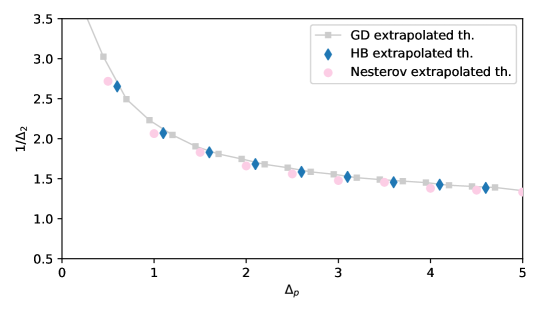
Figure 4: Phase diagram of the spiked matrix-tensor model. The horizontal and vertical axis represent the parameters of the model $\Delta_{p}$ and $1/\Delta_{2}$. We identify two regions in the diagram: where Nesterov, heavy ball and gradient descent algorithms lead to the hidden solution (upper region), and where they fail (lower region). The grey square connected by a solid line represents the threshold of gradient descent estimated numerically as detailed in the text. We use points to indicate the threshold extrapolated from the DMFT: pink circles for Nesterov acceleration and blue diamonds for heavy ball momentum with $\beta=0.9$ and $\alpha=0.01$.

Finally we investigate the performance of accelerated methods in recovering a signal in a complex non-convex landscape. The dynamics of the gradient descent has been studied in the spiked matrix-tensor model in Sarao Mannelli et al. (2019b). Using DMFT it was possible to compute the phase diagram for signal recovery in terms of the noise levels $\Delta_{2}$ and $\Delta_{p}$. This phase diagram was later confirmed theoretically Sarao Mannelli et al. (2019a).

Given the DMFT equations derived in the previous sections we can apply the analysis used in Sarao Mannelli et al. (2019b) to accelerated gradient methods. Given order of the tensor $p$ and $\Delta_{p}$, increasing $\Delta_{2}$ the problem becomes harder and moves from the easy phase - where the signal can be partially recovered - to an algorithmically impossible phase - where the algorithm remains stuck at vanishingly small overlap with the signal. The goal of the analysis is to characterize the algorithmic threshold that separates the two phases. Using the DMFT we estimate the relaxation time – the time the accelerated methods need to find the signal. Since this time diverges approaching the algorithmic threshold, the fit of the divergence point gives an estimation of the threshold.

More precisely, for each value of $\Delta_{p}$ as the noise to signal ratio ($\Delta_{2}$) increases the simulation time required to arrive close to the signal increases like a power law $\sim a\ |\Delta_{2}-\Delta_{2}^{al.}(\Delta_{p})|^{-\theta}$. The algorithmic threshold $\Delta_{2}^{al.}(\Delta_{p})$ is obtained by fitting the parameters of the power law $(a,\theta,\Delta_{2}^{al.})$. In the SM we show an example of the extrapolation of a single point where many initial conditions $m_{x}(0)$ are considered in order to correctly characterize the limits $N\rightarrow\infty$ and $m_{x}(0)\rightarrow 0^{+}$. Finally the fits obtained for the three algorithms and for several $\Delta_{p}$ are shown in the phase diagram of Fig. 4 for $p=3$. We observe that all the algorithms give very close thresholds. DMFT allows to obtain a good estimation of the threshold, free from finite size effects and stochastic fluctuations that are present in the direct estimation from the simulations.

Conclusions and broader impact

In this work we analysed momentum-accelerated methods in two paradigmatic high-dimensional non-convex problems: the mixed $p$-spin model and the spiked matrix-tensor model. Our analysis is based on dynamical mean field theory and provides a set of equations that characterize the average evolution of the dynamics. We have focused on Polyak’s heavy ball and Nesterov acceleration, but the same techniques may be applied to more recent methods such as quasi-hyperbolic momentum Ma and Yarats (2019) and proportional integral-derivative control algorithm An et al. (2018).

Momentum-based methods are techniques commonly used in practice but poorly understood at the theoretical level. This work analysed the dynamics of momentum-based algorithms in a very controlled setting of a high-dimensional non-convex inference problem which allowed us to establish that accelerated methods have a recovery threshold which is – within the limits of numerical integration – the same of vanilla gradient descent.

Our analysis can be easily extended to 1-layer neural networks – combining our technical results with the techniques of Mignacco et al. (2020) – and to simple inference problem seen from the learning point of view, such as the phase retrieval problem Mignacco et al. (2021). The same questions can also be analysed in the context of recurrent networks Mastrogiuseppe and Ostojic (2017); Can et al. (2020) where DMFT approaches have already been applied to gradient-based methods.

Our study is theoretical in nature and we do not foresee any societal impact.

 

Supplemental Material

 

Appendix A Spiked matrix-tensor model

In this section we discuss how the DMFT equations of the spiked matrix-tensor model differ from the mixed $p$-spin model. The main difference is that the hidden solution deforms locally the loss function

$$\begin{split}\mathcal{H}&=-\frac{1}{\Delta_{p}}\sqrt{\frac{(p-1)!}{N^{p-1}}}\sum_{i_{1},\dots,i_{p}=1}^{N}T_{i_{1},\dots,i_{p}}x_{i_{1}}\dots x_{i_{p}}-\frac{1}{\Delta_{2}}\frac{1}{\sqrt{N}}\sum_{i,j=1}^{N}Y_{ij}x_{i}x_{j}+\\ &-\frac{1}{p\Delta_{p}}\left(\frac{1}{N}\sum_{j}x_{j}x_{j}^{*}\right)^{p}-\frac{1}{2\Delta_{2}}\left(\frac{1}{N}\sum_{j}x_{j}x_{j}^{*}\right)^{2}+\frac{\mu}{4N}\left(\sum_{i=1}^{N}x_{i}^{2}-N\right)^{2}.\end{split}$$ (39)

As it clearly appears from the equation of the loss, the overlap of the hidden solution with the estimator plays an important role. This leads to two additional order parameters $m_{x}[t]=\frac{1}{N}\sum_{j}x_{j}[t]x_{j}^{*}$ and $m_{y}[t]=\frac{1}{N}\sum_{j}y_{j}[t]x_{j}^{*}$ (or $m_{v}(t)=\frac{1}{N}\sum_{j}v_{j}(t)x_{j}^{*}$ for massive gradient flow).

Since the stochastic part of the loss is unchanged, the derivation follows same steps shown in section 4 of the main text. They lead to modified dynamical equations where overlap with the hidden solution is present, for instance in Nesterov they are

$$\begin{split}&x_{0}[t+1]=y_{0}[t]+\alpha\Xi[t]-\alpha\mu\left(C_{y}[t,t]-1\right)y_{0}[t]+\\ &\quad\quad+\alpha^{2}\sum_{t^{\prime\prime}=0}^{t}R_{y}[t,t^{\prime\prime}]Q^{\prime\prime}\left(C_{y}[t,t^{\prime\prime}]\right)y_{0}[t^{\prime\prime}]+Q^{\prime}(m_{y}[t])\boldsymbol{x}^{*},\end{split}$$ (40)

$$y_{0}[t+1]=x_{0}[t+1]+\frac{t}{t+3}\left(x_{0}[t+1]-x_{0}[t]\right).$$ (41)

Finally, substituting the effective dynamics into the definition of the order parameters we obtain:

• for Nesterov acceleration

  $$\begin{split}&C_{x}[t+1,t^{\prime}]=C_{xy}[t,t^{\prime}]+\alpha^{2}\sum_{t^{\prime\prime}=0}^{t^{\prime}}R_{x}[t^{\prime},t^{\prime\prime}]Q^{\prime}\left(C_{y}[t,t^{\prime\prime}]\right)+\alpha^{2}\sum_{t^{\prime\prime}=0}^{t}R_{y}[t,t^{\prime\prime}]Q^{\prime\prime}\left(C_{y}[t,t^{\prime\prime}]\right)C_{xy}[t^{\prime},t^{\prime\prime}]+\\ &\quad\quad-\alpha\mu\left(C_{y}[t,t]-1\right)C_{y}[t,t^{\prime}]-Q^{\prime}(m_{y}[t])m_{x}[t^{\prime}],\end{split}$$

  $$\begin{split}&C_{xy}[t+1,t^{\prime}]=C_{y}[t,t^{\prime}]+\alpha^{2}\sum_{t^{\prime\prime}=0}^{t^{\prime}}R_{y}[t^{\prime},t^{\prime\prime}]Q^{\prime}\left(C_{y}[t,t^{\prime\prime}]\right)+\alpha^{2}\sum_{t^{\prime\prime}=0}^{t}R_{y}[t,t^{\prime\prime}]Q^{\prime\prime}\left(C_{y}[t,t^{\prime\prime}]\right)C_{y}[t^{\prime},t^{\prime\prime}]+\\ &\quad\quad-\alpha\mu\left(C_{y}[t,t]-1\right)C_{xy}[t,t^{\prime}]-Q^{\prime}(m_{y}[t])m_{y}[t^{\prime}],\end{split}$$

  $$C_{xy}[t^{\prime},t+1]=C_{x}[t+1,t^{\prime}]+\frac{t}{t+3}\left(C_{x}[t+1,t^{\prime}]-C_{x}[t,t^{\prime}]\right),$$

  $$C_{y}[t^{\prime},t+1]=C_{xy}[t+1,t^{\prime}]+\frac{t}{t+3}\left(C_{xy}[t+1,t^{\prime}]-C_{xy}[t,t^{\prime}]\right),$$

  $$R_{x}[t+1,t^{\prime}]=R_{y}[t,t^{\prime}]+\delta_{t,t^{\prime}}+\alpha^{2}\sum_{t^{\prime\prime}=t^{\prime}}^{t}R_{y}[t,t^{\prime\prime}]R_{y}[t^{\prime\prime},t^{\prime}]Q^{\prime\prime}\left(C_{y}[t,t^{\prime\prime}]\right)-\alpha\mu\left(C_{y}[t,t]-1\right)R_{y}[t,t^{\prime}],$$

  $$R_{y}[t^{\prime},t+1]=R_{x}[t+1,t^{\prime}]+\frac{t}{t+3}\left(R_{x}[t+1,t^{\prime}]-R_{x}[t,t^{\prime}]\right),$$

  $$m_{x}[t+1]=m_{y}[t]-\alpha\mu\left(C_{y}[t,t]-1\right)m_{y}[t]+\alpha^{2}\sum_{t^{\prime\prime}=0}^{t}R_{y}[t,t^{\prime\prime}]Q^{\prime\prime}\left(C_{y}[t,t^{\prime\prime})\right)m_{y}[t^{\prime\prime}]+Q^{\prime}\left(m_{y}[t]\right),$$

  $$m_{y}[t+1]=m_{x}[t+1]+\frac{t}{t+3}\left(m_{x}[t+1]-m_{x}[t]\right),$$

  with initial conditions $C_{x}[0,0]=1$, $C_{y}[0,0]=1$, $C_{xy}[0,0]=1$, $R_{x}[t+1,t]=1$, $R_{y}[t+1,t]=\frac{2t+3}{t+3}$, $m_{x}[0]=0^{+}$, $m_{y}[0]=0^{+}$;

• for heavy ball momentum.

  $$\begin{split}&C_{y}[t+1,t^{\prime}]=\beta C_{y}[t,t^{\prime}]+\mu\left(C_{x}[t,t]-1\right)C_{xy}[t,t^{\prime}]+\alpha\sum_{t^{\prime\prime}=0}^{t^{\prime}}R_{y}[t^{\prime},t^{\prime\prime}]Q^{\prime}\left(C_{x}[t,t^{\prime\prime}]\right)\\ &\quad\quad+\alpha\sum_{t^{\prime\prime}=0}^{t}R_{x}[t,t^{\prime\prime}]Q^{\prime\prime}\left(C_{x}[t,t^{\prime\prime}]\right)C_{xy}[t^{\prime\prime},t^{\prime}]-Q^{\prime}(m_{x}[t])m_{y}[t^{\prime}];\end{split}$$

  $$\begin{split}&C_{xy}[t^{\prime},t+1]=\beta C_{xy}[t^{\prime},t]+\mu\left(C_{x}[t,t]-1\right)C_{x}[t,t^{\prime}]+\alpha\sum_{t^{\prime\prime}=0}^{t^{\prime}}R_{x}[t^{\prime},t^{\prime\prime}]Q^{\prime}\left(C_{x}[t,t^{\prime\prime}]\right)\\ &\quad\quad+\alpha\sum_{t^{\prime\prime}=0}^{t}R_{x}[t,t^{\prime\prime}]Q^{\prime\prime}\left(C_{x}[t,t^{\prime\prime}]\right)C_{x}[t^{\prime},t^{\prime\prime}]-Q^{\prime}(m_{x}[t])m_{x}[t^{\prime}];\end{split}$$

  $$C_{xy}[t+1,t^{\prime}]=C_{xy}[t,t^{\prime}]-\alpha C_{y}[t+1,t^{\prime}];$$

  $$C_{x}[t+1,t^{\prime}]=C_{x}[t,t^{\prime}]-\alpha C_{xy}[t^{\prime},t+1];$$

  $$\begin{split}&R_{y}[t+1,t^{\prime}]=\beta R_{y}[t,t^{\prime}]+\frac{1}{\alpha}\delta_{t,t^{\prime}}+\mu\left(C_{x}[t,t]-1\right)R_{x}[t,t^{\prime}]\\ &\quad\quad+\alpha\sum_{t^{\prime\prime}=0}^{t}R_{x}[t,t^{\prime\prime}]R_{x}[t^{\prime\prime},t^{\prime}]Q^{\prime\prime}\left(C_{x}[t,t^{\prime\prime}]\right);\end{split}$$

  $$R_{x}[t+1,t^{\prime}]=R_{x}[t,t^{\prime}]-\alpha R_{y}[t+1,t^{\prime}]$$

  $$\begin{split}&m_{y}[t+1]=\beta m_{y}[t]-\mu\left(C_{x}[t,t]-1\right)m_{x}[t]+\\ &\quad\quad+\sum_{t^{\prime\prime}=0}^{t}R_{x}[t,t^{\prime\prime}]Q^{\prime\prime}\left(C_{x}[t,t^{\prime\prime})\right)m_{x}[t^{\prime\prime}]-Q^{\prime}\left(m_{x}[t]\right),\end{split}$$

  $$m_{x}[t+1]=m_{x}[t]-\alpha m_{y}[t+1].$$

  with initial conditions: $C_{x}[0,0]=1$, $C_{y}[0,0]=0$, $C_{xy}[0,0]=0$, $R_{y}[t+1,t]=1/\alpha$, $R_{x}[t+1,t]=-1$, $m_{y}[0]=O^{+}$, $m_{x}[0]=O^{+}$.

• for massive gradient flow (see Sec. C)

  $$\partial_{t}C_{x}(t,t^{\prime})=C_{xv}(t^{\prime},t)\ ,$$

  $$\begin{split}&m\partial_{t}C_{v}(t,t^{\prime})=-C_{v}(t,t^{\prime})+\int_{0}^{t}dt^{\prime\prime}R_{x|v}(t,t^{\prime\prime})Q^{\prime\prime}[C_{x}(t,t^{\prime\prime})]C_{xv}(t^{\prime\prime},t^{\prime})+\\ &\quad\quad+\int_{0}^{t^{\prime}}Q^{\prime}[C_{x}(t,t^{\prime\prime})]R_{v}(t^{\prime},t^{\prime\prime})-\mu C_{x}(t.t^{\prime})\left(C_{x}(t,t)-1\right)+Q^{\prime}[m_{x}(t^{\prime})]m_{x}(t)\ ,\end{split}$$

  $$\partial_{t}C_{xv}(t,t^{\prime})=C_{v}(t,t^{\prime})\ ,$$

  $$\begin{split}&m\partial_{t^{\prime}}C_{xv}(t,t^{\prime})=-C_{xv}(t,t^{\prime})+\int_{0}^{t^{\prime}}dt^{\prime\prime}R_{x|v}(t^{\prime},t^{\prime\prime})Q^{\prime\prime}[C_{x}(t^{\prime},t^{\prime\prime})]C_{x}(t,t^{\prime\prime})+\\ &\quad\quad+\int_{0}^{t}Q^{\prime}[C_{x}(t^{\prime},t^{\prime\prime})]R_{x|v}(t,t^{\prime\prime})-\mu C_{xv}(t,t^{\prime})\left(C_{x}(t,t)-1\right)+Q^{\prime}[m_{x}(t)]m_{v}(t^{\prime})\ ,\end{split}$$

  $$\begin{split}&m\partial_{t}R_{v}(t,t^{\prime})=\delta(t-t^{\prime})-R_{v}(t,t^{\prime})+\int_{t^{\prime}}^{t}dt^{\prime\prime}Q^{\prime\prime}[C(t,t^{\prime\prime})]R_{x|v}(t,t^{\prime\prime})R_{x|v}(t^{\prime\prime},t^{\prime})+\\ &\quad\quad-\mu R_{x|v}(t,t^{\prime})\left(C_{x}(t,t)-1\right)\ ,\end{split}$$

  $$\partial_{t}R_{x|v}(t,t^{\prime})=R_{v}(t,t^{\prime})\ ,$$

  $$\partial_{t}m_{x}(t)=m_{v}(t)\ ,$$

  $$\begin{split}&m\partial_{t}m_{v}(t)=-m_{v}(t)+\int_{0}^{t}dt^{\prime\prime}R_{x|v}(t,t^{\prime\prime})Q^{\prime\prime}[C_{x}(t,t^{\prime\prime})]m_{x}(t^{\prime\prime})+Q^{\prime}[m_{x}(t)]+\\ &\quad\quad-\mu m_{x}(t)\left(C_{x}(t,t)-1\right),\end{split}$$

  with initial conditions are : $C_{x}(0,0)=1$; $C_{v}(0,0)=0$; $C_{xv}(0,0)=0$; $R_{v}(t^{+},t)=1/m$; $R_{x|v}(t,t)=0$; $m_{x}(0)=0^{+}$. $m_{y}(0)=0^{+}$.

  Finally the equation to compute the loss in time is

  $$\begin{split}&\mathcal{L}[t]=-\frac{\alpha}{\Delta_{p}C_{x}[t,t]^{\frac{p}{2}}}\sum\limits_{t^{\prime\prime}=0}^{t}R_{x}[t,t^{\prime}]C_{x}[t,t^{\prime}]^{p-1}-\frac{\alpha}{\Delta_{2}C_{x}[t,t]}\sum\limits_{t^{\prime\prime}=0}^{t}R_{x}[t,t^{\prime}]C_{x}[t,t^{\prime}]-Q\left(m_{x}[t]\right).\end{split}$$ (42)

Appendix B Extracting the recovery threshold

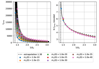
Figure 5: Algorithmic threshold extrapolated using Nesterov acceleration. The dots are the divergence time obtained for the different values of $\Delta_{2}$ with $\Delta_{3}=4.0$ fixed. On the right panel we show that these lines collapse to a single line once rescaled by a factor $a^{\ln m_{x}[0]}$ with $a\approx 1.089$.

The extrapolation procedure for $\Delta_{3}=4.0$ is shown in Fig. 5. The threshold obtained by fitting with a power law and observing the divergent $\Delta_{2}$. On the left panel we plot the number of iteration before the algorithm jumps to the solution $t_{jump}$ as a function of the signal to noise ratio $1/\Delta_{2}$. The figure also show remarkable effects of the initial conditions for $m_{x}$ and $m_{y}$. These effects where already described and understood in Sarao Mannelli et al. (2019b).

Appendix C Correspondence with continuous HB equations

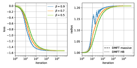
Figure 6: Comparison of HB and massive with mapping. The figure reproduce the same setting of Fig. 2 with the additional dashed line for the DMFT of massive gradient flow using the mapping.

An alternative way to analyze the HB dynamics is by using the results of Qian (1999) to map it to the massive momentum described by the flow equation

$$m\ddot{x}_{i}(t)+\dot{x}_{i}(t)=-\frac{\delta\mathcal{L}[\boldsymbol{x}(t)]}{\delta x_{i}(t)}.$$ (43)

The natural discretization of this equation is

$$\begin{split}&\frac{m}{h^{2}}\left(x[k+1]\!-\!2x[k]\!-\!x[k-1]\right)\!+\!\frac{1}{h}\left(x[k+1]-x[k]\right)=-\nabla\mathcal{L}(x[k])\end{split}$$ (44)

being $h$ the time discretization step (analogous to the learning rate in gradient descent). Using the mapping of Qian (1999) we can identify

$$m =\frac{\beta\alpha}{(1-\beta)^{2}}$$ (45)

$$h =\frac{\alpha}{1-\beta}$$ (46)

Observe that in order to be consistent with a continuous dynamics we need the following scaling $\beta=\mathcal{O}(1)$, $\alpha=\mathcal{O}[(1-\beta)^{2}]$. We empirically observe in the simulations a good agreement between massive and HB even for $\beta=0.999$ and $\alpha=0.01$. In the following, when discussing the comparison between simulation and DMFT, we mean that we run HB algorithm and superimpose on its massive momentum description.

The massive momentum dynamics was also considered in Cugliandolo et al. (2017) without the damping term ($\dot{x}_{i}(t)$) and for the model with a hard spherical constraint $\sum_{i}x_{i}[t]^{2}=N$. While the DMFT derived in Cugliandolo et al. (2017) completely describe the aforementioned particular case, the way in which it is written uses the fact that without damping the dynamics is conservative and the spherical constraint can be enforced using that. In our case we are not in this regime and therefore we resort to a different computation, that will lead us to quite different equations. Indeed if one wants to transform massive momentum in a practical algorithm one needs to transform the second order ODEs into first order by defining velocity variables $v_{i}(t)=\dot{x}_{i}(t)$. Then the discrete version of Eq. equation 43 is

$$\begin{split}x_{i}[t+1]&=x_{i}[t]+hv_{i}[t]\\ v_{i}[t+1]&=v_{i}[t]-\frac{h}{m}\ v_{i}[t]-\frac{h}{m}\ \frac{\delta\mathcal{H}}{\delta x_{i}[t]}\end{split}$$ (47)

Analysing these equations through DMFT one gets a set of flow equations for the following dynamical order parameters $C_{x}[t,t^{\prime}]=\sum_{i}x_{i}[t]x_{i}[t^{\prime}]/N$, $C_{v}[t,t^{\prime}]=\sum_{i}v_{i}[t]v_{i}[t^{\prime}]/N$, $C_{xv}[t,t^{\prime}]=\sum_{i}x_{i}[t]v_{i}[t]/N$, $R_{v}[t,t^{\prime}]=\frac{1}{N}\sum_{i}\frac{\delta v_{i}[t]}{\delta H_{i}[t^{\prime}]}$, and $R_{x|v}[t,t^{\prime}]=\frac{1}{N}\sum_{i}\frac{\delta x_{i}[t]}{\delta H_{i}[t^{\prime}]}$; where $\boldsymbol{H}$ is an instantaneous perturbation acting on the velocity. The result of the computation gives:

$$C_{x}[t+1,t^{\prime}]=C_{x}[t,t^{\prime}]+h\ C_{xv}(t^{\prime},t)\ ;$$ (48)

$$\begin{split}&C_{v}[t+1,t^{\prime}]=C_{v}[t,t^{\prime}]-\frac{h}{m}\ C_{v}(t,t^{\prime})-\mu\ \frac{h}{m}\ C_{xv}(t,t^{\prime})\left(C_{x}(t,t)-1\right)\\ &\quad+\frac{h^{2}}{m}\ \sum_{t^{\prime\prime}=0}^{t}R_{x|v}[t,t^{\prime\prime}]Q^{\prime\prime}\left(C_{x}[t,t^{\prime\prime}]\right)C_{xv}[t^{\prime\prime},t^{\prime}]+\frac{h^{2}}{m}\ \sum_{t^{\prime\prime}=0}^{t^{\prime}}Q^{\prime}\left(C_{x}[t,t^{\prime\prime}]\right)R_{v}[t^{\prime},t^{\prime\prime}];\end{split}$$ (49)

$$C_{xv}[t+1,t^{\prime}]=C_{xv}[t,t^{\prime}]+h\ C_{v}[t,t^{\prime}]\ ;$$ (50)

$$\begin{split}&C_{xv}[t,t^{\prime}+1]=C_{xv}[t,t^{\prime}]-\frac{h}{m}\ C_{xv}[t,t^{\prime}]-\mu\ \frac{h}{m}\ C_{x}[t,t^{\prime}]\left(C_{x}[t^{\prime},t^{\prime}]-1\right)\\ &\quad+\frac{h^{2}}{m}\ \sum_{t^{\prime\prime}=0}^{t^{\prime}}R_{x|v}[t^{\prime},t^{\prime\prime}]Q^{\prime\prime}\left(C_{x}[t^{\prime},t^{\prime\prime}]\right)C_{x}[t,t^{\prime\prime}]+\frac{h^{2}}{m}\ \sum_{t^{\prime\prime}=0}^{t}Q^{\prime}\left(C_{x}[t^{\prime},t^{\prime\prime}]\right)R_{x|v}[t,t^{\prime\prime}]\end{split}$$ (51)

$$\begin{split}&R_{v}[t+1,t^{\prime}]=R_{v}[t,t^{\prime}]+\frac{h}{m}\ \delta_{t,t^{\prime}}-\mu\ \frac{h}{m}\ R_{x|v}[t,t^{\prime}]\left(C_{x}(t,t)-1\right)-\frac{h}{m}\ R_{v}[t,t^{\prime}]\\ &\quad+\frac{h^{2}}{m}\ \sum_{t^{\prime\prime}=0}^{t}Q^{\prime\prime}\left(C[t,t^{\prime\prime}]\right)R_{x|v}[t,t^{\prime\prime}]R_{x|v}[t^{\prime\prime},t^{\prime}]\end{split}$$ (52)

$$R_{x|v}[t+1,t^{\prime}]=R_{x|v}[t,t^{\prime}]+h\ R_{v}[t,t^{\prime}].$$ (53)

and initial conditions : $C_{x}[0,0]=1$, $C_{v}[0,0]=0$, $C_{xv}[0,0]=0$, $R_{v}[t+1,t]=1/m$, $R_{x|v}[t+1,t]=0$.

Derivation of the DMFT equations for massive gradient flow

Figure 7: Comparison of HB and with DMFT. Simulations of HB momentum in the mixed $p$-spin model with $p=3$, $\Delta_{3}=2/p$, $\Delta_{2}=1$, ridge parameter $\mu=10$ and input dimension $N=1024$. The parameters are $\alpha=0.01$ for all the simulations and $\beta\in\{0.5,0.7,0.9,0.99,0.999\}$. We use solid line to represent the result from the simulation, the dotted line for the DMFT of massive gradient flow with the mapping. We empirically observe that in this problem the value of $\beta$ that gives the best speed up is $\beta=0.9$. In order the integrate the DMFT of massive gradient we matched the mass as described in Eq. equation 45 and consider time steps $h\in\{0.005,0.005,0.0125,0.25,0.25\}$.

In this section we derive the dynamical mean field theory (DMFT) equations of massive gradient flow in the mixed $p$-spin.

We use the generating functional approach described in Castellani and Cavagna (2005); Agoritsas et al. (2018) to obtain the effective dynamical equations. First we rewrite de massive dynamics Eq. equation 43 as two ODEs

$$m\dot{\boldsymbol{v}}(t)=-\boldsymbol{v}(t)-\nabla\mathcal{H}[\boldsymbol{x}(t)],$$ (54)

$$\dot{\boldsymbol{x}}(t)=\boldsymbol{v}(t).$$ (55)

We use the following simple identity that takes the name of generating functional

$$1 =\mathcal{Z}=\int\mathcal{D}[\boldsymbol{x},\boldsymbol{v}]\ \delta\left(m\dot{\boldsymbol{v}}(t)+\boldsymbol{v}(t)+\nabla\mathcal{H}[\boldsymbol{x}(t)]\right)\ \delta\left(\dot{\boldsymbol{x}}(t)-\boldsymbol{v}(t)\right)$$ (56)

$$=\int\mathcal{D}[\boldsymbol{x},\tilde{\boldsymbol{x}},\boldsymbol{v},\tilde{\boldsymbol{v}}]\prod_{i=1}^{N}\exp\left\{i\int\tilde{v}_{i}(t)\left[m\dot{v}_{i}(t)+v_{i}(t)+\nabla_{i}\mathcal{H}[\boldsymbol{x}(t)]\right]dt\right\}\exp\left\{i\int\tilde{x}_{i}(t)\left[\dot{x}_{i}(t)-v_{i}(t)\right]dt\right\}$$ (57)

where in the first line we integrate over all possible trajectories of $\boldsymbol{v}$ and $\boldsymbol{x}$, and we impose them to match the massive gradient flow equations using Dirac’s deltas. In the second line we use the Fourier representation of the delta and we absorb the normalization constants in the term $\mathcal{D}[\boldsymbol{x},\tilde{\boldsymbol{x}},\boldsymbol{v},\tilde{\boldsymbol{v}}]$. We can now average over the stochasticity of the problem, let us indicate with an overline the average.

$$1=\overline{\mathcal{Z}} =\int\mathcal{D}[\boldsymbol{x},\tilde{\boldsymbol{x}},\boldsymbol{v},\tilde{\boldsymbol{v}}]\prod_{i=1}^{N}\exp\left\{i\int\tilde{v}_{i}(t)\left[m\dot{v}_{i}(t)+v_{i}(t)\right]dt\right\}\exp\left\{i\int\tilde{x}_{i}(t)\left[\dot{x}_{i}(t)-v_{i}(t)\right]dt\right\}\times$$ (58)

$$\times\overline{\prod_{i=1}^{N}\exp\left\{i\int\tilde{v}_{i}(t)\left[\sqrt{\frac{(p-1)!}{N^{p-1}}}\sum_{(i,i_{2},\dots,i_{p})}\xi_{i,i_{2},\dots,i_{p}}^{(p)}x_{i_{2}}(t)\dots x_{i_{p}}(t)+\frac{1}{\sqrt{N}}\sum_{j}\xi_{i,j}^{(2)}x_{j}(t)\right]dt\right\}}\times$$ (59)

$$\times\prod_{i=1}^{N}\exp\left\{i\int\tilde{v}_{i}(t)\mu\left(\frac{1}{N}\sum_{j}x_{j}^{2}(t)-1\right)x_{i}(t)dt\right\}$$ (60)

We can proceed integrating the second line over the noise. Importantly we must group all the element that multiply a given $\xi^{(p)}$. Considering only second line and neglecting constant multiplicative factors we obtain

$$\exp\Bigg{\{}-\frac{N}{2p\Delta_{p}}\int\Bigg{[}p\left(\sum_{i}\frac{\tilde{v}_{i}(t)\tilde{v}_{i}(t^{\prime})}{N}\right)\left(\sum_{i}\frac{x_{i}(t)x_{i}(t^{\prime})}{N}\right)^{p-1}+$$

$$\quad\quad\quad+p(p-1)\left(\sum_{i}\frac{\tilde{v}_{i}(t)x_{i}(t^{\prime})}{N}\right)\left(\sum_{i}\frac{x_{i}(t)\tilde{v}_{i}(t^{\prime})}{N}\right)\left(\sum_{i}\frac{x_{i}(t)x_{i}(t^{\prime})}{N}\right)^{p-2}\Bigg{]}dt^{\prime}dt\Bigg{\}}\times$$

$$\times\exp\Bigg{\{}-\frac{N}{2\Delta_{2}}\int\Bigg{[}\left(\sum_{i}\frac{\tilde{v}_{i}(t)\tilde{v}_{i}(t^{\prime})}{N}\right)\left(\sum_{i}\frac{x_{i}(t)x_{i}(t^{\prime})}{N}\right)+\left(\sum_{i}\frac{\tilde{v}_{i}(t)x_{i}(t^{\prime})}{N}\right)\left(\sum_{i}\frac{x_{i}(t)\tilde{v}_{i}(t^{\prime})}{N}\right)\Bigg{]}dt^{\prime}dt\Bigg{\}}$$

We define $Q(x)=x^{p}/(p\Delta_{p})+x^{2}/(2\Delta_{2})$ and the order parameters

$$C_{x}[t,t^{\prime}] =\sum_{i}x_{i}[t]x_{i}[t^{\prime}]/N,$$ (61)

$$C_{v}[t,t^{\prime}] =\sum_{i}v_{i}[t]v_{i}[t^{\prime}]/N,$$ (62)

$$C_{xv}[t,t^{\prime}] =\sum_{i}x_{i}[t]v_{i}[t]/N,$$ (63)

$$R_{v}[t,t^{\prime}] =\frac{1}{N}\sum_{i}\frac{\delta v_{i}[t]}{\delta H_{i}[t^{\prime}]},$$ (64)

$$R_{x|v}[t,t^{\prime}] =\frac{1}{N}\sum_{i}\frac{\delta x_{i}[t]}{\delta H_{i}[t^{\prime}]};$$ (65)

and enforce some of them using Dirac’s deltas

$$\int\mathcal{D}[C_{x},C_{\tilde{v}},C_{x\tilde{v}},C_{\tilde{v}x}]\delta\left(NC_{\tilde{v}}(t,t^{\prime})-\sum_{j}\ i\ \tilde{v}_{j}(t)\ i\ \tilde{v}_{j}(t^{\prime})\right)\delta\left(NC_{x}(t,t^{\prime})-\sum_{j}\ x_{j}(t)\ x_{j}(t^{\prime})\right)\times$$

$$\quad\times\delta\left(NC_{x\tilde{v}}(t,t^{\prime})-\sum_{j}\ x_{j}(t)\ i\ \tilde{v}_{j}(t^{\prime})\right)\delta\left(NC_{\tilde{v}x}(t,t^{\prime})-\sum_{j}\ i\ \tilde{v}_{j}(t)\ x_{j}(t^{\prime})\right)\times$$

$$\quad\times\exp\Bigg{\{}-\frac{N}{2\Delta_{p}}\int\Bigg{[}C_{\tilde{v}}(t,t^{\prime})Q^{\prime}\left[C_{x}(t,t^{\prime})\right]+C_{\tilde{v}x}(t,t^{\prime})C_{x\tilde{v}}(t,t^{\prime})Q^{\prime\prime}\left[C_{x}(t,t^{\prime})\right]\Bigg{]}dt^{\prime}dt\Bigg{\}}.$$

Using again the Fourier representation of the deltas and considering $N$ large, the auxiliary variables introduced with the transform concentrate to their saddle point according to Laplace approximation. Furthermore it is easy to show Castellani and Cavagna (2005) that $C_{x\tilde{v}}(t,t^{\prime})=C_{\tilde{v}x}(t^{\prime},t)$ and $C_{x\tilde{v}}(t,t^{\prime})=R_{x|v}(t,t^{\prime})$, with $R_{x|v}$. Under this considerations, we rewrite the average generating functional

$$1=\overline{\mathcal{Z}} =\int\mathcal{D}[\boldsymbol{x},\tilde{\boldsymbol{x}},\boldsymbol{v},\tilde{\boldsymbol{v}}]\prod_{i=1}^{N}\exp\left\{i\int\tilde{v}_{i}(t)\left[m\dot{v}_{i}(t)+v_{i}(t)+\mu\left(\frac{\sum_{j}x_{j}^{2}(t)}{N}-1\right)x_{i}(t)\right]dt\right\}\times$$ (66)

$$\times\prod_{i=1}^{N}\exp\left\{i\int\tilde{x}_{i}(t)\left[\dot{x}_{i}(t)-v_{i}(t)\right]dt\right\}\times$$ (67)

$$\times\exp\left\{-\int\sum_{j}\left[\frac{1}{2}Q^{\prime}[C_{x}(t,t^{\prime})]i\ \tilde{v}_{j}(t)\ i\ \tilde{v}_{j}(t^{\prime})-Q^{\prime\prime}[C_{x}(t,t^{\prime})]R_{x|v}(t,t^{\prime})\ i\ \tilde{v}_{j}(t^{\prime})\ x_{j}(t)\right]dt^{\prime}dt\right\}.$$ (68)

Finally we can take a Hubbard-Stratonovich transform on the first term of the second line and identify a stochastic process $\Xi(t)$ with zero mean at all times and covariance $\mathbb{E}[\Xi(t)\Xi(t^{\prime})]=Q^{\prime}[C_{x}(t,t^{\prime})]$. The resulting generating functional now represent the dynamics in $\boldsymbol{x}$ and $\boldsymbol{v}$ where the cross-element interactions are replaced by the stochastic process. The resulting effective equations are

$$m\dot{\boldsymbol{v}}(t)=-\boldsymbol{v}(t)+\int_{0}^{t}dt^{\prime\prime}R_{x|v}(t,t^{\prime\prime})Q^{\prime}[C_{x}(t,t^{\prime\prime})]\boldsymbol{x}(t^{\prime\prime})+\boldsymbol{\Xi}(t)-\mu\left[C_{x}(t,t)-1\right]\boldsymbol{x}(t),$$ (69)

$$\dot{\boldsymbol{x}}(t)=\boldsymbol{v}(t).$$ (70)

Finally we introduce the order parameters Eqs. (61-65) and compute their equation explicitly by substituting the equations of the effective dynamics. In order to do that, we use Girsanov theorem and evaluate the following expected values

$$\langle v(t)\Xi(t^{\prime})\rangle=\int_{0}^{t^{\prime}}dt^{\prime\prime}R_{v}(t,t^{\prime\prime})Q^{\prime}[C_{x}(t,t^{\prime\prime})],$$ (71)

$$\langle x(t)\Xi(t^{\prime})\rangle=\int_{0}^{t^{\prime}}dt^{\prime\prime}R_{x|v}(t,t^{\prime\prime})Q^{\prime}[C_{x}(t,t^{\prime\prime})].$$ (72)

The dynamical equations are

$$\partial_{t}C_{x}(t,t^{\prime})=C_{xv}(t^{\prime},t)\ ;$$ (73)

$$\begin{split}&m\partial_{t}C_{v}(t,t^{\prime})=-C_{v}(t,t^{\prime})+\int_{0}^{t}dt^{\prime\prime}R_{x|v}(t,t^{\prime\prime})Q^{\prime\prime}[C_{x}(t,t^{\prime\prime})]C_{xv}(t^{\prime\prime},t^{\prime})+\\ &\quad\quad+\int_{0}^{t^{\prime}}Q^{\prime}[C_{x}(t,t^{\prime\prime})]R_{v}(t^{\prime},t^{\prime\prime})-\mu C_{x}(t,t^{\prime})\left(C_{x}(t,t^{\prime})-1\right);\end{split}$$ (74)

$$\partial_{t}C_{xv}(t,t^{\prime})=C_{v}(t,t^{\prime})\ ;$$ (75)

$$\begin{split}&m\partial_{t^{\prime}}C_{xv}(t,t^{\prime})=-C_{xv}(t,t^{\prime})+\int_{0}^{t^{\prime}}dt^{\prime\prime}R_{x|v}(t^{\prime},t^{\prime\prime})Q^{\prime\prime}[C_{x}(t^{\prime},t^{\prime\prime})]C_{x}(t,t^{\prime\prime})+\\ &\quad\quad+\int_{0}^{t}Q^{\prime}[C_{x}(t^{\prime},t^{\prime\prime})]R_{x|v}(t,t^{\prime\prime})-\mu C_{xv}(t,t^{\prime})\left(C_{x}(t,t^{\prime})-1\right);\end{split}$$ (76)

$$\begin{split}&m\partial_{t}R_{v}(t,t^{\prime})=\delta(t-t^{\prime})-R_{v}(t,t^{\prime})+\int_{t^{\prime}}^{t}dt^{\prime\prime}Q^{\prime\prime}[C(t,t^{\prime\prime})]R_{x|v}(t,t^{\prime\prime})R_{x|v}(t^{\prime\prime},t^{\prime})+\\ &\quad\quad-\mu R_{x|v}(t,t^{\prime})\left(C_{x}(t,t^{\prime})-1\right);\end{split}$$ (77)

$$\partial_{t}R_{x|v}(t,t^{\prime})=R_{v}(t,t^{\prime}).$$ (78)

and $\mu(t)=C_{xv}(t,t)$.

The initial conditions are :

$$C_{x}(t,t)=1\ ;$$ (79)

$$C_{v}(t=0,t=0)=0\ ;$$ (80)

$$C_{xv}(t=0,t=0)=0\ ;$$ (81)

$$R_{v}(t^{+},t^{+})=1/m\ ;$$ (82)

$$R_{x|v}(t,t)=0\ .$$ (83)

Where Eq. equation 79 comes from the spherical constraint; Eqs. (80,81) come from the initialization with no kinetic energy $\boldsymbol{v}(0)=\boldsymbol{0}$; Eqs. equation 82 and equation 83 come from Eqs. equation 69 and equation 70 (respectively) after deriving by $\Xi(t^{\prime})$, integrating on $t$ in $[t-h;t+h]$ (with $h\rightarrow 0$) and taking $t^{\prime}\rightarrow t$. The equations shown in the main text are the discrete equivalent of the ones just obtained.

Appendix D Hard spherical constraint

It is also possible to consider a hard spherical constraint, which is the situation typically considered in the physics literature Crisanti and Sommers (1992); Cugliandolo and Kurchan (1993). A massive dynamics was already considered in Cugliandolo et al. (2017) but their derivation was in the underdamped regime where the total energy is conserved. Using that approach the conservation of the energy was key. Unfortunately the energy is not conserved in general, and in particular in the case of optimization where we aim to go down in energy in order to find a minimum.

For reference sake we consider massive gradient flow, the same considerations apply straightforwardly to Nesterov acceleration. Let us write the dynamics in this case splitting the system in two ODEs

$$m\dot{\boldsymbol{v}}(t)=-\boldsymbol{v}(t)-\nabla\mathcal{L}[\boldsymbol{x}(t)],$$ (84)

$$\dot{\boldsymbol{x}}(t)=\boldsymbol{v}(t)-\mu(t)\boldsymbol{x}(t).$$ (85)

The last term in the second line constraints the dynamics to move in the sphere by removing the terms of the velocity that move orthogonally to the sphere. Therefore the term $\mu(t)$ is given by the projection of the velocity in the direction that is tangent to the sphere $\sum_{j}x_{j}(t)v_{j}(t)/N$.

We can then follow the usual techniques, e.g. section C, and obtain

$$\partial_{t}C_{x}(t,t^{\prime})=-\mu(t)C_{x}(t,t^{\prime})+C_{xv}(t^{\prime},t)\ ,$$ (86)

$$m\partial_{t}C_{v}(t,t^{\prime})=-C_{v}(t,t^{\prime})+\int_{0}^{t}dt^{\prime\prime}R_{x|v}(t,t^{\prime\prime})Q^{\prime\prime}[C_{x}(t,t^{\prime\prime})]C_{xv}(t^{\prime\prime},t^{\prime})+\int_{0}^{t^{\prime}}Q^{\prime}[C_{x}(t,t^{\prime\prime})]R_{v}(t^{\prime},t^{\prime\prime})\ ,$$ (87)

$$\partial_{t}C_{xv}(t,t^{\prime})=-\mu(t)C_{xv}(t,t^{\prime})+C_{v}(t,t^{\prime})\ ,$$ (88)

$$m\partial_{t^{\prime}}C_{xv}(t,t^{\prime})=-C_{xv}(t,t^{\prime})+\int_{0}^{t^{\prime}}dt^{\prime\prime}R_{x|v}(t^{\prime},t^{\prime\prime})Q^{\prime\prime}[C_{x}(t^{\prime},t^{\prime\prime})]C_{x}(t,t^{\prime\prime})+\int_{0}^{t}Q^{\prime}[C_{x}(t^{\prime},t^{\prime\prime})]R_{x|v}(t,t^{\prime\prime})\ ,$$ (89)

$$m\partial_{t}R_{v}(t,t^{\prime})=\delta(t-t^{\prime})-R_{v}(t,t^{\prime})+\int_{t^{\prime}}^{t}dt^{\prime\prime}Q^{\prime\prime}[C(t,t^{\prime\prime})]R_{x|v}(t,t^{\prime\prime})R_{x|v}(t^{\prime\prime},t^{\prime})\ ,$$ (90)

$$\partial_{t}R_{x|v}(t,t^{\prime})=-\mu(t)R_{x|v}(t,t^{\prime})+R_{v}(t,t^{\prime});$$ (91)

with $\mu(t)=C_{xv}(t,t)$ and initial conditions $C_{x}(t,t)=1$, $C_{v}(0,0)=0$, $C_{xv}(0,0)=0$, $R_{v}(t^{+},t)=\frac{1}{m}$, $R_{x|v}(t,t)=0$.

References

• Agoritsas et al. (2018) Elisabeth Agoritsas, Giulio Biroli, Pierfrancesco Urbani, and Francesco Zamponi. Out-of-equilibrium dynamical mean-field equations for the perceptron model. Journal of Physics A: Mathematical and Theoretical, 51(8):085002, 2018.
• An et al. (2018) Wangpeng An, Haoqian Wang, Qingyun Sun, Jun Xu, Qionghai Dai, and Lei Zhang. A pid controller approach for stochastic optimization of deep networks. In Proceedings of the IEEE Conference on Computer Vision and Pattern Recognition, pages 8522–8531, 2018.
• Auffinger et al. (2013) Antonio Auffinger, Gérard Ben Arous, and Jiří Černỳ. Random matrices and complexity of spin glasses. Communications on Pure and Applied Mathematics, 66(2):165–201, 2013.
• Barrat et al. (1997) Alain Barrat, Silvio Franz, and Giorgio Parisi. Temperature evolution and bifurcations of metastable states in mean-field spin glasses, with connections with structural glasses. Journal of Physics A: Mathematical and General, 30(16):5593–5612, aug 1997. doi: 10.1088/0305-4470/30/16/006. URL https://doi.org/10.1088/0305-4470/30/16/006.
• Ben Arous et al. (2006) Gérard Ben Arous, Amir Dembo, and Alice Guionnet. Cugliandolo-Kurchan equations for dynamics of spin-glasses. Probability theory and related fields, 136(4):619–660, 2006.
• Broyden (1970) Charles G Broyden. The convergence of a class of double-rank minimization algorithms: 2. the new algorithm. IMA journal of applied mathematics, 6(3):222–231, 1970.
• Can et al. (2020) Tankut Can, Kamesh Krishnamurthy, and David J Schwab. Gating creates slow modes and controls phase-space complexity in grus and lstms. In Mathematical and Scientific Machine Learning, pages 476–511. PMLR, 2020.
• Castellani and Cavagna (2005) Tommaso Castellani and Andrea Cavagna. Spin-glass theory for pedestrians. Journal of Statistical Mechanics: Theory and Experiment, 2005(05):P05012, 2005.
• Cauchy (1847) Augustin Cauchy. Méthode générale pour la résolution des systemes d’équations simultanées. Comp. Rend. Sci. Paris, 25(1847):536–538, 1847.
• Crisanti and Leuzzi (2006) Andrea Crisanti and Luca Leuzzi. Spherical 2+ p spin-glass model: An analytically solvable model with a glass-to-glass transition. Physical Review B, 73(1):014412, 2006.
• Crisanti and Sommers (1992) Andrea Crisanti and H-J Sommers. The sphericalp-spin interaction spin glass model: the statics. Zeitschrift für Physik B Condensed Matter, 87(3):341–354, 1992.
• Crisanti et al. (1993) Andrea Crisanti, Heinz Horner, and H-J Sommers. The sphericalp-spin interaction spin-glass model. Zeitschrift für Physik B Condensed Matter, 92(2):257–271, 1993.
• Cugliandolo and Kurchan (1993) Leticia F Cugliandolo and Jorge Kurchan. Analytical solution of the off-equilibrium dynamics of a long-range spin-glass model. Physical Review Letters, 71(1):173, 1993.
• Cugliandolo et al. (2017) Leticia F Cugliandolo, Gustavo S Lozano, and Emilio N Nessi. Non equilibrium dynamics of isolated disordered systems: the classical hamiltonian p-spin model. Journal of Statistical Mechanics: Theory and Experiment, 2017(8):083301, 2017.
• Cyrus et al. (2018) Saman Cyrus, Bin Hu, Bryan Van Scoy, and Laurent Lessard. A robust accelerated optimization algorithm for strongly convex functions. In 2018 Annual American Control Conference (ACC), pages 1376–1381. IEEE, 2018.
• De Dominicis (1978) C De Dominicis. Dynamics as a substitute for replicas in systems with quenched random impurities. Physical Review B, 18(9):4913, 1978.
• Dembo and Subag (2020) Amir Dembo and Eliran Subag. Dynamics for spherical spin glasses: disorder dependent initial conditions. Journal of Statistical Physics, pages 1–50, 2020.
• Flammarion and Bach (2015) Nicolas Flammarion and Francis Bach. From averaging to acceleration, there is only a step-size. In Conference on Learning Theory, pages 658–695. PMLR, 2015.
• Fletcher (1970) Roger Fletcher. A new approach to variable metric algorithms. The computer journal, 13(3):317–322, 1970.
• Folena et al. (2020) Giampaolo Folena, Silvio Franz, and Federico Ricci-Tersenghi. Rethinking mean-field glassy dynamics and its relation with the energy landscape: The surprising case of the spherical mixed p-spin model. Physical Review X, 10(3):031045, 2020.
• Folena et al. (2021) Giampaolo Folena, Silvio Franz, and Federico Ricci-Tersenghi. Gradient descent dynamics in the mixed p-spin spherical model: finite-size simulations and comparison with mean-field integration. Journal of Statistical Mechanics: Theory and Experiment, 2021(3):033302, 2021.
• Gadat et al. (2018) Sébastien Gadat, Fabien Panloup, Sofiane Saadane, et al. Stochastic heavy ball. Electronic Journal of Statistics, 12(1):461–529, 2018.
• Ghadimi et al. (2015) Euhanna Ghadimi, Hamid Reza Feyzmahdavian, and Mikael Johansson. Global convergence of the heavy-ball method for convex optimization. In 2015 European control conference (ECC), pages 310–315. IEEE, 2015.
• Gitman et al. (2019) Igor Gitman, Hunter Lang, Pengchuan Zhang, and Lin Xiao. Understanding the role of momentum in stochastic gradient methods. In H. Wallach, H. Larochelle, A. Beygelzimer, F. d Alché-Buc, E. Fox, and R. Garnett, editors, Advances in Neural Information Processing Systems, volume 32, pages 9633–9643. Curran Associates, Inc., 2019. URL https://proceedings.neurips.cc/paper/2019/file/4eff0720836a198b6174eecf02cbfdbf-Paper.pdf.
• Goldfarb (1970) Donald Goldfarb. A family of variable-metric methods derived by variational means. Mathematics of computation, 24(109):23–26, 1970.
• Kidambi et al. (2018) Rahul Kidambi, Praneeth Netrapalli, Prateek Jain, and Sham Kakade. On the insufficiency of existing momentum schemes for stochastic optimization. In 2018 Information Theory and Applications Workshop (ITA), pages 1–9. IEEE, 2018.
• Krzakala and Zdeborová (2013) Florent Krzakala and Lenka Zdeborová. Performance of simulated annealing in p-spin glasses. In Journal of Physics: Conference Series, volume 473, page 012022. IOP Publishing, 2013.
• Lessard et al. (2016) Laurent Lessard, Benjamin Recht, and Andrew Packard. Analysis and design of optimization algorithms via integral quadratic constraints. SIAM Journal on Optimization, 26(1):57–95, 2016.
• Levenberg (1944) Kenneth Levenberg. A method for the solution of certain non-linear problems in least squares. Quarterly of applied mathematics, 2(2):164–168, 1944.
• Loizou and Richtárik (2020) Nicolas Loizou and Peter Richtárik. Momentum and stochastic momentum for stochastic gradient, newton, proximal point and subspace descent methods. Computational Optimization and Applications, 77(3):653–710, 2020.
• Ma and Yarats (2019) Jerry Ma and Denis Yarats. Quasi-hyperbolic momentum and adam for deep learning. In 7th International Conference on Learning Representations, ICLR 2019, New Orleans, LA, USA, May 6-9, 2019. OpenReview.net, 2019. URL https://openreview.net/forum?id=S1fUpoR5FQ.
• Marquardt (1963) Donald W Marquardt. An algorithm for least-squares estimation of nonlinear parameters. Journal of the society for Industrial and Applied Mathematics, 11(2):431–441, 1963.
• Martin et al. (1973) Paul Cecil Martin, ED Siggia, and HA Rose. Statistical dynamics of classical systems. Physical Review A, 8(1):423, 1973.
• Mastrogiuseppe and Ostojic (2017) Francesca Mastrogiuseppe and Srdjan Ostojic. Intrinsically-generated fluctuating activity in excitatory-inhibitory networks. PLoS computational biology, 13(4):e1005498, 2017.
• Mézard et al. (1987) Marc Mézard, Giorgio Parisi, and Miguel Angel Virasoro. Spin glass theory and beyond: An Introduction to the Replica Method and Its Applications, volume 9. World Scientific Publishing Company, 1987.
• Mignacco et al. (2020) Francesca Mignacco, Florent Krzakala, Pierfrancesco Urbani, and Lenka Zdeborová. Dynamical mean-field theory for stochastic gradient descent in gaussian mixture classification. In 2020 Conference on Neural Information Processing Systems-NeurIPS 2020, 2020.
• Mignacco et al. (2021) Francesca Mignacco, Pierfrancesco Urbani, and Lenka Zdeborová. Stochasticity helps to navigate rough landscapes: comparing gradient-descent-based algorithms in the phase retrieval problem. Machine Learning: Science and Technology, 2021.
• Nesterov (1983) Yurii E Nesterov. A method for solving the convex programming problem with convergence rate o (1/k^ 2). In Dokl. akad. nauk Sssr, volume 269, pages 543–547, 1983.
• Polyak (1964) Boris T Polyak. Some methods of speeding up the convergence of iteration methods. USSR Computational Mathematics and Mathematical Physics, 4(5):1–17, 1964.
• Qian (1999) Ning Qian. On the momentum term in gradient descent learning algorithms. Neural networks, 12(1):145–151, 1999.
• Richard and Montanari (2014) Emile Richard and Andrea Montanari. A statistical model for tensor pca. In Z. Ghahramani, M. Welling, C. Cortes, N. Lawrence, and K. Q. Weinberger, editors, Advances in Neural Information Processing Systems, volume 27, pages 2897–2905. Curran Associates, Inc., 2014. URL https://proceedings.neurips.cc/paper/2014/file/b5488aeff42889188d03c9895255cecc-Paper.pdf.
• Robbins and Monro (1951) Herbert Robbins and Sutton Monro. A stochastic approximation method. The annals of mathematical statistics, pages 400–407, 1951.
• Sarao Mannelli et al. (2019a) Stefano Sarao Mannelli, Giulio Biroli, Chiara Cammarota, Florent Krzakala, and Lenka Zdeborová. Who is afraid of big bad minima? analysis of gradient-flow in spiked matrix-tensor models. In Advances in Neural Information Processing Systems, pages 8679–8689, 2019a.
• Sarao Mannelli et al. (2019b) Stefano Sarao Mannelli, Florent Krzakala, Pierfrancesco Urbani, and Lenka Zdeborová. Passed & spurious: Descent algorithms and local minima in spiked matrix-tensor models. In International Conference on Machine Learning, pages 4333–4342, 2019b.
• Sarao Mannelli et al. (2020a) Stefano Sarao Mannelli, Giulio Biroli, Chiara Cammarota, Florent Krzakala, Pierfrancesco Urbani, and Lenka Zdeborová. Complex dynamics in simple neural networks: Understanding gradient flow in phase retrieval. In H. Larochelle, M. Ranzato, R. Hadsell, M. F. Balcan, and H. Lin, editors, Advances in Neural Information Processing Systems, volume 33, pages 3265–3274. Curran Associates, Inc., 2020a. URL https://proceedings.neurips.cc/paper/2020/file/2172fde49301047270b2897085e4319d-Paper.pdf.
• Sarao Mannelli et al. (2020b) Stefano Sarao Mannelli, Giulio Biroli, Chiara Cammarota, Florent Krzakala, Pierfrancesco Urbani, and Lenka Zdeborová. Marvels and pitfalls of the langevin algorithm in noisy high-dimensional inference. Physical Review X, 10(1):011057, 2020b.
• Scieur and Pedregosa (2020) Damien Scieur and Fabian Pedregosa. Universal average-case optimality of polyak momentum. In Hal Daumé III and Aarti Singh, editors, Proceedings of the 37th International Conference on Machine Learning, volume 119 of Proceedings of Machine Learning Research, pages 8565–8572. PMLR, 13–18 Jul 2020. URL http://proceedings.mlr.press/v119/scieur20a.html.
• Semerjian et al. (2004) Guilhem Semerjian, Leticia F Cugliandolo, and Andrea Montanari. On the stochastic dynamics of disordered spin models. Journal of statistical physics, 115(1):493–530, 2004.
• Shanno (1970) David F Shanno. Conditioning of quasi-newton methods for function minimization. Mathematics of computation, 24(111):647–656, 1970.
• Sompolinsky et al. (1988) Haim Sompolinsky, Andrea Crisanti, and Hans-Jurgen Sommers. Chaos in random neural networks. Physical review letters, 61(3):259, 1988.
• Su et al. (2014) Weijie Su, Stephen Boyd, and Emmanuel Candes. A differential equation for modeling nesterov’s accelerated gradient method: Theory and insights. Advances in neural information processing systems, 27:2510–2518, 2014.
• Sun et al. (2019) Tao Sun, Penghang Yin, Dongsheng Li, Chun Huang, Lei Guan, and Hao Jiang. Non-ergodic convergence analysis of heavy-ball algorithms. In Proceedings of the AAAI Conference on Artificial Intelligence, volume 33, pages 5033–5040, 2019.
• Sutskever et al. (2013) Ilya Sutskever, James Martens, George Dahl, and Geoffrey Hinton. On the importance of initialization and momentum in deep learning. In International conference on machine learning, pages 1139–1147. PMLR, 2013.
• Wang and Abernethy (2020) Jun-Kun Wang and Jacob Abernethy. Quickly finding a benign region via heavy ball momentum in non-convex optimization. arXiv preprint arXiv:2010.01449, 2020.
• Yang et al. (2016) Tianbao Yang, Qihang Lin, and Zhe Li. Unified convergence analysis of stochastic momentum methods for convex and non-convex optimization. arXiv preprint arXiv:1604.03257, 2016.