Classifying high-dimensional Gaussian mixtures:
Where kernel methods fail and neural networks succeed

Abstract

A recent series of theoretical works showed that the dynamics of neural networks with a certain initialisation are well-captured by kernel methods. Concurrent empirical work demonstrated that kernel methods can come close to the performance of neural networks on some image classification tasks.These results raise the question of whether neural networks only learn successfully if kernels also learn successfully, despite neural nets being more expressive. Here, we show theoretically that two-layer neural networks (2LNN) with only a few neurons can beat the performance of kernel learning on a simple Gaussian mixture classification task. We study the high-dimensional limit, i.e. when the number of samples is linearly proportional to the dimension, and show that while small 2LNN achieve near-optimal performance on this task, lazy training approaches such as random features and kernel methods do not.Our analysis is based on the derivation of a closed set of equations that track the learning dynamics of the 2LNN and thus allow to extract the asymptotic performance of the network as a function of signal-to-noise ratio and other hyperparameters. We finally illustrate how over-parametrising the neural network leads to faster convergence, but does not improve its final performance.

1 Introduction

Explaining the success of deep neural networks in many areas of machine learning remains a key challenge for learning theory. A series of recent theoretical works made progress towards this goal by proving trainability of two-layer neural networks (2LNN) with gradient-based methods (Jacot et al., 2018; Allen-Zhu et al., 2018; Li & Liang, 2018; Allen-Zhu et al., 2019; Cao & Gu, 2019; Du et al., 2019). These results are based on the observation that strongly over-parameterised 2LNN can achieve good performance even if their first-layer weights remain almost constant throughout training. This is the case if the initial weights are chosen with a particular scaling, which was dubbed the “lazy regime” by Chizat et al. (2019). Going a step further, simply fixing the first-layer weights of a 2LNN at their initial values yields the well-known random features model of Rahimi & Recht (2008, 2009), and can be seen as an approximation of kernel learning (Scholkopf & Smola, 2018). This behaviour is to be contrasted with the “feature learning regime”, where the weights of the first layer move significantly during training. Recent empirical studies showed that on some benchmark data sets in computer vision, kernels derived from neural networks achieve comparable performance to neural networks (Matthews et al., 2018; Lee et al., 2018; Garriga-Alonso et al., 2019; Arora et al., 2019; Li et al., 2019; Shankar et al., 2020).

These results raise the question of whether neural networks only learn successfully if random features can also learn successfully, and have led to a renewed interest in the exact conditions under which neural networks trained with gradient descent achieve a better performance than random features (Bach, 2017; Yehudai & Shamir, 2019; Wei et al., 2019; Li et al., 2020; Daniely & Malach, 2020; Geiger et al., 2020; Paccolat et al., 2021; Suzuki & Akiyama, 2020). Chizat & Bach (2020) studied the implicit bias of wide two-layer networks trained on data with a low-dimensional structure. They derived strong generalisation bounds, which, when both layers of the network are trained, are independent of ambient dimensions, indicating that the network is able to adapt to the low dimensional structure. In contrast, when only the output layer of the network is trained, the network does not possess such an adaptivity, leading to worse performance. Ghorbani et al. (2019, 2020) analysed in detail how data structure breaks the curse of dimensionality in wide two-layer neural networks, but not in learning with random features, leading to better performance of the former.

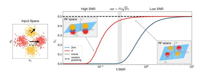
Figure 1: Random Features and 2LNN on high-dimensional Gaussian mixture classification (Left) Consider a data distribution that is a mixture of four Gaussians in $D$ dimensions. The first two components of the centroids organized in a XOR-like manner as shown, while the other $D-2$ directions of the centroids are set to zero. The signal-to-noise is $\operatorname{\sf snr}=\nicefrac{{|\mu|}}{{\sqrt{D}\sigma}}$. We used $\mu=\sqrt{D}$ so the $\operatorname{\sf snr}$ is effectively given by the inverse of the width of the Gaussian: $\operatorname{\sf snr}=1/\sigma$. (Right) A two-layer neural network with $K=4$ hidden neurons and ReLU non-linearity trained using stochastic gradient descent, achieves a long-time test error close to the optimal (oracle) error (3) for the whole range of $\operatorname{\sf snr}$. The test error is obtained analytically using techniques described in Sec. (2.3). In sharp contrast, random features (RF), whose performance is given by Eq. (16), require a high $\operatorname{\sf snr}$ to perform as well as the oracle. They performs better than chance when $\operatorname{\sf snr}\gg\sqrt{D}/\min(P,N)^{1/4}$, and thus requires a diverging $\operatorname{\sf snr}$ in the high-dimensional limit. The insets show the mixture after applying random features; only at high $\operatorname{\sf snr}$ does the mixture become linearly separable. Parameters: RF error is computed with $D=10000$ and $P=2D$ and the 2LNN’s with $D=1000$. For both methods $\eta=0.1$, $\nicefrac{{|\mu|}}{{\sqrt{D}}}=1$.

1.1 Main contributions

We show that even a two-layer neural network with only a few hidden neurons outperforms kernel methods on the classical problem of Gaussian mixture classification. We give a sharp asymptotic analysis of 2LNN and random features on Gaussian mixture classification in the high-dimensional regime where the number of samples $N$ is linearly proportional to the input dimension $D\to\infty$. More precisely:

1. We analyse 2LNN by deriving a closed set of ordinary differential equations (ODEs), which track the test error of 2LNN with a few hidden neurons $K\!\sim\!O(1)$ trained using one-pass (or online) SGD on Gaussian mixture classification. We thereby extend the classical ODE analysis of Riegler & Biehl (1995); Saad & Solla (1995a) where the label $y(x)$ is a function of the input $x$, to a setup where the input is conditional on the label. Solving these equations for their asymptotic fixed point, i.e. taking $t\to\infty$ after $D\to\infty$, yields the final classification error of the 2LNN.

2. Keeping in mind the high-dimensional limit where the number of samples $N$ is proportional to $D$, We analyse how Gaussian mixtures are transformed under $P$ random features in the regime $P,D\to\infty$ with $\gamma\equiv\nicefrac{{P}}{{D}}$ fixed. In the high-dimensional limit the performance at large $\gamma$ converges to the one of the corresponding kernel (Rahimi & Recht, 2008, 2009; El Karoui, 2010; Pennington & Worah, 2017; Louart et al., 2018; Liao & Couillet, 2018), and we can thus recover the performance of kernel learning by taking $\gamma$ large enough.

3. We compute the asymptotic generalisation of random features on mixtures of Gaussians, which allows us to compare their performance to the performance of 2LNN for various signal-to-noise ratios.

While we do not attempt formal rigorous derivations, to keep the paper readable, our theoretical claims are however amenable to rigorous theorems. In particular the ODEs analysis could be formalised rigorously using the technique of (Wang et al., 2019; Goldt et al., 2019). Our results are valid for generic Gaussian Mixtures with $O(1)$ clusters and we focus on the particular example of the XOR-like mixture in order to make the problematic clear.

1.2 A paradigmatic example

Our results can be illustrated with a data distribution where inputs are distributed in a mixture of four Gaussians, whose centres form a XOR-function, and thus cannot be linearly separated in direct space. We find that neural networks with a few neurons have no problems learning a good partitioning of the space in this situation, reaching oracle-like performance in the process. Kernel methods, however, manage to do so only if the centres are extremely well separated, and completely fail when they are too close. This is illustrated in Fig. 1: Inputs $x=(x_{r})\in\mathbb{R}^{D}$ are drawn from the Gaussian mixture shown on the left, where inputs in red, yellow have labels $y=~{}1,-1$, respectively. The first two components of the means are organised as in the diagram, while the remaining $D-2$ components are zero, yielding a XOR-like pattern. Each Gaussian cloud has standard deviation $\sigma\mathbb{I}_{D}$, as Gaussian noise is added to all components of the input, resulting in an $\operatorname{\sf snr}$ of $\nicefrac{{|\mu|}}{{\sqrt{D\sigma^{2}}}}$.

We compare the performance of a two-layer neural network $\phi_{\theta}$ with parameters $\theta=(K,v,W,g)$,

$$\phi_{\theta}(x)=\sum_{k=1}^{K}v^{k}\,g\left(\lambda^{k}\right),\quad\lambda^{k}\equiv\frac{1}{\sqrt{D}}\sum_{r=1}^{D}w^{k}_{r}x_{r},$$ (1)

where $v=(v^{k})\in\mathbb{R}^{K}$ and $W=(w^{k}_{r})\in\mathbb{R}^{K\times D}$ are the weights of the network and $g:\mathbb{R}\to\mathbb{R}$ is a non-linear function shown above only has $K=4$ neurons, and we keep $K$ of order 1 compared to the input dimension $D~{}\to~{}\infty$ throughout this paper. We train the 2LNN using online stochastic gradient descent, where at each step of the algorithm, we draw a new sample from the mixture. We study the high-dimensional limit $t\equiv\nicefrac{{N}}{{D}}=O(1),$ and obtain the final performance of the 2LNN in the limit $t\to\infty$ (after $D\to\infty$) of the ODEs we derive in Sec. 2.2. In blue, we plot the final classification error

$$\epsilon_{c}(\theta)=\mathop{\mathbb{E}\,}\Theta\left[-y\phi_{\theta}(x)\right],$$ (2)

where the expectation $\mathbb{E}\,$ is computed over the Gaussian mixture for a network with fixed parameters $\theta$ and $\Theta$ is the Heaviside step function. The classification error of the 2LNN is very close to that of an oracle with knowledge of the means of the mixture that assigns to each input the label of the nearest mean, achieving a classification error of

$$\epsilon_{c}^{\text{oracle}}=\nicefrac{{1}}{{2}}\left(1-\operatorname{erf}\left(\nicefrac{{|\mu|}}{{2\sigma\sqrt{D}}}\right)^{2}\right).$$ (3)

We compare the performance of the 2LNN to the performance of random features (Rahimi & Recht, 2008, 2009), where we first project the inputs $x$ to a higher-dimensional feature space, where features $z=(z_{i})\in\mathbb{R}^{P}$ are given by

$$z_{i}=\psi(u_{i}),\qquad u_{i}\equiv\sum_{r=1}^{D}\frac{1}{\sqrt{D}}F_{ir}x_{r}\,,$$ (4)

where $F\in\mathbb{R}^{P\times D}$ is a random, but fixed projection matrix and $\psi:\mathbb{R}\to\mathbb{R}$ is an element-wise non-linearity. The features are then fit by training a linear model,

$$\phi_{\theta}(z)=\frac{1}{\sqrt{P}}\sum_{i=1}^{P}w_{i}z_{i},$$ (5)

with weights $w\in\mathbb{R}^{P}$, using SGD, where we again draw a fresh sample from the mixture to evaluate the gradients at each step. The performance of RF is shown in red in Fig. 1. While RF achieve low classification error at high $\operatorname{\sf snr}$, there is a wide range of $\operatorname{\sf snr}$ where random features do significantly worse than the 2LNN. The insets give the intuition behind this result: at high $\operatorname{\sf snr}$, RF map the inputs into linearly separable mixture in random feature space (left) while at lower ${\rm snr}$, the transformed mixture is not linearly separable in RF space (right), leading to poor performance.

We emphasise that we study random features in the high-dimensional limit where we let $N,D\to\infty$ with their ratio $t=\nicefrac{{N}}{{D}}\!\sim\!O(1)$ as before, while also letting the number of random features $P\to\infty$ with their ratio $\gamma\equiv\nicefrac{{P}}{{D}}\sim O(1)$ fixed. This regime has been studied in a series of recent works (Lelarge & Miolane, 2019; Couillet, 2019; Liao & Couillet, 2019; Mai & Liao, 2019; Deng et al., 2019; Kini & Thrampoulidis, 2020; Mignacco et al., 2020a). While we concentrate on random features, we note that we can recover the performance of kernel methods (Rahimi & Recht, 2008, 2009) by sending $\gamma\to\infty$. Indeed, as $\gamma=\nicefrac{{P}}{{D}}$ grows, the gram matrix converges to the limiting kernel gram matrix in the high-dimensional regime; detailed studies of the convergence in this regime can be found in (El Karoui, 2010; Pennington & Worah, 2017; Louart et al., 2018; Liao & Couillet, 2018). We can thus recover the performance for any general distance or angle based kernel method, e.g. the NTK of Jacot et al. (2018), by considering $\gamma$ large enough in our computations with random features. Note, however, that this must be done with some care. Our results for random projections are given for $N>P$. As discussed by Ghorbani et al. (2019); Mei et al. (2021), the relevant dimension for random features performances is, rather than $P$, the minimum between $N$ and $P$. Since we focus here in the regime where increasing $P$ beyond $O(D)$, and therefore $\gamma$ beyond $O(1)$, is not allowed. Indeed, we shall see that Lazy training methods such as kernels or random projections require asymptotically $N=O(D^{2})$ samples to beat a random guess, while neural-networks achieves oracle-like performances with only $N=O(D)$ samples.

Reproducibility

We provide code to reproduce our plots and solve the equations of Sec. 2.2 at  github.com/mariaref/rfvs2lnn_GMM_online.

1.3 Further related work

Separation between kernels & 2LNN

Barron (1993) already discussed the limitations of approximating functions with a bounded number of random features within a worst-case analysis. Yehudai & Shamir (2019) construct a data distribution that can be efficiently learnt by a single ReLU neuron, but not by random features. Wei et al. (2019) studied the separation between 2LNN & RF and show the existence of a small ($K\sim O(1)$) network that beats kernels on this data distribution, and study the dynamics of learning in the same mean-field limit as Chizat & Bach (2020) and Ghorbani et al. (2019, 2020). Likewise, Li et al. (2020) show separation between kernels & neural networks in the mean-field limit on the phase retrieval problem. Geiger et al. (2020) investigated numerically the role of architecture and data in determining whether lazy or feature learning perform better. Paccolat et al. (2021) studied how neural networks can compress inputs of effectively low-dimensional data.

Gaussian mixture classification

is a well-studied problem in statistical learning theory, and its supervised version was recently considered in a series of works from the perspective of Bayes-optimal inference (Lelarge & Miolane, 2019; Mai & Liao, 2019; Deng et al., 2019). Mignacco et al. (2020a, b) studied the dynamics of stochastic gradient descent on a finite training set using dynamical mean-field theory for the perceptron, which corresponds to the case $K=1,v^{1}=1$ in Eq. (1). Liao & Couillet (2019) and Couillet (2019) studied mixture classification with kernel in an unsupervised setting using random matrix theory.

Dynamics of 2LNN

A classic series of papers by Biehl & Schwarze (1995) and Saad & Solla (1995a) studied the dynamics of 2LNN as in Eq. (1) trained using online SGD in the classic teacher-student setup (Gardner & Derrida, 1989), where inputs $x$ are element-wise i.i.d. Gaussian variables and labels are obtained from a “teacher” network with random weights. They derived a set of closed ODEs that track the test error of the student (see also Saad & Solla (1995b); Biehl et al. (1996); Saad (2009) for further results and Goldt et al. (2019) for a recent proof of these equations). There have been several extensions of this approach to different data distributions (Yoshida & Okada, 2019; Goldt et al., 2020b, a). All of these works, though, consider the label $y$ as a function of the input $x$, or as a function of a latent variable from which $x$ is generated. Here, we extend this type of analysis to a case where the input is conditional on the label, a point of view taken implicitly by Cohen et al. (2020).

The reduction of the dynamics to a set of low-dimensional ODEs should be contrasted with the “mean-field” approach, where the number of hidden neurons $K$ is sent to infinity while the input dimension $D$ is kept finite. In this limit, the neural networks are still a more expressive function class than the corresponding reproducing kernel Hilbert space (Chizat & Bach, 2018; Sirignano & Spiliopoulos, 2019; Rotskoff & Vanden-Eijnden, 2018; Mei et al., 2018). The evolution of the network parameters in this limit can be described by a high-dimensional partial differential equation. This analysis was used in the aforementioned works by Ghorbani et al. (2019, 2020).

2 Neural networks for GM classification

2.1 Setup

We draw inputs $x\!=\!(x_{i})\!\in\!\mathbb{R}^{D}$ from a high-dimensional Gaussian mixture, where all samples from one Gaussian are assigned to one of two possible labels $y=\!\pm 1$, which are equiprobable. The data distribution is thus

$$q(x,y)\!=\!q(y)q(x|y),\quad\!\!\!q(x|y)\!=\!\!\!\!\!\sum_{\alpha\in\mathcal{S}\left(y\right)}\!\!\!\!\!\mathcal{P}_{\alpha}\mathcal{N}_{\alpha}(x)\,,$$ (6)

where $\mathcal{N}_{\alpha}(x)$ is a multivariate normal distribution with mean $\nicefrac{{\mu^{\alpha}}}{{\sqrt{D}}}$ and covariance $\Omega^{\alpha}$. The index set $\mathcal{S}(y)$ contains all the Gaussians that are associated with the label $y$. We choose the constants $\mathcal{P}_{\alpha}$ such that $q(x,y)$ is correctly normalised. To simplify notation, we focus on binary classification, which can be learnt using a student with a single output unit. Extending our results to $C$-class classification, where the student has $C$ output heads, is straightforward.

Training

The network is trained using stochastic gradient descent on the quadratic error for technical reasons related to the analysis. The update equations for the weights at the $\mu$th step of the algorithm, $\operatorname{d}\!w^{k}_{i}\equiv\left(w^{k}_{i}\right)_{\mu+1}-\left(w^{k}_{i}\right)_{\mu}$, read

$$\operatorname{d}\!w^{k}_{i} =-\frac{\eta}{\sqrt{D}}v^{k}\Delta g^{\prime}(\lambda^{k})x_{i}-\frac{\eta}{\sqrt{D}}\kappa w^{k}_{i},$$ (7a)

$$\operatorname{d}\!v^{k} =-\frac{\eta}{D}g(\lambda^{k})\Delta-\frac{\eta}{D}\kappa v^{k}\,,$$ (7b)

where $\Delta\!=\!\sum_{j=1}^{K}\!v^{j}g(\lambda^{j})\!-\!y$ and $\kappa\!\in\!\mathbb{R}$ is a $L_{2}$-regularisation constant. Initial weights are taken i.i.d. from the normal distribution with standard deviation $\sigma_{0}$. The different scaling of the learning rates $\eta$ for first and second-layer weights guarantees the existence of a well-defined limit of the SGD dynamics as $D\!\to\!\infty$. We make the crucial assumption that at each step of the algorithm, we use a previously unseen sample $(x,y)$ to compute the updates in Eq. (7). This limit of infinite training data is variously known as online learning or one-shot/single-pass SGD.

2.2 Theory for the learning dynamics of 2LNN

Statics

Since we are training on the quadratic error, the first step of our analysis is to rewrite the prediction mean-squared error $\operatorname{\sf pmse}$ as a sum over the error made on inputs from each Gaussian $\alpha$ in the mixture,

$$\begin{split}\operatorname{\sf pmse}(\theta)&=\mathop{\mathbb{E}\,}_{q(x,y)}\left(y-\phi_{\theta}(x)\right)^{2}\\ &=\sum_{y}\sum_{\alpha\in\mathcal{S}\left(y_{i}\right)}\!\!\!q(y_{i})\mathcal{P}_{\alpha}\mathop{\mathbb{E}\,}_{\alpha}{\left[\sum_{k}v^{k}g(\lambda^{k})-y\right]}^{2}\,\end{split}$$ (8)

where the average $\displaystyle\mathop{\mathbb{E}\,}_{\alpha}$ is taken over the $\alpha$th normal distribution $\mathcal{N}_{\alpha}$ for fixed parameters $\theta$. To evaluate the average, notice that the input $x$ only enters the expression via products with the student weights $\lambda\!=\!(\lambda^{k})$; we can hence replace the high-dimensional averages over $x$ with an average over the $K$ “local fields” $\lambda^{k}$. An important simplification occurs since the $\lambda^{k}$ are jointly Gaussian when averages are evaluated over just a single distribution in the mixture. We write the first two moments of the local fields as $M\!=\!(M^{k}_{\alpha})$ and $Q\!=\!(Q^{k\ell}_{\alpha})$, with

$$M^{k}_{\alpha} \equiv\mathop{\mathbb{E}\,}_{\alpha}\lambda^{k}=\frac{1}{D}\sum_{r}w^{k}_{r}\mu^{\alpha}_{r},$$ (9a)

$$Q^{k\ell}_{\alpha} \equiv\mathop{\operatorname{\mathsf{Cov}}}_{\alpha}\left(\lambda^{k},\lambda^{\ell}\right)=\frac{1}{D}\sum_{r,s}w^{k}_{r}\Omega^{\alpha}_{rs}w^{\ell}_{s}.$$ (9b)

Any average over a Gaussian distribution is a function of only the first two moments of that distribution, so the $\operatorname{\sf pmse}$ can be written as a function of the “order parameters” $M$ and $Q$ and of the $K\!\sim\!O(1)$ second-layer weights $v\!=\!(v^{k})$:

$$\lim_{D\to\infty}\operatorname{\sf pmse}(\theta)\to\operatorname{\sf pmse}(Q,M,v).$$ (10)

Likewise, the classification error $\epsilon_{c}$ (2) can also be written as a function of the order parameters only: $\mathop{\lim}_{D\to\infty}\epsilon_{c}(\theta)\!\to\!\epsilon_{c}(Q,M,v)$. The order parameters have a clear interpretation: $M^{k}_{\alpha}$ encodes the overlap between the $k$th student node and the mean of the $\alpha$ cluster, and plays a similar role to the teacher-student overlap in the vanilla teacher-student scenario. $Q^{kl}_{\alpha}$ instead tracks the overlap between the various student weight vectors, with the input-input covariance $\Omega^{\alpha}$ intervening. The strategy for our analysis is thus to derive equations that describe how the order parameters $(Q,M,v)$ evolve during training, which will in turn allow us to compute the $\operatorname{\sf pmse}$ of the network at all times.

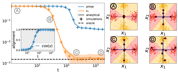
Figure 2: How the 2LNN learns a XOR-like GM (Left) Evolution of the prediction mean-squared error $\operatorname{\sf pmse}$ (8) and the classification error (2) of a 2LNN with $K=8$ neurons trained on the XOR-like mixture of Fig. 1. We plot the test errors as obtained from a single simulation with $D=1000$ (crosses) and from integration of the ODEs of Sec. 2.2. The dashed black line is the classification error of an oracle with knowledge of the means $\mu^{\alpha}$, Eq. (3). The inset shows the mean angle of the network weights to the means of the mixture. (Right) Projections of the first layer weights (dots) onto the plane spanned by the means of the XOR-like mixture at different times during training. Shaded areas indicate the decision boundaries of the network, where its output $\phi_{\theta}(x)$ changes sign. Parameters: $K=8,D=1000,\sigma=0.05,\eta=0.1$ weights initialised with s.t.d. $\sigma_{0}=1$, $\kappa=10^{-2}$.

Dynamics

We derived a closed set of ordinary differential equations that describe the evolution of the order parameters in the case where each Gaussian in the mixture has the same covariance matrix $\Omega$. We proceed here with a brief statement of the equations and deffer the detailed derivation to Sec. B.2. The approach is most easily illustrated with the second-layer weights $v^{k}$. The key idea to compute the average change in the weight $v^{k}$ upon an SGD update (7b), $\operatorname{d}\!v^{k}$, which can be decomposed into a contribution from every Gaussian in the mixture,

$$\mathbb{E}\,\operatorname{d}\!v^{k}\!=\!\sum_{\alpha\in\mathcal{S}\left(+\right)}\mathcal{P}_{\alpha}\operatorname{d}\!v^{k}_{\alpha^{+}}+\sum_{\alpha\in\mathcal{S}\left(-\right)}\mathcal{P}_{\alpha}\operatorname{d}\!v^{k}_{\alpha^{-}}\,,$$ (11)

where the change $\operatorname{d}\!v^{k}_{\alpha^{+}}$ is obtained directly from Eq. (7b),

$$\operatorname{d}\!v^{k}_{\alpha}\!=\!\frac{\eta}{D}\mathop{\mathbb{E}\,}_{\alpha}y_{\alpha}g(\lambda^{k})\!-\!\frac{\eta}{D}\sum_{j}\!v^{j}\mathop{\mathbb{E}\,}_{\alpha}g(\lambda^{k})g(\lambda^{j})\!-\!\frac{\eta}{D}\kappa v^{k}.$$ (12)

The averages that remain to be computed only involve the true label and the local fields $\lambda$. The former is a constant within each Gaussian while the latter are jointly Gaussian. It follows, that also these averages can be expressed in terms of only the order parameters and the equation closes. As we discuss in the appendix, in the high-dimensional limit $D\!\to\!\infty$ the normalised number of samples $t\!\equiv\!\nicefrac{{N}}{{D}}$ can be interpreted as a continuous time, which allows the dynamics of $v^{k}$ to be captured by the ODE (B.28).

The order parameters $Q$ require an additional step which consists in diagonalising the sum $Q^{k\ell}~{}\!\sim~{}\!\mathop{\sum}_{r,s}^{D}w^{k}_{r}\Omega_{rs}w^{\ell}_{s}$ by introducing the integral representation

$$Q^{kl}=\int\operatorname{d}\!\rho\;p_{\Omega}(\rho)\;\rho q^{kl}(\rho),\quad$$ (13)

where $p_{\Omega}(\rho)$ is the spectral density of $\Omega$, and $q^{kl}(\rho)$ is a density whose time evolution can be characterised in the thermodynamic limit. We relegate the full expression of the equation of motion for $q^{kl}(\rho)$ to Eq. (B.27) of the appendix. Crucially, it involves only averages that can be expressed in terms of the order parameters (9), and hence the equation closes. Likewise, the order parameter $M$ can be rewritten in terms of a density as $M^{\alpha k}=\int\operatorname{d}\!\rho\;p_{\Omega}(\rho)m^{\alpha k}(\rho)$. The dynamics of $m^{\alpha k}$ is described by Eq. (B.22).

Solving the equations of motion

The equations are valid for any mean and covariance matrix $\Omega$. Solving them requires evaluating multidimensional integrals of dimension up to 4, e.g. $\mathop{\mathbb{E}\,}_{\alpha}g^{\prime}(\lambda^{k})\lambda^{\ell}y$, which can be effeciently estimated using Monte-Carlo (MC) methods. We provide a ready-to-use numerical implementation on the GitHub.

Comparing theory and simulation

On the left of Fig. 2, we plot the evolution of the $\operatorname{\sf pmse}$ (8) and the classification error (2) of a 2LNN with $K=8$ neurons trained on the XOR-like mixture of Fig. 1. We plot the test errors obtained from integration of the order parameters with solid lines, and the same quantities computed using a test set during the simulation with crosses. The agreement between ODE predictions and a single run of SGD is good, even at intermediate system size ($D=1000$). In the App. B.2, we give additional plots for the simulated dynamics of the individual order parameters and find very good agreement with predictions obtained from the ODEs (cf. Fig. 7). Note that although we initialise the weights of the student randomly and independently of the means, there is an initial overlap between student weights and the means of order $1/\sqrt{D}$ due to finite-size fluctuations. To capture this with the ODEs, we initialise them in a regime of weak recovery, where $M^{k}_{\alpha}\!\neq\!0$. For a detailed discussion of the early period of learning up to weak recovery, see Arous et al. (2020).

How 2LNNs learn the XOR-like mixture

A closer look at the learning dynamics on the right of Fig. 2 reveals several phases of learning. There we show the first-layer weight vectors of the 2LNN, projected into the plane spanned by the four means of the mixture, at four different times during training. The regions shaded in red and yellow indicate the decision boundaries of the network, which correspond to the line where the network’s output $\phi_{\theta}(x)$ changes its sign. A 2LNN with $K\geq 4$ neurons can approach the classification error of the oracle (3) if its weight vectors approach the four means, with corresponding second-layer weights. Panel (C) shows that network reaches this configuration. However, this configuration does not minimise the mean-squared error used during training (7), so eventually the weights depart slightly from the means to converge to a solution with lower mean squared error (D). This is confirmed by the inset on the left of Fig. 2, where we see that the average angle of the network weights to the means has a maximum around $t=300$, before decaying slightly at the end of training.

2.3 Predicting the long-time performance of 2LNN

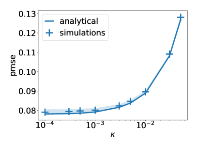
Figure 3: Prediction mean-squared error (8) on the XOR-like mixture versus weight decay. Results obtained from a fixed point analysis of the ODEs with 4 degrees of freedom discussed in Sec. 2.3 ($\sigma^{2}=0.1,K=4,\eta=0.1,10^{4}$) Monte-Carlo samples. The shaded area indicates standard deviation over 10 runs.

Direct integration of the ODEs is numerically expensive. A more straight forward way to extract information from the ODEs is to find their asymptotic fixed point, which fully characterises the $t\to\infty$ performance of the network. However, the number of equations is already 26 for a 2LNN with 4 neurons trained on the XOR mixture, and scales like $K^{2}$. The key to finding fixed points efficiently is thus to make an ansatz with fewer degrees of freedom for the matrices $Q$ and $M$ which solve the equations. For example, one could impose $Q^{kk}=Q$ and $Q^{k\ell}=C,k\neq\ell$. By exploiting the symmetries of the XOR-like mixture, we find that the fix points of the equations can be described by only $K=4$ parameters: $\nicefrac{{K}}{{2}}$ angles between weight vectors and means, and $\nicefrac{{K}}{{2}}$ norms, as described in Appendix B.3. Finding the fixed-point of this reduced four-dimensional system allows to compute, for example, the dependence of the generalisation error as a function the regularisation in Fig. 3. The agreement between simulation and analytical predictions is again good, and we find that increasing the regularisation only increases the test error of the student. This is in agreement with previous work on two-layer networks in the same limit in the teacher-student setup, where $L_{2}$-regularisation was also found to hurt performance (Saad & Solla, 1997).

Figure 4: Fraction of simulations that converged to the optimal solution for the 2LNN out of 20 simulations for increasing values of $K$. Overparametrisation increases the probability of finding the optimal solution but does not affect classification performances. Simulations started with initial weights of std.dev. $\sigma_{0}$. The inset shows the classification error of the networks that converged. Parameters: $D=800,\eta=0.1,\kappa=0,\sigma^{2}=0.1$, run time $10^{5}$.

2.4 The impact of over-parametrisation

We also studied the effect of over-parametrisation, which we define as the number of additional neurons a student has on top of the $K=4$ neurons that it needs to reach the oracle’s performance on the XOR mixture. We show in the inset of Fig. 4 that over-parametrisation does not improve final performance, since the remaining error of the student is dominated by “spill-over” of points from one mixture into adjacent quadrants. However, over-parametrisation leads to an “implicit acceleration” effect: over-parametrised networks are much more likely to converge to a solution that approaches the oracle’s performance, as we show in the main of Fig. 4. The term “implicit acceleration” was coined by Arora et al. (2018) for similar effects in deep neural networks, and analysed for two-layer networks in the teacher-student setup by Livni et al. (2014); Safran & Shamir (2018). A complete understanding of the phenomenon remains an open problem, which we leave for future work.

3 Random features on GM classification

To understand the performance of random features on Gaussian Mixtures classification, we analyse the performances of the linear model (5) trained with online SGD with the squared loss on the random features $z$ (4) (Steinwart et al., 2009; Caponnetto & De Vito, 2007).

First, we assume that we have enough samples, so that $N\gg P$, and discuss the situation when $N~{}\ll~{}P$ later. For any finite $D,P$, running the algorithm up to convergence then corresponds to taking the limit $t\to\infty$. The random features’ weights converge to an estimate $\hat{W}$ which can be computed analytically, see Eq. D.6, and allows to precisely characterise the test error:

$$\operatorname{\sf pmse}_{t\to\infty}=\frac{1}{2}\Big{(}1-\sum_{\tau}\frac{\tilde{\Phi}_{\tau}^{2}}{\rho_{\tau}}\Big{)},$$ (14)

where $\rho_{\tau}$ are the eigenvalues of the feature’s covariance matrix $\Omega_{ij}=\mathbb{E}\,z_{i}z_{j}$, with associated eigenvector $\Gamma_{\tau}$. $\tilde{\Phi}_{\tau}\!\equiv\!\sum_{i=1}^{P}\Gamma_{\tau i}\Phi_{i}/\sqrt{P}$ is the input-label covariance after rotation into the eigenbasis of $\Omega$ (see Appendix D). Crucially, the test error and $\hat{W}$ only depend on the first two moments of the features. The formula for these moments, as well as the one for the classification error can be obtained when $P,D$ are large using the Gaussian equivalence of (Goldt et al., 2020a). Indeed, the distribution of the features $z$ remains a mixture of distributions (see App. C). We then define

$$M_{\alpha}\!=\!\sum_{i=1}^{P}\frac{\hat{w}_{i}\mathop{\mathbb{E}\,}_{\alpha}[z_{i}]}{\sqrt{P}},\text{ }Q_{\alpha}\!=\!\sum_{i=1}^{P}\frac{\hat{w}_{i}\hat{w}_{j}}{P}\mathop{\operatorname{\mathsf{Cov}}}_{\alpha}(z,z),$$ (15)

and we find for $D,P$ large enough, that

$$\epsilon_{ct\to\infty}=\frac{1}{2}\left(1-\sum_{\alpha}\mathcal{P}_{\alpha}\,y\,\mathrm{erf}\left(\frac{M_{\alpha}}{\sqrt{2Q_{\alpha}}}\right)\right).$$ (16)

As discussed in App. C.3, in the case of ReLU activation function, the feature distribution $p(z_{i})$ is a truncated Gaussian. Hence, at large $D$, $P$, both the mean of $z_{i}$ and the population covariance $\operatorname{\mathsf{Cov}}(z_{i},z_{j})$ can be obtained analytically in terms of the matrix $F$ and means $\mu$, see Eq. (C.16) and (C.19) for the full result.

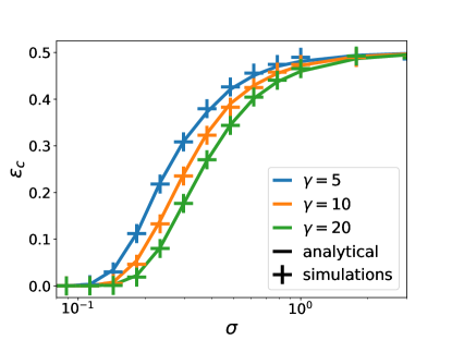
Figure 9: Agreement between analytical predictions and simulations of the classification error of RF trained on the XOR like mixture of Fig. 1 for increasing $\sigma$ and various $\gamma$. The analytical predictions are obtained by computing the moments of the features $z$ using Eq. C.16 and Eq. C.19. These are then used to obtain, first the asymptotic solution of RF via Eq. D.6, which is in turn plugged in Eq. D.9. The final result is then given by Eq. D.8. Simulation results are obtained by training online an RF network with $\eta=0.1$ until convergence. Parameters: $D=800$, $\eta=0.1$, $P=\gamma D$, $\nicefrac{{|\mu|}}{{\sqrt{D}}}=1$.

We used this formula to obtain precisely the error (14), and the results are shown in Fig. 5. We see that the RF error is a function of $\sigma D^{1/2}/P^{1/4}=\sigma(\nicefrac{{D}}{{\gamma}})^{1/4}$ leading to the conclusion that – as discussed in Fig. 1 – the “transition” from the high to low $\operatorname{\sf snr}$ regime happens when $\sigma^{-1}~{}\approx~{}\nicefrac{{{D}^{1/2}}}{{P^{1/4}}}$. This scaling further reveals that $P\approx D^{2}$ features are required in order to obtain good performance. The validity of Eq. 16 is verified in Fig. 9. Reaching this performance, however, requires the number of samples $N$ to be larger than $P$, so $N>O(D^{2})$. In the so-called high-dimensional regime analysed in this paper, where $N\approx D$, such performances remain out of reach. The scaling analysis can be easily generalised; as discussed by Ghorbani et al. (2019); Mei et al. (2021), the relevant dimension for RF performances is, rather than $P$, the minimum between $N$ and $P$.

The classification error is thus a function of $\sigma\nicefrac{{D^{1/2}}}{{\min(N,P)}}^{1/4}$. If $N$ is $O(D)$, then even in the kernel limit when $P\to\infty$, the performance degrades to no more than a random guess as soon as

$$\sigma\gg\nicefrac{{N^{1/4}}}{{D^{1/2}}},$$ (17)

and therefore for any value of $\sigma$ when $D,N\to\infty$ with fixed $N/D$. In a nutshell, for any fixed $\sigma$, lazy training methods such as random features or kernels will fail to beat a random guess in the high-dimensional limit. This, and the requirement of at least $N=O(D^{2})$ samples to learn, are to be contrasted with the the oracle-like performance achieved by a simple neural net with only $N=O(D)$ samples.

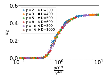
Figure 5: Evolution of the classification error of random features (RF) for various values of $\sigma$, $\gamma=P/D$ and $D$ on the XOR mixture of Fig. 1, in the limit of large number of samples $N\gg P$. All these different cases can be collapsed into a single master curve by plotting the classification error versus $\sigma D^{1/2}/P^{1/4}=\sigma D^{1/4}/\gamma^{1/4}$, showing that for large $D,P$, it should be a function $\epsilon_{c}=f(\sigma D^{1/2}/P^{1/4})$. For a finite input dimension $D$, increasing the number of features allows RF to perform increasingly better as they approach the Kernel limit. Analytical predictions are obtained by the linear regression analysis of Eq. (16) for RF. Parameters: $\eta=0.1$, $\nicefrac{{|\mu|}}{{\sqrt{D}}}=1$. Note however that this analysis requires $N\gg P$. Given random features are sensitive to the minimum of $P$ and $N$ (Ghorbani et al., 2019; Mei et al., 2021) the effective scaling variable is rather $\sigma D^{1/2}/\min(P,N)^{1/4}$ (see text).

Why do random features fail? The linear regime of features maps

This raises the question of why the random feature and kernel methods fail in the high-dimensional setting. As we shall see – and this has been already discussed in different contexts by El Karoui (2010); Mei & Montanari (2019) – this can be understood analytically from the fact that the feature map is effectively linear when when $P=O(D)$. This section is now dedicated to computing the moments $\mathop{\mathbb{E}\,}_{\alpha}[z_{i}]$ and $\mathop{\operatorname{\mathsf{Cov}}}_{\alpha}(z,z)$ analytically in this region, revealing that this effective linearity is indeed the underlying reason for the failure of RF in this regime.

Since the mixture remains a mixture after the application of random features, our main task is to compute the new means and variances of the distribution in the transformed space. We thus focus on transformation of a random variable drawn from a single Gaussian $x_{r}=\mu_{r}/\sqrt{D}+\sigma w_{r}$, where $w_{r}$ is a standard Gaussian, in the kernel, or random feature, space.

For generic activation function the first two moments of the features can be obtained in the well studied low signal-to-noise regime $\operatorname{\sf snr}\sim O(1)$. Key to do so, is the observation that $\nicefrac{{F_{ir}\mu_{r}}}{{D}}\sim O(\nicefrac{{1}}{{\sqrt{D}}})$. The activation function can thus be expanded in orders of $\nicefrac{{1}}{{D}}$ and its action is essentially linear. We define the constants

$$a\equiv\mathbb{E}\,\psi\left(\sigma\zeta\right),\quad b\equiv\mathbb{E}\,\zeta\psi\left(\sigma\zeta\right),\quad c^{2}\equiv\mathbb{E}\,\psi\left(\sigma\zeta\right)^{2}$$ (18)

with the expectation taken over the standard Gaussian random variable $\zeta$. To leading order, the mean and covariance of the features are given by (cf. Sec. C):

$$\mathbb{E}\,z_{i} =a+b\sum_{r=1}^{D}\frac{F_{ir}\mu_{r}}{\sigma D}\,$$ (19)

$$\operatorname{cov}(z_{i},z_{j}) =\begin{cases}c^{2}-a^{2},\quad&i=j\,,\\ b^{2}\sum_{r}\frac{F_{ir}F_{jr}}{D}\quad&i\neq j.\end{cases}$$ (20)

This computation immediately reveals the reason random features cannot hope to learn in the low $\operatorname{\sf snr}$ regime: the transformation of the means is only linear; hence a Gaussian mixture that is not linearly separable in input space will remain so even after random features. In other words, if the centres of the Gaussian are too close, the kernel fails to map the data non-linearly to a large dimensional space. In contrast, in the high-$\operatorname{\sf snr}$ regime, where the centres are separated enough, the non-linearity kicks-in and the data becomes separable in feature space.

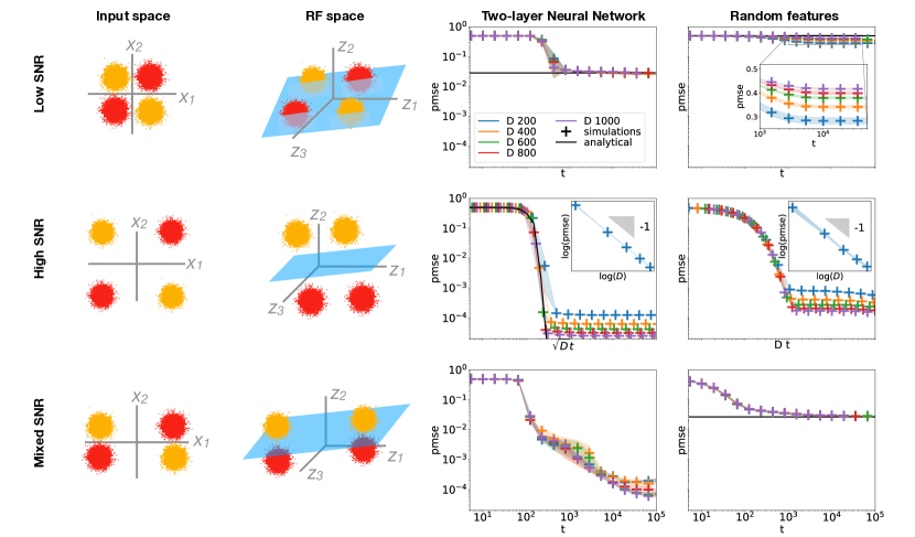
Figure 6: The performance of 2LNN and RF on the XOR-like mixture with different signal-to-noise ratios. The first and second columns show the XOR-like mixture in input space and random feature space, resp. The third and fourth columns show the $\operatorname{\sf pmse}$ (8) of 2LNN and RF during training, resp. In the low $\operatorname{\sf snr}$ regime (top row), while the 2LNN learns a non trivial function of the inputs, RF cannot perform better than random chance since the XOR-like mixture remains one in feature space. Both networks learn to classify the XOR-mixture in the high $\operatorname{\sf snr}$ regime (middle row) as the clusters become well separated in feature space. For mixed $\operatorname{\sf snr}$ (bottom row), even though both networks do better than random guessing, 2LNN outperform RF as the distance between opposite sign clusters remains of order one in feature space. In all plots, crosses are obtained from simulations with input dimension $D=1000$. Solid black lines in the 2LNN plots are obtained using tools from Sec. 2.2 (long-time performance of Sec. 2.3 for the first row and integration of the odes for the second). Solid black lines in the RF plots indicate the test error obtained from the analysis of Sec. 3 with $D=10000$. $\sigma^{2}=0.05,P=2D,\eta=0.1,K=10,\sigma_{0}=10^{-2}$.

Relation to kernel methods

The same argument explains the failure of kernel methods: if two centres $\bf x$ and $\bf y$ are close, the kernel function $K({\bf x},{\bf y})$ can be expanded to low order and the kernel is essentially linear, leading to bad performances. The connection can be made explicit using the convergence of random features to a kernel (Rahimi & Recht, 2008, 2009):

$$K(\bm{x},\bm{y})\!=\!\frac{1}{P}\!\sum_{i=1}^{P}\mathop{\mathbb{E}\,}_{F}\!\left[\psi\left(\sum_{r=1}^{D}\frac{x_{r}F_{ir}}{\sqrt{D}}\right)\psi\left(\sum_{s=1}^{D}\frac{y_{s}F_{is}}{\sqrt{D}}\right)\right],$$ (21)

At low SNR, the constants $a,b,c$ can be obtained from the kernel via

$$\begin{aligned} c^{2}=\mathbb{E}\,K(\sigma\bm{\omega}_{1},\sigma\bm{\omega}_{1}),\quad a^{2}=\mathbb{E}\,K(\sigma\bm{\omega}_{1},\sigma\bm{\omega}_{2}),\\ b^{2}=D\sigma^{2}\left[-a^{2}+\mathbb{E}\,K\left(\frac{\bm{\mu}}{\sqrt{D}}+\sigma\bm{\omega}_{1},\frac{\bm{\mu}}{\sqrt{D}}+\sigma\bm{\omega}_{2}\right)\right]\end{aligned}$$

where the average is taken over two standard Gaussian random vectors $\omega_{1},\omega_{2}\in\mathbb{R}^{D}$. This relation, similar in nature to one of El Karoui (2010), allows to express the statistical properties of the features directly from the kernel function.

4 Neural networks vs random features

We now collect our results for a comparison of the performance of 2LNN and RF on the XOR-like mixture from Fig. 1. We look at three different regimes for the $\operatorname{\sf snr}$, illustrated in the first column of Fig. 6. The second column visualises the mixture after the Gaussian random features transformation with $\psi(x)=\max(0,x)$ (4). The third and fourth columns show the evolution of the $\operatorname{\sf pmse}$ of 2LNN and RF, respectively, during training with online SGD. Since overparametrisation does not impact the 2LNN’s performance in these tasks, Sec. 2.3, we train a $K=10$ network to increase the number of runs that converge.

At low $\operatorname{\sf snr}$ (a) the distance of each Gaussian to the origin is $O(1)$ and the standard deviation $\sigma\sim O(1)$ as well. The two-layer neural network learns to predict the correct labels almost as well as the oracle (3). Its performance does not depend on $D$, and using the long-time solution of Sec. 2.3, we can predict its asymptotic error (black line) which agrees well with simulations (crosses). In contrast, random features display an asymptotic error that approaches random guessing as the input dimensions increases (inset). This is clear from Eq. 20: in the large $D$ limit, random features only produce a linear transformation of their input. The XOR therefore remains a XOR in RF space, leading linear regression’s failure to do better than chance.

At high $\operatorname{\sf snr}$ (b), the distance between the clusters scales as $\sqrt{D}$ while the $\sigma$ remains fixed. The asymptotic error of the 2LNN thus decreases with $D$ and the network is able to learn perfectly in the $D\to\infty$ limit (black line). The error of random features also approaches 0 as $D\to\infty$, since the mixture is now well separated in random feature space, too.

We finally consider a regime of mixed $\operatorname{\sf snr}$ (c) where the mixture is well-separated in one dimension, but very close in the other dimension. We achieve this by setting $\mu^{0}_{1}\!~{}\sim~{}\!\sqrt{D},\mu^{0}_{2}~{}\!\sim\!~{}D$ for the mean of the first mixture, etc. Random features then achieve a non-trivial generalisation error, which can be understood by considering the means of the features $z_{i}$. The large component $\mu_{2}$, induces the activation function to perform a non-linear transformation of the centres and allows for opposite sign centroids to be separated by a hyper-plane in feature space. The small component $\mu_{1}$, causes the distance between opposite sign centroids, which is of order $O(1)$ in input space, to remain of order one in feature space, for all $D$. This leads to a finite generalisation error of RF which remains invariant with increasing input dimension. In this regime, the 2LNN still achieve better performance than the random features, thereby completing the picture we developed in Fig. 1.

Appendix A Summary of Notations

$D$	input dimensions	$P$	number of random features
$N$	number of samples	$\gamma=\nicefrac{{P}}{{D}}$
$t=\nicefrac{{N}}{{D}}$	training time, or equivalently rescaled number of training samples	$y$	true label
$\Omega^{\alpha}\in\mathbb{R}^{D\crossproduct D}$	covariance of the normal distribution of cluster $\alpha$	$\frac{\mu^{\alpha}}{\sqrt{D}}\in\mathbb{R}^{D}$	mean of the Gaussian cluster $\alpha$ in the mixture
$x\in\mathbb{R}^{D}$	input	$\sigma$	standard deviation of the Gaussian clusters in a mixture with $\Omega_{\alpha}=\sigma^{2}\mathbb{I}$
$\operatorname{\sf snr}\!=\!\frac{|\mu|}{\sigma\sqrt{D}}$	signal to noise ration	$\eta$	learning rate
$\kappa$	$L2$-regularisation constant	$\operatorname{\sf pmse}$	population mean squared error
$\epsilon_{c}$	classification error

$\text{ }q(x|y)\!=\!\!\sum\limits_{\alpha\in\mathcal{S}(y)}\!P_{\alpha^{\pm}}\mathcal{N}_{\alpha}(x)$ conditional probability of $x$ given the true label $y$

Two layer neural networks (2LNN)

$K$	number of hidden nodes of the 2LNN	$w_{i}^{k}$	first layer weights
$v^{k}$	second layer weights	$g:\mathbb{R}\to\mathbb{R}$	activation function
$\lambda\equiv\sum\limits_{r}\nicefrac{{w_{r}^{k}x_{r}}}{{\sqrt{D}}}$	local field/pre-activation of the 2LNN	$\phi(\theta)=\sum\limits_{k=1}^{K}v^{k}g(\lambda^{k})$	output of the network
$Q_{\alpha}^{kl}\!=\!\sum\limits_{rs}\frac{w^{k}_{r}\Omega^{\alpha}_{rs}w^{l}_{s}}{D}$	order parameter/ covariance of the local fields	$M_{\alpha}^{k}\!=\!\sum\limits_{r}\frac{w^{k}_{r}\mu_{r}^{\alpha}}{D}$	order parameter/mean of the local fields
$\sigma_{0}$	weights are initialised i.i.d. from $\mathcal{N}(0,\sigma_{0}^{2})$

Random Features (RF)

$F\in\mathbb{R}^{P\times D}$	projection matrix     $F_{ir}\!\overset{\text{i.i.d.}}{\sim}\!\mathcal{N}(0,1)$	$z\equiv\psi\left(\sum\limits_{r=1}^{D}\nicefrac{{F_{ir}x_{r}}}{{\sqrt{D}}}\right)$	features
$\psi:\mathbb{R}\to\mathbb{R}$	activation function applied element wise	$\phi(\theta)=\sum\limits_{i=1}^{P}\nicefrac{{w_{i}z_{i}}}{{\sqrt{D}}}$	output of the network
$\hat{W}$	fix point solution of the SGD update equation of RF

Appendix B Derivation of the dynamical equations

In this appendix, we derive the dynamical equations that describe the dynamics of two-layer neural networks trained on the Gaussian mixture from Sec. 2.2. We first derive a useful Lemma for the averages of weakly correlated random variables B.1, which we we then use in the derivation of the dynamical equations B.2

B.1 Moments of functions of weakly correlated variables

Here, we show how to compute expectation of functions of weakly correlated variables with non zero mean. The derivation follows the ones of (Goldt et al., 2020b) (see App. A). We extend their computations to include variables with non-zero means.

Consider the random variables $x$,$y\in\mathbb{R}$, jointly Gaussian with joint probability distribution:

$$P(x,y)=\frac{1}{2\pi\sqrt{\det M_{2}}}\exp\left[-\frac{1}{2}\left(\begin{array}[]{ll}x-\bar{x}&y-\bar{y}\end{array}\right)M_{2}^{-1}\left(\begin{array}[]{l}x-\bar{x}\\ y-\bar{y}\end{array}\right)\right],$$ (B.1)

where we defined the mean of $x$, respectively $y$, as $\bar{x}$, respectively $\bar{y}$ and the covariance matrix:

$$M_{2}=\left(\begin{array}[]{ll}C_{x}&\epsilon M_{12}\\ \epsilon M_{12}&C_{y}\end{array}\right).$$ (B.4)

The weak correlation between $x$ and $y$ is encapsulated in the parameter $\epsilon\ll 1$ while $M_{12}\!\sim\!O(1)$.

We are interested in computing expectations of the form $\displaystyle\mathop{\mathbb{E}\,}_{(x,y)}[f(x)g(y)]$ with two real valued functions $f,g:\mathbb{R}\to\mathbb{R}$. Leveraging the weak correlation between $x$ and $y$, we can expand the distribution Eq. (B.1) to linear order in $\epsilon$, i.e.:

$$(\eqref{eq:joint_gaussian})=\frac{1}{2\pi\sqrt{C_{x}C_{y}}}\operatorname{e}^{-\frac{1}{2C_{x}}(x-\bar{x})^{2}-\frac{1}{2C_{y}}(y-\bar{y})^{2}}{\left[1-\epsilon(x-\bar{x})\left(C_{x}^{-1}M_{12}C_{y}^{-1}\right)(y-\bar{y})+O\left(\epsilon^{2}\right)\right]}$$ (B.5)

Using the above, one can compute the expectations:

$$\mathop{\mathbb{E}\,}_{(x,y)}\left[f(x)g(y)\right]= \mathop{\mathbb{E}\,}_{x}\left[f(x)\right]\mathop{\mathbb{E}\,}_{y}\left[g(y)\right]$$

$$+\epsilon\mathop{\mathbb{E}\,}_{x}\left[f(x)(x-\bar{x})\right]\left(C_{x}^{-1}M_{12}C_{y}^{-1}\right)\mathop{\mathbb{E}\,}_{y}\left[g(y)(y-\bar{y})\right]+O(\epsilon^{2}).$$ (B.6)

The expectations are now taken over the 1-dimensional distributions of $x\!\sim\!\mathcal{N}(0,C_{x})$ and $y\!\sim\!\mathcal{N}(0,C_{x})$.

Similarly, consider the case of three weakly correlated real random variables $x_{i}$, $i=1,2,3$ with mean $\bar{x}_{i}$ and covariance matrix $M_{3}$ such that

$$(M_{3})_{ij}=\begin{cases}C_{i},\text{ if }i=j\\ \epsilon M_{ij},\text{ if }i\neq j\end{cases}.$$ (B.7)

One can use an expansion of the joint probability distribution of $\{x_{i}\}$ to linear order in $\epsilon$ to compute three point moments of real valued functions $f,g,h$ as:

$$\mathop{\mathbb{E}\,}_{\{x\}_{i}}\left[f(x_{1})g(x_{2})h(x_{3})\right]= \mathop{\mathbb{E}\,}_{\{x\}_{i}}\left[f(x_{1})\right]\left[g(x_{2})\right]\left[h(x_{3})\right]$$

$$-\epsilon\mathop{\mathbb{E}\,}_{x_{3}}[h(x_{3})]\mathop{\mathbb{E}\,}_{x_{1}}[(x_{1}-\bar{x}_{1})f(x_{1})]\left(C_{x}^{-1}M_{12}C_{y}^{-1}\right)\mathop{\mathbb{E}\,}_{x_{2}}[(x_{2}-\bar{x}_{2})g(x_{2})]$$

$$-\epsilon\mathop{\mathbb{E}\,}_{x_{2}}[g(x_{2})]\mathop{\mathbb{E}\,}_{x_{1}}[(x_{1}-\bar{x}_{1})f(x_{1})]\left(C_{x}^{-1}M_{13}C_{y}^{-1}\right)\mathop{\mathbb{E}\,}_{x_{3}}[(x_{3}-\bar{x}_{3})h(x_{3})]$$

$$-\epsilon\mathop{\mathbb{E}\,}_{x_{1}}[f(x_{1})]\mathop{\mathbb{E}\,}_{x_{2}}[(x_{2}-\bar{x}_{2})g(x_{2})]\left(C_{x}^{-1}M_{23}C_{y}^{-1}\right)\mathop{\mathbb{E}\,}_{x_{3}}[(x_{3}-\bar{x}_{3})h(x_{3})]+O(\epsilon^{2}).$$ (B.8)

In the case in which $x_{1}$ and $x_{2}$ are weakly correlated with $x_{3}$ but not between each other, i.e. $\operatorname{Cov}(x_{1},x_{2})=M_{12}\!\sim\!O(1)$, one has:

$$\begin{split}\mathbb{E}\,\left[f(x_{1})g(x_{2})h(x_{3})\right]=&\mathbb{E}\,\left[f(x_{1})g(x_{2})\right]\mathbb{E}\,\left[h(x_{3})\right]\\ &+\epsilon\frac{\mathbb{E}\,\left[h(x_{3})(x_{3}-\bar{x}_{3})\right]}{\left(C_{x_{1}}C_{x_{2}}-M_{12}^{2}\right)C_{x_{3}}}\left\{\mathbb{E}\,\left[f(x_{1})g(x_{2})(x_{1}-\bar{x}_{1})\right]M_{13}C_{x_{2}}\right.\\ &\hskip 110.00017pt\left.+\mathbb{E}\,\left[f(x_{1})g(x_{2})(x_{2}-\bar{x}_{2})\right]M_{23}C_{x_{1}}\right.\\ &\hskip 110.00017pt\left.-\mathbb{E}\,\left[f(x_{1})g(x_{2})(x_{1}-\bar{x}_{1})\right]M_{12}M_{23}\right.\\ &\hskip 110.00017pt\left.-\mathbb{E}\,\left[f(x_{1})g(x_{2})(x_{2}-\bar{x}_{2})\right]M_{13}M_{12}\right\}+O(\epsilon^{2}).\end{split}$$ (B.9)

B.2 Derivation of the ODEs

In this section, we derive the ODEs describing the dynamics of training of a 2LNN trained on inputs sampled from the distribution (6) with $L2$-regularisation constant $\kappa$. We restrict to the case where all the Gaussian clusters have the same covariance matrix, i.e. $\Omega^{\alpha}=\Omega\in\mathbb{R}^{D\crossproduct D}$.

In order to track the training dynamics, we analyse the evolution of the macroscopic operators defined in Eq. (9) allowing to compute the performances of the network at all training times.

At the $s$th step of training, the SGD update for the networks parameter is given by Eq. (7):

$$\operatorname{d}\!w_{i}^{k}\equiv\left(w_{i}^{k}\right)_{s+1}-\left(w_{i}^{k}\right)_{s}=-\frac{\eta_{W}}{\sqrt{D}}\left(v^{k}\Delta g^{\prime}(\lambda^{k})x_{i}+\kappa w^{k}_{i}\right),\qquad\operatorname{d}\!v^{k}=-\frac{\eta_{v}}{\sqrt{D}}\left(g(\lambda^{k})+\kappa v^{k}\Delta\right).$$ (B.10)

In order to guarantee that the dynamics can be described by a set of ordinary equations in the $D\to\infty$ limit, we choose different scalings for the first and second layer learning rates:

$$\eta_{W}=\eta,\qquad\eta_{v}=\eta/D$$

for some constant $\eta$.

Update of the first layer weights

To make progress, consider the eigen-decomposition of the covariance matrix:

$$\Omega_{rs} =\frac{1}{D}\sum_{\tau=1}^{D}\Gamma_{s\tau}\Gamma_{r\tau}\rho_{\tau};$$ (B.11)

where we denote the eigenvalues as $\rho_{\tau}$, their corresponding eigenvector as $\Gamma_{\tau}$ and the eigenvalue distribution as $p_{\Omega}$. We further define the projection of the weights into the projected basis as

$$\tilde{w}_{\tau}^{k}\equiv\frac{1}{\sqrt{D}}\sum_{\tau=1}^{D}\Gamma_{s\tau}w^{k}_{s}$$ (B.12)

and similarly $\tilde{x}_{\tau}$ and $\tilde{\mu}^{\alpha}_{\tau}$ as the projected inputs and means. In this basis, the SGD update for the first layer weights is:

$$\operatorname{d}\!\tilde{w}_{\tau}^{k}\equiv\left(\tilde{w}_{\tau}^{k}\right)_{s+1}-\left(\tilde{w}_{\tau}^{k}\right)_{s}=-\frac{\eta}{\sqrt{D}}\left(v^{k}\Delta g^{\prime}(\lambda^{k})\tilde{x}_{\tau}+\kappa w_{\tau}^{k}\right).$$ (B.13)

The expectation of this update over the distribution Eq. (6) is given by:

$$\mathbb{E}\,\operatorname{d}\!\tilde{w}_{\tau}^{k}=\sum_{\alpha\in\mathcal{S}\left(+\right)}\mathcal{P}_{\alpha}\operatorname{d}\!\tilde{w}^{k}(\rho)_{\alpha^{+}}+\sum_{\alpha\in\mathcal{S}\left(-\right)}\mathcal{P}_{\alpha}\operatorname{d}\!\tilde{w}^{k}(\rho)_{\alpha^{-}},$$ (B.14)

where we decomposed the expectation into the different clusters and introduced:

$$\operatorname{d}\!\tilde{w}^{k}(\rho)_{\alpha^{\pm}}= \pm\frac{\eta}{\sqrt{D}}v^{k}\mathcal{C}^{k}_{\tau}-\frac{\eta}{\sqrt{D}}\sum_{j\neq k}v^{k}v^{j}\mathcal{A}^{kj}_{\tau}-\frac{\eta}{\sqrt{D}}v^{k}v^{k}\mathcal{B}^{k}_{\tau}-\frac{\eta\kappa}{\sqrt{D}}\tilde{w}^{k}(\rho),$$ (B.15)

with the expectations $\mathcal{A}^{kj}_{\tau},\mathcal{B}^{k}_{\tau}$ and $\mathcal{C}^{k}_{\tau}$ defined as:

$$\mathcal{A}^{kj}_{\tau}=\mathop{\mathbb{E}\,}_{\alpha}g^{\prime}(\lambda^{k})g(\lambda^{j})\tilde{x}_{\tau},\quad\mathcal{B}^{k}_{\tau}=\mathop{\mathbb{E}\,}_{\alpha}g^{\prime}(\lambda^{k})g(\lambda^{k})\tilde{x}_{\tau},\quad\mathcal{C}^{k}_{\tau}=\mathop{\mathbb{E}\,}_{\alpha}g^{\prime}(\lambda^{k})\tilde{x}_{\tau}.$$ (B.16)

A crucial observation, is that $\lambda^{k}$ and the projected input $\tilde{x}_{\tau}$ are jointly Gaussian and weakly correlated, with a correlation of order $1/\sqrt{D}$:

$$\mathop{\mathbb{E}\,}_{\alpha}\lambda^{k}\tilde{x}_{\tau}=\frac{1}{\sqrt{D}}\rho_{\tau}\tilde{w}^{k}.$$ (B.17)

Thus, we can compute the expressions Eq. (B.16) using the proposition for weakly correlated variables derived in App. B.1. This gives:

$$.\begin{split}\mathcal{A}^{kj}_{\tau}&=\mathop{\mathbb{E}\,}_{\alpha}g^{\prime}(\lambda^{k})g(\lambda^{j})\frac{\tilde{\mu}^{\alpha}_{\tau}}{\sqrt{D}}\\ &\quad+\frac{1}{Q^{kk}Q^{jj}-Q^{kj2}}\left\{\left(\mathop{\mathbb{E}\,}_{\alpha}g^{\prime}(\lambda^{k})\lambda^{k}g(\lambda^{j})-\mathop{\mathbb{E}\,}_{\alpha}g^{\prime}(\lambda^{k})g(\lambda^{j})M^{\alpha k}\right)\left(Q^{jj}\frac{\tilde{w}^{k}_{\tau}\rho_{\tau}}{\sqrt{D}}-Q^{kj}\frac{\tilde{w}^{j}_{\tau}\rho_{\tau}}{\sqrt{D}}\right)\right.\\ &\hskip 100.00015pt\left.\left(\mathop{\mathbb{E}\,}_{\alpha}g^{\prime}(\lambda^{k})\lambda^{j}g(\lambda^{j})-\mathop{\mathbb{E}\,}_{\alpha}g^{\prime}(\lambda^{k})g(\lambda^{j})M^{\alpha j}\right)\left(Q^{kk}\frac{\tilde{w}^{j}_{\tau}\rho_{\tau}}{\sqrt{D}}-Q^{kj}\frac{\tilde{w}^{k}_{\tau}\rho_{\tau}}{\sqrt{D}}\right)\right\}\\ \mathcal{B}^{k}_{\tau}&=\mathop{\mathbb{E}\,}_{\alpha}g^{\prime}(\lambda^{k})g(\lambda^{k})\frac{\tilde{\mu}^{\alpha}_{\tau}}{\sqrt{D}}+\frac{1}{Q^{kk}}\left(\mathop{\mathbb{E}\,}_{\alpha}g^{\prime}(\lambda^{k})\lambda^{k}g(\lambda^{k})-\mathop{\mathbb{E}\,}_{\alpha}g^{\prime}(\lambda^{k})g(\lambda^{k})M^{\alpha k}\right)\frac{\tilde{w}^{k}_{\tau}\rho_{\tau}}{\sqrt{D}},\\ \mathcal{C}^{k}_{\tau}&=\mathop{\mathbb{E}\,}_{\alpha}g^{\prime}(\lambda^{k})\frac{\tilde{\mu}^{\alpha}_{\tau}}{\sqrt{D}}+\frac{1}{Q^{kk}}\left(\mathop{\mathbb{E}\,}_{\alpha}g^{\prime}(\lambda^{k})\lambda^{k}-\mathop{\mathbb{E}\,}_{\alpha}g^{\prime}(\lambda^{k})M^{\alpha k}\right)\frac{\tilde{w}^{k}_{\tau}\rho_{\tau}}{\sqrt{D}},\end{split}$$ (B.18)

where we used that the first moments of the local fields are given by the order parameters, $\mathop{\mathbb{E}\,}_{\alpha}[\lambda^{k}]=M^{\alpha k}$ and $\operatorname{\mathsf{Cov}}(\lambda^{k},\lambda^{l})=Q^{kl}$. The multi-dimensional integrals of the activation function only depend on the order parameters at the previous step. We discuss how to obtain them, using monte-carlo methods in Sec 2.2. The averaged update of the first layer weights follows directly from Eq. (B.18).

Update of the Order parameters

In order to derive the update equations for the order parameters, we introduce the densities $m(\rho,t)$ and $q(\rho,t)$. These depend on $\rho$ and on the normalised number of steps $t=\nicefrac{{\mu}}{{D}}$, which we interpret as a continuous time variable.

$$m^{\alpha k}(\rho,t)=\frac{1}{D\epsilon_{\rho}}\sum_{\tau}\tilde{w}_{\tau}^{k}\tilde{\mu}_{\tau}^{\alpha}\mathbbm{1}_{\left(\rho_{\tau}\in\mathopen{[}\rho,\rho+\varepsilon_{\rho}\mathclose{[}\right)},$$

$$q^{kl}(\rho,t)=\frac{1}{D\varepsilon_{\rho}}\sum_{\tau}\tilde{w}_{\tau}^{k}\tilde{w}_{\tau}^{l}\mathbbm{1}_{\left(\rho_{\tau}\in\mathopen{[}\rho,\rho+\varepsilon_{\rho}\mathclose{[}\right)},$$ (B.19)

where $\mathbbm{1}(.)$ is the indicator function and the limit $\epsilon_{\rho}\to 0$ is taken after the thermodynamic limit. Using these definitions, the order parameters can be written as:

$$Q^{kl}(t)=\int\operatorname{d}\!\rho\;p_{\Omega}(\rho)\;\rho q^{kl}(\rho,t),\quad M^{\alpha k}(t)=\int\operatorname{d}\!\rho\;p_{\Omega}(\rho)m^{\alpha k}(\rho,t).$$ (B.20)

The equation of motion of $m$ can can be easily computed using the update (B.15) and is given by:

$$\frac{\partial m^{\beta k}(\rho,t)}{\partial t}=\sum_{\alpha\in\mathcal{S}\left(+\right)}\mathcal{P}_{\alpha}\frac{\partial m_{\alpha^{+}}^{\beta k}(\rho,t)}{\partial t}+\sum_{\alpha\in\mathcal{S}\left(-\right)}\mathcal{P}_{\alpha}\frac{\partial m_{\alpha^{-}}^{\beta k}(\rho,t)}{\partial t},$$ (B.21)

with

$$\begin{split}\frac{\partial m^{\beta k}_{\alpha^{\pm}}(\rho,t)}{\partial t}=&\pm\eta v^{k}I_{31}(k)T^{\alpha\beta}\pm\frac{\eta\rho v^{k}}{Q^{kk}}\left(I_{32}(k,k)-I_{31}(k)M^{\alpha k}\right)m^{\beta k}(\rho,t)\\ &+\sum_{j\neq k}\left[-\eta v^{k}v^{j}I_{22}(k,j)T^{\alpha\beta}\right.\\ &\qquad\quad+\frac{\eta\rho v^{k}v^{j}}{Q^{kk}Q^{jj}-Q^{kj2}}\left\{\left(-I_{3}(k,k,j)+I_{32}(k,j)M^{\alpha k}\right)\left(Q^{jj}m^{\beta k}(\rho,t)-Q^{kj}m^{\beta j}(\rho,t)\right)\right.\\ &\hskip 120.00018pt+\left.\left.\!\!\left(-I_{3}(k,j,j)+I_{32}(k,j)M^{\alpha j}\right)\left(Q^{kk}m^{\beta j}(\rho,t)-Q^{kj}m^{\beta k}(\rho,t)\right)\right\}\right]\\ &-\eta v^{k}v^{k}I_{22}(k,k)T^{\alpha\beta}-\frac{\eta\rho v^{k}v^{k}}{Q^{kk}}\left(I_{3}(k,k,k)-I_{22}(k,k)M^{\alpha k}\right)m^{\beta k}(\rho,t)-\kappa\eta m^{\beta k}(\rho,t).\end{split}$$ (B.22)

Note how, in order to close the equation, we introduced an additional order parameter $T^{\alpha\beta}=\sum_{r=1}^{D}\frac{\mu^{\alpha}_{r}\mu^{\beta}_{r}}{D}$, which is entirely defined by the overlap of the means of the mixture under consideration and is therefore a constant of motion. For compactness, we defined the multidimensional integrals $I$ of the activation function over the local fields as:

$$I_{3}(k,j,l) =\mathop{\mathbb{E}\,}_{\alpha}g^{\prime}(\lambda^{k})\lambda^{k}(\lambda^{j})$$ (B.23a)

$$I_{32}(k,j) =\mathop{\mathbb{E}\,}_{\alpha}g^{\prime}(\lambda^{k})\lambda^{j}$$ (B.23b)

$$I_{31}(k) =\mathop{\mathbb{E}\,}_{\alpha}g^{\prime}(\lambda^{k})$$ (B.23c)

$$I_{22}(k,j) =\mathop{\mathbb{E}\,}_{\alpha}g^{\prime}(\lambda^{k})g(\lambda^{j}).$$ (B.23d)

The update of $q$ can similarly be decomposed as a sum over the different Gaussian clusters:

$$\frac{\partial q^{kl}(\rho,t)}{\partial t}=\sum_{\alpha\in\mathcal{S}\left(+\right)}\mathcal{P}_{\alpha}\frac{\partial q_{\alpha^{+}}^{kl}(\rho,t)}{\partial t}+\sum_{\alpha\in\mathcal{S}\left(-\right)}\mathcal{P}_{\alpha}\frac{\partial q_{\alpha^{-}}^{kl}(\rho,t)}{\partial t}$$ (B.24)

The linear contribution to this update is directly computed by using Eq. (B.15) and is similar to the one for $m^{\beta k}(\rho,t)$. The quadratic contribution is obtained by using the fact that the projected inputs $\tilde{x}_{\tau}$ have a correlation of order $\nicefrac{{1}}{{\sqrt{D}}}$ with the local fields. Therefore, to leading order, this contribution is given by terms of the form:

$$\frac{\eta^{2}}{D^{2}}\sum_{\tau}\rho_{\tau}\mathop{\mathbb{E}\,}_{\alpha}\left[g^{\prime}(\lambda^{k})g^{\prime}(\lambda^{l})g(\lambda^{i})g(\lambda^{j})\tilde{x}^{2}_{\tau}\right]=\frac{\eta^{2}}{D}\mathop{\mathbb{E}\,}_{\alpha}\left[g^{\prime}(\lambda^{k})g^{\prime}(\lambda^{l})g(\lambda^{i})g(\lambda^{j})\right]\left(\sum_{\tau}\rho_{\tau}\mathop{\mathbb{E}\,}_{\alpha}\left[\tilde{x}^{2}_{\tau}\right]\right)+O(D^{-3/2})$$ (B.25)

Let us define the constant of motion $\chi^{\alpha}=\frac{1}{D}\sum_{\tau}\rho_{\tau}^{2}$, then the quadratic term in the update for $q_{\alpha^{\pm}}$ is given by:

$$\eta^{2}\chi^{\alpha}v^{k}v^{l}\left(I_{42}(k,l)\mp 2\sum_{j}v^{j}I_{43}(k,l,j)+\sum_{ja}v^{j}v^{a}I_{4}(k,l,j,a)\right).$$ (B.26)

The multidimensional integrals $I$ are given by:

$$I_{4}(k,l,j,a)=\mathop{\mathbb{E}\,}_{\alpha}g^{\prime}(\lambda^{k})g^{\prime}(\lambda^{l})g(\lambda^{j})g(\lambda^{a})\quad I_{43}(k,l,j)=\mathop{\mathbb{E}\,}_{\alpha}g^{\prime}(\lambda^{k})g^{\prime}(\lambda^{l})g(\lambda^{j})\quad I_{42}(k,l)=\mathop{\mathbb{E}\,}_{\alpha}g^{\prime}(\lambda^{k})g^{\prime}(\lambda^{l}).$$

Finally, the full equation of motion of $q$ is written:

$$\begin{split}\frac{\partial q^{kl}(\rho,t)_{\alpha^{\pm}}}{\partial t}=&\pm\eta v^{k}I_{31}(k)m^{\alpha k}(\rho,t)\pm\frac{\eta\rho v^{k}}{Q^{kk}}\left(I_{32}(k,k)-I_{31}(k)M^{\alpha k}\right)q^{kl}(\rho,t)\\ &+\sum_{j\neq k}\left[-\eta v^{k}v^{j}I_{22}(k,j)m^{\alpha k}(\rho,t)\right.\\ &\qquad+\left.\frac{\eta\rho v^{k}v^{j}}{Q^{kk}Q^{jj}-Q^{kj2}}\left\{\left(-I_{3}(k,k,j)+I_{32}(k,j)M^{\alpha k}\right)\left(Q^{jj}q^{kl}(\rho,t)-Q^{kj}q^{jl}(\rho,t)\right)\right.\right.\\ &\hskip 115.00017pt+\!\!\left.\left.\left(-I_{3}(k,j,j)+I_{32}(k,j)M^{j\alpha}\right)\left(Q^{kk}q^{jl}(\rho,t)-Q^{kj}q^{kl}(\rho,t)\right)\right\}\right]\\ &-\eta v^{k}v^{k}I_{22}(k,k)m^{\alpha k}(\rho,t)-\frac{\eta\rho v^{k}v^{k}}{Q^{kk}}\left(I_{3}(k,k,k)-I_{22}(k,k)M^{\alpha k}\right)q^{kl}(\rho,t)\\ &+\left(k\leftrightarrow l\right)\\ &+\eta^{2}\chi^{\alpha}v^{k}v^{l}\left(I_{42}(k,l)\mp 2\sum_{j}v^{j}I_{43}(k,l,j)+\sum_{ja}v^{j}v^{a}I_{4}(k,l,j,a)\right)-2\kappa\eta q^{kl}(\rho,t).\end{split}$$ (B.27)

Update for the second layer weights

The update of the second layer weights is also decomposed into the contribution of the different Gaussian clusters and follows from taking the expectation of Eq. (7b) on the GM distribution (6):

$$\begin{split}\mathbb{E}\,\frac{\operatorname{d}\!v^{k}(t)}{\operatorname{d}\!t}=&\sum_{\alpha\in\mathcal{S}\left(+\right)}\mathcal{P}_{\alpha}\frac{\operatorname{d}\!v^{k}_{\alpha^{+}}(t)}{\operatorname{d}\!t}+\sum_{\alpha\in\mathcal{S}\left(-\right)}\mathcal{P}_{\alpha}\frac{\operatorname{d}\!v^{k}_{\alpha^{-}}(t)}{\operatorname{d}\!t},\\ \frac{\operatorname{d}\!v^{k}_{\alpha^{\pm}}(t)}{\operatorname{d}\!t}=&\pm\eta\mathop{\mathbb{E}\,}_{\alpha}g(\lambda^{k})-\eta\sum_{j}v^{j}\mathop{\mathbb{E}\,}_{\alpha}g(\lambda^{k})g(\lambda^{j})-\eta\kappa v^{k}\end{split}$$ (B.28)

Equations (B.22),(B.27) and (B.28) suffice to fully characterise the training dynamics, in the limit of high dimensions and online-learning, of a 2LNN trained on an arbitrary Gaussian mixture with $O(1)$ clusters each having mean $\mu^{\alpha}$ and same covariance matrix $\Omega$.

Agreement with Numerical Simulations

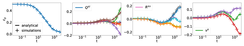
Figure 7: Agreement between simulations and ODEs when training a $K=3$ 2LNN on a Gaussian mixture in $D=800$ dimensions, with four Gaussian clusters with random covariance matrix $\Omega$ and random means (i.e. $\mu_{r}\!\sim\!\mathcal{N}(0,1)$) for sigmoidal activation function. We verify that even at finite ($D=800$) input dimension, the analytical prediction agree well with simulations. $\eta=0.1$, $g(x)=\mathrm{erf}\left(\nicefrac{{x}}{{\sqrt{2}}}\right)$, weights initialised with s.t.d. $\sigma_{0}=1$. Monte-Carlo integration performed with $10^{-4}$ samples.

Here, we verify the agreement of the ODEs derived above with simulation of 2LNN trained via online SGD.

To start, Fig. 7 displays the dynamics of a $K=3$ network trained on a Gaussian mixture with 4 Gaussian clusters having covariance matrix $\Omega=\nicefrac{{F^{T}F}}{{\sqrt{D}}}$ and means $\mu^{\alpha}$, where the elements of both the matrix $F\in\mathbb{R}^{D\times D}$ and the means are sampled i.i.d. from a standard Gaussian distribution. The agreement between analytical prediction, given by integration of the ODEs, and simulations is very good both in the dynamics of the test error, of the order parameters and of the second layer weights.

Note that the equations of motion describe the evolution of the densities $m$ and $q$ averaged over the input distribution. The agreement between this evolution and simulations justifies, at posteriori, the implicit assumption that the stochastic part of the SGD increment (7) can be neglected in the $D\to\infty$ limit. We can thus conjecture that in the $D\to\infty$ limit, the stochastic process defined by the SGD updates converges to a deterministic process parametrised by the continuous time variables $t\equiv\nicefrac{{N}}{{D}}$. We further add that the proof of this conjecture is not a straight-forward extension of the one of Goldt et al. (2019) for i.i.d. inputs since here, one must take into account the density of the covariance matrix.

The ODEs are valid for generic covariance matrix and means. Thus, they can be used to analyse the role of data structure in training 2LNNs. Although we leave a detailed analysis for future work, Fig. 8 gives an example of how this could be done in the case where a $K=3$ 2LNN is trained on a GM obtained from the FashionMnist dataset. The GM is obtained by computing the means $\bar{x}^{\alpha}$ and covariance matrix $\operatorname{\mathsf{Cov}}_{\alpha}(x,x)$ of each class in the dataset and assigning a label $+1$ or $-1$ to the different classes, as is commonly done in binary classification tasks. One could, for example, assign label $y=+1$ to the sneakers, boots, sandals, trousers and shorts categories and $y=-1$ to all others. Extending our analysis to $C$-class classification is straight forward and follows the analysis of Yoshida et al. (2019). The inputs are then sampled from a GM where the cluster’s mean are given by $\bar{x}^{\alpha}$ and the covariance matrix $\Omega$ is the mean covariance of all classes: $\Omega=\nicefrac{{1}}{{\text{n}_{\text{classes}}}}\sum\limits_{\alpha}\operatorname{\mathsf{Cov}}_{\alpha}(x,x)$. Note the similarity between this procedure and linear discriminant analysis commonly used in statistics. The agreement between simulations and analytical predictions is again very good, both at the level of the test error and of the order parameters.

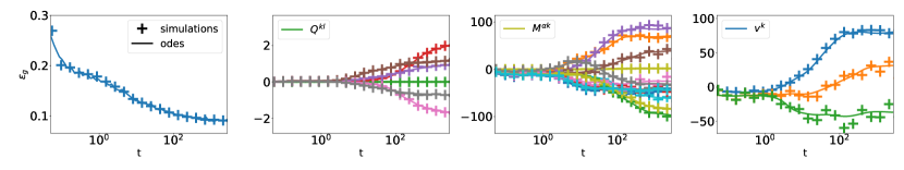
Figure 8: Agreement between simulations and ODEs when training a $K=3$ 2LNN with sigmoidal activation function on a Gaussian mixture obtained from the FashionMNIST dataset. The analytical dynamics obtained by integrating the ODEs agrees well with the given by simulations. Thus, the ODEs provide a tool to study the importance of datastructure in training 2LNN. We leave this study for future work. $D=784$, $\eta=0.1$, $g(x)=\mathrm{erf}\left(\nicefrac{{x}}{{\sqrt{2}}}\right)$, weights initialised with s.t.d. $\sigma_{0}=0.1$. Monte-Carlo integration performed with $10^{4}$ samples.

B.3 Simplified ansatz to solve the ODEs for the XOR-like mixture

Here, we detail the procedure, introduced in Sec. 2.3, used to find the long time $t\to\infty$ performance of 2LNN by making an ansatz on the form of the order parameters that solve the fix point equations. The motivation for doing so, as argued in of the main text, is that integrating the ODEs is numerically expensive as it requires evaluating various multidimensional integrals and the number of equations to integrate scales as $K^{2}$. In order to extract information about the asymptotic performances of the network, one can look for a fix point of the ODEs. However, the number of coupled equations to be solved, also scales quadraticaly with $K$ and is already $26$ for a $K=4$ student. The trick is to make an ansatz, with fewer degrees of freedom, on the order parameters that solve the equations. Used in this way, the ODEs have generated a wealth of analytical insights into the dynamics and the performance of 2LNN in the classical teacher-student setup (Biehl & Schwarze, 1995; Saad & Solla, 1995b, b; Biehl et al., 1996; Saad, 2009; Yoshida & Okada, 2019; Yoshida et al., 2019; Goldt et al., 2020b). In all these works though, an important simplification occured because the means of the local fields were all zero by construction. This simplification allowed the fixed points to be found analytically in some cases. Here, the means of the local fields evaluated over individual Gaussians in the mixture are not zero, so we have to resort to numerical means to find the fixed points of the ODEs.

Consider, for example, a 2LNN trained on the XOR-like mixture of Fig. 1. The Gaussian clusters have covariance $\Omega=\sigma^{2}\mathbb{I}$ and means chosen as in the left-hand-side diagram of Fig. 1, with the remaining $D-2$ components set to 0. This configuration leads to the constrain $w^{k}\cdot\mu^{\pm 0}=-w^{k}\cdot\mu^{\pm 1}$ that, in terms of overlap matrices, forces $M^{\alpha k}=-M^{\alpha+1k}$ thus halving the number of free parameters in $M$. It is also clear that the only components of the weight vectors which contribute to the error are those in the plane spanned by the means of the mixture. The additional $D-2$ components can be taken to $0$: i.e. $w^{k}_{r}=0$ for $r=2,..,D$. This condition allows to decompose the weight vectors as:

$$w_{s}^{k}=\sum_{r}\frac{w^{k}_{r}\mu_{r}^{+0}}{\sqrt{D}}\frac{\mu_{s}^{+0}}{\sqrt{D}}+\sum_{r}\frac{w^{k}_{r}\mu_{r}^{-0}}{\sqrt{D}}\frac{\mu_{s}^{-0}}{\sqrt{D}}$$ (B.29)

This decomposition, fully constrains the overlap matrix $Q^{kl}$ in terms of $M^{\alpha k}$:

$$\begin{split}Q^{kl}&=\sigma^{2}\sum_{s}\frac{w_{s}^{k}w_{s}^{l}}{D}\\ &=\sigma^{2}\left(\sum_{r}\frac{w^{k}\mu_{r}^{+0}}{D}\right)\left(\sum_{a}\frac{w^{l}_{a}\mu_{a}^{+0}}{D}\right)\frac{|\mu^{+0}|^{2}}{D}+\sigma^{2}\left(\sum_{r}\frac{w^{k}_{r}\mu_{r}^{-0}}{D}\right)\left(\sum_{a}\frac{w^{l}_{a}\mu_{a}^{-0}}{D}\right)\frac{|\mu^{-0}|^{2}}{D}\\ \Longrightarrow Q^{kl}&=\sigma^{2}\left(M^{+0k}M^{+0l}+M^{-0k}M^{-0l}\right),\end{split}$$ (B.30)

where we used that in the XOR-like mixture, $|\mu^{\alpha}|=\sqrt{D}$ and $\mu^{0+}\cdot\mu^{0-}=0$. From the symmetry between the positive and negative sign clusters of the mixture, in the fix point configuration, for every weight having norm $|w|$ and at an angle $\alpha$ with the mean of a positive cluster, there is a corresponding weight of the same norm, at an angle $\alpha$ with a negative mean. I.e. the angles of the weight vectors $w^{k}$ to the means $\mu^{\alpha}$, as well as the norms of the weights, are $2\times 2$ equal (one for the positive sign cluster and the other for the negative sign one). This constrains further half the number of free parameters in the overlap matrix $M$, which are down to $4K/(2\times 2)=K$. The second layer weights $v$ are fully constrained by requiring the output of the student to be $\pm 1$ when evaluated on the means. Putting everything together, one is left with $K$ equations to solve for the $\nicefrac{{K}}{{2}}$ angles and the $\nicefrac{{K}}{{2}}$ norms, or equivalently, for the $K$ free parameters in the overlap matrix $M$. The agreement between the solution found by solving this reduced set of equations and simulations is displayed both in Fig. 3, where we use it to predict the evolution of the test error with the $L2-$regularisation constant.

Appendix C Transforming a Gaussian mixture with random features

C.1 The distribution of random features is still a mixture

Given an input $x=(x_{i})\in\mathbb{R}^{D}$ sampled from the distribution (6), we consider the feature vector $z=(z_{i})\in\mathbb{R}^{N}$

$$z_{i}=\psi(u_{i}),\qquad u_{i}\equiv\sum_{r=1}^{D}\frac{1}{\sqrt{D}}F_{ir}x_{r}$$ (C.1)

where $F\in\mathbb{R}^{D\crossproduct P}$ is a random projection matrix and $\psi:\mathbb{R}\to\mathbb{R}$ is an element-wise non linearity. The distribution of $z$ can be computed as:

$$p_{z}(z) =\int_{\mathbb{R}^{D}}dxp_{x}(x)\delta\left(z-\psi\left(\frac{xF}{\sqrt{D}}\right)\right)$$

$$=\int_{\mathbb{R}^{D}}dx\sum_{y}q(y)q(x|y)\delta\left(z-\psi\left(\frac{xF}{\sqrt{D}}\right)\right)$$

$$\equiv\sum_{y}q(y)\sum_{\alpha\in\mathcal{S}\left(y\right)}\mathcal{P}_{\alpha}p_{z}^{\alpha}(z),$$ (C.2)

with

$$p_{z}^{\alpha}(z)=\int_{\mathbb{R}^{D}}dx\delta\left(z-\psi\left(\frac{xF}{\sqrt{D}}\right)\right)\mathcal{N}_{\alpha}\left(\frac{\mu^{\alpha}}{\sqrt{D}},\Omega^{\alpha}\right)$$ (C.3)

Crucially, the distribution of the features $z$ is still a mixture of distributions. We can thus restrict to studying the transformation of a Gaussian random variable

$$x_{r}=\frac{\mu_{r}}{\sqrt{D}}+\sigma w_{r}$$ (C.4)

where $w_{r}$ is a standard Gaussian. The scaling of $\mu_{r}$ and $\sigma$ is chosen according to which regime (low or high $\operatorname{\sf snr}$) one chooses to study. We aim at computing the distribution, in particular the two first moments, of the feature $z$ defined in Eq. (C.1). By construction, the random variables $u_{i}$ are Gaussian with first two moments:

$$\mathbb{E}\,u_{i}=\frac{1}{\sqrt{D}}\tilde{\mu}_{i},\qquad\tilde{\mu}_{i}\equiv\sum_{r}\frac{F_{ir}\mu_{r}}{\sqrt{D}}$$ (C.5)

$$\mathbb{E}\,u_{i}u_{j}=\frac{1}{D}\tilde{\mu}_{i}\tilde{\mu}_{j}+\sigma^{2}\sum_{r}\frac{F_{ir}F_{jr}}{D}$$ (C.6)

C.2 Low signal-to-noise ratio

Here we compute the statistics of the features, for general activation function, in the low signal to noise regime, for which $\nicefrac{{|\mu|}}{{\sqrt{D}}}\sim O(1)$ and $\sigma\sim O(1)$ so that the Gaussian clusters are a distance of order 1 away from the origin.

The mean of $z_{i}$ can be written as:

$$\mathbb{E}\,z_{i}=\mathbb{E}\,\psi(u_{i})=\mathbb{E}\,\psi\left(\frac{\tilde{\mu}_{i}}{\sqrt{D}}+\sigma\zeta\right),$$ (C.7)

where $\zeta\in\mathbb{R}$ is a standard Gaussian variable. In the scaling we work in, where $P$ and $D$ are send to infinity with their ratio fixed, and $\nicefrac{{|\mu|}}{{\sqrt{D}}}\sim O(1)$, $\tilde{\mu}_{i}/\sqrt{D}$ is of order $O(\nicefrac{{1}}{{\sqrt{D}}})$. Thus, the activation function $\psi$ can be expanded around $\sigma\zeta$:

$$\mathbb{E}\,z_{i}=\mathbb{E}\,\psi\left(\sigma\zeta\right)+\frac{\tilde{\mu}_{i}}{\sigma\sqrt{D}}\mathbb{E}\,\zeta\psi\left(\sigma\zeta\right)+O\left(\frac{1}{D}\right).$$ (C.8)

where we used integration by part to find $\sigma\mathbb{E}\,\partial\psi\left(\sigma\zeta\right)=\mathbb{E}\,\zeta\psi\left(\sigma\zeta\right)$.

For the covariance matrix, we separate the computation of the diagonal from the off-diagonal. Starting with the diagonal elements:

$$\begin{split}\mathbb{E}\,[z_{i}^{2}]=&\mathbb{E}\,\left[\left(\psi\left(\sigma\zeta\right)+\frac{\tilde{\mu}_{i}}{\sigma\sqrt{D}}\partial\psi\left(\sigma\zeta\right)\right)^{2}\right]\\ =&\mathbb{E}\,\left[\psi\left(\sigma\zeta\right)^{2}\right]+\frac{\tilde{\mu}_{i}}{\sigma\sqrt{D}}\mathbb{E}\,\zeta\psi^{2}\left(\sigma\zeta\right)+O\left(\frac{1}{D}\right)\end{split}$$ (C.9)

where, once gain, integration by parts was used to obtain $2\sigma\mathbb{E}\,\left[\psi\left(\sigma\zeta\right)\partial\psi\left(\sigma\zeta\right)\right]=\mathbb{E}\,\zeta\psi^{2}\left(\sigma\zeta\right)$.

In order to compute the off-diagonal elements, we note that different components of $u$ are weakly correlated since $\operatorname{Cov}(u_{i},u_{j})=\sigma^{2}\sum_{r}\nicefrac{{F_{ir}F_{jr}}}{{D}}\!\sim\!O(1/\sqrt{D})$. We can therefore apply formula Eq. (B.1) for weakly correlated variables:

$$\mathop{\mathbb{E}\,}_{(z_{i},z_{j})}z_{i}z_{j} =\mathop{\mathbb{E}\,}_{(u_{i},u_{j})}\psi(u_{i})\psi(u_{j})$$

$$=\mathop{\mathbb{E}\,}_{u_{i}}\psi(u_{i})\mathop{\mathbb{E}\,}_{u_{j}}\psi(u_{j})+\frac{1}{\sigma^{2}}\sum_{r}\frac{F_{ir}F_{jr}}{D}\mathop{\mathbb{E}\,}_{u_{i}}u_{i}\psi(u_{i})\mathop{\mathbb{E}\,}_{u_{j}}u_{j}\psi(u_{j})+O(\frac{1}{D})$$ (C.10)

where the averages are now over the one dimensional distributions of $u_{i}\!\sim\!\mathcal{N}\left(\frac{\tilde{\mu}_{i}}{\sqrt{D}},\sigma^{2}\right)$. We can now replace in the above $u_{i}=\frac{\tilde{\mu}_{i}}{\sqrt{D}}+\sigma\zeta$ and keep only leading order terms:

$$\begin{split}\operatorname{\mathsf{Cov}}(z_{i},z_{j})&=\sum_{r}\frac{F_{ir}F_{jr}}{\sigma^{2}D}\left(\psi(\sigma\zeta+\frac{\mu_{i}}{\sqrt{D}})(\sigma\zeta+\frac{\mu_{i}}{\sqrt{D}})\right)\left(\psi(\sigma\zeta+\frac{\mu_{j}}{\sqrt{D}})(\sigma\zeta+\frac{\mu_{j}}{\sqrt{D}})\right)\\ &=\sum_{r}\frac{F_{ir}F_{jr}}{\sigma^{2}D}\left(\psi(\sigma\zeta)\sigma\zeta+O(\frac{1}{\sqrt{D}})\right)\left(\psi(\sigma\zeta)\sigma\zeta+O(\frac{1}{\sqrt{D}})\right)\\ &=\mathbb{E}\,[\zeta\psi(\sigma\zeta)]^{2}\sum_{r}\frac{F_{ir}F_{jr}}{D}+O\left(\frac{1}{D}\right)\quad\text{, for }i\neq j.\end{split}$$ (C.11)

Thus yielding the final result:

$$\operatorname{\mathsf{Cov}}(z_{i},z_{j})=\mathbb{E}\,[\zeta\psi(\sigma\zeta)]^{2}\sum_{r}\frac{F_{ir}F_{jr}}{D}\quad\text{, for }i\neq j.$$ (C.12)

We define the constants $a$, $b$ and $c$ as in Eq. (18) and $d$ as:

$$a=\mathbb{E}\,\psi\left(\sigma\zeta\right),\quad b=\mathbb{E}\,\zeta\psi\left(\sigma\zeta\right),\quad c^{2}=\mathbb{E}\,\left[\psi\left(\sigma\zeta\right)^{2}\right],\quad d^{2}=\mathbb{E}\,\zeta\psi^{2}\left(\sigma\zeta\right)$$ (C.13)

These definitions together with Eq. (C.8), Eq. (C.9) and Eq. (C.12) lead to the statistics of Eq. (19) and Eq. (20):

$$\mathbb{E}\,z_{i} =a+\frac{\tilde{\mu}_{i}}{\sigma\sqrt{D}}b$$

$$\operatorname{\mathsf{Cov}}(z_{i},z_{j}) =\begin{cases}c^{2}-a^{2}+\underbrace{\frac{\tilde{\mu}_{i}}{\sigma\sqrt{D}}\left(d^{2}-2ab\right)}_{O(\frac{1}{\sqrt{D}})\text{: subleading if $c^{2}-a^{2}>0$}}+O(\frac{1}{D})\quad\text{, if }i=j\\ b^{2}\sum_{r}\frac{F_{ir}F_{jr}}{D}+O(\frac{1}{D})\quad\text{, if }i\neq j\end{cases}$$ (C.14)

The above shows that, the transformation of the means is only linear and in the low $\operatorname{\sf snr}$ regime, the XOR-like mixture of Fig. 1, is transformed into a XOR-like mixture in feature space which cannot be learned by linear regression. Note, that the performance of linear regression on the features is equivalent to its performance on inputs $\tilde{z}\in\mathbb{R}^{P}$ sampled from a Gaussian equivalent model defined as:

$$\tilde{z}_{i}=\mathbb{E}\,z_{i}+\sum_{j}\Omega^{1/2}_{ij}\zeta_{j},$$ (C.15)

where $\operatorname{\mathsf{Cov}}(z_{i},z_{j})\equiv\sum_{k}\Omega^{1/2}_{ik}\Omega^{1/2}_{jk}$ and $\zeta\in\mathbb{R}^{P}$ is a random vector with components sampled i.i.d. from a standard Gaussian distribution.

C.3 ReLU features

In the case of Relu activation function i.e. $\psi(x)=\max(0,x)$, the mean and the covariance of the features can be evaluated analytically for all $\operatorname{\sf snr}$ regimes. The distribution of the features within each cluster is given by a modified Gaussian: the probability mass of the Gaussian on the negative real axis is concentrated at the origin while the distribution on the positive axis is unchanged.

In particular, the integral to obtain the mean of $z$ can be computed analytically and is given by:

$$\mathbb{E}\,z_{i}=\mathbb{E}\,\operatorname{ReLU}(u_{i})=\sigma\left[\frac{\tilde{\rho}_{i}}{2}\left(1+\operatorname{erf}(\frac{\tilde{\rho}_{i}}{\sqrt{2}})\right)+\frac{1}{\sqrt{2\pi}}e^{-\tilde{\rho}_{i}^{2}/2}\right],$$ (C.16)

where we defined:

$$\tilde{\rho}_{i}\equiv\frac{\tilde{\mu}_{i}}{\sqrt{D}\sigma}=\frac{\sum_{r}F_{ir}\mu_{r}}{D\sigma}.$$

The covariance is once again computed by separating the diagonal terms from the off-diagonal ones. The integral to obtain the diagonal terms has an analytical expression found to be:

$$\operatorname{\mathsf{Cov}}(z_{i},z_{i})\!=\!\mathbb{E}\,[\operatorname{ReLU}(u_{i})^{2}]\!-\!\mathbb{E}\,[\operatorname{ReLU}(u_{i})]^{2}\!=\!\sigma^{2}\left[\frac{\tilde{\rho}_{i}}{\sqrt{2\pi}}e^{-\tilde{\rho}_{i}^{2}/2}+\frac{1}{2}(\tilde{\rho}_{i}^{2}+1)(1+\operatorname{erf}(\frac{\tilde{\rho}_{i}}{\sqrt{2}}))-(\mathbb{E}\,z_{i})^{2}\right]$$ (C.17)

For the off-diagonal components, we again use that the covariance of the different components of the $u_{i}$ is of order $\nicefrac{{1}}{{\sqrt{D}}}$ as $\operatorname{\mathsf{Cov}}(u_{i},u_{j})=\sigma^{2}\sum_{r}\nicefrac{{F_{ir}F_{jr}}}{{D}}$. Therefore, to evaluate $\mathbb{E}\,[\operatorname{ReLU}(u_{i})\operatorname{ReLU}(u_{j})]$, we can use the result Eq. (B.1) for weakly correlated variables with $\epsilon M_{12}=\sigma^{2}\sum_{r}\nicefrac{{F_{ir}F_{jr}}}{{D}}$. Then to leading order in $\frac{1}{D}$, one finds:

$$\begin{split}\operatorname{Cov}(z_{i},z_{j})&=\mathbb{E}\,[\operatorname{ReLU}(u_{i})\operatorname{ReLU}(u_{j})]-\mathbb{E}\,[\operatorname{ReLU}(u_{i})]\mathbb{E}\,[\operatorname{ReLU}(u_{j})]\\ &=\sum_{r}\frac{F_{ir}F_{jr}}{\sigma^{2}D}\mathbb{E}\,[u_{i}\operatorname{ReLU}(u_{i})]\mathbb{E}\,[u_{j}\operatorname{ReLU}(u_{j})]+O(\frac{1}{D})\end{split}$$ (C.18)

where the expectations above are over one dimensional distributions $u_{i}\sim\mathcal{N}\left(\sum_{r}\frac{F_{ir\mu_{r}}}{D},\sigma^{2}\right)$. The integrals have an analytical closed form expression, which yields the final result for the covariance:

$$\begin{split}\operatorname{Cov}(z_{i},z_{j})=\begin{cases}\sigma^{2}\left[\frac{\tilde{\rho}_{i}}{\sqrt{2\pi}}e^{-\tilde{\rho}_{i}^{2}/2}+\frac{1}{2}(\tilde{\rho}_{i}^{2}+1)(1+\operatorname{erf}(\frac{\tilde{\rho}_{i}}{\sqrt{2}}))-(\mathbb{E}\,z_{i})^{2}\right]\quad\text{if }i=j,\\ \frac{\sigma^{2}}{4}\frac{\sum_{r}F_{ir}F_{jr}}{D}\left(1+\operatorname{erf}(\frac{\tilde{\rho}_{i}}{\sqrt{2}})\right)\left(1+\operatorname{erf}(\frac{\tilde{\rho}_{j}}{\sqrt{2}})\right)+O(\frac{1}{D})\qquad\text{if }i\neq j\end{cases}\end{split}$$ (C.19)

C.4 Relation with the kernel

As discussed in Sec. 3 of the main text , the performances of kernel methods can be studied by using the convergence of RF to a kernel in the $\gamma\to\infty$ limit taken after the $D,P\to\infty$ limit (Rahimi & Recht, 2008):

$$K(x,y)\!=\!\frac{1}{P}\!\sum_{i=1}^{P}\mathop{\mathbb{E}\,}_{F}\!\left[\psi\left(\sum_{r=1}^{D}\frac{x_{r}F_{ir}}{\sqrt{D}}\right)\psi\left(\sum_{s=1}^{D}\frac{y_{s}F_{is}}{\sqrt{D}}\right)\right],$$

In the low $\operatorname{\sf snr}$ regime where $\nicefrac{{|\mu|}}{{\sqrt{D}}}\sim O(1)$, the action of the kernel is essentially linear. The three constants $a$, $b$ and $c$, defined in Eq. (18), can be expressed equivalently in terms of the activation function $\psi$ or of the kernel. Consider $\omega_{1}$, $\omega_{2}\in\mathbb{R}$, two i.i.d. standard Gaussian random variables, and denote by angle brackets $\langle\cdot\rangle$ the expectation over $w_{1},w_{2}$. Then, by the definition $K(x,y)$ one has:

$$\langle K(\sigma\omega_{1},\sigma\omega_{1})\rangle=\frac{1}{P}\sum_{i=1}^{P}\langle\psi(u_{i})^{2}\rangle=c^{2}$$ (C.20)

where $u\in\mathbb{R}^{P}$ is the random vector whose moments are defined in Eq. (C.5) and we used the element wise convergence of $\nicefrac{{\psi(\sum_{r}F_{ir}x_{r})\psi(\sum_{r}F_{is}y_{s})}}{{P}}$ to its expected value (Rahimi & Recht, 2008). Similarly, one has:

$$\langle K(\sigma\omega_{1},\sigma\omega_{2})\rangle=\frac{1}{P}\sum_{i=1}^{P}\langle\psi(u_{i})\rangle^{2}=a^{2}$$ (C.21)

Finally, for $b$ one has to perform a linear expansion of the kernel around the noise variable $\sigma\omega_{\begin{subarray}{c}1\\ 2\end{subarray}}$:

$$\langle K(\sigma\omega_{1}+\frac{\mu}{\sqrt{D}},\sigma\omega_{2}+\frac{\mu}{\sqrt{D}})\rangle= \frac{1}{P}\sum_{i=1}^{P}\langle\mathop{\mathbb{E}\,}_{F}\left[\psi(u_{i1}+\sum_{r}\frac{\mu_{r}F_{ir}}{D})\rangle\langle\psi(u_{i2}+\sum_{r}\frac{\mu_{r}F_{ir}}{D})\right]\rangle$$

$$= \frac{1}{P}\sum_{i=1}^{P}\langle\psi(u_{i})\rangle^{2}+\sum_{rs}\frac{\mu_{r}\mu_{s}}{D^{2}}\sum_{i=1}^{P}\mathop{\mathbb{E}\,}_{F}\frac{F_{ir}F_{is}}{P}\langle\psi^{\prime}(u_{i})\rangle^{2}$$

$$= a^{2}+\frac{1}{D\sigma^{2}}b^{2},$$

$$\Longrightarrow b^{2}= D\sigma^{2}\left(-a^{2}+\langle K(\sigma\omega_{1}+\frac{\mu}{\sqrt{D}},\sigma\omega_{2}+\frac{\mu}{\sqrt{D}})\rangle\right)$$ (C.22)

These expressions allow to express the statistical properties of the features $z$, and to asses the performance of RF and kernel methods, directly in terms of the kernel without requiring the explicit form of the activation function.

For completeness, we give the analytical expression of the kernel corresponding to ReLU random features, i.e. $\psi(x)=\max(0,x)$:

$$K_{\text{ReLU}}(x,y)=\frac{|x||y|}{8\pi D}\left\{2|\sin(\theta)|+\cos(\theta)\left(\pi+2\operatorname{Arctan}\left(\frac{\cos(\theta)}{|\sin(\theta)|}\right)\right)\right\},$$ (C.23)

where we defined the angle $\theta$ between the two vectors $x,y\in\mathbb{R}^{D}$ such that $|x|,|y|>0$:

$$\theta=\frac{x\cdot y}{|x||y|}$$ (C.24)

From Eq. (C.23), one sees that in case of ReLU activation function, the kernel is an angular kernel, i.e. it depends on the angle between $x$ and $y$.

Appendix D Final test error of random features

This section details the computations leading to Eq. (14) and Eq. (16) allowing to obtain the asymptotic performances of RF trained via online SGD on a mixture of Gaussian distribution.

Applying random features on $x\in\mathbb{R}^{D}$ sampled from the distribution (6) is equivalent to performing linear regression on the features $z\in\mathbb{R}^{P}$ with covariance $\Omega^{z}$ and mean $\mu_{z}$. In the following, for clarity, we assume the features are centred, so that $\mu_{z}=0$, extending the computation to non centred features is straight-forward. The means of the individual clusters are however non zero. The output of the network at a step $t$ in training is given by $\phi(w)_{t}=\sum_{i=1}^{P}\nicefrac{{w_{i}z_{ti}}}{{\sqrt{P}}}$. We train the network in the online limit by minimising the squared loss between the output of the network and the label $y_{t}$. The $\operatorname{\sf pmse}$ is given by:

$$\operatorname{\sf pmse}(w)=\frac{1}{2}\mathbb{E}\,\left(y-\sum_{i=1}^{P}\frac{w_{i}z_{i}}{\sqrt{P}}\right)^{2}=\frac{1}{2}+\sum_{i,j=1}^{P}\frac{w_{i}w_{j}}{2P}\Omega^{z}_{ij}-\sum_{i=1}^{P}\frac{w_{i}}{\sqrt{P}}\Phi_{i},$$ (D.1)

where we introduced the input-label covariance $\Phi_{i}\equiv\mathbb{E}\,[z_{i}y]$.

The expectation of the SGD update over the distribution of $z$ is thus:

$$\mathbb{E}\,\operatorname{d}\!w_{i} =-\frac{\eta}{\sqrt{P}}\mathbb{E}\,z_{i}\left(\sum_{j=1}^{P}\frac{w_{j}z_{j}}{\sqrt{P}}-y\right)=\frac{\eta}{\sqrt{P}}(\Phi_{i}-\sum_{j=1}^{P}\frac{w_{j}}{\sqrt{P}}\Omega^{z}_{ij})$$ (D.2)

Importantly, both the $\operatorname{\sf pmse}$ and the average update only depend on the distribution of the features through the covariance matrix of the features $\Omega^{z}$ and the input label covariance $\Psi$.

To make progress, consider the eigen-decomposition of the covariance matrix $\Omega^{z}$:

$$\Omega_{ij}^{z}=\frac{1}{P}\sum_{\tau}\rho_{\tau}\Gamma_{\tau i}\Gamma_{\tau j},$$ (D.3)

where $\rho_{\tau}$ are the eigenvalues and $\Gamma_{\tau}$ their corresponding eigenvectors.

Define the rotation of $W$ and $\Phi$ into this eigenbasis:

$$\tilde{w}_{\tau}\equiv\frac{1}{\sqrt{P}}\sum_{i=1}^{P}\Gamma_{i\tau}w_{i}\quad\tilde{\Phi}_{\tau}\equiv\frac{1}{\sqrt{P}}\sum_{i=1}^{P}\Gamma_{i\tau}\Phi_{i}$$ (D.4)

In this basis, the SGD update for the different components of $\tilde{W}$ decouple. One finds a recursive equation in which each mode evolves independently from the others:

$$\mathbb{E}\,\operatorname{d}\!\tilde{w}_{\tau}=\frac{\eta}{\sqrt{P}}(\tilde{\Phi}_{\tau}-\frac{1}{\sqrt{P}}\sum_{\tau=1}^{P}\rho_{\tau}\tilde{w}_{\tau})$$ (D.5)

Thus, the fix point $\tilde{\hat{W}}$ such that $\mathbb{E}\,\operatorname{d}\!\tilde{\hat{w}}_{\tau}=0$, can be found explicitly:

$$\rho_{\tau}\tilde{\hat{w}}_{\tau}=\sqrt{P}\tilde{\Phi}_{\tau}.$$

Rotating back in the original basis one finds the asymptotic solution for $W$ as:

$$\hat{w}_{i}=\sum_{\tau;\rho_{\tau}>0}\frac{1}{\rho_{\tau}}\Gamma_{i\tau}\tilde{\Phi}_{\tau}.$$ (D.6)

The asymptotic test error is thus given by:

$$\operatorname{\sf pmse}_{t\to\infty}=\frac{1}{2}\left(1-\sum_{\tau}\frac{\tilde{\Phi}_{\tau}^{2}}{\rho_{\tau}}\right)$$ (D.7)

Asymptotic classification error

From the solution of Eq. (D.6) for the asymptotic solution found by linear regression, one can obtain the asymptotic classification error performed by random features as:

$$\epsilon_{ct\to\infty}=\mathbb{E}\,\Theta(-y\lambda)=\sum_{\alpha}\mathcal{P}_{\alpha}\mathop{\mathbb{E}\,}_{\alpha}\Theta(-y\lambda),$$ (D.8)

where $\Theta:\mathbb{R}\to\mathbb{R}$ is the Heaviside step function and we defined $\lambda\equiv\sum_{i=1}^{P}\nicefrac{{\hat{w}_{i}z_{i}}}{{\sqrt{P}}}$. Introducing the local field $\lambda$ allows to transform the high dimensional integral over the features $z$ into a low-dimensional (in this case one dimensional) expectation over the local field. The Gaussian equivalency theorem of Goldt et al. (2020a) shows that even though the $z$ are not Gaussian, to leading order in $1/P$, the average Eq. (16), only depends on the first two moments $\lambda$, defined as:

$$M_{\alpha}=\mathop{\mathbb{E}\,}_{\alpha}[\lambda]=\sum_{i=1}^{P}\frac{\hat{w}_{i}\mathop{\mathbb{E}\,}_{\alpha}[z_{i}]}{\sqrt{P}}\quad Q_{\alpha}=\mathop{\operatorname{\mathsf{Cov}}}_{\alpha}[\lambda,\lambda]=\sum_{i=1}^{P}\frac{\hat{w}_{i}\hat{w}_{j}}{P}\mathop{\operatorname{\mathsf{Cov}}}_{\alpha}(z,z)$$ (D.9)

These moments can be computed analytically from the statistics of the features computed in Sec. C and from the optimal weights $W$ obtained in Eq. (D.6). The classification error, Eq. (D.8), can thus be evaluated by means of a one dimensional integral over the distribution of $\lambda$.

$$\epsilon_{ct\to\infty} =\sum_{\alpha}\mathcal{P}_{\alpha}\int\frac{d\lambda}{\sqrt{2\pi Q_{\alpha}}}\Theta(-y_{\alpha}\lambda)e^{-\frac{1}{2Q_{\alpha}}(\lambda-M_{\alpha})^{2}}$$ (D.10)

$$=\frac{1}{2}\left(1-\sum_{\alpha}\mathcal{P}_{\alpha}y_{\alpha}\mathrm{erf}\left(\frac{M_{\alpha}}{\sqrt{2Q_{\alpha}}}\right)\right)$$ (D.11)

Appendix E The three-cluster model

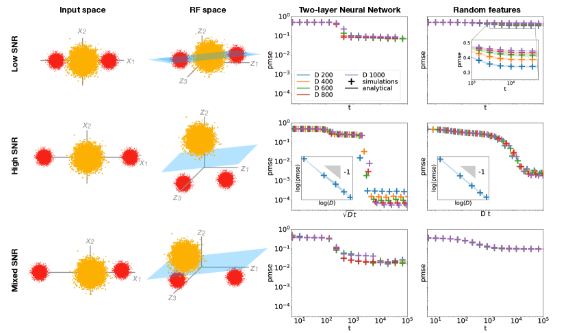
Figure 10: We compare the performance of 2LNN with $K=10$ hidden units and ReLU activation function (third column) to the ones of random features (fourth column) on the three cluster problem with different signal-to-noise ratios. The right sketches the input space distribution and the second column the transformed distribution in feature space. 2LNN can considerably outperform RF in all three regimes. In the low $\operatorname{\sf snr}$ regime (top), the action of the random features is essentially linear inducing their performance to be as bad as random guessing in the $D\to\infty$ limit. In the high $\operatorname{\sf snr}$ regime (middle), instead, both networks manage to learn the task. In the mixed $\operatorname{\sf snr}$ regime (bottom), the distance between opposite sign clusters remains of orther one in feature space inducing the RF performances to be unchanged with $D$. We plot the test error as a function of time. Parameters: $D=1000$, $\eta=0.1$, $\sigma^{2}=0.05$, $P=2D$ for random features, $K=10$ for 2LNN.

Similar to the analysis of the XOR-like mixture of Fig. 6, we analyse a data model with three clusters that was the subject of several recent works (Deng et al., 2019; Mai & Liao, 2019; Lelarge & Miolane, 2019; Mignacco et al., 2020a, b). The Gaussian mixture in input space can be seen in the first column of Fig. 10. The means of both positive clusters are set to $0$ while the means of the negative sign clusters have first component $\pm\mu_{0}$ and all other $D-1$ components $0$. The mixture after random feature transformation is displayed in the second column and the third and fourth column show the performance of a 2LNN, respectively, a random feature network, trained via online SGD, on this problem. Here again, we build on the observation that overparametrisation does not impact performances and train a $K=10$ 2LNN in order to increase the number of runs that converged. The three rows, are as before, three different $\operatorname{\sf snr}$ regimes, they are in order the low, high and mixed $\operatorname{\sf snr}$ regime.

The phenomenology observed in the XOR-like mixture carries through here. In the low $\operatorname{\sf snr}$ regime, $\mu_{0}=\sqrt{D}$ (top row), the 2LNN can learn the problem and its performance remains constant with increasing input dimension. On the other hand, in this regime, the transformation performed by the random features is only linear in the large $D$ limit. Consequently, the RF performances degrade with increasing $D$ and are as bad as random chance in the limit of infinite input dimension. In the high $\operatorname{\sf snr}$ regime instead (second row), where $\mu_{0}=D$, the mixtures becomes well separated in feature space allowing RF to perform well. Both the performance of 2LNN and RF improve as the clusters in the mixture become more separated. The mixed $\operatorname{\sf snr}$ regime (bottom row) is obtained by setting one of the negative sign clusters a distance $\sqrt{D}$ from the origin while maintaining the other one at a distance $1$. Here, the random feature perform a non trivial transformation of the far away cluster while its action on the nearby cluster is linear. Hence, in feature space, one of the negative clusters remains close to the positive clusters while the other is well separated. The RF thus achieve a test error which is better than random but still worse that that of the 2LNN. Its error is constant with increasing $D$ since it is dominated by the “spill-over” of the negative cluster into the positive cluster at the origin.

Lastly, let us comment that in all our work, we did not add a bias to the model. Adding a bias, does not change the conclusion that small 2LNN considerably outperform RF. In fact, the learning curves are only slightly modified. This is due to to our minimisation of the $\operatorname{\sf pmse}$ when training the network, which, unlike classification loss that only cares about the sign of the estimate, penalises large differences between label $y=\pm 1$ and the output. For simplicity, we thus chose to remove the bias in our analysis, although including it is a straight forward operation.

References

- Allen-Zhu et al. (2018) Allen-Zhu, Z., Li, Y., and Song, Z. A convergence theory for deep learning via over-parameterization. 2018.
- Allen-Zhu et al. (2019) Allen-Zhu, Z., Li, Y., and Song, Z. A convergence theory for deep learning via over-parameterization. In International Conference on Machine Learning, pp. 242–252. PMLR, 2019.
- Arora et al. (2018) Arora, S., Cohen, N., and Hazan, E. On the optimization of deep networks: Implicit acceleration by overparameterization. In International Conference on Machine Learning, pp. 244–253. PMLR, 2018.
- Arora et al. (2019) Arora, S., Du, S., Hu, W., Li, Z., Salakhutdinov, R., and Wang, R. On exact computation with an infinitely wide neural net. In Advances in Neural Information Processing Systems, pp. 8141–8150, 2019.
- Arous et al. (2020) Arous, G. B., Gheissari, R., and Jagannath, A. A classification for the performance of online sgd for high-dimensional inference. arXiv:2003.10409, 2020.
- Bach (2017) Bach, F. Breaking the curse of dimensionality with convex neural networks. The Journal of Machine Learning Research, 18(1):629–681, 2017.
- Barron (1993) Barron, A. R. Universal approximation bounds for superpositions of a sigmoidal function. IEEE Transactions on Information theory, 39(3):930–945, 1993.
- Biehl & Schwarze (1995) Biehl, M. and Schwarze, H. Learning by on-line gradient descent. J. Phys. A. Math. Gen., 28(3):643–656, 1995.
- Biehl et al. (1996) Biehl, M., Riegler, P., and Wöhler, C. Transient dynamics of on-line learning in two-layered neural networks. Journal of Physics A: Mathematical and General, 29(16), 1996.
- Cao & Gu (2019) Cao, Y. and Gu, Q. Generalization bounds of stochastic gradient descent for wide and deep neural networks. In Advances in Neural Information Processing Systems, pp. 10836–10846, 2019.
- Caponnetto & De Vito (2007) Caponnetto, A. and De Vito, E. Optimal rates for the regularized least-squares algorithm. Foundations of Computational Mathematics, 7(3):331–368, 2007.
- Chizat & Bach (2018) Chizat, L. and Bach, F. On the global convergence of gradient descent for over-parameterized models using optimal transport. In Advances in Neural Information Processing Systems 31, pp. 3040–3050, 2018.
- Chizat & Bach (2020) Chizat, L. and Bach, F. Implicit bias of gradient descent for wide two-layer neural networks trained with the logistic loss. In Conference on Learning Theory, pp. 1305–1338. PMLR, 2020.
- Chizat et al. (2019) Chizat, L., Oyallon, E., and Bach, F. On lazy training in differentiable programming. In Advances in Neural Information Processing Systems, pp. 2937–2947, 2019.
- Cohen et al. (2020) Cohen, U., Chung, S., Lee, D., and Sompolinsky, H. Separability and geometry of object manifolds in deep neural networks. Nature communications, 11(1):1–13, 2020.
- Couillet (2019) Couillet, R. High dimensional robust classification: A random matrix analysis. In 2019 IEEE 8th International Workshop on Computational Advances in Multi-Sensor Adaptive Processing (CAMSAP), pp. 420–424, 2019.
- Daniely & Malach (2020) Daniely, A. and Malach, E. Learning parities with neural networks. In Advances in Neural Information Processing Systems, volume 33, 2020.
- Deng et al. (2019) Deng, Z., Kammoun, A., and Thrampoulidis, C. A model of double descent for high-dimensional binary linear classification. arXiv:1911.05822, 2019.
- Du et al. (2019) Du, S., Zhai, X., Poczos, B., and Singh, A. Gradient descent provably optimizes over-parameterized neural networks. In International Conference on Learning Representations, 2019.
- El Karoui (2010) El Karoui, N. The spectrum of kernel random matrices. Ann. Statist., 38(1):1–50, 02 2010.
- Gardner & Derrida (1989) Gardner, E. and Derrida, B. Three unfinished works on the optimal storage capacity of networks. Journal of Physics A: Mathematical and General, 22(12):1983–1994, 1989.
- Garriga-Alonso et al. (2019) Garriga-Alonso, A., Rasmussen, C., and Aitchison, L. Deep convolutional networks as shallow gaussian processes. In International Conference on Learning Representations, 2019.
- Geiger et al. (2020) Geiger, M., Spigler, S., Jacot, A., and Wyart, M. Disentangling feature and lazy training in deep neural networks. Journal of Statistical Mechanics: Theory and Experiment, 2020(11):113301, 2020.
- Ghorbani et al. (2019) Ghorbani, B., Mei, S., Misiakiewicz, T., and Montanari, A. Limitations of lazy training of two-layers neural network. In Advances in Neural Information Processing Systems, volume 32, pp. 9111–9121, 2019.
- Ghorbani et al. (2020) Ghorbani, B., Mei, S., Misiakiewicz, T., and Montanari, A. When do neural networks outperform kernel methods? In Advances in Neural Information Processing Systems, volume 33, 2020.
- Goldt et al. (2019) Goldt, S., Advani, M., Saxe, A., Krzakala, F., and Zdeborová, L. Dynamics of stochastic gradient descent for two-layer neural networks in the teacher-student setup. In Advances in Neural Information Processing Systems 32, 2019.
- Goldt et al. (2020a) Goldt, S., Loureiro, B., Reeves, G., Mézard, M., Krzakala, F., and Zdeborová, L. The gaussian equivalence of generative models for learning with two-layer neural networks. arXiv:2006.14709, 2020a.
- Goldt et al. (2020b) Goldt, S., Mézard, M., Krzakala, F., and Zdeborová, L. Modeling the influence of data structure on learning in neural networks: The hidden manifold model. Phys. Rev. X, 10(4):041044, 2020b.
- Jacot et al. (2018) Jacot, A., Gabriel, F., and Hongler, C. Neural tangent kernel: Convergence and generalization in neural networks. In Advances in Neural Information Processing Systems 32, pp. 8571–8580, 2018.
- Kini & Thrampoulidis (2020) Kini, G. R. and Thrampoulidis, C. Analytic study of double descent in binary classification: The impact of loss. In 2020 IEEE International Symposium on Information Theory (ISIT), pp. 2527–2532. IEEE, 2020.
- Lee et al. (2018) Lee, J., Sohl-Dickstein, J., Pennington, J., Novak, R., Schoenholz, S., and Bahri, Y. Deep neural networks as gaussian processes. In International Conference on Learning Representations, 2018.
- Lelarge & Miolane (2019) Lelarge, M. and Miolane, L. Asymptotic bayes risk for gaussian mixture in a semi-supervised setting. In 2019 IEEE 8th International Workshop on Computational Advances in Multi-Sensor Adaptive Processing (CAMSAP), pp. 639–643. IEEE, 2019.
- Li & Liang (2018) Li, Y. and Liang, Y. Learning Overparameterized Neural Networks via Stochastic Gradient Descent on Structured Data. In Advances in Neural Information Processing Systems 31, 2018.
- Li et al. (2020) Li, Y., Ma, T., and Zhang, H. R. Learning over-parametrized two-layer neural networks beyond ntk. In Abernethy, J. and Agarwal, S. (eds.), Proceedings of Thirty Third Conference on Learning Theory, volume 125 of Proceedings of Machine Learning Research, pp. 2613–2682. PMLR, 2020.
- Li et al. (2019) Li, Z., Wang, R., Yu, D., Du, S. S., Hu, W., Salakhutdinov, R., and Arora, S. Enhanced convolutional neural tangent kernels. arXiv:1911.00809, 2019.
- Liao & Couillet (2018) Liao, Z. and Couillet, R. On the spectrum of random features maps of high dimensional data. In International Conference on Machine Learning, pp. 3063–3071. PMLR, 2018.
- Liao & Couillet (2019) Liao, Z. and Couillet, R. On inner-product kernels of high dimensional data. In 2019 IEEE 8th International Workshop on Computational Advances in Multi-Sensor Adaptive Processing (CAMSAP), pp. 579–583, 2019.
- Livni et al. (2014) Livni, R., Shalev-Shwartz, S., and Shamir, O. On the computational efficiency of training neural networks. In Advances in Neural Information Processing Systems, volume 27, pp. 855–863, 2014.
- Louart et al. (2018) Louart, C., Liao, Z., and Couillet, R. A random matrix approach to neural networks. The Annals of Applied Probability, 28(2):1190–1248, 2018.
- Mai & Liao (2019) Mai, X. and Liao, Z. High dimensional classification via empirical risk minimization: Improvements and optimality. arXiv preprint arXiv:1905.13742, 2019.
- Matthews et al. (2018) Matthews, A. G. d. G., Hron, J., Rowland, M., Turner, R., and Ghahramani, Z. Gaussian process behaviour in wide deep neural networks. In International Conference on Learning Representations, 2018.
- Mei & Montanari (2019) Mei, S. and Montanari, A. The generalization error of random features regression: Precise asymptotics and double descent curve. arXiv:1908.05355, 2019.
- Mei et al. (2018) Mei, S., Montanari, A., and Nguyen, P. A mean field view of the landscape of two-layer neural networks. Proceedings of the National Academy of Sciences, 115(33):E7665–E7671, 2018.
- Mei et al. (2021) Mei, S., Misiakiewicz, T., and Montanari, A. Generalization error of random features and kernel methods: hypercontractivity and kernel matrix concentration. arXiv preprint arXiv:2101.10588, 2021.
- Mignacco et al. (2020a) Mignacco, F., Krzakala, F., Lu, Y. M., and Zdeborová, L. The role of regularization in classification of high-dimensional noisy gaussian mixture. In 37th International Conference on Machine Learning, 2020a.
- Mignacco et al. (2020b) Mignacco, F., Krzakala, F., Urbani, P., and Zdeborová, L. Dynamical mean-field theory for stochastic gradient descent in gaussian mixture classification. In Advances in Neural Information Processing Systems (NeurIPS), 2020b.
- Paccolat et al. (2021) Paccolat, J., Petrini, L., Geiger, M., Tyloo, K., and Wyart, M. Geometric compression of invariant manifolds in neural networks. Journal of Statistical Mechanics: Theory and Experiment, 2021(4):044001, 2021. doi: 10.1088/1742-5468/abf1f3. URL https://doi.org/10.1088/1742-5468/abf1f3.
- Pennington & Worah (2017) Pennington, J. and Worah, P. Nonlinear random matrix theory for deep learning. In Advances in Neural Information Processing Systems, pp. 2637–2646, 2017.
- Rahimi & Recht (2008) Rahimi, A. and Recht, B. Random features for large-scale kernel machines. In Advances in neural information processing systems, pp. 1177–1184, 2008.
- Rahimi & Recht (2009) Rahimi, A. and Recht, B. Weighted sums of random kitchen sinks: Replacing minimization with randomization in learning. In Advances in neural information processing systems, pp. 1313–1320, 2009.
- Riegler & Biehl (1995) Riegler, P. and Biehl, M. On-line backpropagation in two-layered neural networks. Journal of Physics A: Mathematical and General, 28(20), 1995.
- Rotskoff & Vanden-Eijnden (2018) Rotskoff, G. and Vanden-Eijnden, E. Parameters as interacting particles: long time convergence and asymptotic error scaling of neural networks. In Advances in Neural Information Processing Systems 31, pp. 7146–7155, 2018.
- Saad (2009) Saad, D. On-line learning in neural networks, volume 17. Cambridge University Press, 2009.
- Saad & Solla (1995a) Saad, D. and Solla, S. Exact Solution for On-Line Learning in Multilayer Neural Networks. Phys. Rev. Lett., 74(21):4337–4340, 1995a.
- Saad & Solla (1995b) Saad, D. and Solla, S. On-line learning in soft committee machines. Phys. Rev. E, 52(4):4225–4243, 1995b.
- Saad & Solla (1997) Saad, D. and Solla, S. Learning with Noise and Regularizers Multilayer Neural Networks. In Advances in Neural Information Processing Systems 9, pp. 260–266, 1997.
- Safran & Shamir (2018) Safran, I. and Shamir, O. Spurious local minima are common in two-layer relu neural networks. In International Conference on Machine Learning, pp. 4433–4441. PMLR, 2018.
- Scholkopf & Smola (2018) Scholkopf, B. and Smola, A. Learning with kernels: support vector machines, regularization, optimization, and beyond. Adaptive Computation and Machine Learning series, 2018.
- Shankar et al. (2020) Shankar, V., Fang, A., Guo, W., Fridovich-Keil, S., Ragan-Kelley, J., Schmidt, L., and Recht, B. Neural kernels without tangents. In III, H. D. and Singh, A. (eds.), Proceedings of the 37th International Conference on Machine Learning, volume 119 of Proceedings of Machine Learning Research, pp. 8614–8623. PMLR, 2020.
- Sirignano & Spiliopoulos (2019) Sirignano, J. and Spiliopoulos, K. Mean field analysis of neural networks: A central limit theorem. Stochastic Processes and their Applications, 2019.
- Steinwart et al. (2009) Steinwart, I., Hush, D. R., Scovel, C., et al. Optimal rates for regularized least squares regression. In COLT, pp. 79–93, 2009.
- Suzuki & Akiyama (2020) Suzuki, T. and Akiyama, S. Benefit of deep learning with non-convex noisy gradient descent: Provable excess risk bound and superiority to kernel methods. arXiv preprint arXiv:2012.03224, 2020.
- Wang et al. (2019) Wang, C., Hu, H., and Lu, Y. A solvable high-dimensional model of gan. In Advances in Neural Information Processing Systems, pp. 13759–13768, 2019.
- Wei et al. (2019) Wei, C., Lee, J. D., Liu, Q., and Ma, T. Regularization matters: Generalization and optimization of neural nets v.s. their induced kernel. In Wallach, H., Larochelle, H., Beygelzimer, A., d'Alché-Buc, F., Fox, E., and Garnett, R. (eds.), Advances in Neural Information Processing Systems, volume 32. Curran Associates, Inc., 2019.
- Yehudai & Shamir (2019) Yehudai, G. and Shamir, O. On the power and limitations of random features for understanding neural networks. In Advances in Neural Information Processing Systems, volume 32, pp. 6598–6608, 2019.
- Yoshida & Okada (2019) Yoshida, Y. and Okada, M. Data-dependence of plateau phenomenon in learning with neural network — statistical mechanical analysis. In Advances in Neural Information Processing Systems 32, pp. 1720–1728, 2019.
- Yoshida et al. (2019) Yoshida, Y., Karakida, R., Okada, M., and Amari, S.-I. Statistical mechanical analysis of learning dynamics of two-layer perceptron with multiple output units. Journal of Physics A: Mathematical and Theoretical, 52(18):184002, 2019.