Causal Mediation Analysis with Hidden Confounders

Abstract.

An important problem in causal inference is to break down the total effect of a treatment on an outcome into different causal pathways and to quantify the causal effect in each pathway. For instance, in causal fairness, the total effect of being a male employee (i.e., treatment) constitutes its direct effect on annual income (i.e., outcome) and the indirect effect via the employee’s occupation (i.e., mediator). Causal mediation analysis (CMA) is a formal statistical framework commonly used to reveal such underlying causal mechanisms. One major challenge of CMA in observational studies is handling confounders, variables that cause spurious causal relationships among treatment, mediator, and outcome. Conventional methods assume sequential ignorability that implies all confounders can be measured, which is often unverifiable in practice. This work aims to circumvent the stringent sequential ignorability assumptions and consider hidden confounders. Drawing upon proxy strategies and recent advances in deep learning, we propose to simultaneously uncover the latent variables that characterize hidden confounders and estimate the causal effects. Empirical evaluations using both synthetic and semi-synthetic datasets validate the effectiveness of the proposed method. We further show the potentials of our approach for causal fairness analysis.

1. Introduction

Consider the following two real-world problems.

Example 1. An E-commerce platform (e.g., Amazon) wants to help sellers promote products by introducing a new feature in the recommendation module in addition to users’ organic search. However, with the two modules together contributing to the conversion rate, the improved performance of one module may render the effects of optimizing another module insignificant and sometimes even negative (Yin and Hong, 2019). For instance, the new recommendation feature successfully suggests products that fulfill users’ needs meanwhile notably curtails the user engagement in organic search.

Example 2. Researchers in fair machine learning want to examine if female employees are systematically discriminated in various companies. They collect data from US census that record whether a person earns more than $50,000/year, her age, gender, occupation, and other demographic information. A causal fairness analysis is conducted to estimate the effect of gender on the income: a nonzero effect might indicate discrimination. They further find out that the discrimination consists of the direct discrimination against female and the indirect discrimination against female through occupation.

Underpinning the previous phenomena is a causal mediation analysis (CMA) where the total effect of a treatment (e.g., the new feature or gender) on the outcome (e.g., conversion rate or income) constitutes a direct causal effect, e.g., gender $\rightarrow$ income, and an indirect causal effect through the intermediate variable – mediator, e.g., gender $\rightarrow$ occupation $\rightarrow$ income. CMA is a formal statistical framework aiming to quantify the direct effect and the indirect effect (causal mediation effect) of the treatment on the outcome. Despite its transparency and capability of fine-grained causal analysis, CMA confronts the conventional challenge when applied to observational studies: hidden confounders (HC), a set of hidden variables ${\bf Z}$ that affects causal relationships among the treatment $T$, mediator, ${\bf M}$ and outcome $Y$ (Imai et al., 2010), as shown in Fig. 1.

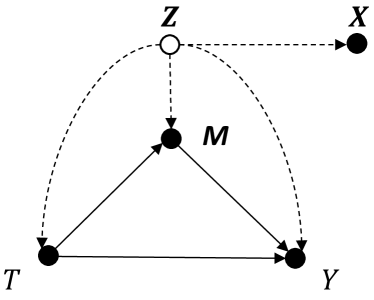
Figure 1. The causal diagram $G$ of CMA with proxy variables. ${\bf X}$ are the noisy proxies used to approximate HC (${\bf Z}$). Solid dots and edges represent observed variables and causal relationships.

Compared to standard causal inference, controlling for HC in CMA is even more challenging as confounders can lie on the causal pathways between any pair of variables among $T,{\bf M},Y$. For example, in Fig. 1, ${\bf Z}$ can lie on the path $T\rightarrow{\bf M}$ or ${\bf M}\rightarrow Y$ or both. Therefore, research in CMA often has recourse to the sequential ignorability assumption (Imai et al., 2010) which states that all confounders can be measured. This is clearly unverifiable in most observational studies, e.g., a user’s preference in Example 1 or a person’s sexual orientation in Example 2. Even gold-standard randomized experiments (Rubin, 2005) cannot provide us valid direct and indirect effect estimations in CMA (Keele, 2015) since we cannot randomize the mediator.

In this paper, we seek to circumvent the sequential ignorability assumption by considering HC. Prior causal inference research (Griliches and Hausman, 1986; Pearl, 2012) estimates total effect by imposing strong constraints on HC such as being categorical. Nevertheless, we cannot know the exact nature of HC (e.g., categorical or continuous), especially when HC can come from multiple sources induced by the mediator. To address this, we have recourse to the observed proxy variables ${\bf X}$ (Angrist and Pischke, 2008) under the assumption that proxies and HC are inherently correlated. For instance, we might approximate user preferences by measuring proxies such as her job type and zip code. The challenge in CMA with HC is that we need to perform three inferential tasks simultaneously: approximating HC and estimating direct and indirect effects. Following the recent success of deep learning in causal inference (e.g., (Shalit et al., 2017; Louizos et al., 2017; Swaminathan and Joachims, 2015)), here, we leverage deep latent-variable models that follow the causal structure of inference with proxies (Fig. 1) to simultaneously uncover HC and infer how it affects treatment, mediator, and outcome. Our main contributions are:

• We study a practical problem of inferring direct and indirect effects to enhance the interpretability of standard effect estimation. We circumvent the strong sequential ignorability assumptions.

• We extend the proxy strategy in standard causal effect estimation to CMA. We then follow the causal structure with proxies to design a deep latent-variable model that can simultaneously estimate HC and the direct and indirect effects.

• Empirical evaluations on synthetic and semi-synthetic datasets show that our method outperforms existing CMA methods. We also demonstrate its applications in causal fairness analysis.

2. Related Work

Causal Mediation Analysis. A common approach in CMA is Linear Structural Equation Models (LSEM) (Baron and Kenny, 1986; MacKinnon, 2012; MacKinnon and Dwyer, 1993; Hyman, 1955; Judd and Kenny, 1981; James et al., 1982). Under the assumption of sequential ignorability, it estimates direct and indirect effects by a system of linear equations where the mediator is a function of the treatment and the covariates, and the outcome is a function of the mediator, treatment and the covariates. The coefficients of treatment and mediator are the corresponding direct and indirect effects, respectively. Notwithstanding its appealing simplicity, the additional assumptions required are often impractical, resulting in potentially inaccurate variance estimation (Huber et al., 2016; Rudolph et al., 2019). Imai et al. (2010) generalized LSEM by introducing a nonlinear term denoted by the interaction between the treatment and mediator.

To address the issues, another line of research is built on the targeted maximum likelihood framework (Van Der Laan and Rubin, 2006). For instance, G-computation in (Zheng and van der Laan, 2012) allows for the treatment-mediator interactions and can handle nonlinear mediator and outcome models. Specifically, it applied the targeted maximum likelihood framework to construct “semiparametric efficient, multiply robust, substitution estimator” for the natural direct effect, the direct effect pertaining to an experiment where the mediator is set to null (Zheng and van der Laan, 2012). Another semiparametirc methodology based approach (Tchetgen and Shpitser, 2012) used a general framework for obtaining inferences about natural direct and indirect effects, while accounting for pre-exposure confounding factors for the treatment and mediator. There is also work developed without the assumption of no post-treatment confounders, see e.g., (Rudolph et al., 2017, 2019). Huber. et al (Huber et al., 2013) employed inverse probability weighting (IPW) when estimating the direct and indirect effects to improve model’s flexibility. Natural effect models are conditional mean models for counterfactuals in CMA. It relies on marginal structural models to directly parameterize the direct and indirect effects (Lange et al., 2012). However, this simplicity comes at the price of relying on correct models for the distribution of mediator and some loss of precision.

Proxy Variables. Proxy variables have been widely studied in the causal inference literature (Nelson, 1991; Wooldridge, 2009; Louizos et al., 2017; Miao et al., 2018) given its importance to control for unobservables in observational studies. For example, Woodldridge (Wooldridge, 2009) estimated firm-level production functions using proxy variables to control for the unobserved productivity. However, there have been many considerations of how to use proxies correctly (Wickens, 1972; Frost, 1979). McCallum (McCallum et al., 1972) and Wickens (Wickens, 1972) showed that the bias induced by the observables is always smaller when the proxy variable is included if the resulting measurement error is a random variable independent of the true independent variables. More recent results from (Frost, 1979), nevertheless, prove that the aforementioned conclusion, while correct, is potentially misleading. Discussions about the conditions to use proxy variables for causal identifiability can be found in (Cai and Kuroki, 2012; Greenland and Lash, 2011). The basic idea is to infer the joint distribution of HC and the proxies, and then adjust for HC by using additional knowledge in this joint distribution (Wooldridge, 2009; Pearl, 2012; Kolenikov and Angeles, 2009).

More recently, Miao et al. (Miao et al., 2018) proposed conditions under which to identify more general and complicated models with proxy variables. Specifically, the authors proved that, with at least two independent proxy variables satisfying a certain rank condition, the causal effect can be nonparametrically identified (Miao et al., 2018). However, in reality, we cannot know the nature of HC. Therefore, researchers have recourse to recent advances in deep learning models. Louizos et al. (Louizos et al., 2017) proposed a deep latent-variable model – CEVAE (causal effect variational auto-encoder) – that leverages auto-encoder to recover HC from proxies. Our work shares a similar idea of using proxies to approximate HC in the latent space. This provides us alternatives to confront the cases when sequential ignorability assumption is violated. Nevertheless, compared to total effect estimation in (Louizos et al., 2017), CMA needs to further distinguish and identify direct and indirect effects in different causal pathways, and account for confounders that exist before and after treatment.

Overall, previous literature in CMA relies on the stringent sequential ignorability assumptions that are often unverifiable, and generally violated in reality. Fortunately, in practice, we often observe and measure covariates that can at least partially reflect the nature of HC, i.e., proxies. In this work, we have recourse to proxy variables and the latent-variable models to approximately recover HC using observational data. The goal is to achieve more consistent and accurate estimation results.

3. Causal Mediation Analysis

Here, we introduce basic concepts in CMA (Imai et al., 2010) under the Potential Outcome framework (Rubin, 2005).

3.1. Causal Effects in CMA

Let $T_{i}\in\{0,1\}$ be the binary treatment indicator, which is 1 if a unit $i\in\{1,2,...,n\}$ is treated, and 0 otherwise. ${\bf M}_{i}(t),t\in\{0,1\}$ is the mediator under treatment $t$. We first define the conditional indirect (mediation) effect (CME) of $T$ on $Y$ via ${\bf M}(t)$ for unit $i$:

(1) $$\delta_{i}(t)=Y_{i}(t,{\bf M}_{i}(1))-Y_{i}(t,{\bf M}_{i}(0)),\qquad t=0,1,$$

where $Y_{i}(\cdot)$ is the potential outcome depending on the mediator and the treatment assignment. For example, $Y_{i}(1,2)$ denotes the annual income a male employee $i$ being a mechanical engineer. Identification of causal effects in CMA is more challenging than total effect estimation because we can only observe partial results for both outcome and mediator, i.e., the factuals. Suppose that $i$ is assigned to treatment $t$, we can observe $Y_{i}(t,{\bf M}_{i}(t))$ but not $Y_{i}(1-t,{\bf M}_{i}(1-t))$, $Y_{i}(t,{\bf M}_{i}(1-t))$ and $Y_{i}(1-t,{\bf M}_{i}(t))$, i.e., the counterfactuals. Accordingly, we can define the conditional direct effect (CDE) of the treatment for each unit $i$ as follows:

(2) $$\zeta_{i}(t)=Y_{i}(1,{\bf M}_{i}(t))-Y_{i}(0,{\bf M}_{i}(t)),\quad t=0,1.$$

For instance, $\zeta_{i}(1)$ describes the direct effect of being a male on employee $i$’s income while fixing his occupation that would be realized by being a male. $i$’s total effect of the treatment (e.g., individual treatment effect) is defined as the sum of direct and indirect effects:

(3) $$\tau_{i}=Y_{i}(1,{\bf M}_{i}(1))-Y_{i}(0,{\bf M}_{i}(0))=\frac{1}{2}\sum_{t=0}^{1}\{\delta_{i}(t)+\zeta_{i}(t)\}.$$

We are typically interested in average causal mediation effect (ACME) and average causal direct effect (ACDE):

(4) $$\begin{split}\overline{\delta}(t)=\mathbb{E}[Y_{i}(t,{\bf M}_{i}(1))-Y_{i}(t,{\bf M}_{i}(0))]\quad t=0,1;\\ \overline{\zeta}(t)=\mathbb{E}[Y_{i}(1,{\bf M}_{i}(t))-Y_{i}(0,{\bf M}_{i}(t))]\quad t=0,1,\end{split}$$

where the expectations are taken over the population. $\overline{\zeta}(0)$ is also referred to as the Natural Direct Effect (Pearl, 2014) which measures the expected increase in $Y$ as the treatment changes from $T=0$ to $T=1$ while setting mediator variable under $T=0$. Therefore, $\overline{\delta}(1)=\overline{\tau}-\overline{\zeta}(0)$ quantifies the extent to which the outcome of $Y$ is owed to mediation (Pearl, 2014). For simplicity and compatibility with prior benchmarks, we assume that treatment $T$ is binary and our focus in this work is on $\overline{\delta}(1)$ and $\overline{\zeta}(0)$.

3.2. Sequential Ignorability Assumption

Assumption 1 (Sequential Ignorability (Imai et al., 2010)).

(5) $${Y_{i}(t^{\prime},{\bf m}),{\bf M}_{i}(t)}\rotatebox[origin={c}]{90.0}{$\models$}T_{i}|{\bf X}_{i}={\bf x},$$

(6) $$Y_{i}(t^{\prime},{\bf m})\rotatebox[origin={c}]{90.0}{$\models$}{\bf M}_{i}(t)|T_{i}=t,{\bf X}_{i}={\bf x},$$

where ${\bf x}\in{\bf X}$ and ${\bf m}\in{\bf M}$, $0<Pr(T_{i}=t|{\bf X}_{i}={\bf x})<1$, $0<Pr({\bf M}_{i}(t)={\bf m}|T_{i}=t,{\bf X}_{i}={\bf x})<1$. $t,t^{\prime}\in\{0,1\}$.

The first ignorability assumption is identical to the strong ignorability in estimating the total effect, or average treatment effect (ATE) (Pearl, 2010; Keele, 2015). It assumes that the treatment assignment is ignorable, i.e., statistically independent of potential outcomes and potential mediators given covariates ${\bf X}$. The second ignorability describes that mediator is independent of outcome conditional on treatment and covariates. The sequential ignorability implies that the same set of covariates ${\bf X}$ can account for the confounding bias in both the treatment- and mediator-outcome relationships. This is a strong assumption because typically we cannot rule out the possibility of hidden confounding bias in observational studies.

4. Estimating Effects in CMA

The goal is to circumvent the stringent sequential ignorability assumption to make CMA more applicable. We therefore consider HC, which we assume can be inferred in the latent space through proxy variables that are closely related to HC. Without knowing the exact nature of HC, we leverage recent advances in deep latent-variable models that closely follow the causal graph in Fig. 1. The proposed model can simultaneously uncover HC and infer how HC affects treatment, mediator, and outcome.

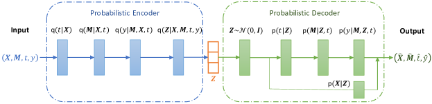
Figure 2. Illustration of the overall architecture of the networks for CMAVAE. The Probabilistic Encoder (blue part) takes the observables $({\bf X},{\bf M},t,y)$ as the input and encode the posterior distribution $q({\bf Z}|{\bf X},{\bf M},t,y)$. The Probabilistic Decoder (green part) takes the input of ${\bf Z}$ sampled from Gaussian prior distribution and decode the prior distributions for $({\bf X},{\bf M},t,y)$. Best viewed in colors.

4.1. Identifying Causal Mediation Effect

To recover ACME and ACDE from observational data, we take the expectation of CME and CDE under treatment $t$. First, we introduce the following assumption that validates the identification results:

Assumption 2 (The Proposed Assumption).

• There exists some latent variable ${\bf Z}$ that simultaneously deconfounds $T,{\bf M}$, and $Y$. Formally,

  (7) $${Y(t^{\prime},{\bf m}),{\bf M}(t)}\rotatebox[origin={c}]{90.0}{$\models$}T|{\bf Z}={\bf z},$$

  (8) $$Y(t^{\prime},{\bf m})\rotatebox[origin={c}]{90.0}{$\models$}{\bf M}(t)|T=t,{\bf Z}={\bf z}.$$

• There exists some observed variable ${\bf X}$ that approximates ${\bf Z}$;

• $p({\bf Z},{\bf X},{\bf M},t,y)$ can be approximately recovered from the observations $({\bf X},{\bf M},t,y)$ under Fig. 1.

The proposed assumption ensures that the HC ${\bf Z}$ can be (at least partially) estimated by covariates ${\bf X}$, $T$, ${\bf M}$ and $Y$. While HC is not necessarily always related to ${\bf X}$, there are many cases where this is possible (Louizos et al., 2017). Similar to previous literature (Cai and Kuroki, 2012) in causal inference in the presence of HC, the third assumption also implies that the causal graph $G$ and the corresponding joint distribution $p({\bf Z},{\bf X},{\bf M},t,y)$ are faithful to each other, i.e., the conditional independence in the joint distribution is also reflected in $G$, and vice versa (Spirtes et al., 2000).

Given observations (${\bf X},{\bf M},t,y$), ACME in Eq. (4) can then be reformulated as

(9) $$\begin{split}\overline{\delta}(t)&:=\mathbb{E}[CME({\bf x},t)],\text{with}\\ &CME({\bf x},t):=\mathbb{E}[y|{\bf X}={\bf x},T=t,{\bf M}(do(t^{\prime}=1))]\\ &-\mathbb{E}[y|{\bf X}={\bf x},T=t,{\bf M}(do(t^{\prime}=0))],\quad t=0,1.\end{split}$$

Based on previous results in (Louizos et al., 2017) and Pearl’s back-door adjustment formula (Pearl, 2012), we propose the following theorem:

Theorem 1.

If we estimate $p({\bf Z},{\bf X},{\bf M},t,y)$, then we recover CME and CDE under the causal graph in Fig. 1.

The proof can be seen in Appendix A. Theorem 1 connects the joint distribution $p({\bf Z},{\bf X},{\bf M},t,y)$ with causal effects in CMA. We recognize that the true distribution of $p({\bf Z},{\bf X},{\bf M},t,y)$ can only be approximately recovered using observational data. As noted in the Related Work section, literature in various research fields also provides support for using the joint distribution to study causal effects with HC. We do acknowledge the weakness of the approximated $p({\bf Z},{\bf X},{\bf M},t,y)$ in making conclusive causal claims, but they provide complementary advantages over conventional sequential ignorability assumptions in many aspects. Particularly noteworthy is that the observed covariates ${\bf X}$ should be related to ${\bf Z}$. For example, ${\bf X}$ is a “noisy” function of ${\bf Z}$ which is comprised of binary variables (Jernite et al., 2013). Next, we show how to approximate $p({\bf Z},{\bf X},{\bf M},t,y)$ from observations of $({\bf X},{\bf M},t,y)$ using deep latent variable models.

4.2. Causal Mediation Analysis Variational Auto-Encoder

Our approach–Causal Mediation Analysis with Variational Auto-Encoder (CMAVAE)–builds on Variational Auto-Encoder (VAE) (Kingma and Welling, 2013) that discovers ${\bf Z}$ in the latent space by variational inference. VAE makes smaller error in approximations and is robust against the noise of proxy variables. Here, we use VAEs to infer the complex non-linear relationships between ${\bf X}$ and $({\bf Z},{\bf M},t,y)$, and approximately recover $p({\bf Z},{\bf X},{\bf M},t,y)$. CMAVAE parameterizes the causal graph in Fig. 1 as a latent-variable model with neural network functions connecting the variables of interest. The objective function of VAE is then the reconstruction error of the observed $({\bf X},{\bf M},t,y)$ and the inferred $(\hat{{\bf X}},\hat{{\bf M}},\hat{t},\hat{y})$. Fig. 2. features the overall architecture design of CMAVAE. In the following descriptions of VAE, ${\bf x}_{i}$ denotes a feature vector of an input sample $i$, ${\bf m}_{i}$ is the mediator, $t_{i}$, $y_{i}$, and ${\bf z}_{i}$ denote the treatment status, outcome, and HC, respectively.

Let $D_{x}$, $D_{z}$ be the dimensions of ${\bf x}_{i}$ and of ${\bf z}_{i}$ respectively and each $f_{k}(\cdot),k\in\{1,2,3,4,5\}$ represents a neural network parameterized by its own parameters $\bm{\theta}_{k}$. We define

(10) $$p({\bf z}_{i})=\prod_{j=1}^{D_{z}}\mathcal{N}({\bf z}_{ij}|0,1);\quad p({\bf x}_{i}|{\bf z}_{i})=\prod_{j=1}^{D_{x}}p({\bf x}_{ij}|{\bf z}_{i});$$

(11) $$p(t_{i}|{\bf z}_{i})=\text{Bern}(\sigma(f_{1}({\bf z}_{i}))),$$

with $p({\bf x}_{ij}|{\bf z}_{i})$ being a probability distribution for the $j$-th covariate of ${\bf x}_{i}$ and $\sigma(\cdot)$ being the logistic function. For a continuous mediator and outcome, we parameterize the probability distribution as Gaussian distribution. The corresponding parameters are designed by using a similar architecture inspired by TARnet (Shalit et al., 2017). The details can be seen as follows:

(12) $$p({\bf m}_{i}|{\bf z}_{i},t_{i})=\mathcal{N}(\mu=\hat{\mu}_{1i},\sigma^{2}=\hat{\nu}_{1});$$

(13) $$p(y_{i}|{\bf m}_{i},{\bf z}_{i},t_{i})=\mathcal{N}(\mu=\hat{\mu}_{2i},\sigma^{2}=\hat{\nu}_{2}),$$

(14) $$\hat{\mu}_{1i}=t_{i}f_{2}({\bf z}_{i})+(1-t_{i})f_{3}({\bf z}_{i});$$

(15) $$\hat{\mu}_{2i}=t_{i}f_{4}({\bf z}_{i}\circ{\bf m}_{i})+(1-t_{i})f_{5}({\bf z}_{i}\circ{\bf m}_{i}).$$

$\hat{\nu}_{1}$ and $\hat{\nu}_{2}$ are predefined constant. We denote the concatenation of vectors as $\circ$. Then the posterior over ${\bf Z}$ can be approximated by

(16) $$q({\bf z}_{i}|{\bf x}_{i},{\bf m}_{i},y_{i},t_{i})=\prod_{j=1}^{D_{z}}\mathcal{N}(\mu_{j}=\overline{\mu}_{ij},\sigma^{2}_{j}=\overline{\sigma}^{2}_{ij});$$

(17) $$\overline{\bm{\mu}}_{i}=t_{i}\bm{\mu}_{t=0,i}+(1-t_{i})\bm{\mu}_{t=1,i};$$

(18) $$\overline{\bm{\sigma}}_{i}^{2}=t_{i}\bm{\sigma}^{2}_{t=0,i}+(1-t_{i})\bm{\sigma}^{2}_{t=1,i};$$

(19) $$\bm{\mu}_{t=0,i},\bm{\sigma}^{2}_{t=0,i}=g_{1}({\bf x}_{i}\circ y_{i}\circ{\bf m}_{i});$$

(20) $$\bm{\mu}_{t=1,i},\bm{\sigma}^{2}_{t=1,i}=g_{2}({\bf x}_{i}\circ y_{i}\circ{\bf m}_{i}),$$

where $g_{k}$ is a neural network with variational parameters $\bm{\phi}_{k}$ for $k\in\{1,2,...,7\}$. The objective function of VAEs is then:

(21) $$\begin{split}\mathcal{L}=\sum_{i=1}^{n}\mathbb{E}_{q({\bf z}_{i}|{\bf x}_{i},t_{i},{\bf m}_{i},y_{i})}[\log p({\bf z}_{i})+\log p({\bf x}_{i}|{\bf z}_{i})+\log p(t_{i}|{\bf z}_{i})\\ +\log p({\bf m}_{i}|{\bf z}_{i},t_{i})+\log p(y_{i}|{\bf m}_{i},{\bf z}_{i},t_{i})-\log q({\bf z}_{i}|{\bf x}_{i},{\bf m}_{i},y_{i},t_{i})].\end{split}$$

However, in the Encoder, we still need to infer $t$, ${\bf m}$ and $y$ for new subjects before inferring the posterior distribution over ${\bf z}$. Hence, we introduce three auxiliary distributions that predict $t_{i},{\bf m}_{i},y_{i}$ for new sample characterized by ${\bf x}_{i}$:

(22) $$q(t_{i}|{\bf x}_{i})=\text{Bern}(\pi=\sigma(g_{3}({\bf x}_{i})));$$

(23) $$q({\bf m}_{i}|{\bf x}_{i},t_{i})=\mathcal{N}(\mu=\overline{\mu}_{1i},\sigma^{2}=\overline{\nu}_{1});$$

(24) $$\overline{\mu}_{1i}=t_{i}g_{4}({\bf x}_{i})+(1-t_{i})g_{5}({\bf x}_{i}).$$

Similarly, we have

(25) $$q(y_{i}|{\bf x}_{i},{\bf m}_{i},t_{i})=\mathcal{N}(\mu=\overline{\mu}_{2i},\sigma^{2}=\overline{\nu}_{2});$$

(26) $$\overline{\mu}_{2i}=t_{i}g_{6}({\bf x}_{i}\circ{\bf m}_{i})+(1-t_{i})g_{7}({\bf x}_{i}\circ{\bf m}_{i}),$$

Here, $\overline{\nu}_{1}$ and $\overline{\nu}_{2}$ are predefined. The final loss is defined as

(27) $$\begin{split}\mathcal{F}&=\mathcal{L}+\sum_{i=1}^{n}(\log q({\bf m}_{i}={\bf m}_{i}^{*}|{\bf x}_{i}^{*},t_{i}^{*})+\\ \log q(t_{i}&=t_{i}^{*}|{\bf x}_{i}^{*})+\log q(y_{i}=y_{i}^{*}|{\bf x}_{i}^{*},{\bf m}_{i}^{*},t_{i}^{*})),\end{split}$$

where $y_{i}^{*},{\bf x}_{i}^{*},{\bf m}_{i}^{*},t_{i}^{*}$ are the observed values for the outcome, input, mediator, and treatment random variables in the training set.

5. Experiments

Evaluation in causal inference has been a long-standing challenge due to the lack of ground-truth effects (Guo et al., 2020; Cheng et al., 2022, 2019). For CMA, this is more challenging because both direct and indirect effects need to be specified, which cannot be achieved by randomized experiments. Therefore, CMA evaluation often has to rely on simulations (Huber et al., 2016; Imai et al., 2013). Here, we first conduct empirical evaluations using synthetic and semi-synthetic datasets, where real data is modified such that the true indirect and direct effects are known. We also perform a case study to show the application of CMAVAE in fair machine learning.

5.1. Experimental Settings

We used Tensorflow (Abadi et al., 2016) and Edward (Tran et al., 2016) to implement CMAVAE. Design of the neural network architecture is similar to that in (Shalit et al., 2017). For JOBS II data, unless otherwise specified, we used 5 hidden layers with size 100 and with ELU (Clevert et al., 2015) nonlinearities for the approximate posterior over the latent variables $q({\bf Z}|{\bf X},{\bf M},t,y)$, the generative model $p({\bf X}|{\bf Z})$, the mediator models $p({\bf M}|{\bf Z},t)$, $q({\bf M}|{\bf X},t)$ and the outcome models $p(Y|{\bf M},{\bf Z},t)$, $q(Y|{\bf M},{\bf X},t)$. One single hidden layer neural network with ELU nonlinearities is adopted to model $p(t|{\bf Z})$, $q(t|{\bf X})$. The dimension of the latent variable ${\bf Z}$ is set to 10. To prevent overfitting in the neural nets, we also applied a small weight decay term to all parameters with $\lambda=10^{-3}$. We optimized the objective function with Adam (Kingma and Ba, 2014) and a learning rate of $10^{-6}$. To estimate the mediators and outcomes, we averaged over 100 samples from the approximate posterior $q({\bf Z}|{\bf X})=\sum_{t}\int_{y}q({\bf Z}|t,y,{\bf X},{\bf M})q(y|t,{\bf X},{\bf M})q({\bf M}|t,{\bf X})q(t|{\bf X})dy$. More implementation details can be found in Appendix C.

Baselines include popular parametric methods LSEM (Baron and Kenny, 1986), LSEM-I (Imai et al., 2010), NEM-W, NEM-I (Lange et al., 2012), and semi-parametric methods IPW (Huber, 2014):

• LSEM (Baron and Kenny, 1986). A common framework for CMA. It is based on linear equations characterizing the outcome and the mediator.

• LSEM-I (Imai et al., 2010). An non-linear extension of LSEM with an interaction term between treatment and mediator.

• IPW (Huber, 2014; Huber et al., 2013). This approach is based on a common weighting strategy in causal inference, i.e.,IPW (Robins et al., 1994), to measure confounder effects and adjust analyses to remove the confounding bias.

• Natural Effect Models (NEM) (Lange et al., 2012). NEM are conditional mean models for counterfactuals in CMA. It directly models the direct and indirect effects by treating the task as a missing data problem. There are two approaches for data augmentation in NEM according to unobserved $(t,1-t)$ combinations – the weighting-based approach (NEM-W) and the imputing-based approach (NEM-I).

We used R package “mediation” for LSEM and LSEM-I, “causalweight” for IPW (the parameter trim was set to 0.05), and “medflex” for NEM-W, NEM-I. Evaluation metric is the absolute error of estimated ACDE $\overline{\zeta}(0)$, ACME $\overline{\delta}(1)$, and the total effect (ATE).

5.2. JOBS II Dataset

We first test CMAVAE on the real-world dataset JOBS II (Vinokur and Price, 1999), collected from a randomized field experiment that investigates the efficacy of a job training intervention on unemployed workers. Participants were randomly asked to attend the job skills workshops, i.e., the treatment group, or receive a booklet, i.e., the control group. The treatment group learned job hunting skills and coping strategies for confronting the setbacks in the job hunting process while the control group learned job hunting tips through a booklet. In follow-up interviews, the outcome – a continuous measure of depressive symptoms – was measured. Mediator $M$ is a continuous measure representing the job search self-efficacy. JOB II can be downloaded from R package “mediation” and the total sample size is 899. We further performed normalization on all continuous covariates and applied one-hot encoding to categorical covariates.

Table 1. Absolute errors for JOBS II data with 10% mediated ($\alpha$). $n=500,1000$ and $\eta=1,10$. (%)

ACME under treated ($\overline{\delta}(1)$)
Models	LSEM		LSEM-I		NEM-W		NEM-I		IPW		CMAVAE
$n$	500	1000	500	1000	500	1000	500	1000	500	1000	500	1000
$\eta=10$	0.7$\pm$.03	0.7$\pm$.02	0.9$\pm$.04	0.6$\pm$.02	0.3$\pm$.04	0.3$\pm$.01	0.6$\pm$.03	0.8$\pm$.01	0.6$\pm$.04	0.8$\pm$.02	0.2$\pm$.00	0.3$\pm$.00
$\eta=1$	0.1$\pm$.01	0.1$\pm$.01	0.0$\pm$.01	0.1$\pm$.01	0.0$\pm$.01	0.1$\pm$.01	0.0$\pm$.00	0.1$\pm$.01	0.0$\pm$.01	0.1$\pm$.01	0.1$\pm$.00	0.1$\pm$.00
ACDE under control ($\overline{\zeta}(0)$)
$\eta=10$	0.8$\pm$.07	2.0$\pm$.06	1.3$\pm$.07	1.6$\pm$.06	2.5$\pm$.06	1.2$\pm$.05	1.2$\pm$.06	1.8$\pm$.05	1.2$\pm$.06	0.2$\pm$.06	0.1$\pm$.00	0.0$\pm$.03
$\eta=1$	3.2$\pm$.08	0.3$\pm$.07	3.3$\pm$.08	0.0$\pm$.07	3.3$\pm$.08	0.3$\pm$.07	1.1$\pm$.03	0.2$\pm$.07	3.3$\pm$.08	0.3$\pm$.06	0.5$\pm$.02	0.4$\pm$.01
ATE ($\overline{\tau}$)
$\eta=10$	1.5$\pm$.06	1.2$\pm$.05	2.2$\pm$.05	1.0$\pm$.06	2.2$\pm$.06	0.8$\pm$.06	1.8$\pm$.05	0.9$\pm$.06	0.5$\pm$.05	1.0$\pm$.06	0.3$\pm$.01	0.3$\pm$.03
$\eta=1$	3.4$\pm$.08	0.2$\pm$.07	3.3$\pm$.08	0.1$\pm$.07	3.4$\pm$.08	0.2$\pm$.06	3.4$\pm$.03	0.1$\pm$.06	3.2$\pm$.07	0.2$\pm$.05	0.4$\pm$.02	0.3$\pm$.01

Table 2. Absolute errors for JOBS II data with 50% mediated ($\alpha$). $n=500,1000$ and $\eta=1,10$. (%)

ACME under treated ($\overline{\delta}(1)$)
Models	LSEM		LSEM-I		NEM-W		NEM-I		IPW		CMAVAE
$n$	500	1000	500	1000	500	1000	500	1000	500	1000	500	1000
$\eta=10$	1.3$\pm$.03	0.5$\pm$.03	0.9$\pm$.03	0.6$\pm$.03	0.9$\pm$.04	1.2$\pm$.03	0.2$\pm$.03	0.4$\pm$.03	0.2$\pm$.03	0.4$\pm$.03	0.0$\pm$.00	0.1$\pm$.00
$\eta=1$	0.2$\pm$.01	0.0$\pm$.01	0.1$\pm$.01	0.0$\pm$.01	0.2$\pm$.00	0.1$\pm$.00	0.2$\pm$.00	0.1$\pm$.01	0.1$\pm$.01	0.0$\pm$.01	0.1$\pm$.00	0.1$\pm$.00
ACDE under control ($\overline{\zeta}(0)$)
$\eta=10$	0.9$\pm$.07	0.1$\pm$.04	0.6$\pm$.06	0.1$\pm$.04	0.2$\pm$.07	0.5$\pm$.04	0.1$\pm$.06	0.1$\pm$.04	0.7$\pm$.07	0.2$\pm$.05	0.3$\pm$.01	0.1$\pm$.00
$\eta=1$	0.4$\pm$.01	0.4$\pm$.01	0.1$\pm$.10	0.3$\pm$.10	0.5$\pm$.10	0.4$\pm$.04	0.1$\pm$.10	0.3$\pm$.04	0.3$\pm$.10	0.2$\pm$.04	0.1$\pm$.00	0.1$\pm$.00
ATE ($\overline{\tau}$)
$\eta=10$	0.4$\pm$.05	0.6$\pm$.03	0.3$\pm$.05	0.8$\pm$.03	0.7$\pm$.05	0.7$\pm$.01	0.1$\pm$.05	0.5$\pm$.03	0.9$\pm$.05	0.2$\pm$.04	0.3$\pm$.01	0.0$\pm$.01
$\eta=1$	0.2$\pm$.10	0.4$\pm$.04	0.1$\pm$.09	0.3$\pm$.04	0.2$\pm$.10	0.3$\pm$.04	0.3$\pm$.10	0.3$\pm$.04	0.2$\pm$.10	0.2$\pm$.04	0.0$\pm$.01	0.2$\pm$.01

Simulation. To obtain the ground truth for direct and indirect effects, we used a simulation approach similar to (Huber et al., 2013, 2016). Specifically, we first estimate probit specifications in which we regress (1) $T$ on ${\bf X}$ and (2) $M$ on $T$ and ${\bf X}$ using the entire JOBS II data. As the mediator in JOBS II is a continuous variable in the range of [1,5], we apply the Indicator function $I$ to $M_{i}$: $I\{M_{i}\geq 3\}$. The output of $I(\cdot)$ is 1, i.e., mediated, if the argument is satisfied and 0, i.e., nonmediated, otherwise. All observations with $T=1$ and $I(M_{i})=1$ (or both) are then discarded. We draw independent Monte Carlo samples with replacement ${\bf X}^{\prime}$ from the original dataset of the nontreated and nonmediated (Huber et al., 2016). The next step simulates the (pseudo-)treatment:

(28) $$T_{i}=I\{{\bf X}^{\prime}_{i}\hat{\beta}_{pop}+U_{i}>0\},$$

where $\hat{\beta}_{pop}$ are the probit coefficient estimates of the treatment model using original data. $U_{i}\sim\mathcal{N}(0,1)$ denotes the environment noise. The (pseudo-)mediator is simulated by

(29) $$M_{i}=\eta(T_{i}\hat{\gamma}_{pop}+{\bf X}_{i}^{\prime}\hat{\omega}_{pop})+\alpha+V_{i},$$

where $\hat{\gamma}_{pop}$ and $\hat{\omega}_{pop}$ are the probit coefficient estimates on $T$ and ${\bf X}$ of the mediator model using original data and $V_{i}\sim\mathcal{N}(0,1)$ denotes the Gaussian noise. $\eta$ gauges the magnitude of selection into the mediator. Following (Huber et al., 2016), we consider $\eta=1$ (normal selection) and $\eta=10$ (strong selection). $\alpha$ determines the shares of mediated individuals. In our simulations, we set $\alpha$ such that either 10% or 50% of the observations are mediated ($I(M_{i})=1$). With this particular simulation design, we obtain the true direct, indirect and total effect of zero. This is because all observations including the pseudo-treated/mediated ones are drawn from the population neither treated nor mediated. Combinations of the sample size, strength of selection into the mediator and share of mediated observations yield all in all 8 different data generating processes (DGPs). We use 80% of data for training and keep the ratio of number of treated to controlled in the training and test datasets same.

Table 3. Performance comparisons using JOBS II data with 50% mediated ($\alpha$), $n=500$, and $\eta=1$. The data is generated with the injection of different levels of proxy noise.

(a) Results for estimating ACME ($\overline{\delta}(1)$). (%)

Proxy noise	$0.1$	$0.2$	$0.3$	$0.4$	$0.5$
LSEM	0.2	0.1	0.2	0.2	0.5
LSEM-I	0.2	0.2	0.3	0.2	0.8
IPW	0.2	0.2	0.2	0.2	0.8
NEM-W	0.2	0.1	0.1	0.2	0.5
NEM-I	0.2	0.1	0.2	0.2	0.5
CMAVAE	0.1	0.1	0.2	0.2	0.2

(b) Results for estimating ACDE ($\overline{\zeta}(0)$). (%)

Proxy noise	$0.1$	$0.2$	$0.3$	$0.4$	$0.5$
LSEM	2.9	2.8	4.6	5.0	5.9
LSEM-I	3.4	3.1	5.1	5.2	6.0
IPW	3.7	2.8	4.7	5.3	5.6
NEM-W	3.4	2.8	4.5	5.2	5.7
NEM-I	3.4	2.7	4.6	5.3	5.8
CMAVAE	1.3	1.0	1.3	1.5	3.4

(c) Results for estimating ATE ($\overline{\tau}$). (%)

Proxy noise	$0.1$	$0.2$	$0.3$	$0.4$	$0.5$
LSEM	3.0	2.9	4.6	5.0	6.0
LSEM-I	3.5	3.2	5.2	5.1	5.9
IPW	3.8	2.9	4.7	5.2	5.8
NEM-W	3.5	2.8	4.5	5.2	6.0
NEM-I	3.5	2.8	4.6	5.2	6.0
CMAVAE	1.3	1.0	1.3	1.5	3.6

Table 4. Performance comparisons using JOBS II data with 10% mediated ($\alpha$), $n=500$, and $\eta=1$. The data is generated with the injection of different levels of proxy noise.

(a) Results for estimating ACME ($\overline{\delta}(1)$). (%)

Proxy noise	$0.1$	$0.2$	$0.3$	$0.4$	$0.5$
LSEM	0.2	0.2	0.1	0.1	0.3
LSEM-I	0.2	0.2	0.1	0.2	0.3
IPW	0.2	0.3	0.1	0.2	0.2
NEM-W	0.2	0.2	0.1	0.1	0.2
NEM-I	0.2	0.2	0.1	0.1	0.3
CMEVAE	0.1	0.1	0.1	0.1	0.1

(b) Results for estimating ACDE ($\overline{\zeta}(0)$). (%)

Proxy noise	$0.1$	$0.2$	$0.3$	$0.4$	$0.5$
LSEM	3.4	3.1	4.0	4.4	3.6
LSEM-I	3.1	3.6	4.8	4.0	3.2
IPW	3.7	4.0	4.6	4.1	2.8
NEM-W	3.0	3.4	4.3	4.4	3.3
NEM-I	3.0	3.6	4.3	4.4	3.3
CMEVAE	1.6	1.1	1.6	1.3	1.5

(c) Results for estimating ATE ($\overline{\tau}$). (%)

Proxy noise	$0.1$	$0.2$	$0.3$	$0.4$	$0.5$
LSEM	3.4	3.0	4.0	4.4	3.5
LSEM-I	3.1	3.5	4.8	4.0	3.2
IPW	3.7	3.9	4.5	4.1	2.9
NEM-W	3.0	3.3	4.2	4.4	3.3
NEM-I	3.0	3.4	4.3	4.4	3.2
CMEVAE	1.7	1.0	1.7	1.3	1.6

Results. Each set of experiment was conducted 10 replications and we report the averaged results as well as the standard deviations for the 8 DGPs in Table 1-2. Note when the best mean of multiple models are equal, we highlight results with the least standard deviations. We can draw following conclusions from our observations:

• CMAVAE mostly outperforms the baselines w.r.t. the accuracy of estimating ACDE, ACME and ATE. For instance, in Table 1 where $\eta=10$, $n=500$, CMAVAE presents the least absolute error in all three estimations and the improvement is significant. Specifically, compared to the best baselines (i.e., LSEM and IPW), CMAVAE can reduce the error of estimating ACDE and ATE by 87.5% and 40.0%, respectively. The results manifest the effectiveness of the proposed framework.

• CMAVAE also achieves smaller standard deviations compared to other models. Its robustness, in part, benefits from the joint estimation of the unknown latent space of HC and the causal effects in CMA. The baselines, however, mostly present much larger standard deviations.

• For simulation parameters, strong selection of mediators ($\eta$) leads to larger bias in the estimation of ACME compared to normal selection. Larger $\alpha$ (more targets are mediated) roughly leads to larger error in ACME estimation and smaller error in ACDE estimation. Compared to baselines, CMAVAE shows more robust performance to the changes of parameters for simulation. This result further illustrates the importance as well as the challenges of decomposing the total effect in order to understand the underlying causal mechanism.

Varying Proxy Noise. To further illustrate the effectiveness and robustness of CMAVAE, we introduce a new variable $p_{c}$, denoting the noise level of the proxies. Specifically, a larger $p_{c}$ indicates that we have less direct access to information of HC. Following a similar data generating procedure in (Louizos et al., 2017), we identify HC in JOBS II as a single variable that is highly correlated with the outcome (depressive symptoms) – PRE-DEPRESS, the pre-treatment level of depression. We then simulate proxies of PRE-DEPRESS by manually injecting noise into PRE-DEPRESS. In particular, we first simulate treatment $t_{i}$ using ${\bf x}_{i}$ and the confounder PRE-DEPRESS ${\bf z}_{i}$:

(30) $$t_{i}|{\bf x}_{i},{\bf z}_{i}\sim\text{Bern}\big{(}\sigma(w_{x}^{T}{\bf x}+w_{z}(\frac{{\bf z}}{3}-0.3))\big{)},$$

where $w_{x}\sim\mathcal{N}(0,0.1)$, $w_{z}\sim\mathcal{N}(5,0.1)$. To create the proxies for PRE-DEPRESS, we binned the samples into 3 groups based on their PRE-DPRESS values and applied one-hot encoding, which is replicated 3 times. We use three replications as previous studies have suggested that three independent views of a latent feature are what is needed to ensure its recover (Kruskal, 1976; Allman et al., 2009; Anandkumar et al., 2014). We then randomly and independently flip each of these 9 binary features with probability $p_{c}$. We let $p_{c}$ vary from 0.1 to 0.5 with an increment of 0.1. $p_{c}=0.5$ indicates the proxies have no direct information of the confounder. In this experiment, we set $n=500$, $\eta=1$, and examine both $\alpha=0.5$ (50% samples are mediated) and $\alpha=0.1$. Results averaged over 10 replications are shown in Table 3(c)-4(c).

We see from the results that CMEVAE mostly achieves the best performance when varying $p_{c}$. The improvement over baseline models w.r.t. ACDE and ATE is significant, see e.g., $p_{c}=0.5$ in Table 3(c)(b)-(c). In addition, CMAVAE presents relatively more robust results with different proxy noise compared to other models, see, e.g., Table 4(c)(a)-(c). This is because CMAVAE can infer a cleaner latent representation from the noisy proxies (Louizos et al., 2017). When there are 50% samples are mediated, i.e., $\alpha=0.5$, performance of all models roughly degrades with an increasing $p_{c}$. Models are more robust to increasing proxy noise when fewer samples are mediated, i.e., $\alpha=0.1$, in part because i) models can focus on the task of estimating the direct effect; and ii) the pre-treatment depression level has a stronger impact on the mediator (job search self-efficacy) than the treatment (job training or booklets) as we can see the performance degradation w.r.t. ACME when $p_{c}$ increases in both experiments. Overall, CMAVAE is more robust to the proxy noise than conventional methods for CMA, achieving high precision even the proxy cannot provide any useful information of HC at noise level 0.5.

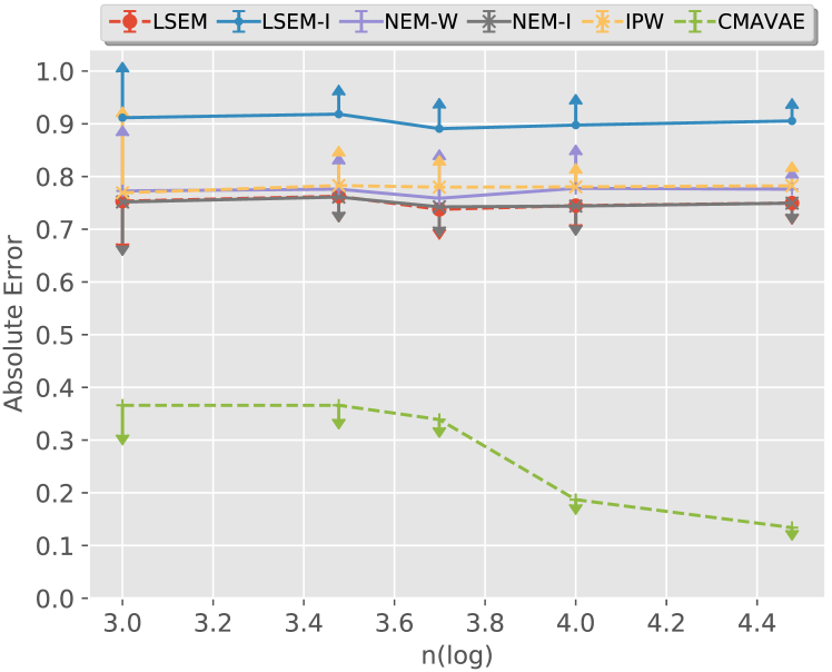
(a) Estimation of ACME under treated.

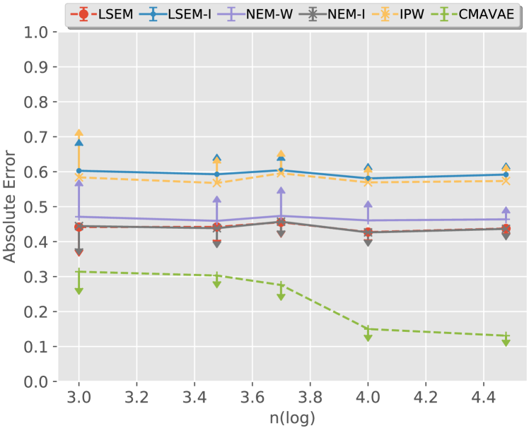
(b) Estimation of ACDE under control.

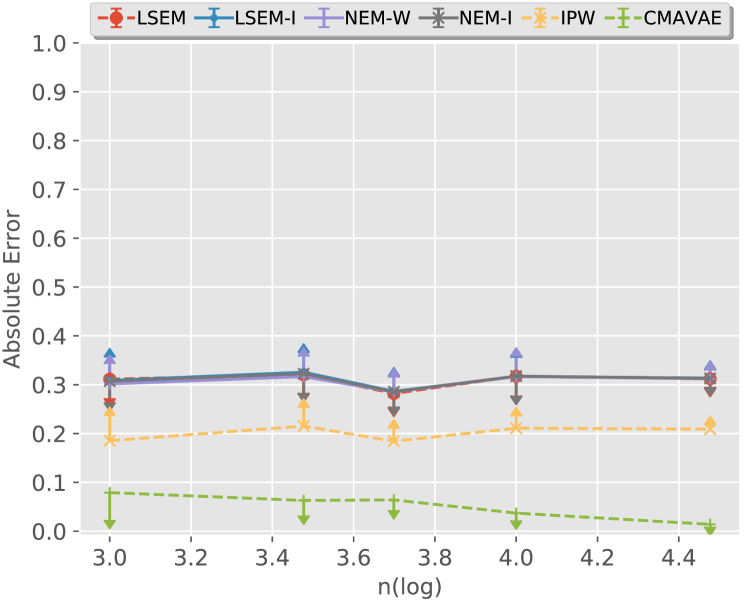
(c) Estimation of ATE.

Figure 3. Absolute errors of the estimated ACME, ACDE, ATE on synthetic samples simulated from the data generative process (Eq. (31)).

5.3. Synthetic Experiments

Suppose that ${\bf X}$ are the attributes of customers, ${\bf M}$ is the engagement of users in organic search, $T$ denotes whether a customer is using the new recommendation module $(T=1)$ or not $(T=0)$, $Y$ is the conversion rate, and ${\bf Z}$ is the HC. We define ${\bf Z}$, ${\bf M}$, ${\bf X}$, $T$ and $Y$ as

(31) $$\begin{split}{\bf z}_{i}\sim\text{Bern}(0.5);\\ {\bf x}_{i}|{\bf z}_{i}\sim\mathcal{N}({\bf z}_{i},25{\bf z}_{i}+9(1-{\bf z}_{i}));\\ t_{i}|{\bf z}_{i}\sim\text{Bern}(0.75{\bf z}_{i}+0.25(1-{\bf z}_{i}));\\ {\bf m}_{i}|{\bf z}_{i},t_{i}\sim 0.5{\bf z}_{i}+0.5t_{i}\bm{\kappa}_{i}+{\bf e}_{1};\\ y_{i}|{\bf z}_{i},t_{i},{\bf m}_{i}\sim{\bf c}{\bf z}_{i}+t_{i}+{\bf m}_{i}+0.5t_{i}{\bf m}_{i}+{\bf e}_{2},\end{split}$$

where $\bm{\kappa}_{i}=\frac{1}{1+\exp(-(1+0.2{\bf z}_{i}))}$ models the influence of using new recommendation module on user engagement through the HC ${\bf z}_{i}$. We let ${\bf c}\sim\mathcal{N}(0,1)$ be the scaling factor and ${\bf e}_{1},{\bf e}_{2}\sim\mathcal{N}(0,1)$ represent the Gaussian noise. This data generating process explicitly introduces HC between $t$ and ${\bf m}$, $t$ and $y$, and ${\bf m}$ and $y$ as they all hinge on the mixture assignment ${\bf z}$ for ${\bf x}$. As the sequential ignorability assumption has been violated, we expect that baselines may not accurately estimate ACME, ACDE and ATE. We model ${\bf z}$ as a 5-dimensional continuous variable following the Gaussian distribution to investigate the robustness of CMAVAE w.r.t. model misspecification. We evaluate across sample sizes $n\in\{1000,3000,5000,10000,30000\}$ and present the mean and standard deviation of each approach in Fig. 3.

Results. CMAVAE achieves significantly less error and variance than the baseline models across various settings although we purposely misspecified the latent model. Specifically, the relative improvement over baselines is the largest for estimating ACME, smaller for ACDE, and the least for ATE. This implies that estimated ACDE and ACME deviate from the ground truth in opposite directions, yielding a total effect that is closer to the ground truth. Additionally, the improvement w.r.t. the averages of estimated effects and the corresponding standard deviations becomes more significant when the sample size increases, showing the promises of using big-data for causal inference in the presence of proxies for HC (Louizos et al., 2017).

5.4. Application in Causal Fairness Analysis

In addition to the simulation-based evaluation, we apply CMAVAE to the real-world example described in Example 2. This experiment illustrates how CMAVAE can help detect and interpret discrimination in machine learning from a causal perspective. In particular, we partition discrimination into two components – direct and indirect discrimination (Council et al., 2004). We use the benchmark UCI Adult dataset (Dua and Graff, 2017) where the sensitive attribute Gender is the treatment, Occupation the mediator, and Income ($>50K,\leq 50K$) the outcome (Zhang and Bareinboim, 2018). All other demographic covariates (e.g., marital status) are used as the proxies of HC. In comparison, we employ the statistical definition of fairness – demographic disparity (DP) (Dwork et al., 2012) – and Logistic Regression as the classifier for its interpretability and simplicity. Dealing in correlations, DP requires the outcome to be independent of the sensitive attributes, i.e., $P(\hat{Y}|T=0)=P(\hat{Y}|T=1)$. We report results for ACME, ACDE, ATE, and DP in Fig. 4 to show a bird’s-eye view of (1) how gender might affect the annual income directly (ACDE) and indirectly (ACME); (2) the differences of the discrimination measure between statistical and causal fairness (ATE and DP). Note that “ATE” under statistical fairness is the estimated coefficient of gender in the classifier and it cannot be split into direct and indirect effects. For CMAVAE, ATE=0 denotes non-discrimination. As we cannot know the ground-truth causal effects of gender on income, we only show the ground truth of DP calculated with true $Y$.

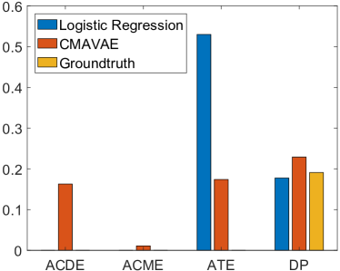
Figure 4. Comparisons of statistical and causal fairness analyses.

We observe that (1) both the “ATE” of gender for logistic regression and the ATE for CMAVAE are positive, indicating that there is potential discrimination against female employees. We can reach the similar conclusion from the results of DP; (2) based on CMAVAE results, a small part of the discrimination can be attributed to the indirect influence from occupation which is also affected by gender. We cannot get such information from statistical fairness; and (3) under statistical fairness notion, logistic regression presents closer DP to the ground truth. As DP relies on the accuracy of inferred $Y$, a better results from logistic regression is expected because highly predictive yet correlated information were removed from CMAVAE. Of particular interest is the contradictory results for ATE and DP: under causal fairness measure, “ATE” of gender for logistic regression is significantly larger than ATE for CMAVAE whereas the results are opposite under statistical fairness measure DP. This signals the inherent differences between causal and statistical fairness notions. Future research on the comparisons is warranted.

6. Conclusions & Future Work

This work studies an important causal inference problem that seeks to break down the total effect of a treatment into direct and indirect causal effects. When direct intervention on the mediator is not possible, CMA shows its potentials to reveal the underlying causal mechanism involved with treatment, mediator, and outcome. When applied to observational data, CMA relies on the sequential ignorability assumption – confounder bias can be controlled for by the observable covariates – that is often unverifiable in practice. This work circumvents the strong assumption and studies CMA in the presence of HC. To achieve the goal, we approximate HC by incorporating proxy variables that are easier to measure. The proposed approach CMAVAE draws connections between conventional CMA and recent advances in deep latent-variable models to simultaneously estimate HC and causal effects. Experimental results show the efficacy and potential applications of our approach.

This study opens promising future directions. First, we plan to investigate the influence of proxy variables on estimating ACME and ACDE separately. The empirical evaluations in Sec. 5 suggests that there might be a trade-off between these two tasks. We may further design a weighting strategy to balance between ACME and ACDE, increasing model’s flexibility in solving different tasks. In addition, we would like to extend this work to settings where multiple mediators are of particular interest. To apply CMAVAE into real-life applications such as clinical trials and recommendation systems, one needs to be aware of the scientific context of that specific scenario in order to maximize the performance of CMAVAE.

Appendix A Proof of Theorem 1

Proof. The key is to show that $p(y|{\bf X},{\bf M}(do(T=t^{\prime})),t)$ is identifiable. We have

(32) $$\begin{split}p(y|{\bf X},{\bf M}(do(T=t^{\prime})),t)=\\ \int_{{\bf Z}}p(y|{\bf X},{\bf M}(do(T=t^{\prime})),t,{\bf Z})p({\bf Z}|{\bf X},{\bf M}(do(T=t^{\prime})),t)d{\bf Z}\\ {=}\int_{{\bf Z}}p(y|{\bf X},{\bf M}(t^{\prime}),t,{\bf Z})p({\bf Z}|{\bf X},{\bf M}(t^{\prime}),t)d{\bf Z},\end{split}$$

where the second equality holds by applying the do-calculus rule to the causal graph in Fig.1. The final expression in Eq. (32) can be identified from the distribution $p({\bf Z},{\bf X},{\bf M},t,y)$. Similarly, we can prove that $p(y|{\bf X},{\bf M}(t),do(T=t^{\prime}))$ for ACDE is also identifiable given the joint probability distribution $p({\bf Z},{\bf X},{\bf M},t,y)$:

(33) $$\begin{split}\overline{\zeta}(t)&:=\mathbb{E}[CDE({\bf x},t)],\text{with}\\ CDE({\bf x},t)&:=\mathbb{E}[y|{\bf X}={\bf x},do(t^{\prime}=1),{\bf M}(T=t))]\\ &-\mathbb{E}[y|{\bf X}={\bf x},do(t^{\prime}=0),{\bf M}(T=t)],\quad t=0,1.\end{split}$$

Table 5. Details of the parameter settings in proposed models for both simulation data and real-world datasets.

Parameter	Simulation	JOBS II	Adult
Reps	10	10	1
Epoch	100	100	150
Embed_Size	5	10	10
Layer_Size	100	100	100
Batch_Size	100	32	1024
$lr$	1e-4	1e-6	1e-5
n_layers	3	5	2
$\lambda$	1e-4	1e-3	1e-3
$L$	100	100	1000

Appendix B CMAVAE in Binary Cases

With binary mediator and outcome, we first define

(34) $$p({\bf z}_{i})=\prod_{j=1}^{D_{z}}\mathcal{N}({\bf z}_{ij}|0,1);\quad p({\bf x}_{i}|{\bf z}_{i})=\prod_{j=1}^{D_{x}}p({\bf x}_{ij}|{\bf z}_{i});$$

(35) $$p(t_{i}|{\bf z}_{i})=\text{Bern}(\sigma(f_{1}({\bf z}_{i}))),$$

CMAVAE can then be formulated as follows:

(36) $$p({\bf m}_{i}|{\bf z}_{i},t_{i})=\text{Bern}(\pi=\hat{\pi}_{1i});$$

(37) $$p(y_{i}|{\bf m}_{i},{\bf z}_{i},t_{i})=\text{Bern}(\pi=\hat{\pi}_{2i}),$$

where

(38) $$\hat{\pi}_{1i}=\sigma(t_{i}f_{2}({\bf z}_{i})+(1-t_{i})f_{3}({\bf z}_{i}));$$

(39) $$\hat{\pi}_{2i}=\sigma(t_{i}f_{4}({\bf z}_{i}\circ{\bf m}_{i})+(1-t_{i})f_{5}({\bf z}_{i}\circ{\bf m}_{i})).$$

Then the posterior over ${\bf Z}$ can be approximated by

(40) $$q({\bf z}_{i}|{\bf x}_{i},{\bf m}_{i},y_{i},t_{i})=\prod_{j=1}^{D_{z}}\mathcal{N}(\mu_{j}=\overline{\mu}_{ij},\sigma^{2}_{j}=\overline{\sigma}^{2}_{ij});$$

(41) $$\overline{\bm{\mu}}_{i}=t_{i}\bm{\mu}_{t=0,i}+(1-t_{i})\bm{\mu}_{t=1,i};$$

(42) $$\overline{\bm{\sigma}}_{i}^{2}=t_{i}\bm{\sigma}^{2}_{t=0,i}+(1-t_{i})\bm{\sigma}^{2}_{t=1,i};$$

(43) $$\bm{\mu}_{t=0,i},\bm{\sigma}^{2}_{t=0,i}=g_{1}({\bf x}_{i}\circ y_{i}\circ{\bf m}_{i});$$

(44) $$\bm{\mu}_{t=1,i},\bm{\sigma}^{2}_{t=1,i}=g_{2}({\bf x}_{i}\circ y_{i}\circ{\bf m}_{i}),$$

The objective function of VAEs is then:

(45) $$\begin{split}\mathcal{L}=\sum_{i=1}^{n}\mathbb{E}_{q({\bf z}_{i}|{\bf x}_{i},t_{i},{\bf m}_{i},y_{i})}[\log p({\bf z}_{i})+\log p({\bf x}_{i}|{\bf z}_{i})+\log p(t_{i}|{\bf z}_{i})\\ +\log p({\bf m}_{i}|{\bf z}_{i},t_{i})+\log p(y_{i}|{\bf m}_{i},{\bf z}_{i},t_{i})-\log q({\bf z}_{i}|{\bf x}_{i},{\bf m}_{i},y_{i},t_{i})].\end{split}$$

However, in the Encoder, we still need to infer the treatment assignment $t$, mediator ${\bf m}$, and outcome $y$ for new subjects before inferring the posterior distribution over ${\bf z}$. As a result, we introduce three auxiliary distributions that seek to predict $t_{i},{\bf m}_{i},y_{i}$ for new samples with covariates ${\bf x}_{i}$. They are

(46) $$q(t_{i}|{\bf x}_{i})=\text{Bern}(\pi=\sigma(g_{3}({\bf x}_{i})));$$

(47) $$q({\bf m}_{i}|{\bf x}_{i},t_{i}) =\text{Bern}(\pi=\overline{\pi}_{1i}),$$

where

(48) $$\overline{\pi}_{1i}=\sigma(t_{i}g_{4}({\bf x}_{i})+(1-t_{i})g_{5}({\bf x}_{i})).$$

Similarly, we have

(49) $$q(y_{i}|{\bf x}_{i},{\bf m}_{i},t_{i}) =\text{Bern}(\pi=\overline{\pi}_{2i}),$$

where

(50) $$\overline{\pi}_{2i}=\sigma(t_{i}g_{6}({\bf x}_{i}\circ{\bf m}_{i})+(1-t_{i})g_{7}({\bf x}_{i}\circ{\bf m}_{i})).$$

The final loss is defined as

(51) $$\begin{split}\mathcal{F}&=\mathcal{L}+\sum_{i=1}^{n}(\log q({\bf m}_{i}={\bf m}_{i}^{*}|{\bf x}_{i}^{*},t_{i}^{*})+\\ \log q(t_{i}&=t_{i}^{*}|{\bf x}_{i}^{*})+\log q(y_{i}=y_{i}^{*}|{\bf x}_{i}^{*},{\bf m}_{i}^{*},t_{i}^{*})),\end{split}$$

where $y_{i}^{*},{\bf x}_{i}^{*},{\bf m}_{i}^{*},t_{i}^{*}$ are the observed values for the outcome, input, mediator and treatment random variables in the training set.

Appendix C Reproducibility

In this section, we provide more details of the experimental setting and configuration for reproducibility purpose.

Our proposed models were implemented in Python library Tensorflow (Abadi et al., 2016) and Edward (Tran et al., 2016). Code for data simulation and all baselines is written in R. We detail the parameter settings of the proposed models for simulation data, JOBS II data, and the Adult data for causal fair analysis in Table 5. The descriptions of the major parameters are introduced below:

• Reps: the number of replications each set of experiments runs. The parameters used are fixed, but each replication of the generated data can be different.

• Epoch: one Epoch is when an entire dataset is passed forward and backward through the neural network only once.

• Embed_Size: the dimensions of the latent variable $Z$.

• Layer_Size: the output size of every layer.

• Batch_Size: total number of training examples present in a single batch.

• $lr$: the learning rate.

• n_layers: the number of hidden layers.

• $\lambda$: the hyperparameter for weight decay.

• $L$: the number of samples drawn from the posterior distribution to estimate mediator and outcome.

References

- (1)
- Abadi et al. (2016) Martín Abadi, Ashish Agarwal, Paul Barham, Eugene Brevdo, Zhifeng Chen, Craig Citro, Greg S Corrado, Andy Davis, Jeffrey Dean, Matthieu Devin, et al. 2016. Tensorflow: Large-scale machine learning on heterogeneous distributed systems. arXiv preprint arXiv:1603.04467 (2016).
- Allman et al. (2009) Elizabeth S Allman, Catherine Matias, John A Rhodes, et al. 2009. Identifiability of parameters in latent structure models with many observed variables. The Annals of Statistics 37, 6A (2009), 3099–3132.
- Anandkumar et al. (2014) Animashree Anandkumar, Rong Ge, Daniel Hsu, Sham M Kakade, and Matus Telgarsky. 2014. Tensor decompositions for learning latent variable models. JMLR 15 (2014), 2773–2832.
- Angrist and Pischke (2008) Joshua D Angrist and Jörn-Steffen Pischke. 2008. Mostly harmless econometrics: An empiricist’s companion. Princeton university press.
- Baron and Kenny (1986) Reuben M Baron and David A Kenny. 1986. The moderator–mediator variable distinction in social psychological research: Conceptual, strategic, and statistical considerations. JPSP 51, 6 (1986), 1173.
- Cai and Kuroki (2012) Zhihong Cai and Manabu Kuroki. 2012. On identifying total effects in the presence of latent variables and selection bias. arXiv preprint arXiv:1206.3239 (2012).
- Cheng et al. (2019) Lu Cheng, Ruocheng Guo, Raha Moraffah, K Selçuk Candan, Adrienne Raglin, and Huan Liu. 2019. A practical data repository for causal learning with big data. In International Symposium on Benchmarking, Measuring and Optimization. Springer, 234–248.
- Cheng et al. (2022) Lu Cheng, Ruocheng Guo, Raha Moraffah, Paras Sheth, K. Selçuk Candan, and Huan Liu. 2022. Evaluation Methods and Measures for Causal Learning Algorithms. IEEE TAI (2022).
- Clevert et al. (2015) Djork-Arné Clevert, Thomas Unterthiner, and Sepp Hochreiter. 2015. Fast and accurate deep network learning by exponential linear units (elus). arXiv preprint arXiv:1511.07289 (2015).
- Council et al. (2004) National Research Council et al. 2004. Measuring racial discrimination. National Academies Press.
- Dua and Graff (2017) Dheeru Dua and Casey Graff. 2017. UCI Machine Learning Repository. http://archive.ics.uci.edu/ml
- Dwork et al. (2012) Cynthia Dwork, Moritz Hardt, Toniann Pitassi, Omer Reingold, and Richard Zemel. 2012. Fairness through awareness. In Proceedings of the 3rd innovations in theoretical computer science conference. 214–226.
- Frost (1979) Peter A Frost. 1979. Proxy variables and specification bias. Rev. Econ. Stat. (1979), 323–325.
- Greenland and Lash (2011) Sander Greenland and Timothy L Lash. 2011. Bias analysis. International Encyclopedia of Statistical Science 2 (2011), 145–148.
- Griliches and Hausman (1986) Zvi Griliches and Jerry A Hausman. 1986. Errors in variables in panel data. J. Econom. 31, 1 (1986), 93–118.
- Guo et al. (2020) Ruocheng Guo, Lu Cheng, Jundong Li, P Richard Hahn, and Huan Liu. 2020. A survey of learning causality with data: Problems and methods. ACM Computing Surveys (CSUR) 53, 4 (2020), 1–37.
- Huber (2014) Martin Huber. 2014. Identifying causal mechanisms (primarily) based on inverse probability weighting. Journal of Applied Econometrics 29, 6 (2014), 920–943.
- Huber et al. (2016) Martin Huber, Michael Lechner, and Giovanni Mellace. 2016. The finite sample performance of estimators for mediation analysis under sequential conditional independence. JBES 34, 1 (2016), 139–160.
- Huber et al. (2013) Martin Huber, Michael Lechner, and Conny Wunsch. 2013. The performance of estimators based on the propensity score. J. Econom. 175, 1 (2013), 1–21.
- Hyman (1955) Herbert Hiram Hyman. 1955. SURVEY DESIGN AND ANALYSIS: PRINCIPLES, CASES, AND PROCEDURES.. (1955).
- Imai et al. (2010) Kosuke Imai, Luke Keele, and Dustin Tingley. 2010. A general approach to causal mediation analysis. Psychological methods 15, 4 (2010), 309.
- Imai et al. (2013) Kosuke Imai, Dustin Tingley, and Teppei Yamamoto. 2013. Experimental designs for identifying causal mechanisms. Statistics in Society 176, 1 (2013), 5–51.
- James et al. (1982) Lawrence James, S Mulaik, and Jeanne M Brett. 1982. Causal analysis: Assumptions, models, and data. (1982).
- Jernite et al. (2013) Yacine Jernite, Yonatan Halpern, and David Sontag. 2013. Discovering hidden variables in noisy-or networks using quartet tests. In NIPS. 2355–2363.
- Judd and Kenny (1981) Charles M Judd and David A Kenny. 1981. Process analysis: Estimating mediation in treatment evaluations. Evaluation review 5, 5 (1981), 602–619.
- Keele (2015) Luke Keele. 2015. Causal mediation analysis: warning! Assumptions ahead. AJE 36, 4 (2015), 500–513.
- Kingma and Ba (2014) Diederik P Kingma and Jimmy Ba. 2014. Adam: A method for stochastic optimization. arXiv preprint arXiv:1412.6980 (2014).
- Kingma and Welling (2013) Diederik P Kingma and Max Welling. 2013. Auto-encoding variational bayes. arXiv preprint arXiv:1312.6114 (2013).
- Kolenikov and Angeles (2009) Stanislav Kolenikov and Gustavo Angeles. 2009. Socioeconomic status measurement with discrete proxy variables: Is principal component analysis a reliable answer? Review of Income and Wealth 55, 1 (2009), 128–165.
- Kruskal (1976) Joseph B Kruskal. 1976. More factors than subjects, tests and treatments: an indeterminacy theorem for canonical decomposition and individual differences scaling. Psychometrika 41, 3 (1976), 281–293.
- Lange et al. (2012) Theis Lange, Stijn Vansteelandt, and Maarten Bekaert. 2012. A simple unified approach for estimating natural direct and indirect effects. Am. J. Epidemiol. 176, 3 (2012), 190–195.
- Louizos et al. (2017) Christos Louizos, Uri Shalit, Joris M Mooij, David Sontag, Richard Zemel, and Max Welling. 2017. Causal effect inference with deep latent-variable models. In NIPS. 6446–6456.
- MacKinnon (2012) David MacKinnon. 2012. Introduction to statistical mediation analysis. Routledge.
- MacKinnon and Dwyer (1993) David P MacKinnon and James H Dwyer. 1993. Estimating mediated effects in prevention studies. Evaluation review 17, 2 (1993), 144–158.
- McCallum et al. (1972) Bennett T McCallum et al. 1972. Relative asymptotic bias from errors of omission and measurement. Econometrica 40, 4 (1972), 757–758.
- Miao et al. (2018) Wang Miao, Zhi Geng, and Eric J Tchetgen Tchetgen. 2018. Identifying causal effects with proxy variables of an unmeasured confounder. Biometrika 105, 4 (2018), 987–993.
- Nelson (1991) Daniel B Nelson. 1991. Conditional heteroskedasticity in asset returns: A new approach. Econometrica (1991), 347–370.
- Pearl (2010) Judea Pearl. 2010. On the consistency rule in causal inference: axiom, definition, assumption, or theorem? Epidemiology 21, 6 (2010), 872–875.
- Pearl (2012) Judea Pearl. 2012. On measurement bias in causal inference. arXiv preprint arXiv:1203.3504 (2012).
- Pearl (2014) Judea Pearl. 2014. Interpretation and identification of causal mediation. Psychological methods 19, 4 (2014), 459.
- Robins et al. (1994) James M Robins, Andrea Rotnitzky, and Lue Ping Zhao. 1994. Estimation of regression coefficients when some regressors are not always observed. JASA 89, 427 (1994), 846–866.
- Rubin (2005) Donald B Rubin. 2005. Causal inference using potential outcomes: Design, modeling, decisions. JASA 100, 469 (2005), 322–331.
- Rudolph et al. (2019) Kara E Rudolph, Dana E Goin, Diana Paksarian, Rebecca Crowder, Kathleen R Merikangas, and Elizabeth A Stuart. 2019. Causal mediation analysis with observational data: considerations and illustration examining mechanisms linking neighborhood poverty to adolescent substance use. AJE 188, 3 (2019), 598–608.
- Rudolph et al. (2017) Kara E Rudolph, Oleg Sofrygin, Wenjing Zheng, and Mark J Van Der Laan. 2017. Robust and flexible estimation of stochastic mediation effects: a proposed method and example in a randomized trial setting. Epidemiologic Methods 7, 1 (2017).
- Shalit et al. (2017) Uri Shalit, Fredrik D Johansson, and David Sontag. 2017. Estimating individual treatment effect: generalization bounds and algorithms. In ICML. 3076–3085.
- Spirtes et al. (2000) Peter Spirtes, Clark N Glymour, Richard Scheines, and David Heckerman. 2000. Causation, prediction, and search. MIT press.
- Swaminathan and Joachims (2015) Adith Swaminathan and Thorsten Joachims. 2015. Counterfactual risk minimization: Learning from logged bandit feedback. In ICML. 814–823.
- Tchetgen and Shpitser (2012) Eric J Tchetgen Tchetgen and Ilya Shpitser. 2012. Semiparametric theory for causal mediation analysis: efficiency bounds, multiple robustness, and sensitivity analysis. Annals of statistics 40, 3 (2012), 1816.
- Tran et al. (2016) Dustin Tran, Alp Kucukelbir, Adji B Dieng, Maja Rudolph, Dawen Liang, and David M Blei. 2016. Edward: A library for probabilistic modeling, inference, and criticism. arXiv preprint arXiv:1610.09787 (2016).
- Van Der Laan and Rubin (2006) Mark J Van Der Laan and Daniel Rubin. 2006. Targeted maximum likelihood learning. IJB 2, 1 (2006).
- Vinokur and Price (1999) Amiram D Vinokur and Richard H Price. 1999. Jobs II Preventive Intervention for Unemployed Job Seekers, 1991-1993. Inter-university Consortium for Political and Social Research.
- Wickens (1972) Michael R Wickens. 1972. A note on the use of proxy variables. Econometrica (1972), 759–761.
- Wooldridge (2009) Jeffrey M Wooldridge. 2009. On estimating firm-level production functions using proxy variables to control for unobservables. Economics Letters 104, 3 (2009), 112–114.
- Yin and Hong (2019) Xuan Yin and Liangjie Hong. 2019. The Identification and Estimation of Direct and Indirect Effects in A/B Tests through Causal Mediation Analysis. In KDD.
- Zhang and Bareinboim (2018) Junzhe Zhang and Elias Bareinboim. 2018. Fairness in decision-making—the causal explanation formula. In Proceedings of the AAAI Conference on Artificial Intelligence, Vol. 32.
- Zheng and van der Laan (2012) Wenjing Zheng and Mark J van der Laan. 2012. Targeted maximum likelihood estimation of natural direct effects. IJB 8, 1 (2012), 1–40.