Anomalous Hall instability in the Chern-Simons magnetohydrodynamics

Abstract

The Chern-Simons magnetohydrodynamics (CSMHD) is introduced using a Maxwell-Chern-Simons (MCS) Lagrangian including an axion-like field $\Theta$. The MCS equation of motion derived from this Lagrangian consists of a modified current, including a chiral magnetic (CM) and an anomalous Hall (AH) current, in addition to the ordinary Ohm current of resistive magnetohydrodynamics (MHD). The former consists of an axial chemical potential, which is given in terms of the temporal comoving derivative of $\Theta$, and the latter arises from the spatial gradient of $\Theta$. As it turns out, the existence of the axial chemical potential is a nonequilibrium effect that plays no role in the linear stability analysis, whereas the AH current arises as in the first-order linear perturbation of the thermal equilibrium. We analyze the linear stability and causality of the CSMHD in a resistive and chiral medium. We show that the Alfvén modes propagating sufficiently close to the direction of the magnetic field are unstable but causal. They are also accompanied by a genuine nonhydro mode. A stable mode in a particular direction can correspond to an unstable mode propagating in the exact opposite direction. The AH instability is a manifestation of a breakdown of the parity. A numerical analysis of the phase velocity confirms these results.

1 Introduction

The successes of relativistic hydrodynamics Landau1987Fluid ; rezzolla in explaining the experimental data from the heavy-ion collisions Schenke2010 ; Schenke2011 ; Paquet:2015lta have led to overgrowing theoretical attention toward it Florkowski:2017olj . In particular, the stability and causality of dissipative relativistic hydrodynamics Hiscock:1983zz ; Hiscock:1985zz ; Kovtun:2019hdm , is crucial in numerical simulations. The unreasonable effectiveness of stable and causal formulations of dissipative relativistic hydrodynamics outside the equilibrium Romatschke:2016hle , motivated the discovery of hydrodynamics attractors Heller:2015dha . Relativistic hydrodynamics is a universal theory in the sense that the underlying microscopic nature of the system appears only through different transport coefficients Kovtun:2012rj . The same remark holds for MHD, which couples the dynamics of a conducting fluid with the Maxwell equations Bekenstein1978 . For the fluids in which the magnetic Reynolds number is small Huang:2015oca , a resistive formulation of relativistic magnetohydrodynamic (RMHD) is well motivated. Resistive RMHD can also be formulated on universal grounds Denicol:2019iyh . However, a macroscopic description of certain phenomena with quantum nature cannot be incorporated into the ordinary formulation of relativistic hydrodynamics through a mere modification of transport coefficients. In particular, anomalous transport in the chiral matter and macroscopic effects of spin are so Newman:2005hd ; Son2009 ; Florkowski:2017ruc ; Sadooghi:2016ljd .

In a chiral fluid the number of left- and right-handed fermions is locally unequal. In the quark gluon plasma (QGP), such chiral imbalance is a result of the interplay of the chiral anomaly and nontrivial gluon configurations Kharzeev:2007jp ; Fukushima:2008xe . To describe this fluid using the chiral MHD theory, one introduces new terms into the current Newman:2005hd ; Hattori:2017usa . The new terms may at least include a CM vector current and an axial current. These modifications of the current give rise to new terms in the entropy current Son2009 . The second law of thermodynamics is then employed to find constraints on the new transport coefficients, including the anomalous ones Son2009 ; Sadooghi:2016ljd . The non-relativistic and relativistic chiral MHD is vastly investigated in the literature Boyarsky2015 ; Rogachevskii:2017uyc ; Hattori:2017usa ; Shovkovy:2018tks ; Sadooghi2018 . In particular, the existence of unstable propagating modes has been studied in Rogachevskii:2017uyc ; Boyarsky2015 ; Hattori:2017usa .

In the present work, we take another approach based on the MCS Lagrangian. The MCS Lagrangian adds a topological term, including an axion-like field, to the ordinary Maxwell theory Kharzeev:2009fn . The axion-like field connects the electromagnetic (EM) fields to the topological properties of the matter, and gives rise to the equation of axion electrodynamics. Novel phenomena such as the Chiral magnetic effect (CME) Kharzeev:2007jp ; Fukushima:2008xe , the Witten effect Witten:1979ey , and photon’s topological mass naturally arise from the axion electrodynamics Wilczek1987 ; Carroll:1989vb ; Kharzeev:2009fn ; Landsteiner:2016led . One can also extract an extension of the MHD from MCS theory that includes anomalous transport without an ad-hoc modification of the current Ozonder:2010zy ; Ozonder-Erratum ; Sadooghi2018 . As a result, and in contrast to the chiral MHD, there is no axial current in this so-called CSMHD. It has been shown that the second law of thermodynamics in MCS theory is a consequence of the modification of thermodynamic relations in the presence of the axion-like field Ozonder:2010zy ; Ozonder-Erratum . Following this observation, we derive the entropy current, and define the equilibrium state of an electrically neutral fluid. We then perturb the equilibrium to investigate the stability and causality of CSMHD. Although in the resistive MHD, the electric conductivity may not be large enough to suppress the electric field and ensure neutrality, we assume the electric field and vector chemical potential vanish in equilibrium. Such a power-counting scheme is referred to as the weak electric field regime (see Kovtun:2016lfw ; Hernandez:2017mch ). The axial chemical potential, defined by the time derivative of the axion-like field, is a non-equilibrium effect, and does not appear in the linear stability treatment. However, the spatial inhomogeneity of the axion-like field at a macroscopic level leads to a novel AH effect at the first order of fluctuations Kharzeev:2009fn ; Sadooghi2018 . The combination of the AH and Ohm currents are effectively understood through the definition of an effective conductivity, which, as it turns out, does not have a definite sign. We show that its sign and value depend on the direction that a mode propagates. The indefiniteness of the effective conductivity sign gives rise to unstable but causal Alfvén modes originally introduced in Gedalin1993 , propagating close to the plane transverse to the magnetic field. We also show that the Alfvén modes are also manifestly affected by the breakdown of rotational and parity symmetries. In addition to the modification of magnetosonic and Alfvén waves, we find two genuine nonhydro (gapped) modes. In contrast to the Alfvén modes, the magnetosonic and their accompanying nonhydro mode are linearly stable for the full range of wavenumbers, and are not affected by the chirality. Unsurprisingly, the magnetosonic modes are damped by resistivity. Although the emergence of the unstable mode has been observed in chiral MHD Hattori:2017usa , the source and nature of AH instability discussed in the present paper are different: Whereas in chiral MHD, the instability is induced by the axial charge, in CSMHD, it is a result of the change of topological charges in neighboring domains. We also do not employ any approximating constraint on the values of wavenumbers and electrical resistivity.

The organization of this paper is as follows. In Sec. 2, we review the equations of motion in the MCS theory and its thermodynamics. Then, we fix the hydrostatic configuration. In Sec. 3, we implement linear treatment to investigate the stability and causality of the theory. In Sec. 4, we present a numerical investigation of the phase velocities and the imaginary parts of the different modes, The paper is concluded in Sec. 5. We use the natural units in which $\hbar=c=k=1$. The convention of the metric signature is mostly minus, namely $g_{\mu\nu}=\mathop{\rm diag}\nolimits\left(+1,-1,-1,-1\right)$. A review of some useful relations is presented in Appendix A.

2 General remarks

2.1 Review material

In this section, we review the equations of the CSMHD theory and derive the stationary solution to its EOM in thermal equilibrium. We refer to this solution as the hydrostatic configuration of CSMHD. This theory is based on the MCS Lagrangian density Kharzeev:2009fn

$${\mathcal{L}}_{\text{MCS}}={\mathcal{L}}_{\text{Maxwell}}+{\mathcal{L}}_{\text{CS}},$$ (1)

with

$${\mathcal{L}}_{\text{Maxwell}}\equiv-\frac{1}{4}F^{\mu\nu}F_{\mu\nu}-A_{\mu}J^{\mu},\qquad\mbox{and}\qquad{\mathcal{L}}_{\text{CS}}\equiv-\frac{C_{A}}{4}\Theta F^{\mu\nu}{{}^{\star}{F}}_{\mu\nu}.$$

In ${\mathcal{L}}_{\text{CS}}$, $\Theta(x)$ is the axion-like field, and the field strength tensor $F_{\mu\nu}$ and its dual ${{}^{\star}{F}}_{\mu\nu}$ are given by

$$F_{\mu\nu}=\partial_{\mu}A_{\nu}-\partial_{\nu}A_{\mu},\qquad\mbox{and}\qquad{{}^{\star}{F}}_{\mu\nu}=\frac{1}{2}\epsilon_{\mu\nu\alpha\beta}F^{\alpha\beta}.$$ (2)

The anomaly coefficient $C_{A}$ before the topological term $F^{\mu\nu}{{}^{\star}{F}}_{\mu\nu}$ in (1) reads

$$C_{A}=N_{C}\sum_{\text{f}}q_{f}^{2}\frac{e^{2}}{2\pi^{2}},$$ (3)

with $\sum_{\text{f}}$ being the summation over the quark flavors with charge $q_{f}$ and $N_{C}$ the number of colors. The number of the quark flavors depend on the energy scale of the system under consideration. In (1), $J^{\mu}$ is the ordinary electromagnetic (EM ) current, and is determined by taking the functional derivative of ${\mathcal{L}}_{\text{Maxwell}}$ with respect to the EM source $A_{\mu}$. Taking, however, the variation of the full MCS action ${\mathcal{L}}_{\text{MCS}}$ with respect to $A_{\mu}$, an additional term proportional to $C_{A}$ appears in the resulting current ${{\mathcal{J}}}^{\mu}$ ,

$${{\mathcal{J}}}^{\mu}=J^{\mu}+C_{A}{{}^{\star}{F}}^{\mu\nu}P_{\nu},$$ (4)

where $P_{\mu}\equiv\partial_{\mu}\mathrm{\Theta}$. The emergence of ${{\mathcal{J}}}^{\mu}$ is a consequence of the spacetime dependency of $\mathrm{\Theta}$, and gives rise to a modification of the homogeneous and inhomogeneous Maxwell equations,

$$\partial_{\mu}{{}^{\star}{F}}^{\mu\nu}=0,\mbox{\quad and\quad}\partial_{\mu}F^{\mu\nu}={{\mathcal{J}}}^{\nu},$$ (5)

as well as the energy-momentum conservation relation,

$$\partial_{\mu}T_{\text{Fluid}}^{\mu\nu}=F^{\nu\lambda}J_{\lambda}-\frac{C_{A}}{4}\left(F^{\alpha\beta}{{}^{\star}{F}}_{\alpha\beta}\right)P^{\nu}.$$ (6)

Here, $T_{\text{Fluid}}^{\mu\nu}$ is the fluid energy-momentum tensor (see Sadooghi2018 for some details on the derivation of (6)). The inhomogeneous Maxwell equation leads to $\partial_{\mu}{{\mathcal{J}}}^{\mu}=0$. Using the homogeneous Maxwell equation, the $\Theta$ dependent part in ${{\mathcal{J}}}^{\mu}$ trivially vanishes, and we are left with $\partial_{\mu}J^{\mu}=0$.

As it is argued in Kharzeev:2009fn , the comoving temporal derivative of the axion-like field gives rise to the chiral chemical potential,

$$\mu_{5}\equiv u^{\mu}P_{\mu},$$ (7)

while, according to Sadooghi2018 , its comoving spatial gradient produces the AH current

$$J_{\text{AH}}^{\mu}=C_{A}\epsilon^{\mu\nu\alpha\beta}E_{\nu}u_{\alpha}P_{\beta}.$$ (8)

Decomposing $F_{\mu\nu}$ and its dual tensor appearing in (4) in terms of the electric and magnetic field according to Bekenstein1978

$$F_{\mu\nu}=E_{\mu}u_{\nu}-E_{\nu}u_{\mu}-\epsilon_{\mu\nu\alpha\beta}B^{\alpha}u^{\beta},\qquad{{}^{\star}{F}}_{\mu\nu}=B_{\mu}u_{\nu}-B_{\nu}u_{\mu}+\epsilon_{\mu\nu\alpha\beta}E^{\alpha}u^{\beta},$$ (9)

where $u_{\mu}$ is the fluid velocity, and using (7) the CM current $C_{A}\mu_{5}B^{\mu}$, and the AH current $C_{A}E^{\mu\nu}P_{\nu}$ emerge as a part of ${{\mathcal{J}}}^{\mu}$ Kharzeev:2009fn ; Sadooghi2018 . Here, $E^{\mu\nu}$ is defined as $E^{\mu\nu}\equiv\epsilon^{\mu\nu\alpha\beta}E_{\alpha}u_{\beta}$.

2.2 MCS thermodynamics

Before we deduce the hydrostatic configuration, we need to understand the thermodynamics of the MCS theory. To this purpose, we follow the variational method utilized in Bekenstein2006 ; Aguiar:2003pp . We start with the effective action of the fluid, the axion-like field $\Theta$, and the EM fields Friedman2013

$$S=\int\mathrm{d}^{4}x\,\left[-\epsilon(s,n_{e},\mathrm{\Theta})+{\mathcal{L}}_{\text{MCS}}\right].$$ (10)

Here, $\epsilon$ and $s$ are the energy and entropy densities, and $n_{e}\equiv u_{\mu}J^{\mu}$. We assume that the fluid has no other conserved current but ${{\mathcal{J}}}^{\mu}$. This is a common assumption at high temperatures. In our definition of $n_{e}$, we have replaced ${{\mathcal{J}}}^{\mu}$ with $J^{\mu}$ since, as previously stated, the divergence of the $\Theta$-dependent part of the former is trivial. The derivatives of $\epsilon$ with respect to its variables are defined as Ozonder:2010zy

$$\Big{(}\frac{\partial\epsilon}{\partial s}\Big{)}_{n_{e},\mathrm{\Theta}}\equiv T,\qquad\Big{(}\frac{\partial\epsilon}{\partial n_{e}}\Big{)}_{s,\mathrm{\Theta}}\equiv\mu_{e},\qquad\Big{(}\frac{\partial\epsilon}{\partial\mathrm{\Theta}}\Big{)}_{n_{e},s}\equiv{\mathcal{R}}_{\mathrm{\Theta}}.$$ (11)

They lead to the first law of thermodynamics,

$$\mathop{\mathrm{d}\epsilon}=T\mathop{\mathrm{d}s}+\mu_{e}\mathop{\mathrm{d}n_{e}}+{\mathcal{R}}_{\mathrm{\Theta}}\mathop{\mathrm{d}\mathrm{\Theta}}.$$ (12)

In a thermal equilibrium, $T$ and $\mu_{e}$ are identical to the temperature and chemical potential, respectively. We apply the variational principle to the action under the following constraints:

$$u^{\mu}u_{\mu}=1,\qquad\partial_{\mu}J^{\mu}=0,\qquad\partial_{\mu}S^{\mu}=0.$$ (13)

Here, $S^{\mu}$ is the entropy current. The first constraint comes from the requirement that $u^{\mu}$ must be timelike. The second one is a consequence of (5), and the third one of the conditions of thermal equilibrium. For later convenience, we decompose $S^{\mu}$ and $J^{\mu}$ parallel and perpendicular to $u^{\mu}$

$$S^{\mu}=su^{\mu}+\Delta^{\mu\nu}S_{\nu},\mbox{\quad and\quad}J^{\mu}=n_{e}u^{\mu}+\Delta^{\mu\nu}J_{\nu},$$ (14)

where $\Delta^{\mu\nu}$ is defined in Appendix A. As in Bekenstein2006 ; Aguiar:2003pp , we introduce an effective Lagrangian, with Lagrange multipliers $\lambda$, $\xi$, and $w$, that enforces the constraints (13)

$${\mathcal{L}}_{\text{eff.}}=-\epsilon(s,n_{e},\mathrm{\Theta})+{\mathcal{L}}_{\text{MCS}}+\lambda\partial_{\mu}J^{\mu}+\xi\partial_{\mu}S^{\mu}-\frac{1}{2}w\left(u^{\mu}u_{\mu}-1\right).$$ (15)

Integrating by part, the effective Lagrangian is rewritten as

$${\mathcal{L}}_{\text{eff.}} = -\epsilon(s,n_{e},\mathrm{\Theta})-\frac{1}{4}F^{\mu\nu}F_{\mu\nu}-\frac{C_{A}}{4}\mathrm{\Theta}F^{\mu\nu}{{}^{\star}{F}}_{\mu\nu}$$ (16)

$$-\left(n_{e}u^{\mu}+\Delta^{\mu\nu}J_{\nu}\right)\left(A_{\mu}+\partial_{\mu}\lambda\right)-\left(su^{\mu}+\Delta^{\mu\nu}S_{\nu}\right)\partial_{\mu}\xi-\frac{1}{2}w\left(u^{\mu}u_{\mu}-1\right).$$

The variations of the effective Lagrangian with respect to $u_{\mu}$, $\mathrm{\Theta}$, $n_{e}$, and $s$ give rise to

$$wu_{\mu}=-n_{e}(A_{\mu}+\partial_{\mu}\lambda)-s\partial_{\mu}\xi,$$ (17)

$${\mathcal{R}}_{\mathrm{\Theta}}=-\frac{C_{A}}{4}F^{\mu\nu}{{}^{\star}{F}}_{\mu\nu},$$ (18)

$$\mu_{e}=-u^{\mu}(A_{\mu}+\partial_{\mu}\lambda),$$ (19)

$$T=-u^{\mu}\partial_{\mu}\xi.$$ (20)

We note that (19) is consistent with the results of Jensen2013 with an overall change of sign due to different metric signature conventions. Plugging (20) and (19) into (17), we find

$$w=Ts+\mu n_{e}.$$ (21)

Assuming at this stage that the fields which are present in the CS Lagrangian are background fields, the full partition function of the theory is given by

$$Z=\int\mathcal{D}\Phi\exp(\int_{0}^{\beta}\mathop{\mathrm{d}\tau}\int\mathrm{d}^{3}x\,\left({\mathcal{L}}_{\text{CS}}+{\mathcal{L}}[\Phi]\right))=\exp(-\frac{V}{T}{\mathcal{L}}_{\text{CS}})Z_{\Phi}.$$ (22)

Here, $\Phi$ stands generically for all the other fluctuating fields, and $Z_{\Phi}$ is their corresponding partition function. Focusing particularly on the $\Theta$ dependent part of the Lagrangian, the corresponding thermodynamic potential $\Omega$ is thus given by

$$\Omega(T,\mu_{e},\mathrm{\Theta})=-\frac{T}{V}\ln Z={\mathcal{L}}_{\text{CS}}+\cdots,$$ (23)

gives rise to

$$\Big{(}\frac{\partial\Omega}{\partial\mathrm{\Theta}}\Big{)}_{\mu_{e},T}={\mathcal{R}}_{\mathrm{\Theta}}.$$ (24)

Using $p=-\Omega$ Kapusta2011 , the definition of ${\mathcal{L}}_{\text{CS}}$ from (1), and the constraint relation (18), the Gibbs-Duhem relation is respectively modified as Aguiar:2003pp ; Ozonder:2010zy

$$\mathop{\mathrm{d}p}=s\mathop{\mathrm{d}T}+n_{e}\mathop{\mathrm{d}\mu_{e}}-{\mathcal{R}}_{\mathrm{\Theta}}\mathop{\mathrm{d}\mathrm{\Theta}}.$$ (25)

Combining this expression with (12), we recognize $w$ in (21) as fluid’s specific enthalpy density, i.e. $w=\epsilon+p$. According to (24), $w$ is independent of $\mathrm{\Theta}$, and the ordinary relation for entropy density is thus not modified,

$$s=\frac{1}{T}\left(\epsilon+p-n_{e}\mu_{e}\right).$$ (26)

2.3 Hydrostatic equilibrium

We are now in a position to fix the hydrostatic equilibrium state Hiscock:1985zz . We start from the covariant generalization of the thermodynamic identity (26), which reads Kovtun:2016lfw ; Hernandez:2017mch ; Hiscock:1985zz ; Israel:1976tn ; Becattini:2012tc

$$S^{\mu}=p\beta^{\mu}+T_{\text{Fluid}}^{\mu\nu}\beta_{\nu}-\alpha J^{\mu},$$ (27)

where $\alpha\equiv\mu/T$, and $\beta^{\mu}\equiv u^{\mu}/T$. Taking the divergence of $S^{\mu}$ and using (6) as well as $\partial_{\mu}J^{\mu}=0$ from (13) gives rise to

$$\partial_{\mu}S^{\mu} = \partial_{\mu}p\beta^{\mu}+p\partial_{\mu}\beta^{\mu}+\left(F^{\nu\lambda}J_{\lambda}-\frac{C_{A}}{4}\left(F^{\alpha\beta}{{}^{\star}{F}}_{\alpha\beta}\right)P^{\nu}\right)\beta_{\nu}+T_{\text{Fluid}}^{\mu\nu}\partial_{\mu}\beta_{\nu}-J^{\mu}\partial_{\mu}\alpha$$ (28)

$$= \partial_{\mu}p\beta^{\mu}+p\partial_{\mu}\beta^{\mu}+\frac{1}{2}T_{\text{Fluid}}^{\mu\nu}\left(\partial_{\mu}\beta_{\nu}+\partial_{\nu}\beta_{\mu}\right)-\frac{C_{A}}{4}\left(F^{\alpha\beta}{{}^{\star}{F}}_{\alpha\beta}\right)\beta^{\lambda}P_{\lambda}$$

$$-J^{\mu}\left[\frac{E_{\mu}}{T}+\partial_{\mu}\alpha\right].$$

In thermal equilibrium, the divergence of $S^{\mu}$ must vanish. This is obtained if $\beta^{\mu}$ is the symmetry of the hydrostatic equilibrium state, in the sense that the Lie derivative of every physical quantity vanishes Zee2013 . Hence, $\beta$ is a Killing vector Becattini:2012tc

$$\partial_{\mu}\beta_{\nu}+\partial_{\nu}\beta_{\mu}=0.$$ (29)

This immediately eliminates $T_{\text{Fluid}}^{\mu\nu}\left(\partial_{\mu}\beta_{\nu}+\partial_{\nu}\beta_{\mu}\right)$, and $\partial_{\mu}\beta^{\mu}$ in (28). Noting that the Lie derivative of a scalar $\phi$ with respect to $\beta^{\mu}$ is simply $\beta^{\mu}\partial_{\mu}\phi$, $\beta^{\lambda}P_{\lambda}=\beta^{\lambda}\partial_{\lambda}\mathrm{\Theta}$ also vanishes. This implies, $\mu_{5}=\partial_{0}\Theta=0$ in LRF of the fluid. For the last term of (28) to vanish it is sufficient that

$$E_{\mu}=-T\partial_{\mu}\alpha.$$ (30)

Although, the $\beta$-symmetry leads to the time-independency of hydrodynamic variables in the LRF of the fluid, their spatial gradients are not necessarily vanishing Jensen2013 . This is why, we can assume that $\bm{P}_{0}=\bm{\nabla}\Theta$ in $P_{\mu}=\left(0,\bm{P}_{0}\right)$ does not vanish in equilibrium. Let us also notice that if there is no chemical potential other than $\mu_{5}$ present, the electric four-vector vanishes at equilibrium. Hereafter, we assume that this is the case. The general solution to the (29) reads DeGroot1980 ; Becattini:2012tc

$$\beta_{\mu}(x)=\frac{u^{\mu}}{T}+\omega_{\mu\nu}x^{\nu},$$ (31)

where $\omega_{\mu\nu}$ is the thermal vorticity tensor defined as $\omega_{\mu\nu}\equiv-\frac{1}{2}\left(\partial_{\mu}\beta_{\nu}-\partial_{\nu}\beta_{\mu}\right)$. Assuming that in the hydrostatic configuration the thermal vorticity is zero, the solution reduces to time-independent temperature and four-velocity. With the above considerations, for the hydrostatic equilibrium in the LRF, we have

$$\epsilon = \epsilon_{0},\qquad p=p_{0},\qquad s=s_{0},\qquad T=T_{0},\qquad u^{\mu}=(1,\bm{0}),$$

$$B^{\mu} = \left(0,\bm{B}_{0}\right),\qquad E^{\mu}=0,\qquad\mu_{5}=0,\qquad\gradient\mathrm{\Theta}=\bm{P}_{0},\qquad\mathrm{\Theta}=\mathrm{\Theta}_{0}.$$ (32)

The subscript $0$ is used to denote that the quantities are constants. One can check that the configuration of (2.3) satisfies (6). Hereafter, we assume the following form for $J^{\mu}$

$$J^{\mu}=n_{e}u^{\mu}+\sigma_{e}E^{\mu},$$ (33)

in which $\sigma_{e}$ is the electric conductivity. Contracting the inhomogeneous MCS equation, i.e. the second equation in (5), with $\beta_{\nu}$, and using (2.3), we find $u_{\mu}{{\mathcal{J}}}^{\mu}=0$. Using the definition of ${{\mathcal{J}}}^{\mu}$ from (4), with $J^{\mu}$ from (33), we arrive at

$$n_{e,0}=C_{A}\bm{P}_{0}\cdot\bm{B}_{0}.$$ (34)

The above equation suggests that in CSMHD, the local charge density can be nonzero in equilibrium. However, a nonvanishing $n_{e,0}$ requires a corresponding nonvanishing chemical potential $\mu_{e}$. Since we have already assumed that such a chemical potential does not exist, we also need to assume that the local charge density is zero. By this virtue

$$n_{e,0}=0,\mbox{\quad and\quad}\bm{P}_{0}\cdot\bm{B}_{0}=0.$$ (35)

We should emphasize that in contrast to Aguiar:2003pp ; Ozonder:2010zy , our setup is dissipative. Out of equilibrium, the entropy production is governed by the following relation

$$T\partial_{\mu}S^{\mu}=\sigma_{e}E^{2}.$$ (36)

3 Collective modes of the CSMHD

In this section, we find the collective mode of the MCS theory in the LRF of the fluid. To find the collective modes, we introduce perturbations to the hydrostatic configuration of (2.3) Hiscock:1983zz ; Hiscock:1985zz . We then solve the EOM, up to first order in perturbations

$$\partial_{\mu}{{}^{\star}{\delta F}}^{\mu\nu}=\order*{\delta^{2}},\qquad\partial_{\mu}\delta F^{\mu\nu}-\delta{{\mathcal{J}}}^{\nu}=\order*{\delta^{2}},$$

$$\partial_{\mu}\delta T_{\text{Fluid}}^{\mu\nu}-\delta\left(F^{\nu\lambda}J_{\lambda}\right)+\frac{C_{A}}{4}\delta\left[\left(F^{\alpha\beta}{{}^{\star}{F}}_{\alpha\beta}\right)P^{\nu}\right]=\order*{\delta^{2}}.$$ (1)

We assume perturbations around the hydrostatic configuration of the form

$$\delta\tilde{X}\sim\delta X\exp(-i\omega t+i\bm{k}\cdot\bm{x}),$$

for each hydrodyanmic variable $X$. Plugging the perturbed variables in (3), and keeping terms up to the first order in perturbations, gives rise to a system of linear equations as Pu:2009fj

$$M\delta X=0,$$ (2)

where $M$ is the matrix of coefficients and $\delta X$ the unknown perturbative variables. Equation (2) is a polynomial equation whose solutions of form $\omega=\omega(\bm{k})$ are the so-called modes of theory. The modes are called (non)hydro modes, if $\omega\left(\bm{k}\right)$ is (not) zero for $\bm{k}=\bm{0}$. Modes are stable if $\imaginary(\omega(\bm{k}))<0$, for all values of $\bm{k}$, and they are causal if Pu:2009fj ; Kovtun:2019hdm

$$\lim_{k\to\infty}\absolutevalue{\frac{\real(\omega)}{k}}\leq 1\,,$$ (3)

wherein $k\equiv\sqrt{\bm{k}.\bm{k}}$. Equation (2) is not analytically solvable for all modes. To investigate their stability, we thus use the Routh-Hurwitz stability criterion Routh ; Hurwitz1895 ; Krotscheck1978 .

Employing the MCS equations, it is possible to reduce the number of $\delta X$ to

$$\delta X=\left(\delta T,\delta u_{x},\delta u_{y},\delta u_{z}\right),$$ (4)

and, in particular,

$$\delta p=\frac{w_{0}}{T_{0}}\delta T,\qquad\delta\epsilon=\frac{w_{0}}{v_{s}^{2}T_{0}}\delta T,\qquad\delta n_{e}=0.$$ (5)

Here, $v_{s}$ is the speed of sound, and $w_{0}=\epsilon_{0}+p_{0}$. In (5), the first and second equations arise from (12) and (25). The last relation corresponds to the fact that a nonvanishing $\mu_{e,0}$ is required for the charge density fluctuation to be physically possible. Before we proceed, it is necessary to understand how the gradient of $\mathrm{\Theta}$ appears in equilibrium. To do this, we remind that the scale at which the axion changes is much larger than the scale of the fluctuations. We thus consider $\bm{P}_{0}$ as a constant in the linear analysis. The same is also true for the gauge potential $A_{0,\mu}$ in equilibrium; if one assumes that $A_{0,\mu}$ has nonvanishing second-order derivatives, and hence $\bm{B}_{0}$ has nonvanishing gradients, the Alfvén and magnetosonic excitations disappear. By this virtue, we let $\mathrm{\Theta}_{0}={\bm{P_{0}}}\cdot{{\bm{x}}}$. Further, assuming that $\bm{B_{0}}=B_{0}\bm{\hat{y}}$ in the LRF​​, we have

$$\mathrm{\Theta} = {\bm{P_{0}}}\cdot{{\bm{x}}}+\delta\mathrm{\Theta}\,,\mbox{\quad with\quad}\bm{P_{0}}\equiv\left(P_{x},0,P_{z}\right)\,,$$

$$u_{\mu} = \left(1,-\bm{\delta v}\right)\,,\mbox{\quad with\quad}\bm{\delta v}=\left(\delta u_{x},\delta u_{y},\delta u_{z}\right)\,,$$

$$B_{\mu} = B_{0}\left(\delta u_{y},0,-1,0\right)+\left(0,-\bm{\delta B}\right)\,,\mbox{\quad with\quad}\bm{\delta B}\equiv\left(\delta B_{x},\delta B_{y},\delta B_{z}\right)\,,$$

$$E = \left(0,-\bm{\delta E}\right)\,,\mbox{\quad with\quad}\bm{\delta E}\equiv\left(\delta E_{x},\delta E_{y},\delta E_{z}\right)\,,$$

$$\bm{k} = k\left(\sin\theta\cos\phi,\cos\theta,\sin\theta\sin\phi\right)\,,\mbox{\quad with\quad}k=\sqrt{\bm{k}.\bm{k}}\,.$$ (6)

Here, $\theta$ is the polar angle with the zenith direction taken parallel to $\bm{B_{0}}$, and $\phi$ is the azimuthal angle defined in the $xz$ plane. Plugging (3) into the homogeneous MCS equation [first equation in (5)], and keeping terms up to the first-order, gives rise to

$$\delta B_{x} = -\frac{k}{\omega}\Big{(}\left(B_{0}\delta u_{x}-\delta E_{z}\right)\cos{\theta}+\delta E_{y}\sin\phi\sin\theta\Big{)}\,,$$

$$\delta B_{y} = \frac{k\sin\theta}{\omega}\Big{(}\left(B_{0}\delta u_{x}-\delta E_{z}\right)\cos{\phi}+\left(\delta E_{x}+B_{0}\delta u_{z}\right)\sin\phi\Big{)}\,,$$

$$\delta B_{z} = -\frac{k}{\omega}\Big{(}\left(B_{0}\delta u_{z}+\delta E_{x}\right)\cos{\theta}-\delta E_{y}\cos\phi\sin\theta\Big{)}\,.$$ (7)

Plugging the above results into (4), the total current ${{\mathcal{J}}}^{\mu}$ is found to be

$${\mathcal{J}}_{0} = \frac{C_{A}k}{\omega}\Bigg{(}\Big{(}\bm{P_{0}}\crossproduct\bm{\delta E}+\left(\bm{P_{0}}\cdot\bm{\delta v}-i\omega\delta\mathrm{\Theta}\right)\bm{B_{0}}\Big{)}\cdot\bm{\hat{k}_{\parallel}}+\left(\bm{\hat{k}_{\bot}}\crossproduct\bm{P_{0}}\right)\cdot\bm{\delta E}\Bigg{)},$$

$${\mathcal{J}}_{x} = -\sigma_{e}\delta E_{x}-C_{A}\left(\bm{P_{0}}\crossproduct\bm{\delta E}\right)\cdot\bm{\hat{x}}\,,$$

$${\mathcal{J}}_{y} = -\sigma_{e}\delta E_{y}-C_{A}\Big{(}\left(\bm{P_{0}}\crossproduct\bm{\delta E}\right)\cdot\bm{\hat{y}}+\left(\bm{P_{0}}\cdot\bm{\delta v}-i\omega\delta\mathrm{\Theta}\right)B_{0}\Big{)}\,,$$

$${\mathcal{J}}_{z} = -\sigma_{e}\delta E_{z}-C_{A}\left(\bm{P_{0}}\crossproduct\bm{\delta E}\right)\cdot\bm{\hat{z}}\,.$$ (8)

Here, $\bm{\hat{k}_{\bot}}$ and $\bm{\hat{k}_{\parallel}}$ are the perpendicular and parallel parts of the wavenumber unit vector $\bm{\hat{k}}\equiv\bm{k}/k$ with respect to $\bm{B}_{0}$,

$$\bm{\hat{k}_{\bot}}\equiv\left(\cos\phi,0,\sin\phi\right)\sin\theta\,,\mbox{\quad and\quad}\bm{\hat{k}_{\parallel}}\equiv\left(0,1,0\right)\cos\theta.$$

As a next step, we solve the inhomogeneous MCS equation [second equation in (5)] to reduce the unknown perturbations to the four given in (4). The results are too cumbersome to be reproduced here. Plugging then the resulting expressions into the energy-momentum conservation relation (6), leads to an equation of form (2). For this equation to be solvable, the determinant of $M$ must vanish. We decompose the determinant into two channels:

$$\det(M)=s_{0}w_{0}\mathcal{D}_{\text{NC}}\mathcal{D}_{\text{C}}\,,$$ (9)

where the channels read

$$\mathcal{D}_{\text{NC}} = B_{0}^{2}\sigma_{e}\left(2\omega^{2}-v_{s}^{2}k^{2}\right)\left(\omega^{2}-k^{2}\right)-2w_{0}\omega\left(i\omega^{2}-\sigma_{e}\omega-ik^{2}\right)\left(\omega^{2}-v_{s}^{2}k^{2}\right)$$ (10)

$$-B_{0}^{2}v_{s}^{2}k^{2}\sigma_{e}\left(\omega^{2}-k^{2}\right)\cos(2\theta)\,,$$

$$\mathcal{D}_{\text{C}} = 8\cos\theta\Bigg{(}B_{0}^{2}\sigma_{e}k^{2}\left(\frac{1}{4}-\sin^{2}\theta\right)+\left[w_{0}\omega\left(i\omega^{2}-\sigma_{e}\omega-ik^{2}\right)-B_{0}^{2}\sigma_{e}\left(\omega^{2}-\frac{3}{4}k^{2}\right)\right]\Bigg{)}$$ (11)

$$+8C_{A}\left(w_{0}+B_{0}^{2}\right)\Big{(}\omega^{2}-\frac{B_{0}^{2}}{B_{0}^{2}+w_{0}}k^{2}\cos^{2}\theta\Big{)}\left(\bm{\hat{k}_{\bot}}\crossproduct\bm{P_{0}}\right)\cdot\bm{\hat{y}}\,.$$

The first channel, i.e. $\mathcal{D}_{\text{NC}}$, is independent of the CS term in the Lagrangian (1), and we call it nonchiral. By the same virtue, we refer to the second one, i.e. $\mathcal{D}_{\text{C}}$, as the chiral channel. In particular, $\bm{P_{0}}$ appears only in $\mathcal{D}_{\text{C}}$.

3.1 iMHD limit

Before we proceed, we may benchmark our method with the known results of iMHD  in Gedalin1993 . To do so, we expand $\det(M)$ from (9) in powers of $\sigma_{e}$, and keep the highest order term. This gives rise to

$$\Big{(}\frac{B_{0}^{2}}{B_{0}^{2}+w_{0}} \left(\omega^{2}-k^{2}\right)\left(\omega^{2}-v_{s}^{2}k^{2}\cos^{2}\theta\right)+\frac{w_{0}}{B_{0}^{2}+w_{0}}\omega^{2}\left(\omega^{2}-v_{s}^{2}k^{2}\right)\Big{)}$$ (12)

$$\times\Big{(}\frac{B_{0}^{2}}{B_{0}^{2}+w_{0}}\left(\omega^{2}-k^{2}\cos^{2}\theta\right)+\frac{w_{0}}{B_{0}^{2}+w_{0}}\omega^{2}\Big{)}=0\,.$$

The first two eigenfrequencies are the relativistic Alfvén modes

$$\omega_{\rm A,\pm}=\pm v_{a}k\cos\theta\,,$$ (13)

with the Alfvén speed $v_{a}$, defined by

$$v_{a}^{2}\equiv\frac{B_{0}^{2}}{B_{0}^{2}+w_{0}}\,.$$ (14)

We identify four other eigenfrequencies as the frequencies of slow ($\omega_{\rm sms,\pm}$) and fast ($\omega_{\rm fms,\pm}$) magnetosonic modes

$$\omega_{\rm sms,\pm}=\pm v_{s}k\sqrt{{\mathcal{A}}-{\mathcal{B}}}\,,\qquad\omega_{\rm fms,\pm}=\pm v_{s}k\sqrt{{\mathcal{A}}+{\mathcal{B}}}\,,$$ (15)

with

$${\mathcal{A}}\equiv\frac{1}{2}\Big{(}1-v_{a}^{2}\sin^{2}\theta+\frac{v_{a}^{2}}{v_{s}^{2}}\Big{)}\,,\qquad{\mathcal{B}}\equiv\sqrt{{\mathcal{A}}^{2}-\left(\frac{v_{a}\cos\theta}{v_{s}}\right)^{2}}.$$ (16)

In the absence of the magnetic field, all eigenfrequencies vanish, except those of the fast magnetosonic modes. The latter reduces to the sound mode in the perfect fluid,

$$\omega_{\rm A,\pm}=0,\qquad\omega_{\rm sms,\pm}=0\,\qquad\omega_{\rm fms,\pm}=\pm v_{s}k\,.$$

Even in the presence of the magnetic field, the Alfvén and slow magnetosonic modes do not propagate in the plane perpendicular to the magnetic field, i.e. $\theta=\pi/2$:

$$\omega_{\rm A,\pm}=0,\qquad\omega_{\rm sms,\pm}=0,\qquad\omega_{\rm fms,\pm}=\pm v_{s}k\sqrt{1-v_{a}^{2}+\left(\frac{v_{a}}{v_{s}}\right)^{2}}\,.$$

3.2 Nonchiral channel

We now analyze the nonchiral channel. This channel is a polynomial of order five, and according to Abel’s impossibility theorem Pesic2004 , an exact solution for the corresponding eigenfrequencies cannot be obtained. The nature of these modes can, however, be revealed using a long-wavelength expansion

$$\omega_{\text{sms},\pm} = \pm v_{s}k\sqrt{{\mathcal{A}}-{\mathcal{B}}}-\frac{i(1-v_{a}^{2})\left(1-v_{s}^{2}({\mathcal{A}}-{\mathcal{B}})\right)\left(1-{\mathcal{A}}+{\mathcal{B}}\right)}{4\sigma_{e}{\mathcal{B}}}k^{2}+\order{k^{3}},$$

$$\omega_{\text{fms},\pm} = \pm v_{s}k\sqrt{{\mathcal{A}}+{\mathcal{B}}}-\frac{i(1-v_{a}^{2})\left(1-v_{s}^{2}({\mathcal{A}}+{\mathcal{B}})\right)\left({\mathcal{A}}-1+{\mathcal{B}}\right)}{4\sigma_{e}{\mathcal{B}}}k^{2}+\order{k^{3}},$$

$$\omega_{\text{NC},\text{nh}} = -\frac{i\sigma_{e}}{1-v_{a}^{2}}+\frac{i(1-v_{a}^{2})\left(1+v_{s}^{2}\left(1-2{\mathcal{A}}\right)\right)}{\sigma_{e}}k^{2}+\order{k^{3}}.$$ (17)

The first two eigenfrequencies belong to the slow and fast magnetosonic nonchiral (NC) eigenfrequencies modified by the presence of finite electrical conductivity. As (3.2) suggests, the resistivity $1/\sigma_{e}$ damps the magnetosonic modes. The third NC eigenfrequency is genuine and contains a nonhydro part. Due to the positivity of the electrical conductivity, which is required by the second law of thermodynamics Kovtun:2012rj , the nonhydro mode is stable. A thorough examination of its linear stability using the Routh-Hurwitz criteria is presented in Appendix B. The analysis proves that the nonchiral channel is linearly stable.

To check whether this channel is causal, we use the asymptotic causality condition (3). Expanding $\mathcal{D}_{\text{NC}}$ in terms of $k$, and keeping the highest order term gives rise to

$$\mathcal{D}_{\text{NC}}\sim 2ik^{5}v_{g}\left(v_{g}^{2}-v_{s}^{2}\right)\left(v_{g}^{2}-1\right)w_{0}\,,$$ (18)

where $v_{g}$ is the group velocity, which in $k\to\infty$ is given by $v_{g}\sim\omega/k$. Setting (18) equal to zero, it turns out that the asymptotic group velocity does not exceed the speed of light. This indicates that the chiral channel is causal.

3.3 Chiral channel

In what follows, we investigate the chiral channel. To do this, let us first emphasize that the eigenfrequencies of this channel vanish in the direction of the magnetic field, i.e. $\theta=\pi/2$. For simplicity, we define

$$\bm{P}_{0}=P\left(\cos(\phi-\Delta),0,\sin(\phi-\Delta)\right)\quad\implies\quad\left(\bm{\hat{k}_{\bot}}\crossproduct\bm{P_{0}}\right)\cdot\bm{\hat{y}}=P\sin\Delta\sin\theta\,.$$ (19)

Here, $\Delta$ is the angle between the vector $\bm{P}_{0}$ and the transverse wavenumber vector $\bm{\hat{k}_{\bot}}$. Assuming $0\leq\Delta<2\pi$, we can constraint $P$ to be positive. Although this channel is polynomial of order three, its exact solution is too complicated to be useful. Therefore, similarly to the nonchiral case, we perform a long-wavelength expansion to obtain

$$\omega_{\rm A,\pm} = \pm v_{a}k\cos\theta-\frac{i(1-v_{a}^{2})(1-v_{a}^{2}\cos^{2}\theta)}{2\left(\sigma_{e}-C_{A}P\sin\Delta\tan\theta\right)}k^{2}$$

$$\pm\frac{\left(1-v_{a}^{2}\right)^{2}\left(1-5v_{a}^{2}\cos^{2}\theta\right)\left(1-v_{a}^{2}\cos^{2}\theta\right)}{8v_{a}\cos\theta\left(\sigma_{e}-C_{A}P\sin\Delta\tan\theta\right)^{2}}k^{3}+\order{k^{4}}\,,$$

$$\omega_{\rm C,\rm nh} = -\frac{i\left(\sigma_{e}-C_{A}P\sin\Delta\tan\theta\right)}{1-v_{a}^{2}}-\frac{i(1-v_{a}^{2})(1-v_{a}^{2}\cos^{2}\theta)}{\left(\sigma_{e}-C_{A}P\sin\Delta\tan\theta\right)}k^{2}+\order{k^{3}}\,.$$ (20)

A comparison with (3.2), suggests the definition of an effective conductivity which mixes the Ohmic and the AH conductivities,

$$\sigma_{\rm eff.}\equiv\sigma_{e}-C_{A}P\sin\Delta\tan\theta\,.$$ (21)

Let us assume $0\leq\theta<\pi/2$. For $0\leq\Delta<\pi$, the AH current is in the opposite direction of the Ohm one. Since $\tan\theta$ is unbounded, for any value of $P$, there exists a critical value for $\theta$ such that for polar angles larger than that $\sigma_{\rm eff.}$ becomes negative. Consequently, the nonhydro mode $\omega_{\rm C,\rm nh}$ becomes unstable, and the Alfvén modes $\omega_{\rm A,\pm}$ are amplified. On the other hand, for $\pi\leq\Delta<2\pi$, the AH current enhances the Ohm current. Therefore, the nonhydro mode is stable, and the Alfvén modes are damped. The same remarks hold for $\pi/2<\theta\leq\pi$, with modes in $0\leq\Delta<\pi$ interval being stable and the ones in $\pi\leq\Delta<2\pi$ being stable. In summary, a mode propagating in some angle $\theta$ might be stable while its mirrored one in the opposite angle is unstable. This is a manifestation of parity symmetry breaking caused by the CP violating Chern-Simons term. The Routh-Hurwitz analysis in Appendix B confirms these remarks.

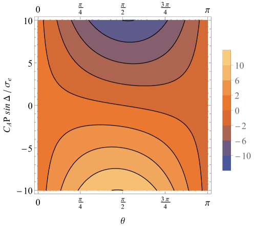
Figure 1: Depiction of $\sigma_{\rm eff.}\cos\theta/\sigma_{e}$. The horizontal axes is the polar angle $\theta$, and the vertical one is $C_{A}P\sin\Delta/\sigma_{e}$. As the figure suggests, for any value of $P$ there exists a range of $\theta$ and $\Delta$ for which $\sigma_{\rm eff.}\cos\theta<0$ and the chiral channel becomes unstable.

As in the nonchiral case, we check the causality of the chiral channel using (3). The leading term for the short wavelength expansion reads

$$\mathcal{D}_{\text{C}}\sim 8ik^{3}v_{g}\left(v_{g}^{2}-1\right)w_{0}\,,$$ (22)

which implies that the chiral channel is causal. The causality of the chiral channel has crucial consequences. First, it implies that the linear stability of the system in a moving frame is similar to the LRF. Second, AH instability is not fictitious. One may be tempted to write a relaxation equation for the current to remove the instability. However, such an approach does not work. Let us remind that the relaxation time approach is essentially employed to avoid instantaneous propagation of signals. The CSMHD modes are, however, causal. Hence a relaxation time approach seems to be useless. We nevertheless use the following ansatz to check whether it can cure the instability problem of this mode

$$\tau_{J}\Delta^{\mu\nu}\mathfrak{D}J_{\nu}+J^{\mu}=\sigma_{e}E^{\mu}\,.$$ (23)

Let us note that since the axionic part of the current is dissipationless, a relaxation equation can only be written for the Ohmic part of the current. An explicit computation of the modes using (23) confirms that the AH instability cannot be removed by this relation.

4 Numerical results

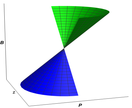
Figure 2: The schematic view of the unstable regions in space. The cone is defined as $\theta=\theta_{c}$, wherein $\theta_{c}$ is the angle at which the effective conductivity (21) vanishes. The upper quarter is the interval $\theta_{c}\leq\theta<\pi/2$ (green), while the lower one is $3\pi/2<\theta\leq\pi-\theta_{c}$ (blue). The chiral channel is unstable within these two quarters and stable outside them.

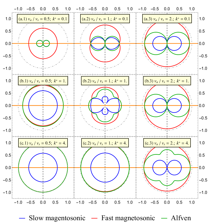
Figure 3: The figures represent the phase velocity $\real(\omega)/k$ in the plane of $\bm{B}_{0}$-$\bm{P}_{0}$. The figures are for different values of $k/\sigma_{e}$ (columns 1, 2, and 3) and $v_{a}/v_{s}$ (rows a, b, and c). For all figures, $P=\sigma_{e}/\left(\sqrt{3}C_{A}\right)$. The horizontal orange gridline in each figure corresponds to the direction of $\bm{B}_{0}$, while the vertical dashed gray gridline is in the direction of $\bm{P}_{0}$. The dash-dotted circle demonstrates the speed of light. The blue and red curves correspond to slow and fast magnetosonic modes in (3.2), respectively. The green curves are the phase velocity of the Alfvén modes in (3.3). The Alfvén modes are symmetric.

Figure 4: The figures represent the phase velocity $\real(\omega)/k$ in the plane perpendicular to $\bm{P}_{0}$. For the upper half-plane, $\Delta=\pi/2$, and in the lower one $\Delta=3\pi/2$. The figures are for different values of $k/\sigma_{e}$ (columns 1, 2, and 3) and $v_{a}/v_{s}$ (rows a, b, and c). For all figures $P=\sigma_{e}/\left(\sqrt{3}C_{A}\right)$. The horizontal orange gridline in each figure corresponds to the direction of $\bm{B}_{0}$, while the vertical dashed gray gridline is in the direction perpendicular to both $\bm{B}_{0}$ and $\bm{P}_{0}$. The dash-dotted circle demonstrates the speed of light. The blue and red curves correspond to slow and fast magnetosonic modes in (3.2), respectively. The green curves are the phase velocity of the Alfvén modes in (3.3). Even for small values of $v_{a}/v_{s}$, the Alfvén modes reach the speed of light in a certain direction.

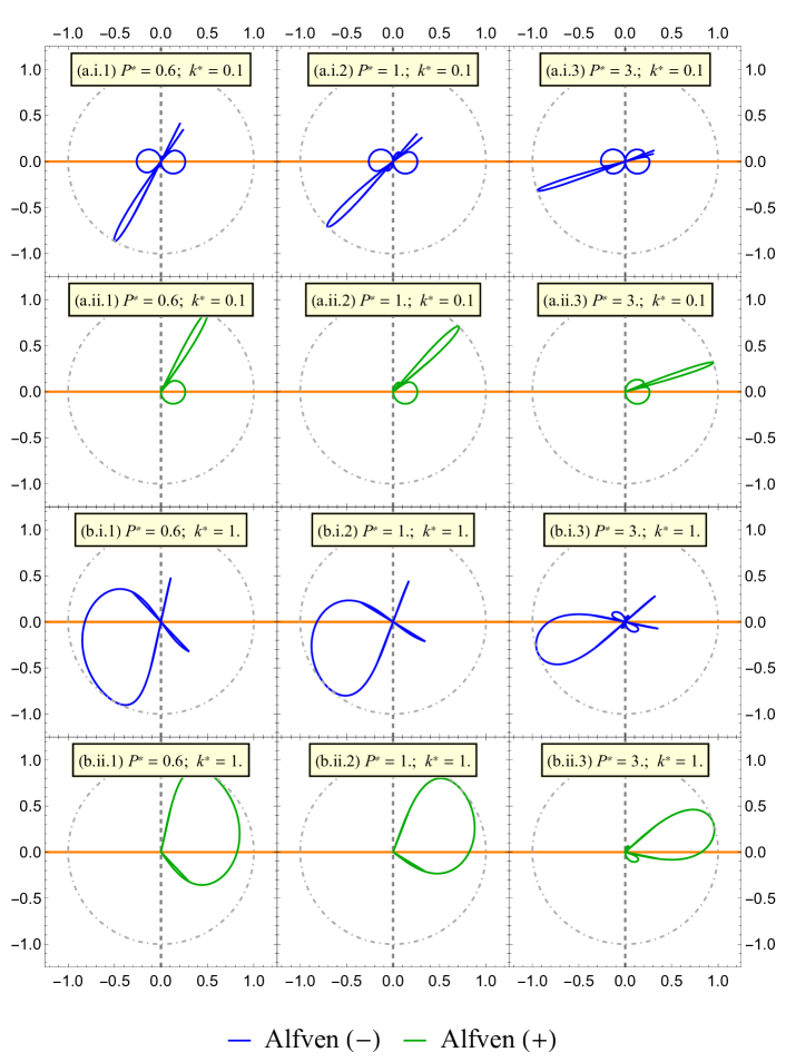
Figure 5: The figures represent the phase velocity $\real(\omega)/k$ of the Alfvén modes in the plane perpendicular to $\bm{P}_{0}$. For the upper half-plane, $\Delta=\pi/2$, and in the lower one $\Delta=3\pi/2$. The figures are for different values of $k/\sigma_{e}$ (columns 1, 2, and 3) and $P^{\star}=C_{A}P/\sigma_{e}$ (rows a and b). Each row is divided into I and ii parts, with i (ii) demonstrating the negative (positive) Alfvén modes of (3.3). $v_{a}/v_{s}=0.5$ for all figures. The horizontal orange gridline in each figure corresponds to the direction of $\bm{B}_{0}$, while the vertical dashed gray gridline is in the direction perpendicular to both $\bm{B}_{0}$ and $\bm{P}_{0}$. The dash-dotted circle demonstrates the speed of light. The positive and negative Alfvén modes propagate with the speed of light in opposite polar directions. This direction gets closer to the direction of $\bm{B}_{0}$ for larger values of $P^{\star}$. The asymmetry decreases for larger values of $k/\sigma_{e}$.

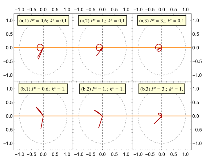
Figure 6: The figures represent the phase velocity $\real(\omega)/k$ of the chiral nonhydro mode in the plane perpendicular to $\bm{P}_{0}$. For the upper half-plane, $\Delta=\pi/2$, and in the lower one $\Delta=3\pi/2$. The figures are for different values of $k/\sigma_{e}$ (columns 1, 2, and 3) and $P^{\star}=C_{A}P/\sigma_{e}$ (rows a and b). For all figures, $v_{a}/v_{s}=0.5$. The horizontal orange gridline in each figure corresponds to the direction of $\bm{B}_{0}$, while the vertical dashed gray gridline is in the direction perpendicular to both $\bm{B}_{0}$ and $\bm{P}_{0}$. The dash-dotted circle demonstrates the speed of light.

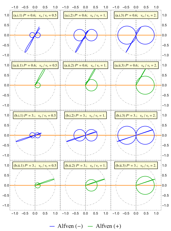
Figure 7: The figures represent the phase velocity $\real(\omega)/k$ of the Alfvén modes in the plane perpendicular to $\bm{P}_{0}$. For the upper half-plane, $\Delta=\pi/2$, and in the lower one $\Delta=3\pi/2$. The figures are for different values of $v_{a}/v_{s}$ (columns 1, 2, and 3) and $P^{\star}=C_{A}P/\sigma_{e}$ (rows a and b). Each row is divided into I and ii parts, with i (ii) demonstrating the negative (positive) Alfvén modes of (3.3). $k/\sigma_{e}=0.1$ for all figures. The horizontal orange gridline in each figure corresponds to the direction of $\bm{B}_{0}$, while the vertical dashed gray gridline is in the direction perpendicular to both $\bm{B}_{0}$ and $\bm{P}_{0}$. The dash-dotted circle demonstrates the speed of light. The positive and negative Alfvén modes propagate with the speed of light in opposite polar directions. This direction gets closer to the direction of $\bm{B}_{0}$ for larger values of $P^{\star}$.

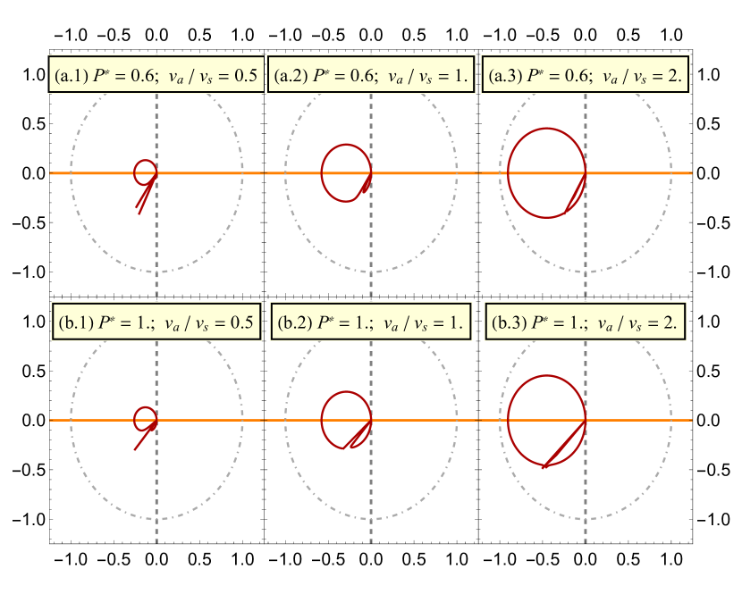
Figure 8: The figures represent the phase velocity $\real(\omega)/k$ of the chiral nonhydro mode in the plane perpendicular to $\bm{P}_{0}$. For the upper half-plane, $\Delta=\pi/2$, and in the lower one $\Delta=3\pi/2$. The figures are for different values of $v_{a}/v_{s}$ (columns 1, 2, and 3) and $P^{\star}=C_{A}P/\sigma_{e}$ (rows a, and b). $k/\sigma_{e}=0.1$ for all figures. The horizontal orange gridline in each figure corresponds to the direction of $\bm{B}_{0}$, while the vertical dashed gray gridline is in the direction perpendicular to both $\bm{B}_{0}$ and $\bm{P}_{0}$. The dash-dotted circle demonstrates the speed of light.

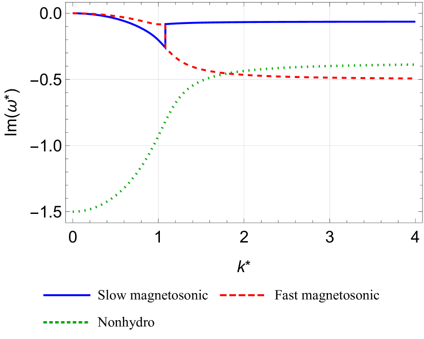
Figure 9: The figure represents $\imaginary(\omega)/\sigma_{e}$ vs. $k/\sigma_{e}$ for the nonchiral channel (10). As shown in the text, $\imaginary(\omega)$ is always negative and the nonchiral channel is stable. The fast magnetosonic modes are suppressed more strongly than the slow ones. $\imaginary(\omega)$ becomes almost constant after a sufficiently large value of $k$.

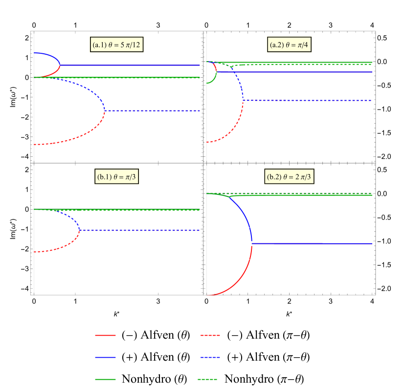
Figure 10: The figure represents $\imaginary(\omega)/\sigma_{e}$ vs. $k/\sigma_{e}$ for the chiral channel (11): (a.1) represents a value of $\theta$ within the upper unstable region of Fig. 2; (a.2) represents a value of $\theta$ within the upper stable region of Fig. 2; (b.1) represents the angle $\theta_{c}$ at which $\sigma_{\rm eff.}=0$ within the upper region of Fig. 2; (b.2) represents the angle $\theta_{c}$ at which $\sigma_{\rm eff.}=0$ within the lower region of Fig. 2. The mode propagating in exactly opposite direction are drawn with the same color but dashed lines. The channel is still stable at this critical angle. The $\imaginary(\omega)$ becomes almost constant after a sufficiently large value of $k^{\star}$.

In this section, we present numerical results for the collective modes. First, we depict the phase velocities $v_{\rm ph}\equiv\real(\omega/k)$ for different modes. We then plot the imaginary part of eigenfrequencies for the nonchiral and chiral channels. Since our results are independent of the electrical conductivity, we make certain quantities dimensionless by dividing them by $\sigma_{e}$

$$\omega^{\star}\equiv\omega/\sigma_{e}\,,\qquad k^{\star}\equiv k/\sigma_{e}\,,\qquad P^{\star}\equiv C_{A}P/\sigma_{e}.$$ (1)

As it turns out, for any particular choice of parameters, there exists two critical polar angles $\theta_{c}$ and $\pi-\theta_{c}$ for which the effective conductivity vanishes

$$\theta_{c}\equiv\arctan(\frac{1}{P^{\star}\sin\Delta})\,.$$ (2)

These angles divide the space into stable and unstable regions. A schematic picture of this division is presented in Fig. 2. The chiral channel is unstable inside the green upper ($\theta_{c}<\theta<\pi/2$) and blue lower ($3\pi/2<\theta<\pi-\theta_{c}$) quarters. The remained symmetries of the space allow us to choose a particular vertical slice, which is the $\bm{B}$-$z$ plane, and a particular horizontal one, which is the $\bm{B}$-$\bm{P}$ plane. In the $\bm{B}$-$z$ plane, $\Delta=\pi/2\leavevmode\nobreak\ (3\pi/2)$ for the upper (lower) half. In the $\bm{B}$-$\bm{P}$ plane $\Delta=0$ for both halves. We note that the absolute value of $\Delta$ is not significant in our analysis, because it can be absorbed into $P^{\star}$, but the sign of $\sin\Delta$ matters. For simplicity, we call the different modes of (3.3) negative Alfvén ($\omega_{\rm A,-}$), positive Alfvén ($\omega_{\rm A,+}$), and chiral nonhydro ($\omega_{\rm C,\rm nh}$) modes.

i) Phase velocities

We use polar plots to depict the phase velocities. To do so, we need to transform from spherical coordinates to polar coordinates in $\bm{B}$-$z$ and $\bm{B}$-$\bm{P}$ planes. In the $\bm{B}$-$z$, we define the polar angle as

$$\varphi\equiv{\rm sgn}\left(\sin\Delta\right)\theta\,.$$

Positive (negative) $\varphi$ corresponds to the upper (lower) half of the $\bm{B}$-$z$ plane. Since $\Delta=0$ for the $\bm{B}$-$\bm{P}$ plane, the upper and lower half-planes are similar. In each figure of Figs. 3-8, the absolute value of the phase velocity at any particular value of $\varphi$ is equal to the radius of the corresponding curve. The sign of the velocity is not shown, and the sign of plot ticks are just indicators of the corresponding quarter. The phase velocities in the $\bm{B}$-$\bm{P}$ plane are depicted in Fig. 3. The modes behave similarly to those of the resistive MHD Kawazura:2017lpc . For small values of $k^{\star}$, the slow magnetosonic and Alfvén modes have similar phase velocities, and the fast magnetosonic modes are the fastest ones. This behavior is not surprising because the limit $k\ll\sigma_{e}$ is the iMHD limit. As $k^{\star}$ increases, the Alfvén modes obtain phase velocities closer to the fast magnetosonic ones. In the nonchiral channel, the phase velocity vanishes for $\cos\theta=0$, as it can be analytically found from (10). On the other hand, a similar general statement cannot be expressed for the phase velocity at $\sin\theta=0$. The special case of $k^{\star}=1$, for which the phase velocity of slow magnetosonic modes becomes equal to the speed of sound, is interesting. The nonhydro mode of the nonchiral channel does not propagate, i.e. its phase velocity is always zero. The modes in the $\bm{B}$-$\bm{P}$ plane are symmetric, and we do not represent any other figure in this plane.

We represent the phase velocities in the $\bm{B}$-$z$ plane with some details. In Fig. 4, the phase velocities of all modes are drawn. In the stable polar region, the phase velocities are similar to those of the $\bm{B}$-$\bm{P}$ plane. However, in the unstable region, the Alfvén modes behave drastically different. Even for small values of $k^{\star}$, there exists a region for which the Alfvén modes propagate with the speed of light. We can understand this behavior by inspecting the first $k$-dependent term in Alfvén phase velocity which is found from (3.3),

$$v_{\rm ph,Alfv\'{e}n}=\pm v_{a}\cos\theta\pm\frac{\left(1-v_{a}^{2}\right)^{2}\left(1-5v_{a}^{2}\cos^{2}\theta\right)\left(1-v_{a}^{2}\cos^{2}\theta\right)}{8v_{a}\cos\theta\sigma_{\rm eff.}^{2}}k^{2}+\order{k^{3}}.$$ (3)

When $\sigma_{\rm eff.}$ becomes very small, the phase velocity increases. But one should keep in mind that the higher order terms are absent in (3), and the phase velocity does not actually tend to infinity as this relation suggests. Also, as (3) suggests, this region widens as $k^{\star}$ increases. For sufficiently large $k^{\star}$, the Alfvén modes obtain the speed of light. In contrast to the magnetosonic modes, the Alfvén ones are asymmetric under the mirror symmetry with respect to the direction of $\bm{B}$: The chiral channel is not symmetric under transformation of $\theta\to\pi-\theta$, while the nonchiral one is. Increasing $v_{a}/v_{s}$, which for a fixed temperature corresponds to stronger magnetic fields, has the same effect as in $\bm{B}$-$\bm{P}$ plane.

In the nonchiral channel, the nonhydro mode has nonzero phase velocity. The negative and positive Alfvén modes overlap with each other and the nonhydro one. Therefore, to better understand the behavior of the chiral channel, we draw the phase velocities separately. The phase velocity of the nonhydro mode cannot be understood using the long-wave expansion (3). However, we can rely on numerical inspection to understand the peculiar behavior of the chiral channel. We start with the chiral channel’s modes in the upper half-plane. In the first stable region, namely $0<\theta<\theta_{c}$, only the Alfvén modes propagate. The phase velocities have opposite signs but equal values. The velocities of these hydro modes are enhanced by increasing $k^{\star}$ (Fig. 5) and $v_{a}/v_{s}$ (Fig. 7). The velocities tend to the speed of light as we get closer to the critical angle. At the critical angle, the negative Alfvén mode is replaced by the nonhydro one. Both modes propagate with the speed of light. For the nonhydro mode, this only happens exactly at the critical angle and is not captured in Fig. Fig. 6. Then we enter the upper unstable region, i.e. $\theta_{c}<\theta<\pi/2$. In this region, there is a subregion for which the modes propagate. The subregion widens in larger values of $k^{\star}$. For small values of $k^{\star}$, the negative Alfvén mode obtain positive velocities, while the positive Alfvén mode is replaced by the nonhydro mode, which has a negative velocity. As $k^{\star}$ is increased, the nonhydro mode is suppressed, and the positive and negative Alfvén modes obtain velocities with the right signs. The same remarks hold for the second quarter of the upper half-plane. The modes behave similarly in the lower half-planes, with negative and positive Alfvén modes swapped.

ii) Imaginary parts

In Figs. 9 and 10 the $k^{\star}$ dependence of the imaginary parts of all modes in both channels are plotted. As it turns out, they become almost constant after a particular value of $k^{\star}$. In particular, the imaginary parts of the nonchiral channel modes, presented in Fig. 9, are always negative. This confirms our proof presented in Appendix B. For the chiral channel, the imaginary parts become positive in the unstable regions. Let us also notice that in Fig. 10 the modes in the exact opposite direction have negative imaginary parts. The imaginary parts of the modes at the two critical angles are also depicted in Fig. 10. All imaginary parts vanish in the direction of the critical angle, while in the exact opposite direction they have nonvanishing negative values. Therefore at the critical angle, the chiral channel is still stable.

5 Concluding remarks

In the present work, we performed an analysis of the linear stability of a resistive CSMHD. We started with the MCS Lagrangian that produces the CM current through the comoving temporal derivative of an axion-like field. After reproducing the results of Ozonder:2010zy for the MCS thermodynamics, we identified the global equilibrium state in CSMHD by applying a standard entropy current analysis. We showed that the axial chemical potential $\mu_{5}$ vanishes in global equilibrium, but the spatial gradient of the axion $\bm{P}=\gradient{\mathrm{\Theta}}$ can give rise to a nonzero electrical charge density. To proceed, we chose the conjugate chemical potential of the electrical charge density $\mu_{e}$ to be zero in the equilibrium. This choice is equivalent to the power counting scheme in which the magnetic field is of order $\order{1}$, while the electric field is of order $\order{\partial}$. Hence, in this weak electric field regime Hernandez:2017mch , the electric field vanishes in the thermodynamical equilibrium. As a consequence, the electric charge density vanishes, and the spatial gradient of the axion-like field is constrained to be perpendicular to the magnetic field. With the hydrostatic configuration fixed, we introduced linear perturbation to find the collective modes. We found that there exist three extra modes in CSMHD, in addition to the six ones of iMHD. These nine modes are divided into two channels: Five in a nonchiral or non-axionic channel and four in a chiral or axionic one. The nonchiral channel consists of slow and fast magnetosonic modes, which are damped by the nonzero electrical resistivity. This channel also possesses a nonhydro (gapped) mode. Using the Routh-Hurwitz criteria and asymptotic causality condition, we showed that the nonchiral channel is linearly stable and causal. The chiral channel includes the modified Alfvén modes and a nonhydro (gapless) mode. The stability of these modes is controlled by a combination of the Ohm and AH conductivities, which can be considered as a novel effective conductivity. In contrast to the Ohm conductivity, effective conductivity becomes negative for the modes propagating sufficiently close to the direction of the magnetic field. Consequently, the chiral channel is unstable in this region. However, this channel is causal, and therefore the instability is physical. We also performed a numerical inspection of phase velocities and imaginary parts of different modes. As our results show, there is a critical angle that separates stable and unstable regions of the space for the chiral channel. In the direction of this critical angle, the Alfvén waves travel with the speed of light without becoming unstable.

The current work has a theoretical nature, in which we explored the stability and causality of the modes propagating in a chiral medium. Although the CM current that arises from the MCS theory has a physical explanation, this theory is not the only approach to the CME. To the best of our knowledge, other consequences of the MCS theory are not well understood in the context of the QGP physics. In particular, in contrast to the condensed matter physics Liu2016 , we are unaware of a physical explanation for the occurrence of the AH effect in the QGP. It might be interesting to investigate the possible mechanisms that give rise to the AH effect in different states of strongly interacting quark matter.

We close this paper by suggesting two possible directions that extend this work. In the present work, we have assumed that the electric chemical potential is zero, which is equivalent to the assumption of electric field being of order $\order{\partial}$. A possible extension would be to consider the strong electric field regime, in which the electric field is of order $\order{1}$ and the electric chemical potential is nonzero in the equilibrium. Another interesting extension is to assume the equilibrium state to be in a rigid rotation. The work in both directions is in progress.

Appendix A Notations, conventions and useful formulae

The energy-momentum tensor of the perfect fluid is given by Landau1987Fluid ; rezzolla ; Kovtun:2012rj

$$T^{\mu\nu}_{\text{Fluid}(0)}=\varepsilon u^{\mu}u^{\nu}-p\Delta^{\mu\nu}.$$ (1)

Here, $\varepsilon$ is the energy density, $p$ the pressure, and $u^{\mu}$ the fluid four-velocity normalized as $u^{\mu}u_{\mu}=1$. These so-called hydrodynamic variables have unique definitions for the perfect fluid Kovtun:2012rj . Consequently, the LRF is unambiguously defined by $u^{\mu}=(1,\bm{0})$. In (1), $\Delta_{\mu\nu}\equiv g_{\mu\nu}-u_{\mu}u_{\nu}$ projects vectors and tensors in the direction orthogonal to $u_{\mu}$. The comoving temporal $\mathfrak{D}$ and spatial derivatives $\nabla^{\bot}_{\mu}{}$ read

$$\mathfrak{D}\equiv u^{\mu}\partial_{\mu},\qquad\nabla^{\bot}_{\mu}{}\equiv\Delta^{\nu}_{\mu}\partial_{\nu}.$$ (2)

As any antisymmetric tensor of rank two, $F_{\mu\nu}$ and ${{}^{\star}{F}}_{\mu\nu}$ can be decomposed with respect to the timelike vector $u_{\mu}$ Bekenstein1978

$$F_{\mu\nu}=E_{\mu}u_{\nu}-E_{\nu}u_{\mu}-\epsilon_{\mu\nu\alpha\beta}B^{\alpha}u^{\beta},\qquad{{}^{\star}{F}}_{\mu\nu}=B_{\mu}u_{\nu}-B_{\nu}u_{\mu}+\epsilon_{\mu\nu\alpha\beta}E^{\alpha}u^{\beta},$$ (3)

where the EM four-vectors are defined as

$$E^{\mu}\equiv F^{\mu\nu}u_{\nu},\qquad B^{\mu}\equiv\frac{1}{2}\epsilon^{\mu\nu\alpha\beta}F_{\nu\alpha}u_{\beta}.$$ (4)

One should bear in mind that only for the comoving observer, say in the LRF, the above four-vectors coincide with the physical electric and magnetic fields, i.e. $E^{\mu}=(0,\bm{E})$ and $B^{\mu}=(0,\bm{B})$. By this virtue

$$E\equiv\sqrt{-E^{\mu}E_{\mu}}=\absolutevalue*{\bm{E}}_{\text{LRF}},\mbox{\quad and\quad}B\equiv\sqrt{-B^{\mu}B_{\mu}}=\absolutevalue*{\bm{B}}_{\text{LRF}}.$$ (5)

We note that while $E$ and $B$ are Lorentz invariants, $\absolutevalue*{\bm{E}}$ and $\absolutevalue*{\bm{B}}$ are not.

Appendix B Routh-Hurwitz stability analysis

In this appendix, we apply the Routh-Hurwitz stability criteria Krotscheck1978 to channels found in Sec. 3.

B.1 Nonchiral channel

For simplicity, we rewrite the nonchiral channel (10) as

$$\mathcal{D}_{\text{NC}}^{\prime} \equiv \frac{1-v_{a}^{2}}{w_{0}}\mathcal{D}_{\text{NC}}=\sigma_{e}v_{a}^{2}(\omega^{2}-k^{2})\left(2\omega^{2}-v_{s}^{2}k^{2}\right)-2\omega(1-v_{a}^{2})\left(\omega^{2}-v_{s}^{2}k^{2}\right)\left(ik^{2}+\omega(\sigma_{e}-i\omega)\right)$$ (1)

$$-v_{s}^{2}k^{2}n_{e}v_{a}^{2}\cos(2\theta)\left(\omega^{2}-k^{2}\right).$$

To apply the Routh-Hurwitz criteria, we perform the substitution $\omega\rightarrow i\zeta$ Kovtun:2019hdm . Consequently, $\mathcal{D}_{\text{NC}}^{\prime}$ is transformed into a $5$th order polynomial in $\zeta$,

$$\mathcal{D}_{\text{NC}}^{\prime}=\sum_{i=0}^{5}a_{i}\zeta^{i}\,.$$

We employ, at this stage, the Routh-Hurwitz criteria to find whether the real part of $\zeta$ is positive. The Routh table reads

$${\rm R}_{\rm NC}=\left(\begin{array}[]{ccc}a_{5}&a_{3}&a_{1}\\ a_{4}&a_{2}&a_{0}\\ b_{1}&b_{2}&0\\ c_{1}&c_{2}=a_{0}&0\\ d_{1}&0&0\\ e_{1}=a_{0}&0&0\\ \end{array}\right).$$ (2)

The coefficients $a_{i}$ read

$$a_{0} = 2v_{s}^{2}k^{4}\sigma_{e}v_{a}^{2}\cos^{2}\theta\,,\qquad a_{1}=2v_{s}^{2}(1-v_{a}^{2})k^{4}\,,\qquad a_{2}=2k^{2}\sigma_{e}\left[v_{s}^{2}+v_{a}^{2}\left(1-v_{s}^{2}\sin^{2}\theta\right)\right]\,,$$

$$a_{3} = 2\left(1+v_{s}^{2}\right)\left(1-v_{a}^{2}\right)k^{2}\,,\qquad a_{4}=2\sigma_{e}\,,\qquad a_{5}=2\left(1-v_{a}^{2}\right).$$

All of the above coefficients are positive. Therefore, according to the criteria, all other elements in the first column of the Routh table (2) must also be positive to ensure $\real(\zeta)>0$. The next two coefficients are

$$b_{1} = \frac{a_{3}a_{4}-a_{2}a_{5}}{a_{4}}=2k^{2}\left(1-v_{a}^{2}\right)\left(1-v_{a}^{2}+v_{a}^{2}v_{s}^{2}\sin^{2}\theta\right)\,,$$

$$b_{2} = \frac{a_{4}a_{1}-a_{0}a_{5}}{a_{4}}=2k^{4}v_{s}^{2}\left(1-v_{a}^{2}\right)\left(1-v_{a}^{2}\cos^{2}\theta\right).$$

The positivity of the above coefficients is obvious. We now turn to $c_{1}$,

$$c_{1} = \frac{a_{2}b_{1}-a_{4}b_{2}}{b_{1}}=\frac{2k^{2}\sigma_{e}}{1-v_{a}^{2}+v_{s}^{2}v_{a}^{2}\sin^{2}\theta}\Bigg{[}\left(1-v_{a}^{2}\right)\left(1-2v_{s}^{2}\sin^{2}\theta\right)$$ (3)

$$\hskip 85.35826pt+v_{s}^{4}\sin^{2}\theta\left(1-v_{a}^{2}\sin^{2}\theta\right)\Bigg{]}\,.$$

The positivity of the terms outside the brackets is apparent. The expression inside the bracket can be assumed as a second-order polynomial in $v_{s}^{2}$, whose discriminant is negative

$$\Delta=-(1-v_{a}^{2})\sin[2](2\theta)<0\,.$$

Since $(1-v_{a}^{2})>0$, $c_{1}$ is also positive. By the same virtue, $d_{1}$ is positive

$$d_{1} = \frac{b_{2}c_{1}-b_{1}c_{2}}{c_{1}}=\frac{b_{2}c_{1}-b_{1}a_{0}}{c_{1}}=2v_{s}^{2}\left(1-v_{s}^{2}\right)^{2}\left(1-v_{a}^{2}\right)^{2}k^{4}\cos[4](\theta)\Bigg{[}\left(1-v_{a}^{2}\right)\left(1-2v_{s}^{2}\sin^{2}\theta\right)$$ (4)

$$\hskip 113.81102pt+v_{s}^{4}\sin^{2}\theta\left(1-v_{a}^{2}\sin^{2}\theta\right)\Bigg{]}^{-1}>0\,.$$

We conclude that all elements of the first column of the Routh table (2) have the same sign. The nonchiral channel is thus stable.

B.2 Chiral channel

As for the nonchiral case, we rewrite the chiral channel as

$$\mathcal{D}_{\text{C}}^{\prime}=\frac{1-v_{a}^{2}}{8w_{0}} = -\sigma_{\rm eff.}\cos\theta\left(\omega^{2}-k^{2}v_{a}^{2}\cos^{2}\theta\right)+i\omega\cos\theta\left(1-v_{a}^{2}\right)\left(\omega^{2}-k^{2}\right).$$ (5)

Performing substitution $\omega\rightarrow i\zeta$ gives rise to a third order polynomial in $\zeta$

$$\mathcal{D}_{\text{C}}^{\prime}=\sum_{i=0}^{3}a_{c,i}\zeta^{i}\,,$$

The coefficients read

$$a_{c,0}=k^{2}v_{a}^{2}\sigma_{\rm eff.}\cos^{3}\theta\,,\quad a_{c,1}=k^{2}\left(1-v_{a}^{2}\right)\cos\theta\,,\quad a_{c,2}=\sigma_{\rm eff.}\cos\theta\,,\quad a_{c,3}=\left(1-v_{a}^{2}\right)\cos\theta\,.$$ (6)

We do not need to reproduce the whole Routh table to realize that the chiral channel is unstable for regions of $\theta$. For the coefficients to have the same sign, it is required that

$$\sigma_{\rm eff.}\cos\theta>0\,.$$

As stated in Sec. 3, such a condition cannot be satisfied for all values of $\theta$. This is visualized in Fig. 1. We conclude that the modes of the chiral channel are always unstable within a region around the direction transverse to the magnetic field.

- (1) L.D. Landau and E.M. Lifshitz, Fluid Mechanics, Butterworth-Heinemann, 2 ed. (Jan., 1987).
- (2) L. Rezzolla and O. Zanotti, Relativistic Hydrodynamics, OUP Oxford (2013).
- (3) B. Schenke, S. Jeon and C. Gale, (3+1)d hydrodynamic simulation of relativistic heavy-ion collisions, Phys. Rev. C 82 (2010) 014903 [1004.1408].
- (4) B. Schenke, S. Jeon and C. Gale, Elliptic and triangular flow in event-by-event (3+1)d viscous hydrodynamics, Phys. Rev. Lett. 106 (2011) 042301 [1009.3244].
- (5) J.-F. Paquet, C. Shen, G.S. Denicol, M. Luzum, B. Schenke, S. Jeon et al., Production of photons in relativistic heavy-ion collisions, Phys. Rev. C 93 (2016) 044906 [1509.06738].
- (6) W. Florkowski, M.P. Heller and M. Spalinski, New theories of relativistic hydrodynamics in the LHC era, Rept. Prog. Phys. 81 (2018) 046001 [1707.02282].
- (7) W. Hiscock and L. Lindblom, Stability and causality in dissipative relativistic fluids, Annals Phys. 151 (1983) 466.
- (8) W.A. Hiscock and L. Lindblom, Generic instabilities in first-order dissipative relativistic fluid theories, Phys. Rev. D 31 (1985) 725.
- (9) P. Kovtun, First-order relativistic hydrodynamics is stable, JHEP 10 (2019) 034 [1907.08191].
- (10) P. Romatschke, Do nuclear collisions create a locally equilibrated quark–gluon plasma?, Eur. Phys. J. C 77 (2017) 21 [1609.02820].
- (11) M.P. Heller and M. Spalinski, Hydrodynamics beyond the gradient expansion: Resurgence and resummation, Phys. Rev. Lett. 115 (2015) 072501 [1503.07514].
- (12) P. Kovtun, Lectures on hydrodynamic fluctuations in relativistic theories, J. Phys. A 45 (2012) 473001 [1205.5040].
- (13) J.D. Bekenstein and E. Oron, New conservation laws in general-relativistic magnetohydrodynamics, Phys. Rev. D 18 (1978) 1809.
- (14) X.-G. Huang, Electromagnetic fields and anomalous transports in heavy-ion collisions — A pedagogical review, Rept. Prog. Phys. 79 (2016) 076302 [1509.04073].
- (15) G.S. Denicol, E. Molnár, H. Niemi and D.H. Rischke, Resistive dissipative magnetohydrodynamics from the Boltzmann-Vlasov equation, Phys. Rev. D 99 (2019) 056017 [1902.01699].
- (16) G.M. Newman, Anomalous hydrodynamics, JHEP 01 (2006) 158 [hep-ph/0511236].
- (17) D.T. Son and P. Surowka, Hydrodynamics with triangle anomalies, Phys. Rev. Lett. 103 (2009) 191601 [0906.5044].
- (18) W. Florkowski, B. Friman, A. Jaiswal and E. Speranza, Relativistic fluid dynamics with spin, Phys. Rev. C 97 (2018) 041901 [1705.00587].
- (19) N. Sadooghi and S.M.A. Tabatabaee, The effect of magnetization and electric polarization on the anomalous transport coefficients of a chiral fluid, New J. Phys. 19 (2017) 053014 [1612.02212].
- (20) D.E. Kharzeev, L.D. McLerran and H.J. Warringa, The effects of topological charge change in heavy ion collisions: ’Event by event P and CP violation’, Nucl. Phys. A 803 (2008) 227 [0711.0950].
- (21) K. Fukushima, D.E. Kharzeev and H.J. Warringa, The chiral magnetic effect, Phys. Rev. D 78 (2008) 074033 [0808.3382].
- (22) K. Hattori, Y. Hirono, H.-U. Yee and Y. Yin, MagnetoHydrodynamics with chiral anomaly: Phases of collective excitations and instabilities, Phys. Rev. D 100 (2019) 065023 [1711.08450].
- (23) A. Boyarsky, J. Fröhlich and O. Ruchayskiy, Magnetohydrodynamics of chiral relativistic fluids, Phys. Rev. D 92 (2015) 043004.
- (24) I. Rogachevskii, O. Ruchayskiy, A. Boyarsky, J. Fröhlich, N. Kleeorin, A. Brandenburg et al., Laminar and turbulent dynamos in chiral magnetohydrodynamics-I: Theory, Astrophys. J. 846 (2017) 153 [1705.00378].
- (25) I. Shovkovy, D. Rybalka and E. Gorbar, The overdamped chiral magnetic wave, PoS Confinement2018 (2018) 029 [1811.10635].
- (26) N. Sadooghi and M. Shokri, Rotating solutions of nonideal transverse Chern-Simons magnetohydrodynamics, Phys. Rev. D 98 (2018) 076011 [1806.06652].
- (27) D.E. Kharzeev, Topologically induced local P and CP violation in QCD QED, Annals Phys. 325 (2010) 205 [0911.3715].
- (28) E. Witten, Dyons of Charge e theta/2 pi, Phys. Lett. B 86 (1979) 283.
- (29) F. Wilczek, Two applications of axion electrodynamics, Phys. Rev. Lett. 58 (1987) 1799.
- (30) S.M. Carroll, G.B. Field and R. Jackiw, Limits on a Lorentz and parity violating modification of electrodynamics, Phys. Rev. D 41 (1990) 1231.
- (31) K. Landsteiner, Notes on anomaly induced transport, Acta Phys. Polon. B 47 (2016) 2617 [1610.04413].
- (32) S. Ozonder, Maxwell-Chern-Simons hydrodynamics for the chiral magnetic effect, Phys. Rev. C 81 (2010) 062201 [1004.3883].
- (33) S. Ozonder, Erratum: Maxwell-chern-simons hydrodynamics for the chiral magnetic effect [phys. rev. c 81, 062201(r) (2010)], Phys. Rev. C 84 (2011) 019903.
- (34) P. Kovtun, Thermodynamics of polarized relativistic matter, JHEP 07 (2016) 028 [1606.01226].
- (35) J. Hernandez and P. Kovtun, Relativistic magnetohydrodynamics, JHEP 05 (2017) 001 [1703.08757].
- (36) M. Gedalin, Linear waves in relativistic anisotropic magnetohydrodynamics, Phys. Rev. E 47 (1993) 4354.
- (37) J.D. Bekenstein and G. Betschart, Perfect magnetohydrodynamics as a field theory, Phys. Rev. D 74 (2006) 083009 [gr-qc/0608053].
- (38) C. Aguiar, E. Fraga and T. Kodama, Hydrodynamical instabilities beyond the chiral critical point, J. Phys. G 32 (2006) 179 [nucl-th/0306041].
- (39) J.L. Friedman and N. Stergioulas, Rotating Relativistic Stars, Cambridge Monographs on Mathematical Physics, Cambridge University Press (3, 2013), 10.1017/CBO9780511977596.
- (40) K. Jensen, R. Loganayagam and A. Yarom, Anomaly inflow and thermal equilibrium, 1310.7024 [hep-th].
- (41) J. Kapusta and C. Gale, Finite-temperature Field Theory: Principles and Applications, Cambridge Monographs on Mathematical Physics, Cambridge University Press (2011), 10.1017/CBO9780511535130.
- (42) W. Israel, Nonstationary irreversible thermodynamics: A Causal relativistic theory, Annals Phys. 100 (1976) 310.
- (43) F. Becattini, Covariant statistical mechanics and the stress-energy tensor, Phys. Rev. Lett. 108 (2012) 244502 [1201.5278].
- (44) A. Zee, Einstein Gravity in a Nutshell, Princeton University Press, New Jersey (5, 2013).
- (45) S. De Groot, Relativistic Kinetic Theory. Principles and Applications (1, 1980).
- (46) S. Pu, T. Koide and D.H. Rischke, Does stability of relativistic dissipative fluid dynamics imply causality?, Phys. Rev. D 81 (2010) 114039 [0907.3906].
- (47) E.J. Routh, A treatise on the stability of a given state of motion: Particularly steady motion, Macmillan (1877).
- (48) A. Hurwitz, Ueber die bedingungen, unter welchen eine gleichung nur wurzeln mit negativen reellen theilen besitzt, Mathematische Annalen 46 (1895) 273.
- (49) E. Krotscheck and W. Kundt, Causality criteria, Communications in Mathematical Physics 60 (1978) 171.
- (50) P. Pesic, Abel’s proof. An essay on the sources and meaning of mathematical unsolvability. Reprint, Cambridge, MA: MIT Press (2004).
- (51) Y. Kawazura, Modification of magnetohydrodynamic waves by the relativistic Hall effect, Phys. Rev. E 96 (2017) 013207 [1706.07077].
- (52) C.-X. Liu, S.-C. Zhang and X.-L. Qi, The quantum anomalous hall effect: Theory and experiment, Annual Review of Condensed Matter Physics 7 (2016) 301 [https://doi.org/10.1146/annurev-conmatphys-031115-011417].