A System for 3D Reconstruction Of Comminuted Tibial Plafond Bone Fractures

Abstract

High energy impacts at joint locations often generate highly fragmented, or comminuted, bone fractures. Current approaches for treatment require physicians to decide how to classify the fracture within a hierarchy fracture severity categories. Each category then provides a best-practice treatment scenario to obtain the best possible prognosis for the patient. This article identifies shortcomings associated with qualitative-only evaluation of fracture severity and provides new quantitative metrics that serve to address these shortcomings. We propose a system to semi-automatically extract quantitative metrics that are major indicators of fracture severity. These include: (i) fracture surface area, i.e., how much surface area was generated when the bone broke apart, and (ii) dispersion, i.e., how far the fragments have rotated and translated from their original anatomic positions. This article describes new computational tools to extract these metrics by computationally reconstructing 3D bone anatomy from CT images with a focus on tibial plafond fracture cases where difficult qualitative fracture severity cases are more prevalent. Reconstruction is accomplished within a single system that integrates several novel algorithms that identify, extract and piece-together fractured fragments in a virtual environment. Doing so provides objective quantitative measures for these fracture severity indicators. The availability of such measures provides new tools for fracture severity assessment which may lead to improved fracture treatment. This paper describes the system, the underlying algorithms and the metrics of the reconstruction results by quantitatively analyzing six clinical tibial plafond fracture cases.

1 Introduction

Accurate reconstruction of a patient’s original bone anatomy is the desired outcome for surgical treatment of a bone fracture. Treatment goals include achieving expeditious reconstruction and avoiding Post-Traumatic OsteoArthritis (PTOA). When there is involvement of an articulating joint such as the hip, knee, or ankle, accurate reconstruction of the bone joint surface is critical to avoid PTOA. This task can be quite challenging when dealing with highly comminuted fractures. This is due to the fact that often dozens of individual fragments are involved and they are sometimes displaced significantly from their original anatomic position and scattered in a complex geometric pattern.

This article describes a system for 3D medical image and surface analysis that enables vital new orthopaedic research to improve treatment for traumatic limb bone fractures. An emphasis is placed on the tibial plafond fracture as it is both difficult to treat and can exhibit wide disparity in subjective fracture severity evaluation. This article details a system constructed as a novel integration of algorithms that jointly enable virtual 3D reconstruction of a comminuted bone fracture from a 3D CT image of the fractured limb. While the reconstruction result could be used for pre-operative planning, this article describes the application of this system for the purpose of extracting quantitative data for fracture severity classification.

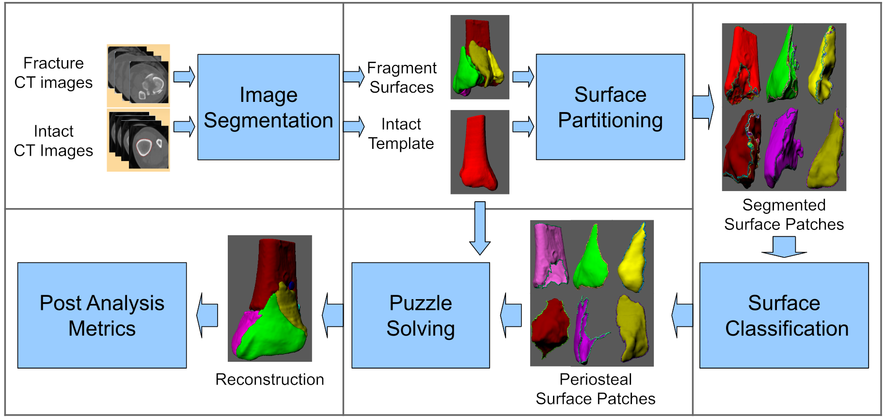
Figure 1: A brief overview of a system proposed in this paper. This system takes as input a 3D CT image of the fractured limb and a 3D CT image of the undamaged (intact) limb, and provides as output a virtual reconstruction of bone fragments which estimates the anatomy of the patient’s original bone. Each block denotes a step and the associated algorithm name is shown inside the block (in blue). Images show how the data has been changed in each step of the 5-step reconstruction process.

Accurately classifying the severity of highly comminuted bone fractures can be challenging for orthopedic physicians and surgeons. Research in (Marsh et al., 2002; Beardsley et al., 2005; Anderson et al., 2008b) states that accurate determination of the initial fracture severity as afforded by fracture severity classification is the single most important prognostic determinant of long-term joint health subsequent to trauma. Due to the importance of fracture severity classification, many researchers (Charalambous et al., 2007; Brumback and Jones, 1994; Thomas et al., 2007; Anderson et al., 2008a; Beardsley et al., 2005) have investigated this problem where their common goal is to define methods capable of predicting fracture severity from quantitative measurements derived from medical image data. Yet, no approach to date provides a holistic solution to this difficult problem as an integrated system.

Our system accomplishes this task as a sequence of three steps:

1. Fragment surfaces are extracted from CT images,

2. Each fragment surface is further decomposed into anatomically meaningful sub-regions,

3. Fragments are pieced back together in a virtual space with a puzzle-solving algorithm.

Quantitative data is extracted for fracture severity assessment is recovered as a by-product of the puzzle-solving solution. The system enables extraction of previously unavailable quantitative information from fractures cases in terms of the bone fragment data to assist physicians in determining the clinical fracture severity classification of comminuted bone fractures.

Results focus on application of this technology to tibial plafond fractures. These fractures typically occur as a result of high-energy trauma such as a ballistic penetration, vehicular accident, or falls from a height. This article focuses on tibial plafond fracture cases for the following reasons:

1. The complex characteristics of this kind of fracture can often create difficulties for physicians in making accurate and reliable fracture severity assessments,

2. Tibia fractures often involve the ankle joint which is typically difficult to treat,

3. The quality of reconstruction is a critical factor for good prognosis,

4. PTOA is directly related to the accuracy of reconstruction.

Hence, this sub-domain of fractures represents one of the most promising applications of the research described herein.

2 Related Work

Computational puzzle solving in 3D seeks to use computer algorithms to facilitate reconstructing 3D broken objects from the geometry of their fragments. In general, puzzle-solving approaches fall into three categories: (1) boundary matching, i.e., algorithms that match together fragments by comparing their boundaries, (2) template matching, i.e., algorithms that match fragments into an a-priori known template that is used as a reference shape for the broken fragments and (3) manual reconstruction approaches. Approaches from the first two categories require algorithms for curve and surface matching and surface alignment. For boundary matching, boundary curves from the broken fragments are matched to piece together the fragments. For template matching, surfaces on the fragment are matched to the corresponding surfaces on the template so that fragments can be aligned into the template to accomplish reconstruction.

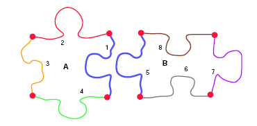
(a)

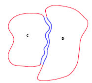
(b)

Figure 2: The difference between reassembling (a) commercial jigsaw puzzles and reconstructing (b) broken artifacts. Note here that the latter is made much more difficult as corners are not easily identifiable and may not indicate the beginning or end of a curve that will uniquely match some other fragment. Worse, any portion of a boundary curve may match to any other fragment and the curve itself may match equally well with numerous similar boundaries from other fragments. (Used with permission from Willis and Cooper (2008). )

Boundary matching approaches for puzzle solving starts with seminal work (Freeman H, 1964; Wolfson et al., 1988) that developed algorithms to piece together 2D jigsaw puzzles similar to that depicted in figure 2. However, solving 3D bone fracture “puzzles” is a significantly more challenging problem. Jigsaw pieces share similar sizes and have distinctly identifiable shapes that greatly restrict the collection of potential mating surfaces/curves on corresponding pieces. Further, for jigsaw puzzles one can assume that all of the jigsaw pieces are complete and intact, and no pieces are missing. Puzzle-solving 3D fractures includes low-resolution sensed data (segmented CT), deformable fragments (bone tissue), potentially nondescript fracture surfaces (similar to oblique planes) and due to a high-energy impact there may be small, missing or unusable fracture pieces.

Fracture reconstruction from boundary data matches boundaries and surfaces generated due to the fracture event. Some work on bone fragment reconstruction uses simulated data by simulating fractures via computer-generated fractures or by using a drop-tower to break bone surrogate material. Examples include (Kronman and Joskowicz, 2013) which simulates a fracture by slicing the intact CT scan of a healthy bone. This allows quick experimentation on a variety of test cases. However, these simulations do not capture the complex physiological or biomechanical phenomena that give rise to these fractures which tend to create fractures that may never been seen in clinical practice. Further, the approach analyzes the geometry of the fracture surface generated by separating bone fragments and assumes these surfaces will accurately fit together using some fracture surface matching metric when in reality bone fragment fracture surfaces may not geometrically match well. In (Willis et al., 2007) tibial plafond fractures are simulated using a drop tower to simulate high axial load to the ankle joint to fracture surrogate bone constructed from high-density polyether urethane foam. Resulting fragments were subsequently scanned in a laboratory setting an fracture surfaces were matched to puzzle-solve the fracture. Here, the measured data and extracted surfaces exhibit little noise which makes reconstruction much easier. Work in (Fürnstahl et al., 2012) proposes an approach for reconstructing proximal humerous joint by alignment of fracture surfaces. A concern here is the geometric accuracy of extracted fracture surface segmentation; especially in low-contrast trebecular bone tissue regions. We opt to align outer bone surfaces only avoiding the potentially inaccurate measurements of the fracture surface regions.

A second category of approaches for bone fragment reconstruction focuses on aligning fragments into a template of the intact bone. Alignment is often achieved through applications of the Iterative Closest Point (ICP) algorithm. This has the distinct disadvantage that, especially in cases where fragments have undergone large displacements or rotations, the ICP algorithm can converge on local minima, giving inaccurate results. In (Chowdhury et al., 2009), work is done on reconstructing facial fractures. As the geometry here is more unique than the tibia, the assumption can be made that each bone surface will have only one match. Because of the differences between comminuted tibia fractures and craniofacial fractures, the effectiveness of ICP in this context translates poorly to our application. The work done in (Albrecht and Vetter, 2012) demonstrates that, with modification, the ICP algorithm can improve upon current reconstruction standards. While a deliberate effort is made to lessen the likelihood of an erroneous convergence of the algorithm, it is still possible and is thus an undesirable algorithm. Other work in (Okada et al., 2009) reconstructs fragments of the proximal femur for fracture cases involving up to 4 fragments by matching fragment outer surfaces and their boundaries. While multiple fragment solutions are described, there are examples of a multi-fragment solution and no computational framework to cope with the large number of potential matches between fragments, fragment boundaries and their unknown potential locations. (Moghari and Abolmaesumi, 2008) defines an Euclidean invariant coordinate system within which to fit algebraic, i.e., implicit polynomial, surface representations to bone fragments surfaces and uses the coefficients of the polynomial models to identify matches between fragments and their corresponding atlas locations.

Several bone fragment reconstruction methods have been documented that are dependent on manual input. In (Scheuering et al., 2001), a system is proposed that simulates volumetric collision detection in a virtual 3D environment and an optimization process for repositioning the bone fragments. In this application, users manually place the fragments close together, then refine the alignment via computer optimization. This method is made more interactive by the work in (Harders et al., 2007), which takes a similar approach of user-guided reconstruction with collision detection while adding haptic feedback to the system. This more advanced human-computer interaction increases the intuitiveness of the system for users. Work in (Cimerman and Kristan, 2007; Kovler et al., 2015) proposes user-guided reconstruction with collision detection while adding surgery simulation. These reconstruction approaches all focus on manual, i.e., interactive alignment, whose applications include pre-operative planning, virtual surgical procedures or surgical training. In contrast, this work targets objective extraction of fracture metrics for severity analysis. As such, we seek to minimize interaction which can bias computed results.

This work represents a significant advancement in fracture reconstruction state-of-the-art in several important ways:

1. it demonstrates reconstruction solutions for clinical data which include the most comminuted, i.e., complex, fracture cases in the literature to date (10 fragments).

2. it incorporates computational acceleration methods required by complex cases which significantly reduce computational cost.

3. it exhibits smaller average reconstruction alignment errors than observed in competing solutions (Okada et al., 2009; Moghari and Abolmaesumi, 2008; Fürnstahl et al., 2012).

Further, the end-purpose of the system as a means to facilitate fracture severity assessment is novel relative to other implementations which focus on surgical planning.

3 Methods

Input: Two 3D CT images: (1) a fractured limb CT, $\mathbf{I}_{f}(x,y,z)$, and (2) an intact (contralateral) limb CT$,\mathbf{I}_{i}(x,y,z)$.

Output: The reduced fracture poses, $\mathbf{T}_{k}$, and fracture severity analysis data, ${\cal A}_{k}$.

 

1: ${\cal S}^{T}={\cal F}\left\{\mathbf{I}_{i}\right\}$: The template bone surface ${\cal S}^{T}$ is extracted from the intact CT image $\mathbf{I}_{i}$. ${\cal{O}}(N^{3})$

2: ${\cal D}_{j}^{T}={\cal E}\left\{{\cal S}^{T}\right\}$: Surface descriptors, ${\cal D}_{j}^{T}$, are extracted from the template bone surface, ${\cal S}^{T}$.

3: ${\cal S}^{k}={\cal F}\left\{\mathbf{I}_{f}\right\}$: The $k^{th}$ bone fragment surface ${\cal S}^{k}$ is extracted from the fracture CT image $\mathbf{I}_{f}$.

4: ${\cal S}^{k,o}={\cal C}\left\{{\cal F}\left\{{\cal S}^{k}\right\}\right\}$: Extract the $k^{th}$ fragment outer/cortical surface, ${\cal S}^{k,o}$, by partitioning and classifying the fragment surface, ${\cal S}^{k}$.^∗

5: ${\cal D}^{k,o}={\cal E}\left\{{\cal S}_{o}^{k}\right\}$: Extract a set of surface descriptors, ${\cal D}^{k,o}$, from the $k^{th}$ fragment outer/cortical surface, ${\cal S}^{k,o}$.

6: $\mathbf{T}_{k}={\cal P}\left\{{\cal D}^{k,o},{\cal D}^{T}\right\}$: Estimate the $k^{th}$ fragment’s pose, $\mathbf{T}_{k}$, from matched template/fragment feature pairs, $\left\{{\cal D}_{i}^{k,o},{\cal D}_{j}^{T}\right\}$.^∗

7: ${\cal A}_{k}={\cal L}\left\{\mathbf{T}_{k}\right\}$: Fracture severity analysis data, ${\cal A}_{k}$, is extracted from the reduced fracture solution and surface data, $\left\{\mathbf{T}_{k},{\cal S}^{k,o}\right\}$.

Algorithm 1 Reduction of bone fragment $k$ in 7 algorithmic steps. Processing requires (5) algorithms: (1) an CT image bone segmentation function, ${\cal F}\left\{\mathbf{I}\right\}$, (2) a fragment surface segmentation function, ${\cal F}\left\{{\cal S}\right\}$, (3) a fragment surface classifier, ${\cal C}\left\{{\cal S}\right\}$, (4) a surface feature descriptor extractor, ${\cal E}\left\{{\cal S}\right\}$ and (5) a puzzle solver, ${\cal P}\left\{{\cal D}^{k,o},{\cal D}^{T}\right\}$. Lines 3-7 are repeated until all fracture fragments are aligned. Steps ending with an asterisk ^∗ above have facilities to assist the solution via manual interaction (see § 3.2 for details).

Figure 1 depicts the proposed approach for fracture reconstruction as a sequence of five steps. Implementation requires five application-specific algorithms that process 3D image and surface data. These five algorithms are:

1. 3D CT image segmentation (see §3.3)

2. 3D surface partitioning (see §3.4)

3. Appearance-based 3D surface classification (see §3.5)

4. 3D puzzle-solving (see §3.6)

5. Quantitative fracture analysis (see §3.7)

A detailed list of processing steps, including the intact template processing is described in Algorithm 1. These steps also specify the sequence of algorithms through which the data flows as each algorithm requires results computed from the previous one.

3.1 Computational Complexity Analysis

We provide a computational complexity analysis of our entire system by assessing the complexity of each of the steps required to compute the reconstruction, i.e., steps 1-4 above. The segmentation algorithm of step (1) has a computational complexity ${\cal{O}}(M+N\log(N))$ Felkel et al. (2001) where $N$ denotes the total number of voxels in the medical image and $M$ denotes the number of edges between voxels as defined by the adjacency scheme. The algorithm we use, (Shadid and Willis, 2018, 2013), implements a 6-adjacency scheme which $M\simeq N$ and the resulting algorithm have complexity ${\cal{O}}(M+N\log(N))$. The surface partitioning algorithm of step (2) uses the graph of the surface mesh to partition a closed surface into surface patches. Surface partitions are defined using a minimum spanning tree of the surfaces which has computational complexity ${\cal{O}}(E\log(V))$ for a mesh surface having $E$ edges and $V$ vertices. The classification algorithm of step (3) requires ${\cal{O}}(N)$ calculations to complete. The 3D puzzle solving algorithm of step (4) consists of two parts: (i) a surface correspondence search and (ii) candidate match evaluation. The surface correspondence search problem is solved via brute-force pairwise evaluation of $N^{2}$ surface correspondences. Each correspondence is assigned a similarity score by matching spin image surface features, an algorithm that has linear computational complexity in the spin image descriptor dimension, i.e., ${\cal{O}}(N_{overlap})$, where $N_{overlap}$ denotes the number of overlapping pixels in a spin image pair match (see § 3.6.3). A small subset of surface matches having high similarity scores are processed using the ICP algorithm to compute the final fracture reconstruction which has computational complexity ${\cal{O}}(kV_{o}^{2})$ where $V_{o}$ denotes the number of surface vertices and $k$ denotes the number of iterations required for ICP to converge. We mention $k$ explicitly to point out that our method for coarsely aligning surfaces via spin images can significantly reduce $k$ by starting this nonlinear optimization closer to the desired minimum of the error functional.

3.2 System Interface and Interactions to Assist Reconstruction

Our system can reconstruct fracture cases completely automatically but include interfaces to specify algorithm parameters. For some steps, i.e., steps (4) and (6) of from Algorithm 1 an interface has been included to allow manual interaction to steer the system to a better solution. Step (4) from Algorithm 1 requires access to a CT-machine specific training database to classify fragment surfaces. If this data is not available, an interface is provided that allows the user to manually classify fragments surfaces with may take several minutes to specify interactively. Step (6) from Algorithm 1 also has an interactive interface which allows users to manipulate fragments in the final solution. This interaction is rarely used and typically is applied to re-initialize fine alignment, e.g., one may slightly rotate a small fragment and initiate new a global puzzle alignment solution to find a better solution.

3.3 Segmenting Fracture CT Images

Reconstruction of a 3D solid from its fragments is a geometric problem where the geometry of the fragments must be known in order to piece them back together. For this reason geometric models for each bone fragment in the 3D CT image must be computed. This is the goal of the CT image segmentation process. The segmentation algorithm used assigns each pixel in the CT image $\mathbf{I}(x,y,z)$ to a label,$l$. The goal of the surface segmentation algorithm is to estimate the correct label for every pixel and we denote this operation is mathematically with ${\cal F}\left\{\mathbf{I}\right\}$. Fragment surfaces may be extracted from the labeled image by estimating the locations where the image changes label, or equivalently, solving for the locations where the label image changes from fragment label, $l=k$, to a different label value, i.e., ${\cal S}^{k}=\left\{{\cal F}\left\{\mathbf{I}_{f}\right\}\,\,|\,\,\left\|\nabla{\cal F}\left\{\mathbf{I}_{f}\right\}\right\|\neq 0,{\cal F}\left\{\mathbf{I}_{f}\right\}=k\right\}$. Geometric segmentation of bone fragments is challenging due to the similarity in cancellous and background CT tissue intensities making standard (van Eijnatten et al., 2018) or manual (Paulano et al., 2014) approaches impractical. This work adopts the approach described in (Shadid and Willis, 2018, 2013) to segment the image which improves upon prior watershed algorithm implementations (F.Meyer, 1994); especially for bone fragment segmentation. Bone fragment surfaces are extracted from the segmented image using the marching cubes algorithm (Lorensen and Cline, 1987). There are two major challenges to this segmentation problem:

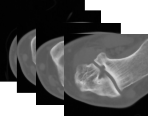
(a)

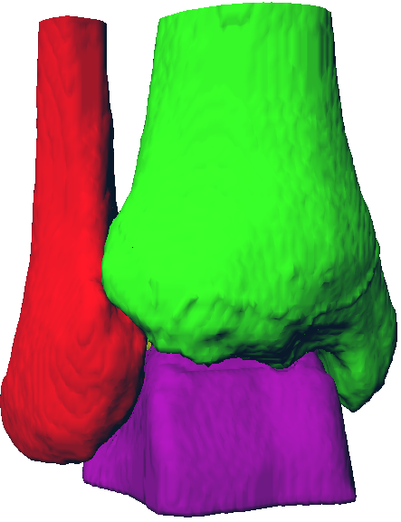
(b)

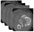
(c)

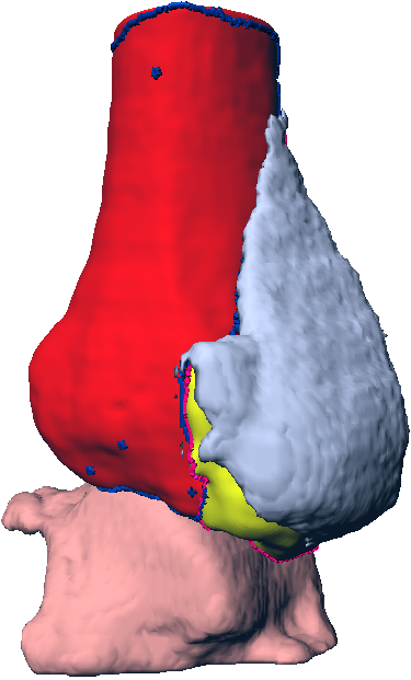
(d)

Figure 3: (a) shows slices from a 3D CT image of an intact ankle joint. (b) shows the segmented tibia, fibula, and talus bone surfaces. (c) shows slices from a 3D CT image of a fractured ankle. (d) shows the segmented bone fragments surfaces. The segmentation from the 3D CT image was performed using the proposed segmentation algorithm.

1. Bone fragment boundaries are especially difficult to demarcate when fragments are abutting other fragments.

2. Intensities for some bone tissues, i.e., cancellous tissue, are the same as that for other soft tissues in the same anatomic region making them difficult to discriminate.

The bone fragment segmentation algorithm takes as input a CT image of the limb and two user parameters: (1) the maximum size of a bone region, and (2) a segmentation sensitivity parameter. The output of this algorithm is a labeled CT image where each unique label corresponds to a unique bone fragment.

The segmentation algorithm proceeds by incrementally classifying pixels from image regions of high-likelihood (cortical tissue) to regions of low-likelihood. To do so, image pixels are initially classified into three sets: (1) non-bone, (2) cortical bone, and (3) non-cortical bone. Connected cortical bone pixel regions are assigned a fragment label and a customized watershed algorithm (Shadid and Willis, 2013), referred to as the Probabilistic Watershed Transform (PWT), merges adjacent pixels into each fragments region. The merge procedure calculates the conditional probability of each candidate pixel given the current segmentation and includes models to specifically address the realization of layered, i.e., lamellar bone tissue structures in CT images, and common fracture phenomenon such as fragment splintering which generates long, thin protrusions of bone tissue that is difficult to otherwise segment. Surfaces are extracted from the segmented image data with the marching cubes algorithm (Hansen and Johnson, 2005). Figures (3(b,d)) show 3D surfaces segmented from CT images of ankle joints for an intact (b) and a fractured (d) ankle joint using the proposed algorithm.

3.4 Partitioning Surfaces

Puzzle-solving requires shapes to be decomposed into shape parts. Similarly, for fracture reconstruction, each segmented bone fragment model must be partitioned into a collection of surface patches to allow the outer surfaces of each fragment surface to be geometrically matched to the template surface, ${\cal S}^{T}$. A surface segmentation algorithm divides fragment surfaces into 3 anatomically distinct groups which greatly reduces the difficulty of the search problem by limiting the number of plausible correct surface matches and thereby improving the reconstruction system performance. The surface mesh partitioning algorithm divides the $k^{th}$ bone fragment surface, $S^{k}$, into a collection of surface patches, $\{s_{1},s_{2}\cdots\}$ , such that $S^{k}=\cup\{s_{1},s_{2}\cdots\}$. Each of the generated surface patches are intended to consist of surface points from only one of three anatomical categories. To do so, the system applies a “ridge walking” algorithm (Willis and Zhou, 2010) which solves this problem geometrically using the fact that the anatomical categories of interest can be discriminated well by dividing the 3D bone fragment surfaces along 3D contours that traverse high-curvature ridges.

3.5 Appearance-Based 3D Surface Classification

A surface classification algorithm must identify the outer, i.e., cortical, surface(s) of each bone fragment from the collection surface patches created by the surface partitioning algorithm. This is a classification problem that is solved using by a classification algorithm, ${\cal C}\left\{s_{1},s_{2}\cdots\right\}$ that extracts the periosteal, i.e., outer, surface, ${\cal S}^{k,o}$, from the set of partitioned surfaces, $\left\{s_{1},s_{2}\cdots\right\}$ from the $k^{th}$ fragment for template-based reconstruction. Our novel classification approach uses CT bone tissue intensity variations in the vicinity the fragment surface to detect the unknown anatomic label of the surface. This is made possible by the fact that cortical, trebecular, cancellous and subchondral bone tissues have distinct intensity ranges and relative thicknesses in the anatomic regions of interest. Unfortunately, intensity variations by machine, patient gender and age (Looker et al., 2009; Felson et al., 1993) require the user to specify training data from within the CT image for reliable output. Figure 4 shows image data from the three anatomic bone regions that must be marked interactively by a user: (1) the diaphysis, made of solid dense cortical bone, (2) the metaphysis, made of a cortical shell and an interior, porous, cancellous bone, and (3) the epiphysis, made of dense subchondral bone. From this data, the automated classification algorithm (Liu, 2012) assigns the partitioned fragment surface patches to one of three semantic labels: (1) “fracture surfaces” (surfaces generated when the bone broke apart), (2) “periosteal surfaces” (surfaces that were part of the outer bone surface), and (3) “articular surfaces” (surfaces that facilitate the articulation of joints). Classification of these surface patches is useful for both bone reconstruction and severity analysis. For reconstruction, the periosteal surfaces for geometric alignment for fragments template-based reconstruction (the approach used in this paper), (2) fracture surfaces allow calculation of surface area produced by a fracture event, which is a valuable objective severity metric, and (3) articular surfaces are particularly medically important in reconstruction. From this data a classifier is constructed and applied to automatically classify the extracted surface patches to these three anatomic labels. A final step merges adjacent periosteal surface patches having the same anatomic label generating the periosteal, i.e., outer, surface, ${\cal S}^{k,o}$. Figure 5 shows classification results for two bone fragments using this approach.

Figure 4: CT appearance of the distal tibia anatomy. Relative to the tibia’s outer surface, the CT intensities vary with characteristic profiles along the inward surface normal for each anatomic region.

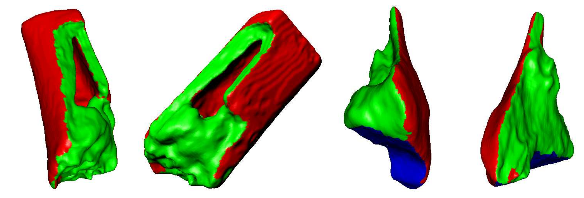
Figure 5: Two views of the surface mesh classification results for two fragments. Red denotes periosteal surface, green denotes fracture surface, and blue denotes articular surface.

3.6 Computational 3D Puzzle Solving

The 3D puzzle-solving algorithm takes as input the $k^{th}$ fragment outer surface patch, ${\cal S}^{k,o}$, and estimates the transformation, $\mathbf{T}_{k}$, that rotates and translates this fragment to it’s original anatomic position within the intact template. A complete virtual reconstruction of the unbroken bone from the bone fragments is achieved by transforming the geometry of each fragment using it’s associated transformation. The intact contra-lateral bone, as represented in the intact CT image, is taken as a reasonable approximation of the unbroken bone after mirroring the geometry across the human bilateral plane of symmetry.

3.6.1 Generic template matching as a puzzle solving approach

Puzzle solving algorithms solve a difficult computational search problem whose goal is to estimate the unknown geometric correspondences between puzzle pieces. This is typically accomplished in two steps: (1) hypothesize geometric matches and (2) test hypothesized matches by evaluating a test statistic; typically the minimized pairwise surface alignment error using the ICP algorithm (Besl, 1992; Chen and Medioni, 1991; Low, 2004; Zhang, 1994)). Each hypothesis has the form: “Fragment surface, ${\cal S}^{k,o}$, corresponds template surface, ${\cal S}^{T}$, at matching surface points $\left\{\mathbf{p}_{k},\mathbf{p}_{T}\right\}$ respectively.” For the $k^{th}$ puzzle fragments the puzzle-solved fragment pose, $\mathbf{T}_{k}$, is taken as the pairwise hypothesis which, after alignment, has the smallest alignment error.

Use of the ICP algorithm to puzzle solve the fracture is both an unreliable and computationally prohibitive option. Reliability is an issue due to the tendency of the ICP algorithm to converge to the closest local minima. Hence, unless the fragments are close to their final anatomic pose in the puzzle solution, it is unlikely their final alignment will be correct. Computational cost is an issue since many fragment surfaces include thousands of samples and finding corresponding surface points is a ${\cal{O}}(N^{2})$ search problem and evaluation of each pairwise correspondence requires a iterative ICP solution which has computational complexity ${\cal{O}}(N^{2})$. Hence the total computational cost of ICP-based reconstruction for one fragment is ${\cal O}(N^{4})$ where $N$ is the number of surface points. For $m$ fragments the complexity increases to ${\cal{O}}(mN^{4})$ ($m\ll N)$ (Arthur and Vassilvitskii, 2006). For our experiments, $N^{4}\sim 10^{20}$ which imposes computational costs high enough to make brute force solutions computationally prohibitive for even very small puzzles.

3.6.2 Surface Descriptor-Based Puzzle Solving

An approach for bone fragment puzzle solving is proposed to make the puzzle solving algorithm computational cost tractable. Descriptor-based puzzle solving approaches extracts descriptors from surfaces and uses these descriptors to hypothesize matches and geometrically align the pieces and use the average alignment error as a statistic to evaluate the likelihood that the hypothesized match is correct. The approach to puzzle-solve the $k^{th}$ fragment, $S^{k,o}$, with respect to intact template, $S^{T}$, consists of five steps:

1. Descriptor Extraction: This step applies a surface descriptor extractor algorithm, ${\cal E}\left\{{\cal S}\right\}$, to puzzle surfaces, ${\cal S}$, to produce a set of Euclidean-invariant surface descriptors. Let ${\cal D}^{T}={\cal E}\left\{{\cal S}^{T}\right\}$ denote descriptors extracted from the template surface and ${\cal D}^{k,o}={\cal E}\left\{{\cal S}^{T}\right\}$ denote descriptors from the $k^{th}$ fragment surface. (see 3.6.3)

2. Generate Matched Features: This step takes in as input the computed descriptors from (1) and outputs a list of matched descriptor pairs: $L_{initial}$. (see 3.6.4)

3. Remove Incorrect Matches: This step takes $L_{initial}$ as input and removes suspected false matches from the initial list and outputs a list of candidate descriptor matches in a new list: $L_{candidate}$. (see 3.6.5)

4. Test Candidate Matches: This step takes in the previously generated list $L_{candidate}$ and outputs a 3D transformation matrix, $\mathbf{T}_{k}$, for each match which aligns the bone fragment to the surface of the intact template.(see 3.6.6)

5. Select The Best Matches: This step determines which of the alignments from the previous step provide the best result and uses these to provide the final puzzle-solved solution. (see 3.6.7)

Applications in surgical planning and image guided surgery require the puzzle solution to be geometrically registered to the coordinate system of the fractured CT image, $\mathbf{I}_{f}$. To this end, an initial alignment is performed between intact template surface, ${\cal S}^{T}$, and the anatomically un-perturbed fragment of the fractured limb which we refer to as the “base fragment.” For tibial plafond fractures the “base fragment,” is typically the uppermost (proximal) bone fragment in the fracture. This initial movement of the template serves to bring the template surface into the coordinate system and vicinity of the bone fragment surfaces improving convergence rates of iterative geometric alignment optimizations. Figure 6 shows a graphical overview of this method for puzzle-solving a clinical bone fracture case.

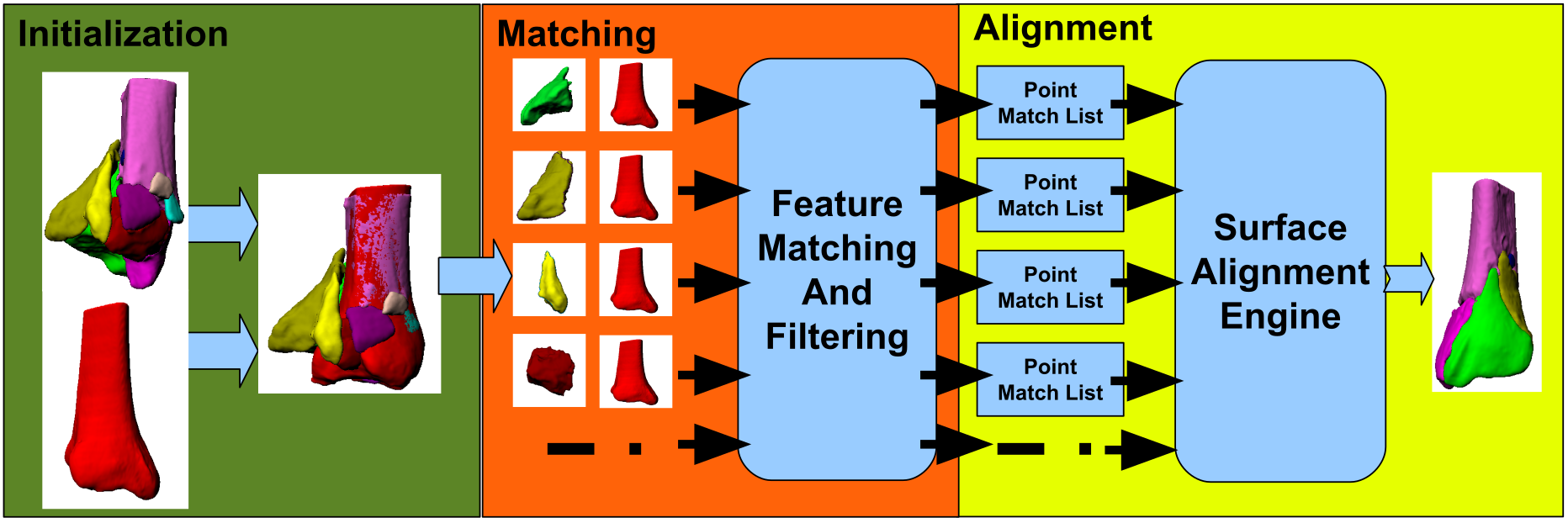
Figure 6: Puzzle solving process: initialization, matching and alignment.

3.6.3 Feature Extraction

While there are many candidate surface descriptors that could be used to compactly characterize local surface patch geometry, this paper adopts the spin image representation (Johnson and Hebert, 1997, 1996) as its surface descriptor. The rationale for this choice is based on the low computational cost this representation affords when performing surface matching. Specifically, spin images converts a nonlinear 3D surface-pair alignment problem into a low-dimensional 2D (spin) image-pair comparison problem (see figure 7d). Spin images of two identical surface patches in arbitrary pose generate produce identical 2D spin images. As mentioned in § 3.1, use of spin images significantly reduces the complexity of comparing surface shapes by reducing the computational complexity from polynomial time ${\cal{O}}(kN^{2})$(ICP) to linear ${\cal O}(N_{overlap})$ for spin image pair having $N_{overlap}$ overlapping pixels (2D-image subtraction). Unfortunately, matching spin images does not solve the complete alignment problem and requires estimation of a single additional parameter: rotation about the corresponding surface normals. Hence, spin images provide a compact, yet imperfect, Euclidean invariant representation of the shape of a bone fragment surface.

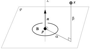
(a)

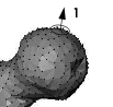
(b)

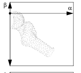
(c)

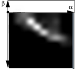
(d)

Figure 7: (a) Oriented surface point $\mathbf{p}$ with its normal n and the tangent plane $p$, one of its neighbor point $\mathbf{x}$ on the fragment surface and $(\alpha$,$\beta)$ are computed values for point $\mathbf{x}$ respect to point $\mathbf{p}$ ; (b) shows point $\mathbf{p}$ on the bone surface and its neighbor points; (c) Plotted neighbor points on the $(\alpha,\beta)$ grid; (d) Computed spin image for out of (c) Johnson and Hebert (1997).

3.6.4 Generate Matched Descriptors

Let $L_{initial}$ denote the list of initial hypothesized matches where each match is specified by an index pair $\left\{i,j\right\}$ indicating that the $i^{th}$ surface descriptor from the template, ${\cal D}_{i}^{T}$, is hypothesized to correspond to the $j^{th}$ surface descriptor from the $k^{th}$ fragment’s outer surface ${\cal D}_{j}^{k,o}$. Evaluation of the correspondence hypotheses is accomplished by calculating the value of a similarity function $C_{sp}(P,Q)$ to detect similar surface matches. To avoid biases in descriptor matching, the proposed function combines statistical correlation and sample size into this similarity function.

Our similarity function uses the normalized linear correlation coefficient, $R_{sp}(P,Q)$, to measure descriptor similarities as shown in equation ((1)) which assigns a score of 1 for a perfect match and scores can range from (-1, 1). Given two spin images $P$ and $Q$ with $N_{bin}$ bins (number of pixels in the image ), denote $p_{i}=P(\alpha,\beta)$ as the $i^{th}$ spin image intensity value from spin image $P$, similarly, denote $q_{i}=I(\alpha,\beta)$ as the $i^{th}$ spin image intensity value from spin image $Q$. With this notation, the linear correlation coefficient, $R_{sp}(P,Q)$, is computed as shown in equation (1):

$$R_{sp}(P,Q)=\frac{N_{bin}\underset{i}{\sum}p_{i}q_{i}-\underset{i}{\sum}p_{i}\underset{i}{\sum}q_{i}}{\sqrt{\left(N_{bin}\underset{i}{\sum}p_{i}^{2}-\left(\underset{i}{\sum}p_{i}\right)^{2}\right)\left(N_{bin}\underset{i}{\sum}q_{i}^{2}-\left(\underset{i}{\sum}q_{i}\right)^{2}\right)}}$$ (1)

When $R_{sp}$ is close to 1, the images are similar, when $R_{sp}$ is close to -1 the images are different. Unfortunately, this metric is biased since each spin image may have different $(\alpha,\beta)$ dimensions. Hence good matches may be found when spin images have similar values over small overlapping $(\alpha,\beta)$ regions. On the other hand, two spin images with a large area of overlap may be assigned a lower $R_{sp}$ value but exhibit widespread similarities.

To address biases $R_{sp}(P,Q)$ the similarity function $C_{sp}(P,Q)$ proposed in (Johnson and Hebert, 1997, 1996) was used as shown in equation (2). This metric is well-suited because it considers both the correlation, i.e., match fidelity, and also the number of matching or overlapping pixels, $N_{overlap}$ , as part of the final matching score.

$$C_{sp}\left(P,Q\right)=\left(\text{{atanh}}\left(R_{sp}\left(P,Q\right)\right)\right)^{2}-\lambda\left(\frac{1}{N_{overlap}-3}\right)$$ (2)

The resulting similarity function weights the correlation $R_{sp}$ against the variance intrinsic to the correlation coefficient which increases as the amount of overlap in the two spin images increases. This is accomplished via a change of variables commonly referred to as "Fisher’s z-transformation" (Fisher, 1915) which uses the hyperbolic arctangent function to transform the distribution of the correlation coefficient into an approximately normal distribution having constant variance $\frac{1}{N_{overlap}-3}$ . This allows the similarity metric (2) to be formed that strikes a compromise between good correlations (term 1) and sufficient evidence, i.e., measurements to trust the computed correlation (term 2) to better detect reliable matches. The parameter $\lambda$ is used to control the relative weight of the expected value of the correlation coefficient and the variance of this statistic to produce a final similarity score. (Johnson and Hebert, 1997, 1996) mention that $\lambda$ controls the point at which the overlap between spin images dominates the value of the similarity metric for two spin images. When the overlap is much larger than $\lambda$, the second term in equation (2) becomes negligible. In contrast, when the overlap is much less than $\lambda$, the second term dominates the similarity measure. Therefore, $\lambda$ should be the expected overlap between spin images. In this paper, $\lambda$ is automatically computed for each surface match by computing average number of non-black pixels for all the spin images generated from that fragment and setting $\lambda$ to half of the average value.

3.6.5 Removing Incorrect Matches

Due to the noise from image data and errors from segmentation and classification algorithms, the initial list of matches $L_{initial}$ often contains many false hypothesized surface point correspondences. Since careful analysis of these matches is computationally expensive, we propose an alternative approach to detect incorrect hypotheses that significantly improves performance. To do so we consider multi-hypothesis consistency constraints to efficiently eliminate implausible solutions.

Conceptually, the idea here is that each fragment has a single unique Euclidean transformation that brings the fragment to it’s original anatomic location, $\mathbf{T}_{k}$. Hence, if multiple hypotheses from the same fragment are made, those that are correct must have nearly the same value for $\mathbf{T}_{k}$. Towards this end, evaluated hypotheses for the $k^{th}$ can be used to cross-validate other hypotheses from the same fragment. However, rather than performing the computationally expensive alignment required to compute $\mathbf{T}_{k}$, we use similarity as provided by spin image surface descriptors to reject large numbers of incorrect hypotheses.

Let $\left\{{\cal D}_{i}^{T},{\cal D}_{j}^{k,o}\right\}$ and $\left\{{\cal D}_{l}^{T},{\cal D}_{m}^{k,o}\right\}$ denote descriptor pairs $\{i,j\}$ and $\{l,m\}$ from the list $L_{initial}$ computed from surface points are $\left\{\mathbf{p}_{i}^{T},\mathbf{p}_{j}^{k,o}\right\}$ and $\left\{\mathbf{p}_{l}^{T},\mathbf{p}_{m}^{k,o}\right\}$. If both hypotheses are correct, then the surface point pairs should be geometrically consistent, i.e., the distance between $\mathbf{p}_{j}^{k,o}$ and $\mathbf{p}_{m}^{k,o}$ should be equal to the distance between $\mathbf{p}_{i}^{T}$ and $\mathbf{p}_{l}^{T}$. This constraint can be directly validated using spin image coordinates in a geometric consistency test. If the two matches satisfy equation ((3)), we consider them to be geometrically consistent matches which means both of them may be true matches.

$$\left|{\cal D}_{i}^{T}\left(\mathbf{p}_{j}^{k,o}\right)-{\cal D}_{j}^{k,o}\left(\mathbf{p}_{i}^{T}\right)\right|-\left|{\cal D}_{l}^{T}\left(\mathbf{p}_{m}^{k,o}\right)-{\cal D}_{m}^{k,o}\left(\mathbf{p}_{l}^{T}\right)\right|<D_{gc}$$ (3)

Where $D_{gc}=2\gamma_{intact}$ where $\gamma_{intact}$ is the resolution of the intact template, i.e., the average edge length of the edges from the intact template surface mesh.

When the initial match list is constructed, list elements are sorted by decreasing similarity score, $C_{sp}$. Inconsistent elements are removed by splitting the list $L_{initial}$ into two parts at its midpoint. The first list contains matches having higher similarity scores and the second contains matches that having lower similarity scores. We consider one match from each of the two lists respectively form pairwise correspondence hypotheses. The geometric consistency condition is evaluated for the pair of correspondences. If they both satisfy the consistency condition, we keep both matches. Otherwise, we keep the match that has a higher similarity score and discard the other match. After evaluating all matches in both lists, the remaining matches are placed in the sorted list referred to as $L_{candidate}$.

3.6.6 Test Candidate Matches

The reduced set of hypotheses in the $L_{candidate}$ set are now evaluated by calculating their 3D surface alignment error. As mentioned previously, this is a computationally expensive step involving nonlinear optimization via the ICP algorithm which is further known to suffer from erroneous solutions when the initial transformation, $\mathbf{T}_{0}$, for optimization lies far from the true value, $\mathbf{T}_{k}$. Our surface descriptor matches serve to significantly reduce computation here by performing a coarse initial alignment which provides a good initial guess for 5 of the 6 unknown transformation parameters, specifically the (3) translation parameters and (2) of the three unknown rotation parameters. For a given match, the alignment proceeds in two steps:

1. Coarse Surface Alignment: For each likely descriptor match hypothesis $\left\{{\cal D}_{i}^{T},{\cal D}_{j}^{k,o}\right\}$ an initial transform, $\mathbf{T}_{0}$, is calculated which translates the fragment surface,${\cal S}^{k,o}$, to make it’s surface point, $\mathbf{p}_{j}^{k,o}$, correspond with the template’s surface point $\mathbf{p}_{i}^{T}$ and simultaneously rotates the fragment surface to make the fragment and template surface normals also correspond at these points.

2. Refined Surface Alignment: Using the initial transform $\mathbf{T}_{0}$, we run the ICP algorithm to compute final 3D alignment error.

In this way hypotheses can be used that may not be exactly correct and in cases where the hypothesis is “close,” the ICP algorithm is still likely to converge to the correct alignment.

3.6.7 Selecting The Best Matches

Figure (8) illustrates how the alignment process uses a hypothesized surface correspondence to align a fragment to the intact template. For a given fragment, each hypothesized surface correspondence is evaluated in the sequence given by the match score from §(3.6.5) starting at the highest score. Each evaluation aligns a fragment to the intact template using the three alignment steps specified in the three previous section. However, if the algorithm goes through all three steps for every match, the reconstruction process is very time-consuming. To reduce computation each alignment step includes predefined conditions to determine whether the system should continue to evaluate the match or discard the match and try a new hypothesized match. The local alignment error is used to control the process. Because the computational cost increases in each step, the alignment error threshold values are smaller (stricter) for each step. In this paper, the threshold values are $4\gamma_{intact}$ for step one, $2\gamma_{intact}$ for step two, and $\gamma_{intact}$ for step three. Finally, when one match is accepted by all three steps the output position from step three is considered as the final alignment for the fragment.

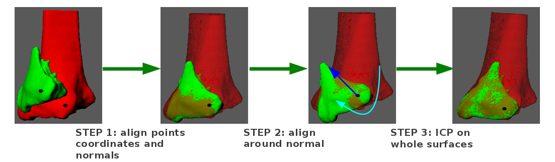
Figure 8: An example of alignment using the surface alignment engine. The red bone is the intact template, the green bone is one of the fracture fragment. The two black points on both surfaces are matched surface points.

3.6.8 System Enhancements

Several software enhancement tools are introduced to help improve the quality of the 3D puzzle-solved solutions and to help reduce the time necessary to compute these solutions. These enhancement tools include: (1) surface sampling, (2) using occupied regions, (3) Mean Curvature Histogram Biased Search, and (4) global fragment alignment optimization. The following sections (3.6.9, 3.6.10, 3.6.11, 3.6.12) discuss each tool in detail.

3.6.9 Surface Sampling

The intact template and the fragment surfaces often consists of a large number of surface points. Computing spin images for every point on these surfaces is a time-consuming task. In order to improve the speed of the puzzle-solving algorithm, uniform sub-sampling is applied on both the intact template and the fragment surfaces. Surface points are randomly selected on the fragment with a constraint that the distance between any two sampled surface points are greater than a predefined sampling distance $\triangle s$. The larger $\triangle s$ value computes fewer sampled points on the fragment surface and smaller value computes more sampled points on the fragment surface. Spin images are only computed for those sampled surface points on the intact template and the fragment surfaces. In this paper, the sub-uniform sampling distance for each fragment is set to $\triangle s=1.5\gamma_{intact}$, and $\gamma_{intact}$ is the average edge length of edges on the intact template.

3.6.10 Using Occupied Regions

The concept of occupied regions allows for significant performance improvements by further reducing the spin images computed on the intact template. Since part of the intact template surface has already been aligned to the base fragment, these points should be excluded from the matching. We mark these surface points on the intact template surface as “occupied”, and spin images are only computed for surface points inside the “unoccupied” regions of the intact template. This significantly reduces the search space for the matching process. Occupied points on the intact template are flagged using the following condition: the intact surface point, $\mathbf{v_{\textrm{j}}^{\textrm{t}}}$, is marked as “occupied” if its distance to the closest aligned fragment surface is less than $2\gamma_{intact}$.

3.6.11 Mean Curvature Histogram Biased Search

To reduce the number of spin images computed for both the intact template and fragment surfaces, an approach called mean curvature histogram biased search is used. Here we bias the search to emphasize regions having discriminative shape by selectively computing descriptors in locations where the mean surface curvature is large, i.e., highly curved surface locations. The goal is to focus on calculating surface descriptors that are more easily matched and have fewer candidate correspondences. Using these locations allows computation to focus on regions that carry more information regarding the unknown puzzle solution. Towards this end, each descriptor is attributed with an estimate of the surface mean curvature at the associated surface point. We then randomly select points uniformly from the distribution of observed curvatures which drastically reduces the number of spin images computed. Further, when forming pairwise hypotheses we only create hypotheses for points pairs whose mean surface curvature are similar. This approach greatly reduces the computational cost of the puzzle solving algorithm and improves performance of the reconstruction without an observed sacrifice in solution accuracy.

3.6.12 Global Optimization of Fragment Alignment

Global alignment seeks to simultaneously optimize all unknown transformation parameters of the puzzle-solved fragments. This serves to correct minor discrepancies in the position of misaligned fragments by fitting together adjacent fragments onto the template surface in the final reconstruction results. This is accomplished by perturbing fragment transformation values away from the current puzzle solution and performing ICP simultaneously using the global alignment algorithm of (Pulli, 1999). This approach seeks to simultaneously equalized the surface alignment error equally across all fragments and enforce the restriction that fragment-and-template surface correspondences are unique, i.e., each template surface point can only correspond with points from a single fragment (as described in 3.6.10). Since the perturbations are small, this procedure serves to make small adjustments each fragments final surface position on the intact template and minimize fragment-to-fragment surface overlap. This process can improve the pose of slightly misaligned fragments in the final puzzle solved solution.

3.7 Post-Reconstruction Analysis

The post-reconstruction analysis is the final output of the system. The analysis tools are integrated into the system and allow users to analyze the reconstruction result and help users better understand the fracture case. The analysis consists of two components: (a) analysis of the geometric accuracy of the aligned fragments and (b) analysis of the severity of the bone fracture. The first component provides a table containing alignment information, such as sampled, matched, and unmatched points, and a histogram of alignment error for each fragment. The second component is a fracture severity report which contains quantitative values for several key factors for each fragment which are known to be indicators of fracture severity, such as fracture surface area. Although visual assessment of 3D reconstruction result is valuable to users, these analysis tools provide quantitative information which can help users objectively interpret the fracture case.

Analysis of the geometric accuracy of the reconstruction is accomplished by measuring the point-to-plane distance from each vertex of the fragment surface to the plane of the closest triangle on the intact template. These distances are averaged to compute alignment error for each fragment. The post-reconstruction analysis report includes a table of alignment information and a table of histograms that show the distribution of alignment errors for each fragment.

Our system provides histograms of the alignment error, providing users with more detailed statistical information that relate to the quality of the fragment alignment. Moreover, the system makes it possible to visualize the location and magnitude of the alignment errors as a spatial distribution on the fragment surface. Interactions are available from the histogram plot which allow the user to select a range of error values. Once selected, the errors associated with these values are visualized spatially across the surface of the fragment as shown in figure 9. These tools are valuable for understanding the quality of the geometric reconstruction results and understanding the complex geometric inter-dependencies of a highly-fragmented bone fracture.

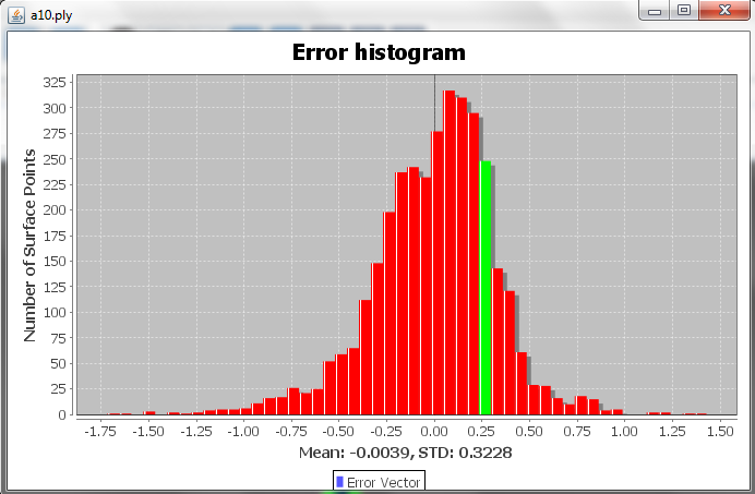
(a)

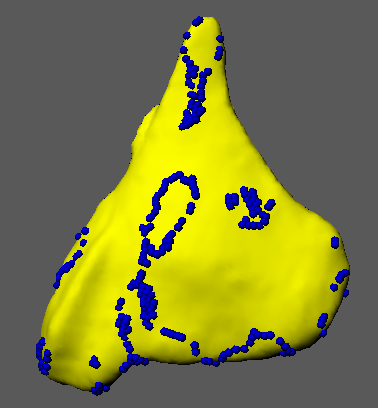
(b)

Figure 9: (a) shows a histogram of alignment errors where the bin of vertices having an error of approximately 0.25 $mm$ has been selected (green). (b) shows a visualization of the spatial distribution surface points (blue spheres) which have these errors on the fragment surface.

Severity assessment for bone fractures is heavily influenced by a number of related key factors. One contribution of this paper is to provide quantitative values for some of these key factors which are heretofore unavailable in any other fracture analysis software. Figure 10 shows an example of the severity assessment report which includes computed values of key factors for each fragment in case one. The following list describes the values provided in the severity assessment report in detail:

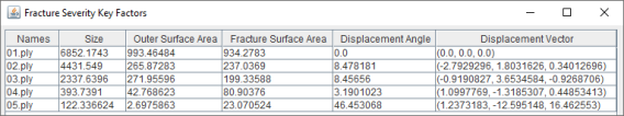
Figure 10: A severity assessment report is shown which includes values for several quantities that are known to be key factors in determining fracture severity.

1. Fragment Volume: This is 3D volume of the region enclosed by the fragment surface (shown as “Size” in the severity report table). This information is useful in determining if the fragment is structurally stable and useful in clinical reconstruction, i.e., can it be used for fixation, or is too small to be used in reconstruction.

2. Fragment Fracture Surface Area: The area of the fragment fracture surface is a major factor in determining fracture severity as shown in (Beardsley et al., 2005). The area of the fracture surface generated is directly related to the energy that the fractured bone absorbed during the fracture event.

3. Fragment Displacement: The fragment displacement is the 3D translation vector that moves the centroid of the fragment, which indicates how far a fragment has moved or dispersed during the fracture event.

4. Angular Dislocation: The angular dislocation of the fragment is the angle between the principal axis of the bone fragment in its original position and the principal axis of the bone fragment in its reconstructed position.

These quantities are closely linked to fracture severity and the displayed values may allow users to more accurately and objectively estimate fracture severity. Computation of fracture surface areas from 2D or 3D CT images are difficult and the results are often unreliable. Here, the total fracture surface area can be calculated more accurately after the 3D fragment surfaces are segmented and anatomically classified. Physicians have no way to quantitatively estimate fragment displacement and angular dislocation from image data. Current approaches rely upon the physician’s visual assessment and experience. For high energy fracture cases, accurately assessment of these values are difficult. Since the proposed system has unique capabilities to compute the original and reconstructed position for each bone fragment, the key factors shown are inaccessible from any other source. Values uniquely available from the proposed software are fragment displacement, angular dislocation, and the surface area for the fragment outer surface and fracture surfaces.

4 Results

The bone reconstruction system was used to reconstruct six clinical fracture cases which range from low energy fracture events such as 1.5 foot fall, to high energy fracture events such as a 50 mph car accident. The patient data, injury cause, and the Orthopedic Trauma Association (OTA) classification for each case is shown in Table 1. Since these are real clinical cases, the patient names have been removed to protect their privacy. All of the six cases were assigned a numerical severity score ranging from (1-100) by three well-trained surgeons based on their personal experience and subjective inference shown in column $C_{1},$$C_{2}$, and $C_{3}$ of Table 1. Of particular note is the high variance across clinicians of these classifications, consistent with the findings of (Humphrey et al., 2005), highlighting the need for objective measures of fracture severity.

Case #	Sex	Age	AO/OTA classification	Injury mechanism	C1	C2	C3	Avg
1	F	38	C32	MVA (50 mph)	60	55	60	58
2	M	21	B13	Fall (30 ft)	50	60	58	56
3	F	42	C21	MVA (30 mph)	62	80	79	74
4	M	20	C13	ATV	6	15	32	18
5	M	24	C23	Fall (12 ft)	55	57	62	59
6	M	34	C11	Fall (18 ft)	70	65	77	71

Table 1: Patient data, injury cause, OTA classification, and severity scores by three surgeons for each case. The higher severity scores indicate higher fracture severity.

The section 4.1 shows the additional reconstruction results for each case. For all six cases, the fragment and intact surfaces were segmented, partitioned and classified using the methods described in 3.3, 3.4 and 3.5 to provide the data necessary to puzzle-solve each fracture case.

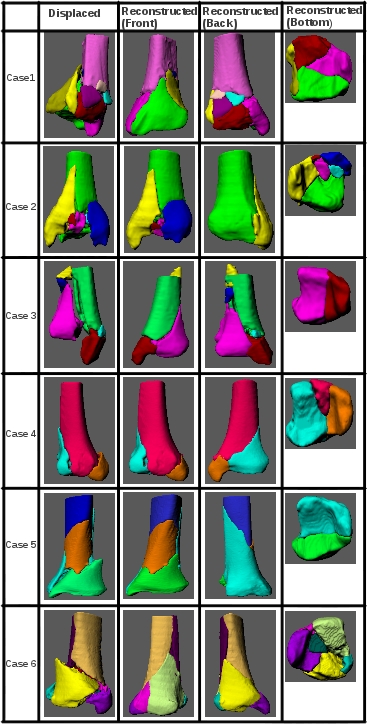
Figure 11: Six clinical tibia plafond fractures are puzzle-solved. The original fractured positions for the fragments are shown in the left column and three different views of reconstructed fragments are shown in the remaining columns.

Figure 11 shows the displaced positions and three different views of reconstructed fragments for all six clinical fractures. By visual assessment of the reconstruction results, all cases were reconstructed successfully with the exception of case three.

Case ID	Completion time (sec)	Number of points on intact	Global Alignment Error (mm)
1	140	24935	0.23
2	220	45529	0.27
3	272	50539	0.32
4	90	33630	0.34
5	430	68160	0.33
6	650	117549	0.27

Table 2: Puzzle solving performance: the time needed to run puzzle-solving algorithm for the fracture case on a 2.4GHz, 4GB RAM laptop and the global alignment error.

Column 3 of Table 2 summarizes the global alignment errors for all six cases. From the table, we can see that global alignment error after the construction for all six cases are relatively small (< 0.35mm), demonstrating higher accuracy than competing methods (Okada et al., 2009; Moghari and Abolmaesumi, 2008; Fürnstahl et al., 2012). Table 2 shows the time needed to run the puzzle-solving algorithm. These reconstruction times were recorded on a 2.4GHz, dual-core laptop with 4GB of RAM. The reconstruction time recorded for each case includes time spent for computing spin images, matching spin images, and aligning fragment surfaces. The semi-automatic steps of the reconstruction: surface partitioning, surface patch classification, and puzzle solving initialization are not included here. From the table we can see that as the number of points on the intact template increases so does the time required for reconstruction. This is reasonable because more points result in more hypotheses in the puzzle solving process. Indeed, the recorded reconstruction time is influenced by several variables such as the number of spin images computed from the intact template and the fragment surfaces, number of fragments, number of iterations of the ICP algorithms, etc. In §4.2 we discuss a small modification made to boost performance. Table 4 in the Appendix records the results of each fragment processed by the system.

4.1 Notes on Each Case

Each of the six cases processed by our system supplies valuable insight to the versatility of the reconstruction method. All cases except Case 3 (which will be explained below) were deemed successful due to good visual geometric agreement and via the value of the global alignment error. Case 1 contained ten unique fragments to place, yet still achieved a global error of 0.23mm. This demonstrates the efficacy of the proposed method even in complex fracture cases. Case 2’s fragment A4 underwent a displacement magnitude of almost five centimeters (48.98mm), which is substantially large compared to the total size of the tibia’s epiphysis. Despite this, Case 2’s reconstruction was successful, demonstrating the resilience of the proposed reconstruction approach to local minima. Case 3 was the only unsuccessful reconstruction of all test cases. Its fragment A2 clipped through the base fragment (A1) despite the anatomical impossibility. This may be attributed to the low resolution of Case 3’s CT DICOMs. It had the lowest resolution at 0.683mm per pixel which would increase the likelihood of false positive matches in the generated spin images. Case 4 and 5 consist of a small number of fragments (3 and 4 respectively). This resulted in higher points per fragment to match, increasing the computational cost of the puzzle solution. However, reconstruction for this case was successful and demonstrates the system’s capacity for processing large fragment surface matches. Case 6 was unique in its low percentages of outer surface area on each fragment. The reconstruction was still successful despite the smaller amount of points to match per fragment.

Case	$t_{tl}$ w/o accel. (min)	$t_{tt}$ w/ accel. (min)	Avg match time w/o accel.(sec)	Avg matching w/ accel.(sec)	$n_{i}$ w/o accel.	$n_{i}$ w/ accel.	# Points On Template
1	3	1.5	11	0.3	3750	1125	24935
2	6	4.5	15	0.8	5065	802	45529
3	8	5	16	1.2	5320	1913	50539
4	2.5	1	10	0.2	2509	897	33630
5	20	6	34	2.4	8890	4135	68160
6	31	16	52	3.5	16829	3120	117549

Table 3: Computational performance observed for each case using the system enhancements discussed in §3.6.11.

4.2 Performance Improvements

As mentioned in §3.6.11, the mean curvature histogram biased search algorithm significantly improves the speed of the automatic puzzle-solving algorithm by reducing the number of spin images computed for both the intact template surface and the fragment surfaces. The puzzle-solving algorithm is a complex process which consists of many steps, and the time spent for the reconstruction is affected by intermediate steps such as computing the spin images for the intact template and the fragment surfaces, matching spin images, and aligning fragment surfaces to the intact template. In order to better understand the improvements, the following equation (4) details the time spent for reconstruction for each step.

$$t_{tl}=t_{o}+n_{i}t_{s}+\left(t_{s}n_{f}+t_{m}+t_{f}+t_{a}\right)M_{f}$$ (4)

In this equation, $t_{o}$ denotes the time spent for processing the intact template before computing the spin images on the intact template such as surface sampling, computing occupied regions and computing the mean curvatures for the intact template. The term $n_{i}t_{s}$ denotes the time spent to identifying feature points on the intact template and compute their spin images. The term $t_{s}n_{f}$ denotes the time spent computing descriptors on the fragment surfaces. The term $t_{m}$ denotes time spent generating hypothesized surface correspondences which is affected by $n_{f}$ and $n_{i}$. The term $t_{f}$ denotes the time spent removing false matches. The term $t_{a}$ denotes time spent aligning the fragment surface to the intact template which is affected by number of hypothesized correspondences being tested. The term ${\color[rgb]{0,0,1}K}$ denotes the number of fragments in the fracture case. The major factors that impact the total reconstruction time are $n_{f}$, the number of spin images computed on the fragment surface, and $n_{i}$, the number spin images computed on the intact template. The mean curvature histogram approach in §3.6.11 reduces the total reconstruction time by reducing both $n_{i}$ and $n_{f}$ significantly Table 3 shows the quantitative values for total reconstruction time, $t_{tl}$, average time spent for matching spin images and filtering matches, $t_{m}+t_{f}$, and $n_{i}$ for each case. Note that acceleration provides roughly an order of magnitude decrease on computation time for matching and reduces the total reconstruction time, including user interaction, by about 50%. Experimental reconstructions were conducted using a laptop computer with 2.4GHz dual core CPU with 4GB memory.

Our accelerated reconstruction times are significantly shorter than those reported in similar systems. Work in (Fürnstahl et al., 2012) reported an average total reconstruction time of 83 minutes which is approximately 5 times longer than our worst-case clinical reconstruction (16 mins) and more than 10 times longer than the average time it requires for reconstruction across our 6 cases (~5 mins 45 secs). Unfortunately the performance in time of the methods described in (Okada et al., 2009; Moghari and Abolmaesumi, 2008) are not reported.

5 Conclusion

The proposed system is capable of virtually reconstructing broken bone fragments for complex bone fracture cases, which is currently an unsolved problem in automatic puzzle-solving algorithms and difficult to achieve using manual methods. The bone reconstruction system designed in this paper enables users to understand fracture cases from both 2D (CT image) and 3D (fragment surface) imagery. The system represents a unique combination of state-of-the-art 2D/3D image processing and surface processing algorithms. The software is a comprehensive reconstruction tool that guides users from the first step, i.e., segmenting raw CT image data, to the last step, i.e., generating quantitative, critical information about the fracture’s severity. Finally, 3D visualization of fragment surfaces can provide important information for surgical treatment, especially for articular fractures which often have a poor prognosis.

The system demonstrates the efficacy of spin image reconstruction in bone fractures from various fracture events with a wide variety of traits. Reconstruction was successful in bone fractures with both many and few fragments (Cases 1, 4, and 5), fractures where fragments have undergone large displacements (Case 2), and fractures where little intact outer surface area remains (Case 6). The reconstruction only suffers in cases where the source CT images were generated at low resolutions (greater than 0.5mm per pixel, Case 3). In each case, global alignment errors less than 0.35mm were achieved.

With the detailed fracture analysis offered by this tool, it could potentially improve surgical treatment, as previously explored in (Thomas et al., 2010, 2011). The system represents a significant step towards assisting physicians in classifying fracture severity which is especially difficult in high-energy fracture cases. Use of quantitative metrics in conjunction with visual assessment promises to reduce variability in fracture severity classification and may serve to build consensus in these difficult cases. The puzzle-solving algorithms and their integration as a software system represent significant advancements toward improving the treatment of comminuted tibial plafond fractures and it is entirely possible this technology can be applied to other problematic limb fracture cases. While not directly discussed in this article we also note that the computational 3D puzzle solving framework provides a heretofore unavailable patient-specific blueprint for fracture reconstruction planning. Having a suitable blueprint for restoring the original anatomy, it becomes possible for the surgeon to pre-operatively explore less extensive surgical approaches and to attempt new minimally invasive surgical approaches.

Appendix A. Summary of per-fragment results for reconstruction

Table 4 records the results of each fragment processed by the system. Displacement and displaced angle demonstrate how far each fragment moved from its reconstructed position in the fracture event. The fracture surface area provides insight to the energy of the event. The percentage of outer surface area to total surface area provides insight to the difficulty of finding matches to the intact bone template.

	Fragment	Displacement (mm)	Displaced Angle (deg)	Outer Surface Area (mm2)	Fracture Surface Area (mm2)	% Outer to Total Area
Case 1	A1	0	0	274.5	446.4	45.62
	A2	7.201	20.40	91.96	115.5	44.33
	A3	2.256	6.541	4.037	4.382	47.95
	A4	13.07	29.19	126.8	223.7	26.18
	A5	6.324	17.60	43.86	48.68	47.40
	A6	8.566	15.29	11.74	11.21	51.16
	A7	13.30	28.38	133.7	236.6	36.11
	A8	2.948	5.765	12.63	15.70	44.58
	A9	12.98	26.25	74.39	164.2	31.18
	A10	16.89	37.34	29.58	29.35	50.20
Case 2	A1	0	0	949.8	993.9	48.87
	A2	6.838	12.19	389.8	338.9	53.49
	A3	7.481	20.03	218.8	159.3	57.87
	A4	48.98	85.92	17.10	108.1	13.66
	A5	29.78	178.4	44.0	29.62	59.78
	A6	21.59	44.29	7.449	15.62	32.29
Case 3	A1	0	0	2331	1487	61.05
	A2	38.12	62.87	216.2	117.4	54.93
	A3	35.15	36.51	91.63	110.9	45.24
	A4	22.59	10.79	1848	1143	61.79
	A5	29.15	25.26	55.65	62.12	47.25
	A6	83.56	47.64	574.9	907.8	38.77
Case 4	A1	0	0	1924	1754	52.31
	A2	3.545	4.931	680.8	859.0	44.21
	A3	3.734	12.25	380.6	464.2	45.05
Case 5	A1	0	0	463.3	438.9	51.35
	A2	2.987	5.175	851.9	755.6	52.99
	A3	1.631	5.101	303.3	332.8	47.68
	A4	15.79	23.12	330.6	463.5	41.63
Case 6	A1	0	0	246.8	246.0	50.08
	A2	5.979	16.89	17.26	31.14	35.66
	A3	1.015	3.992	108.7	159.0	40.61
	A4	2.778	20.08	93.70	292.6	24.26
	A5	2.887	14.27	28.03	54.24	34.07
	A6	7.564	19.17	10.03	51.67	16.26
	A7	1.686	8.294	97.33	249.0	28.10
	A8	8.417	23.45	46.44	133.8	25.77

Table 4: Summary of results for all fragments of the six test cases.

References

- Albrecht and Vetter (2012) Albrecht, T., Vetter, T., 2012. Automatic fracture reduction, in: Lecture Notes in Computer Science. Springer Berlin Heidelberg, pp. 22–29.
- Anderson et al. (2008a) Anderson, D., Mosqueda, T., Thomas, T., 2008a. Quantifying tibial plafond fracture severity: Absorbed energy and fragment displacement agree with clinical rank ordering. Journal of Orthopaedic Research 26, 1046–1052.
- Anderson et al. (2008b) Anderson, D.D., Mosqueda, T., Thomas, T., Hermanson, E.L., Brown, T.D., Marsh, J.L., 2008b. Quantifying tibial plafond fracture severity: Absorbed energy and fragment displacement agree with clinical rank ordering. Journal of Orthopaedic Research 26, 1046–1052. doi:10.1002/jor.20550.
- Arthur and Vassilvitskii (2006) Arthur, D., Vassilvitskii, S., 2006. Worst-case and smoothed analysis of the ICP algorithm, with an application to the k-means method, in: 47th Annual IEEE Symposium on Foundations of Computer Science, IEEE. doi:10.1109/focs.2006.79.
- Beardsley et al. (2005) Beardsley, C.L., Anderson, D.D., Marsh, J.L., Brown, T.D., 2005. Interfragmentary surface area as an index of comminution severity in cortical bone impact. Journal of Orthopaedic Research 23, 686–690. doi:10.1016/j.orthres.2004.09.008.
- Besl (1992) Besl, P.J. & McKay, N., 1992. A method for registration of 3-d shapes. IEEE Trans. PAMI 14, 239–256.
- Brumback and Jones (1994) Brumback, R., Jones, A., 1994. Interobserver agreement in the classification of open fractures of the tibia. The results of a survey of two hundred and forty five orthopaedic surgeons. The Journal of Bone and Joint Surgery 76, 1162–1166.
- Charalambous et al. (2007) Charalambous, C., Tryfonidis, M., Alvi, F., Moran, M., Fang, C., Samaraji, R., Hirst, P., 2007. Inter- and intra-observer variation of the schatzker and AO OTA classifications of tibial plateau fractures and a proposal of a new classification system. The Journal of Bone and Joint Surgery 89, 400–404.
- Chen and Medioni (1991) Chen, Y., Medioni, G., 1991. Object modeling by registration of multiple range images, in: Proceedings. 1991 IEEE International Conference on Robotics and Automation, IEEE Comput. Soc. Press. doi:10.1109/robot.1991.132043.
- Chowdhury et al. (2009) Chowdhury, A., Bhandarkar, S., Robinson, R., Yu, J., 2009. Virtual multi-fracture craniofacial reconstruction using computer vision and graph matching. Computerized Medical Imaging and Graphics 33, 333–342.
- Cimerman and Kristan (2007) Cimerman, M., Kristan, A., 2007. Preoperative planning in pelvic and acetabular surgery: The value of advanced computerised planning modules. Injury 38, 442–449.
- van Eijnatten et al. (2018) van Eijnatten, M., van Dijk, R., Dobbe, J., Streekstra, G., Koivisto, J., Wolff, J., 2018. CT image segmentation methods for bone used in medical additive manufacturing. Medical Engineering & Physics 51, 6–16. doi:10.1016/j.medengphy.2017.10.008.
- Felkel et al. (2001) Felkel, P., Bruckschwaiger, M., Wegenkittl, R., 2001. Implementation and complexity of the watershed-from-markers algorithm computed as a minimal cost forest. Computer Graphics Forum 20, 26–35. doi:10.1111/1467-8659.00495.
- Felson et al. (1993) Felson, D.T., Zhang, Y., Hannan, M., Anderson, J., 1993. Effects of weight and body mass index on bone mineral density in men and women, the framingham study. Journal of Bone and Mineral Research 8, 567–573.
- Fisher (1915) Fisher, R.A., 1915. Frequency distribution of the values of the correlation coefficient in samples from an indefinitely large population. Biometrika 10, 507–521. URL: http://www.jstor.org/stable/2331838.
- F.Meyer (1994) F.Meyer, 1994. Topographic distance and watershed lines. Signal Processing 38, 113–125.
- Freeman H (1964) Freeman H, G.L., 1964. Apictorial jigsaw puzzles: The computer solution of a problem in pattern recognition. IEEE Transactions on Electronic Computers EC-13, 118–127.
- Fürnstahl et al. (2012) Fürnstahl, P., Székely, G., Gerber, C., Hodler, J., Snedeker, J.G., Harders, M., 2012. Computer assisted reconstruction of complex proximal humerus fractures for preoperative planning. Medical Image Analysis 16, 704–720. doi:10.1016/j.media.2010.07.012.
- Hansen and Johnson (2005) Hansen, C., Johnson, C., 2005. The Visualization Handbook. Referex Engineering, Butterworth-Heinemann.
- Harders et al. (2007) Harders, M., Barlit, A., Gerber, C., 2007. An optimized surgical planning environment for complex proximal humerus fractures. MICCAI Workshop on Interaction in Medical Image Analysis and Visualiszation , 104–110.
- Humphrey et al. (2005) Humphrey, C.A., Dirschl, D.R., Ellis, T.J., 2005. Interobserver reliability of a ct-based fracture classification system. Journal of orthopaedic trauma 19, 616–622.
- Johnson and Hebert (1996) Johnson, A., Hebert, M., 1996. Recognizing Objects by Matching Oriented Points. Technical Report CMU-RI-TR-96-04. Robotics Institute. Pittsburgh, PA.
- Johnson and Hebert (1997) Johnson, A.E., Hebert, M., 1997. Surface registration by matching oriented points, in: Proceedings of the International Conference on Recent Advances in 3-D Digital Imaging and Modeling, IEEE Computer Society, Washington, DC, USA. pp. 121–128.
- Kovler et al. (2015) Kovler, I., Joskowicz, L., Weil, Y.A., Khoury, A., Kronman, A., Mosheiff, R., Liebergall, M., Salavarrieta, J., 2015. Haptic computer-assisted patient-specific preoperative planning for orthopedic fractures surgery. International Journal of Computer Assisted Radiology and Surgery 10, 1535–1546. doi:10.1007/s11548-015-1162-9.
- Kronman and Joskowicz (2013) Kronman, A., Joskowicz, L., 2013. Automatic bone fracture reduction by fracture contact surface identification and registration, in: 2013 IEEE 10th International Symposium on Biomedical Imaging, IEEE. doi:10.1109/isbi.2013.6556458.
- Liu (2012) Liu, P., 2012. A system for computational analysis and reconstruction of 3D comminuted bone fractures. Ph.D. thesis. UNC Charlotte.
- Looker et al. (2009) Looker, A.C., Melton, L.J., Harris, T., Borrud, L., Shepherd, J., McGowan, J., 2009. Age, gender, and race/ethnic differences in total body and subregional bone density. Osteoporosis International 20, 1141–1149.
- Lorensen and Cline (1987) Lorensen, W.E., Cline, H.E., 1987. Marching cubes: a high resolution 3D surface construction algorithm. Computer Graphics 21, 163–169.
- Low (2004) Low, K.L., 2004. Linear Least-Squares Optimization for Point-to-Plane ICP Surface Registration. Technical Report TR04-004. University of North Carolina at Chapel Hill. Raleigh, NC.
- Marsh et al. (2002) Marsh, J., Buckwalter, J., Gelberman, R., 2002. Articular fractures: Does an anatomic reduction really change the result? The Journal of Bone Joint Surgery 84-A(7), 1259–71.
- Moghari and Abolmaesumi (2008) Moghari, M.H., Abolmaesumi, P., 2008. Global registration of multiple bone fragments using statistical atlas models: Feasibility experiments, in: 2008 30th Annual International Conference of the IEEE Engineering in Medicine and Biology Society, IEEE. doi:10.1109/iembs.2008.4650429.
- Okada et al. (2009) Okada, T., Iwasaki, Y., Koyama, T., Sugano, N., Chen, Y.W., Yonenobu, K., Sato, Y., 2009. Computer-assisted preoperative planning for reduction of proximal femoral fracture using 3-d-CT data. IEEE Transactions on Biomedical Engineering 56, 749–759. doi:10.1109/tbme.2008.2005970.
- Paulano et al. (2014) Paulano, F., Jiménez, J.J., Pulido, R., 2014. 3d segmentation and labeling of fractured bone from CT images. The Visual Computer 30, 939–948. doi:10.1007/s00371-014-0963-0.
- Pulli (1999) Pulli, K., 1999. Multiview registration for large data sets, in: Second International Conference on 3-D Digital Imaging and Modeling (Cat. No.PR00062), IEEE Comput. Soc. doi:10.1109/im.1999.805346.
- Scheuering et al. (2001) Scheuering, M., Rezk-Salama, C., Eckstein, C., Hormann, K., Greiner, G., 2001. Interactive repositioning of bone fracture segments, in: Proceedings of the Vision Modeling and Visualization Conference 2001, pp. 499–506.
- Shadid and Willis (2013) Shadid, W., Willis, A., 2013. Bone fragment segmentation from 3d CT imagery using the probabilistic watershed transform, in: 2013 Proceedings of IEEE Southeastcon, IEEE. doi:10.1109/secon.2013.6567509.
- Shadid and Willis (2018) Shadid, W.G., Willis, A., 2018. Bone fragment segmentation from 3d ct imagery. Computerized Medical Imaging and Graphics 66, 14 – 27. doi:https://doi.org/10.1016/j.compmedimag.2018.02.001.
- Thomas et al. (2007) Thomas, T.P., Anderson, D.D., Marsh, L.J., Brown, T.D., 2007. Displaced soft tissue volume as a metric of comminuted fracture severity, in: Annual Meeting of the American Society of Biomechanics, p. 309.
- Thomas et al. (2010) Thomas, T.P., Anderson, D.D., Mosqueda, T.V., Hofwegen, C.J.V., Hillis, S.L., Marsh, J.L., Brown, T.D., 2010. Objective CT-based metrics of articular fracture severity to assess risk for posttraumatic osteoarthritis. Journal of Orthopaedic Trauma 24, 764–769. doi:10.1097/bot.0b013e3181d7a0aa.
- Thomas et al. (2011) Thomas, T.P., Anderson, D.D., Willis, A.R., Liu, P., Marsh, J.L., Brown, T.D., 2011. ASB clinical biomechanics award paper 2010. Clinical Biomechanics 26, 109–115. doi:10.1016/j.clinbiomech.2010.12.008.
- Willis et al. (2007) Willis, A., Anderson, D., Thomas, T., Brown, T., Marsh, J.L., 2007. 3D reconstruction of highly fragmented bone fractures, in: Proceedings of SPIE Medical Imaging, pp. 1–10.
- Willis and Cooper (2008) Willis, A., Cooper, D.B., 2008. Computational reconstruction of ancient artifacts. IEEE Signal Processing Magazine 25, 65–83.
- Willis and Zhou (2010) Willis, A., Zhou, B., 2010. Ridge walking for 3D surface segmentation, in: Fifth International Symposium on 3D Data Processing Visualization and Transmission (3DPVT), Paris, France.
- Wolfson et al. (1988) Wolfson, H., Schonberg, E., Kalvin, A., Lamdan, Y., 1988. Solving jigsaw puzzles by computer. Annals of Operations Research 12, 51–64. doi:10.1007/BF02186360.
- Zhang (1994) Zhang, Z., 1994. Iterative point matching for registration of free-form curves and surfaces. International Journal of Computer Vision 13, 119–152. doi:10.1007/BF01427149.