Measuring Data Leakage in Machine-Learning Models
with Fisher Information

Abstract

Machine-learning models contain information about the data they were trained on. This information leaks either through the model itself or through predictions made by the model. Consequently, when the training data contains sensitive attributes, assessing the amount of information leakage is paramount. We propose a method to quantify this leakage using the Fisher information of the model about the data. Unlike the worst-case a priori guarantees of differential privacy, Fisher information loss measures leakage with respect to specific examples, attributes, or sub-populations within the dataset. We motivate Fisher information loss through the Cramér-Rao bound and delineate the implied threat model. We provide efficient methods to compute Fisher information loss for output-perturbed generalized linear models. Finally, we empirically validate Fisher information loss as a useful measure of information leakage.

1 Introduction

Machine-learning models trained on sensitive data are often made public. Even when the models are not explicitly released, they may be implicitly leaked from their predictions [Papernot et al., 2017, Tramèr et al., 2016]. Undeniably, these models contain information about the data they were trained on. Without mitigating measures, training set membership can often be inferred [Shokri et al., 2017, Yeom et al., 2018], and, in some cases, sensitive attributes or even whole examples can be extracted [Carlini et al., 2019, 2020, Fredrikson et al., 2014, 2015].

Assessing the information leaked from models about their training data is commonly done with techniques such as differential privacy [Dwork et al., 2006]. Differential privacy successfully avoids the “just a few” failure mode of more heuristic privacy assessments, in which privacy is protected for many but not all individuals [Dwork and Roth, 2014]. This comes at the cost of a worst-case assessment, leading to large differences in the vulnerability of individuals to privacy attacks. Also, a mismatch exists between the protection of differential privacy, which is relative to participation in a dataset, and privacy attacks, which can take advantage of the absolute information leaked from a trained model [Carlini et al., 2019, Long et al., 2018]. Furthermore, differential privacy implicitly degrades when correlations exist in the dataset [Ghosh and Kleinberg, 2016, Humphries et al., 2020, Kasiviswanathan and Smith, 2008, Liu et al., 2016].

We propose an example-specific and correlation-aware measure of data leakage using Fisher information. The quantity, which we term Fisher information loss, can assess the leakage of a model about various subsets of the full dataset. This includes, for example, assessments at the granularity of individual attributes, individual examples, groups of examples, or the full training set. We show, via the Cramér-Rao bound, that under specific assumptions the ability of an adversary to estimate the underlying data from a model with bounded Fisher information loss is limited. We also demonstrate that, unlike differential privacy, Fisher information loss does not implicitly degrade when data is correlated.

We derive tractable computations of Fisher information loss in the case of Gaussian noise perturbation with generalized linear models. We empirically validate Fisher information loss with experiments on four datasets. We further demonstrate that Fisher information loss accurately captures examples susceptible to attribute inversion attacks.

The ability of Fisher information loss to measure per-example privacy loss means it can be used as the basis for algorithms that aim to achieve fairness in privacy [Cummings et al., 2019, Ekstrand et al., 2018]. We demonstrate this by developing an algorithm that balances Fisher information loss for individuals in the training set, thereby resolving the problem that subgroups may have “disparate vulnerability” to privacy attacks  [Yaghini et al., 2019].

2 Related Work

This work builds on and complements a significant body of prior work in assessing the privacy of a model with respect to the data it was trained on. This includes approaches which obfuscate the original data such as $k$-anonymity [Samarati and Sweeney, 1998] and $l$-diversity [Machanavajjhala et al., 2007], information theoretic criteria [Agrawal and Aggarwal, 2001], and, perhaps the most commonly studied, differential privacy [Dwork et al., 2006] and its more recent variations [Dong et al., 2019, Mironov, 2017]. While these methods often provide rigorous privacy guarantees, most of them do not explicitly bound the inferential power of an adversary, and correlations in the training dataset can be exploited by an adversary to mount a successful inference attack [Machanavajjhala et al., 2007, Li et al., 2007, Ghosh and Kleinberg, 2016, Liu et al., 2016]. Moreover, these definitions do not offer simple and flexible approaches to measure the information leaked by a model about varying subsets of the training data. This can lead to unequal vulnerability to privacy attacks despite attempts to protect privacy [Yaghini et al., 2019].

Because these privacy assessment techniques do not identify vulnerability at the level of the individual or sub-population, prior work exists to quantify the susceptibility of such subgroups to privacy attacks. Farokhi and Kaafar [2020] propose an information theoretic measure of the vulnerability of individual examples to membership inference attacks. Less rigorous heuristics have also been studied [Long et al., 2017, 2018]. Carlini et al. [2019] propose a heuristic which can infer the susceptibility of data to model inversion attacks.

This work also builds upon prior studies of Fisher information as a measure of privacy. An early study analyzed loss of Fisher information in a general randomized response framework [Anderson, 1977]. More recently, the relationship of privacy with Fisher information to estimator error through the use of the Cramér-Rao bound was investigated [Farokhi and Sandberg, 2017]. In particular, Farokhi and Sandberg [2017] turn to Fisher information as a practical alternative to differential privacy in protecting data collected from smart power meters. We build from these works in several directions, including a broader application to generalized linear models as well as the use of Fisher information loss in an algorithm which can provide fairness in data leakage.

3 Fisher Information Loss

Let ${\mathcal{D}}=\{({\bm{x}}_{1},y_{1}),\ldots,({\bm{x}}_{n},y_{n})\}$ be a training dataset of $n$ examples with ${\bm{x}}_{i}\in{\mathbb{R}}^{d}$ and scalar target $y_{i}$. We denote by ${\mathcal{A}}({\mathcal{D}})$ a randomized learning algorithm which outputs a hypothesis $h$ from a predefined hypothesis space ${\mathcal{H}}$. Treating the hypothesis as a random variable, $p_{\mathcal{A}}(h\mid{\mathcal{D}})$ is the probability density of $h$ given ${\mathcal{D}}$ for the randomized algorithm ${\mathcal{A}}({\mathcal{D}})$. We denote by ${\mathcal{I}}_{h}({\mathcal{D}})\in{\mathbb{R}}^{n(d+1)\times n(d+1)}$ the Fisher information matrix (FIM) defined by

$${\mathcal{I}}_{h}({\mathcal{D}})=-\mathbb{E}_{h}\left[\nabla_{\mathcal{D}}^{2}\log p_{\mathcal{A}}(h\mid{\mathcal{D}})\right]$$ (1)

where $\nabla^{2}_{\mathcal{D}}$ yields the matrix of second derivatives of $\log p_{\mathcal{A}}(h\mid{\mathcal{D}})$ with respect to the values in ${\mathcal{D}}$, and the expectation is taken over the randomness in ${\mathcal{A}}({\mathcal{D}})$. The FIM, ${\mathcal{I}}_{h}({\mathcal{D}})$, is a measure of the information that the hypothesis $h$ contains about the training data ${\mathcal{D}}$. Hence, we use the FIM to measure the information loss from releasing the output $h$ of a single evaluation of ${\mathcal{A}}({\mathcal{D}})$.

Definition (Fisher information loss).

We say that $h\sim{\mathcal{A}}({\mathcal{D}})$ has Fisher information loss (FIL) of $\eta$ with respect to ${\mathcal{D}}$ if

$$\left\|{\mathcal{I}}_{h}({\mathcal{D}})\right\|_{2}\leq\eta^{2},$$ (2)

where $\|{\mathcal{I}}_{h}({\mathcal{D}})\|_{2}$ denotes the $2$-norm, or largest singular value, of the FIM. A smaller $\eta$ means $h$ contains less Fisher information about the training data, ${\mathcal{D}}$.

Motivation. Fisher information is a classical tool used in statistics for lower bounding the variance of an estimator [Lehmann and Casella, 2006]. We utilize this property to demonstrate that a small FIL implies a large variance for any unbiased estimate of the data.

Let ${\bm{z}}=[{\bm{x}}_{1}^{\top},y_{1},\ldots,{\bm{x}}^{\top}_{n},y_{n}]\in{\mathbb{R}}^{n(d+1)}$ be the vector formed by concatenating the examples in ${\mathcal{D}}$, and $z\in{\bm{z}}$ an arbitrary element. If the FIL of $h$ with respect to ${\mathcal{D}}$ is bounded by $\eta$, then for any unbiased estimator $\hat{z}$ of $z$, we have:

$$\mathrm{Var}(\hat{z})\geq\frac{1}{\eta^{2}}.$$ (3)

Hence, a smaller FIL implies a larger variance in any unbiased attempt to infer $z$. Equation 3 follows directly from the Cramér-Rao bound. Indeed, under a fairly relaxed regularity condition [Kay, 1993], for any unbiased estimator $\hat{{\bm{z}}}$ of the data ${\bm{z}}$, the Cramér-Rao bound states that:

$$\mathbb{E}\left[(\hat{{\bm{z}}}-{\bm{z}})(\hat{{\bm{z}}}-{\bm{z}})^{\top}\right]\succeq{\mathcal{I}}_{h}({\bm{z}})^{-1},$$ (4)

where $A\succeq B$ if the matrix $A-B$ is positive semidefinite. Since the estimator is unbiased, this implies the covariance of $\hat{{\bm{z}}}$ is similarly bounded:

$$\mathrm{Cov}(\hat{{\bm{z}}})\succeq{\mathcal{I}}_{h}({\bm{z}})^{-1}.$$ (5)

If ${\mathcal{A}}({\mathcal{D}})$ has an FIL of $\eta$ then equation 2 implies ${\mathcal{I}}_{h}({\bm{z}})^{-1}_{ii}\geq 1/\eta^{2}$ for all $i$, and from equation 5, $\mathrm{Var}(\hat{z})\geq 1/\eta^{2}$ follows.

Correlated data. Fisher information loss also provides some security in the presence of intra-dataset correlations. If a model has an FIL bounded by $\eta$ with respect to the training data (in vector form ${\bm{z}}$), then the covariance matrix for any unbiased estimator $\hat{{\bm{z}}}$ of that data is bounded by $\|\mathrm{Cov}(\hat{{\bm{z}}})\|_{2}\geq 1/\eta^{2}$. This limits the ability of an adversary using an unbiased estimator to infer relative differences between elements in the dataset.

Figure 1: The FIM for different subsets of the training data.

3.1 Properties of FIL

Subsets. In many cases we are interested in measuring FIL with respect to a single example $({\bm{x}}_{i},y_{i})\in{\mathcal{D}}$. In this case, we can compute the example-specific FIM by selecting the corresponding entries of the full FIM. Given the FIM for the vector represented data ${\bm{z}}$, computing the FIM for the $i$-th example amounts to selecting the submatrix of size $(d+1)\times(d+1)$ with upper left corner ${\mathcal{I}}_{h}({\bm{z}})_{i(d+1),i(d+1)}$. Similarly, computing the FIM for a specific attribute over all examples, $\{x_{i}^{j}\}_{i=1}^{n}$, amounts to constructing the submatrix by selecting the corresponding entries from the full FIM. See figure 1 for an illustration. In general, we can compute the FIM for any subset of elements of ${\mathcal{D}}$ by selecting their corresponding entries from the full FIM.

Composition. The Fisher information, and hence FIL, compose additively. Given $k$ independent evaluations of ${\mathcal{A}}({\mathcal{D}})$ each with an FIL of $\eta$, the combined FIL is at most $\sqrt{k}\eta$. More generally, given an evaluation of $k$ unique but independent randomized algorithms $\{h_{i}\sim{\mathcal{A}}_{i}({\mathcal{D}})\mid i=1,\ldots,k\}$ each with an FIM of ${\mathcal{I}}_{h_{i}}({\mathcal{D}})$, the FIM with respect to all of the $h_{i}$’s is given by ${\mathcal{I}}_{h_{1},\ldots,h_{k}}({\mathcal{D}})=\sum_{i=1}^{k}{\mathcal{I}}_{h_{i}}({\mathcal{D}})$ [Lehmann and Casella, 2006]. Hence, if $\|{\mathcal{I}}_{h_{i}}({\mathcal{D}})\|_{2}\leq\eta_{i}^{2}$, then the combined FIL for all $h_{i}$ about ${\mathcal{D}}$ is at most $(\sum_{i=1}^{k}\eta_{i}^{2})^{1/2}$. This follows from the triangle inequality applied to the matrix $2$-norm.

Closed under post-processing. As in differential privacy, FIL is closed under post-processing. If $\|{\mathcal{I}}_{h}({\mathcal{D}})\|_{2}\leq\eta^{2}$, then for any function of the hypothesis, $g(h)$, $\|{\mathcal{I}}_{g(h)}({\mathcal{D}})\|_{2}\leq\eta^{2}$. This follows since the matrix ${\mathcal{I}}_{h}({\mathcal{D}})-{\mathcal{I}}_{g(h)}({\mathcal{D}})$ is positive semidefinite for any function $g(h)$ [Schervish, 2012].

Threat model. The bounds on an adversary’s ability to estimate the data apply under several assumptions about the problem setting and the adversary:

• The required regularity condition is satisfied so that the FIM exists and the Cramér-Rao bound applies [Kay, 1993]. Namely, the expected value of the score function of the density $p_{\mathcal{A}}(h\mid{\mathcal{D}})$ should be $0$ for all ${\mathcal{D}}$:

  $$\mathbb{E}_{h}\left[\frac{\partial\log p_{\mathcal{A}}(h\mid{\mathcal{D}})}{\partial{\mathcal{D}}}\right]=0,$$ (6)

  which essentially states that the derivative and integral commute:

  $$\mathbb{E}_{h}\left[\frac{\partial\log p_{\mathcal{A}}(h\mid{\mathcal{D}})}{\partial{\mathcal{D}}}\right] =\int_{h}\frac{p_{\mathcal{A}}(h\mid{\mathcal{D}})}{p_{\mathcal{A}}(h\mid{\mathcal{D}})}\frac{\partial p_{\mathcal{A}}(h\mid{\mathcal{D}})}{\partial{\mathcal{D}}}dh$$

  $$=\frac{\partial}{\partial{\mathcal{D}}}\int_{h}p_{\mathcal{A}}(h\mid{\mathcal{D}})dh=0.$$

  This condition is satisfied for the models and privacy mechanisms we consider.

• We assume the adversary is limited to unbiased estimators of the unknown data. While achieving lower variance estimators is possible, this means the estimator will have to incur bias. Denoting by $\psi({\bm{z}})=\mathbb{E}[\hat{{\bm{z}}}]$ the expected value of the estimator as a function of the unknown data, the Cramér-Rao bound for biased estimators generalizes to:

  $$\mathrm{Cov}(\hat{{\bm{z}}})\succeq{\bm{J}}_{\psi}{\mathcal{I}}_{h}({\bm{z}})^{-1}{\bm{J}}_{\psi}^{\top},$$ (7)

  where ${\bm{J}}_{\psi}$ is the Jacobian of $\psi$ with respect to ${\bm{z}}$. This gives a bound on the variance:

  $$\mathrm{Var}(\hat{z}_{i})\geq{\bm{J}}_{\psi,i}^{\top}{\mathcal{I}}_{h}({\bm{z}})^{-1}{\bm{J}}_{\psi,i},$$ (8)

  where ${\bm{J}}_{\psi,i}$ is the $i$-th row of ${\bm{J}}_{\psi}$ [Lehmann and Casella, 2006]. Because mean squared error decomposes into a variance and a bias term, we observe:

  $$\mathbb{E}\left[\|\hat{{\bm{z}}}-{\bm{z}}\|^{2}_{2}\right]\geq{\bm{J}}_{\psi,i}^{\top}{\mathcal{I}}_{h}({\bm{z}})^{-1}{\bm{J}}_{\psi,i}+\|\mathbb{E}\left[\hat{{\bm{z}}}\right]-{\bm{z}}\|^{2}_{2}.$$ (9)

  When estimating individual elements $z_{i}\in{\bm{z}}$, equation 9 reduces to:

  $$\mathbb{E}\left[(\hat{z}_{i}-z_{i})^{2}\right]\geq\left(\frac{\partial\psi}{\partial z_{i}}\right)^{2}{\mathcal{I}}_{h}({\bm{z}})^{-1}_{ii}+(\mathbb{E}\left[\hat{z}_{i}\right]-z_{i})^{2}.$$ (10)

  We observe from equation 8 that there are two ways to reduce the variance of the estimator: 1) increase the Fisher information or 2) reduce the sensitivity of the estimator to the value being estimated. If the Fisher information is constant, then the reduction in variance must come from the second option, which incurs bias. In the scalar case, per equation 10, any attempt to reduce the variance of the estimator will result in higher bias and will not yield a smaller mean squared error. However, in the multivariate case bounded FIL alone does not guarantee a bounded mean squared error. James-Stein type shrinkage can result in estimators with a smaller increase in bias than the corresponding decrease in variance relative to an unbiased estimator [Lehmann and Casella, 2006].

• When estimating FIL for subsets of ${\mathcal{D}}$, we assume the remainder of the data is known by the adversary. This assumption arises from the fact that selecting elements of the full FIM corresponding to the subset is equivalent to computing the FIM for that subset directly. Using the FIM of the subset to compute FIL makes no assumptions about the remainder of ${\mathcal{D}}$. In fact, if the remainder of the data is assumed to be unknown or partially known, FIL is still a valid upper bound on information leakage. Intuitively, the adversary gains at least as much information about the target subset with knowledge of the remaining data. We derive a mathematically precise statement of this claim below.

  Suppose the adversary aims to infer example $({\bm{x}}_{1},y_{1})$ without knowledge of the remaining data. Let ${\bm{z}}$ be the full data vector and let $g({\bm{z}})$ be a function that selects the first $d+1$ dimensions of ${\bm{z}}$ corresponding to $({\bm{x}}_{1},y_{1})$. For an unbiased estimator $(\hat{{\bm{x}}}_{1},\hat{y}_{1})$ of $({\bm{x}}_{1},y_{1})$, the Cramér-Rao bound under the parameter transformation $g$ is given by:

  $$\mathrm{Cov}((\hat{{\bm{x}}}_{1},\hat{y}_{1}))\succeq{\bm{J}}_{g}^{\top}{\mathcal{I}}_{h}({\bm{z}})^{-1}{\bm{J}}_{g},$$ (11)

  where ${\bm{J}}_{g}$ is the Jacobian of $g$. Simplifying this expression gives $\mathrm{Cov}((\hat{{\bm{x}}}_{1},\hat{y}_{1}))\succeq[{\mathcal{I}}_{h}({\bm{z}})^{-1}]_{0:d,0:d}$.

  To finish the derivation, one can use the matrix block-inversion formula [Petersen and Pedersen, 2007] to obtain:

  $$[{\mathcal{I}}_{h}({\bm{z}})^{-1}]_{0:d,0:d}\succeq[{\mathcal{I}}_{h}({\bm{z}})_{0:d,0:d}]^{-1},$$ (12)

  the latter of which is the FIM for $({\bm{x}}_{1},y_{1})$ under the assumption that the remaining data is known. Thus $\mathrm{Cov}((\hat{{\bm{x}}}_{1},\hat{y}_{1}))\succeq\eta_{1}^{2}$ where $\eta_{1}$ is the FIL for $({\bm{x}}_{1},y_{1})$. This derivation can be easily generalized to any subset of the training data.

4 Computing FIL

Learning setting. We assume a linear model with parameters ${\bm{w}}\in{\mathbb{R}}^{d}$ and minimize the regularized empirical risk:

$${\bm{w}}^{*}=f({\mathcal{D}})\stackrel{{\scriptstyle\textrm{def}}}{{=}}\operatorname*{arg\,min}_{\bm{w}}\sum_{i=1}^{n}\ell({\bm{w}}^{\top}{\bm{x}}_{i},y_{i})+\frac{n\lambda}{2}\|{\bm{w}}\|_{2}^{2}.$$ (13)

Furthermore, we assume that the loss $\ell({\bm{w}}^{\top}{\bm{x}}_{i},y_{i})$ is convex and twice differentiable. We denote by $f({\mathcal{D}})$ the minimizer, ${\bm{w}}^{*}$, of equation 13 as a function of the dataset ${\mathcal{D}}$. When computing FIL at the example level, we let $f_{i}({\bm{x}},y)$ be the minimizer of equation 13 as a function of the $i$-th data point:

$$f_{i}({\bm{x}},y)\stackrel{{\scriptstyle\textrm{def}}}{{=}}\operatorname*{arg\,min}_{\bm{w}}\sum_{j\neq i}\ell({\bm{w}}^{\top}{\bm{x}}_{j},y_{j})+\ell({\bm{w}}^{\top}{\bm{x}},y)+\frac{n\lambda}{2}\|{\bm{w}}\|_{2}^{2}.$$ (14)

Output perturbation. The definition of FIL in equation Definition only applies to a randomized learning algorithm ${\mathcal{A}}$ with a differentiable density function. To obtain such a randomized learning algorithm from the minimizer ${\bm{w}}^{*}$ in equation 13, we adopt the Gaussian mechanism from differential privacy. A randomized algorithm ${\mathcal{A}}$ satisfies $(\epsilon,\delta)$-differential privacy with respect to dataset ${\mathcal{D}}$ if:

$$p({\mathcal{A}}({\mathcal{D}})=h)\leq e^{\epsilon}p({\mathcal{A}}({\mathcal{D}}^{\prime})=h)+\delta$$ (15)

for all ${\mathcal{D}}$ and ${\mathcal{D}}^{\prime}$ which differ by one example and all hypothesis $h\in{\mathcal{H}}$ [Dwork et al., 2006]. The Gaussian mechanism adds zero-mean isotropic Gaussian noise to the parameters ${\bm{w}}^{*}$. For a given $\epsilon$ and $\delta$, the standard deviation $\sigma$ can be chosen such that the Gaussian mechanism satisfies $(\epsilon,\delta)$-differential privacy [Dwork and Roth, 2014].

Fisher information loss. Let ${\mathcal{A}}({\mathcal{D}})=f({\mathcal{D}})+{\bm{b}}$ be the output-perturbed learning algorithm, where ${\bm{b}}\sim{\mathcal{N}}(0,\sigma^{2}{\bm{I}})$. The FIM of ${\bm{w}}^{\prime}\sim{\mathcal{A}}({\mathcal{D}})$ is given by:

$${\mathcal{I}}_{{\bm{w}}^{\prime}}({\mathcal{D}})=\frac{1}{\sigma^{2}}{\bm{J}}_{f}^{\top}{\bm{J}}_{f},$$ (16)

where ${\bm{J}}_{f}\in{\mathbb{R}}^{d\times n(d+1)}$ is the Jacobian of $f({\mathcal{D}})$ with respect to ${\mathcal{D}}$. The Jacobian ${\bm{J}}_{f}$ captures the sensitivity of the minimizer ${\bm{w}}^{*}$ with respect to the training dataset ${\mathcal{D}}$. See Appendix A for a simplified derivation of equation 16 and Kay [1993] for a more rigorous and general treatment. The FIL of the Gaussian mechanism with scale $\sigma$ is then:

$$\eta=\frac{1}{\sigma}\|{\bm{J}}_{f}\|_{2}.$$ (17)

Jacobian of the minimizer. We aim to compute the Fisher information loss of the Gaussian mechanism in equation 17 at the example level. This requires the Jacobian ${\bm{J}}_{f_{i}}$ of $f_{i}({\bm{x}},y)$, equation 14, with respect to $({\bm{x}},y)$ evaluated at $({\bm{x}}_{i},y_{i})$. For a convex, twice-differentiable loss function $\ell({\bm{w}}^{\top}{\bm{x}},y)$, the Jacobian ${\bm{J}}_{f_{i}}$ evaluated at $({\bm{x}}_{i},y_{i})$ is given by:

$${\bm{J}}_{f_{i}}\bigg{\rvert}_{{\bm{x}}_{i},y_{i}}=-{\bm{H}}_{{\bm{w}}^{*}}^{-1}\nabla_{{\bm{x}},y}\nabla_{\bm{w}}\ell({\bm{w}}^{*\top}{\bm{x}}_{i},y_{i}).$$ (18)

The Hessian is computed over the full dataset ${\bm{H}}_{{\bm{w}}^{*}}=\sum_{i=1}^{n}\nabla^{2}_{{\bm{w}}}\ell({\bm{w}}^{*\top}{\bm{x}}_{i},y_{i})+n\lambda{\bm{I}}$. The term $\nabla_{{\bm{x}},y}\nabla_{\bm{w}}\ell=[\nabla_{\bm{x}}\nabla_{\bm{w}}\ell,\nabla_{y}\nabla_{\bm{w}}\ell]\in{\mathbb{R}}^{d\times(d+1)}$ is the Jacobian of $\nabla_{\bm{w}}\ell$ with respect to $({\bm{x}},y)$ with entries given by:

$$\left(\nabla_{\bm{x}}\nabla_{\bm{w}}\ell\right)_{ij}=\frac{\partial(\nabla_{\bm{w}}\ell)_{i}}{\partial{\bm{x}}_{j}}\;\;\textrm{and}\;\;\left(\nabla_{y}\nabla_{\bm{w}}\ell\right)_{i}=\frac{\partial(\nabla_{\bm{w}}\ell)_{i}}{\partial y}.$$ (19)

A derivation is given in Appendix B.

4.1 Model-Specific Derivations

Linear regression. In linear regression, the loss function is:

$$\ell({\bm{w}}^{\top}{\bm{x}},y)=\frac{1}{2}\left({\bm{w}}^{\top}{\bm{x}}-y\right)^{2}.$$ (20)

Let ${\bm{X}}=[{\bm{x}}_{1},\ldots,{\bm{x}}_{n}]^{\top}$ be the design matrix and ${\bm{y}}=[y_{1},\ldots,y_{n}]^{\top}$ be the vector of labels. The gradient of $\ell$ with respect to ${\bm{w}}$ is:

$$\nabla_{\bm{w}}\ell({\bm{w}}^{\top}{\bm{x}},y)=({\bm{w}}^{\top}{\bm{x}}-y){\bm{x}},$$ (21)

Taking Jacobian of equation 21 with respect to $({\bm{x}},y)$ gives:

$$\nabla_{\bm{x}}\nabla_{\bm{w}}\ell={\bm{x}}{\bm{w}}^{\top}+\left({\bm{w}}^{\top}{\bm{x}}-y\right){\bm{I}},\text{ and }\nabla_{y}\nabla_{\bm{w}}\ell=-{\bm{x}}.$$ (22)

Using ${\bm{H}}_{{\bm{w}}^{*}}={\bm{X}}^{\top}{\bm{X}}+n\lambda{\bm{I}}$, we can then combine the above with equation 18 to obtain the partial Jacobians ${\bm{J}}_{f_{i},{\bm{x}}}$ and ${\bm{J}}_{f_{i},y}$. Finally, using equation 17, the FIL $\eta_{i}$ for example $({\bm{x}}_{i},y_{i})$ with the Gaussian mechanism is $\eta_{i}\leavevmode\nobreak\ =\leavevmode\nobreak\ \frac{1}{\sigma}\|{\bm{J}}_{f_{i}}\|_{2}$ where ${\bm{J}}_{f_{i}}=\left[{\bm{J}}_{f_{i},{\bm{x}}},\;{\bm{J}}_{f_{i},y}\right]$.

Logistic regression. The binary logistic regression loss is:

$$\ell({\bm{w}}^{\top}{\bm{x}},y)=-y\log s({\bm{w}}^{\top}{\bm{x}})-(1-y)\log(1-s({\bm{w}}^{\top}{\bm{x}}))$$ (23)

where $y\in\{0,1\}$ and $s(a)=1/(1+\exp(-a))$. The gradient of the loss with respect to ${\bm{w}}$ is:

$$\nabla_{\bm{w}}\ell({\bm{w}}^{\top}{\bm{x}},y)=(s({\bm{w}}^{\top}{\bm{x}})-y){\bm{x}},$$ (24)

and the Hessian is:

$$\nabla^{2}_{\bm{w}}\ell({\bm{w}}^{\top}{\bm{x}},y)=s({\bm{w}}^{\top}{\bm{x}})(1-s({\bm{w}}^{\top}{\bm{x}})){\bm{x}}{\bm{x}}^{\top}.$$ (25)

The partial Jacobians of the gradient in equation 24 with respect to $({\bm{x}},y)$ are:

$$\nabla_{\bm{x}}\nabla_{\bm{w}}\ell =s({\bm{w}}^{\top}{\bm{x}})(1-s({\bm{w}}^{\top}{\bm{x}})){\bm{x}}{\bm{w}}^{\top}+(s({\bm{w}}^{\top}{\bm{x}})-y){\bm{I}},$$ (26)

and

$$\nabla_{y}\nabla_{\bm{w}}\ell =-{\bm{x}}.$$ (27)

We can combine the partial Jacobians with the Hessian in equation 25 to form the full Jacobian ${\bm{J}}_{f_{i}}$ in equation 18.

Computational considerations. Computing the FIM for a given example $({\bm{x}}_{i},y_{i})$ requires computing the Jacobian ${\bm{J}}_{f_{i}}$ in equation 18. For both linear and logistic regression, computing the inverse Hessian, ${\bm{H}}_{{\bm{w}}^{*}}^{-1}$ requires $O(d^{2}n)$ operations, assuming $n\geq d$. Since the Hessian is the same for all examples in ${\mathcal{D}}$, the cost may be amortized over $n$ evaluations of per-example FIL. Constructing the per-example FIM requires $O(d^{3})$ operations, and the largest singular value can computed efficiently by the power method. In the more general case, with ${\bm{z}}\in{\mathbb{R}}^{m}$ computing ${\mathcal{I}}_{{\bm{w}}^{\prime}}({\bm{z}})$ requires $O(dm^{2})$ operations, which is quadratic in the size of ${\bm{z}}$. If ${\bm{z}}$ is the full dataset, for example, then $m=(d+1)n$ which results in $O(d^{3}n^{2})$ operations to compute the FIM.

Algorithm 1 Iteratively reweighted Fisher information loss.

1:  Input: Data set ${\mathcal{D}}$, loss function $\ell(\cdot)$, number of iterations $T$, and noise scale $\sigma$.

2:  Initialize sample weights $\omega_{i}^{0}\leftarrow 1$.

3:  for $t\leftarrow 1$ to $T$ do

4:     ${\bm{w}}^{*}\leftarrow\operatorname*{arg\,min}_{\bm{w}}\sum_{i=1}^{n}\omega_{i}^{t-1}\ell({\bm{w}}^{\top}{\bm{x}}_{i},y_{i})+\frac{n\lambda}{2}\|{\bm{w}}\|^{2}_{2}$.

5:     ${\bm{w}}^{\prime}\leftarrow{\bm{w}}^{*}+{\bm{b}}$   where   ${\bm{b}}\sim{\mathcal{N}}(0,\sigma^{2}{\bm{I}})$.

6:     $\eta_{i}\leftarrow\left(\|{\mathcal{I}}_{{\bm{w}}^{\prime}}({\bm{x}}_{i},y_{i})\|_{2}\right)^{1/2}$.

7:     $\omega_{i}^{t}\leftarrow\frac{n\omega_{i}^{t-1}/\eta_{i}}{\sum_{i=1}^{n}\omega_{i}^{t-1}/\eta_{i}}$.

8:  end for

9:  Return: The private weights ${\bm{w}}^{\prime}$.

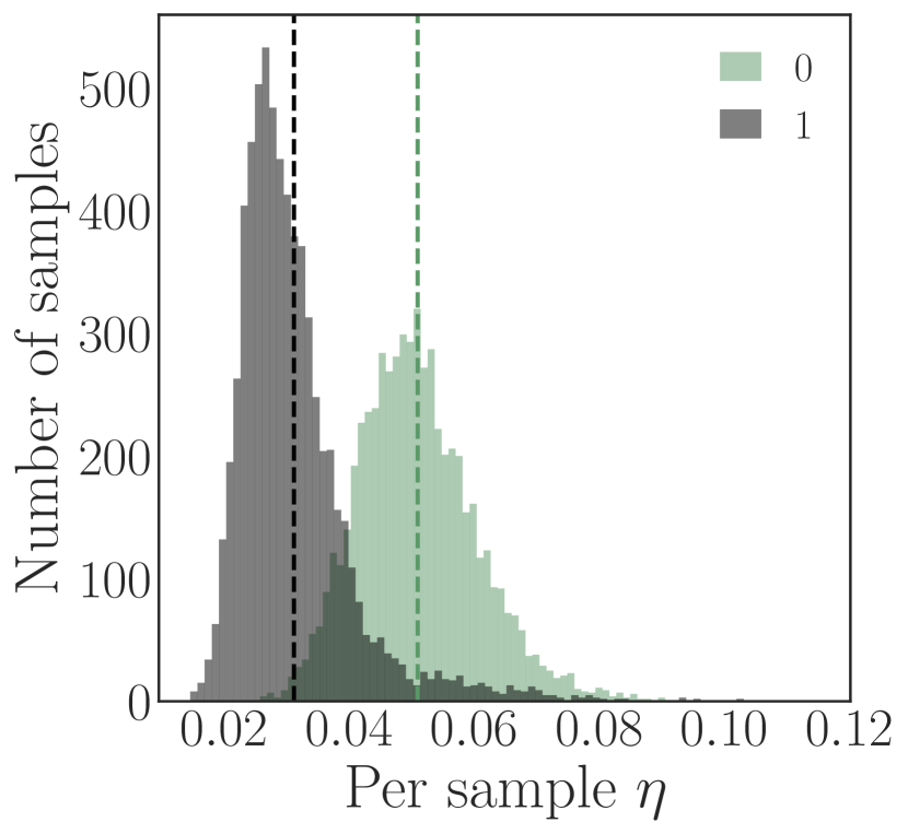
(a) Linear, MNIST

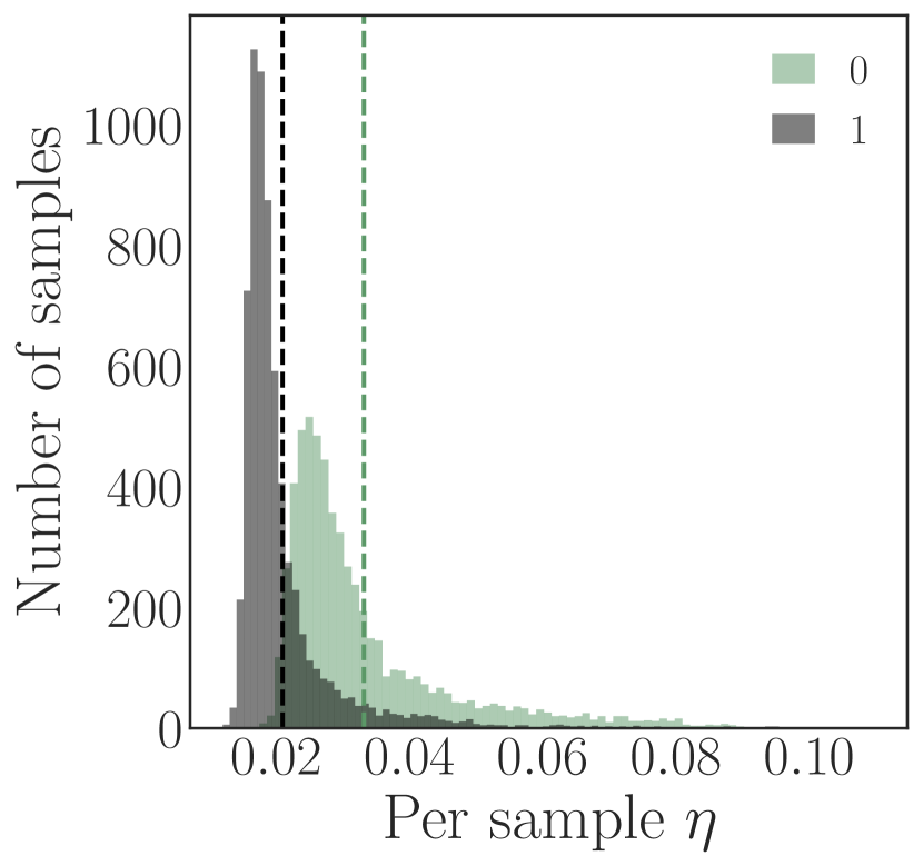
(b) Logistic, MNIST

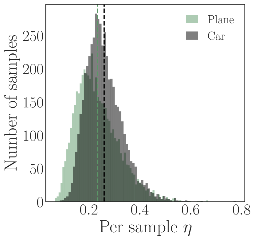
(c) Linear, CIFAR-10

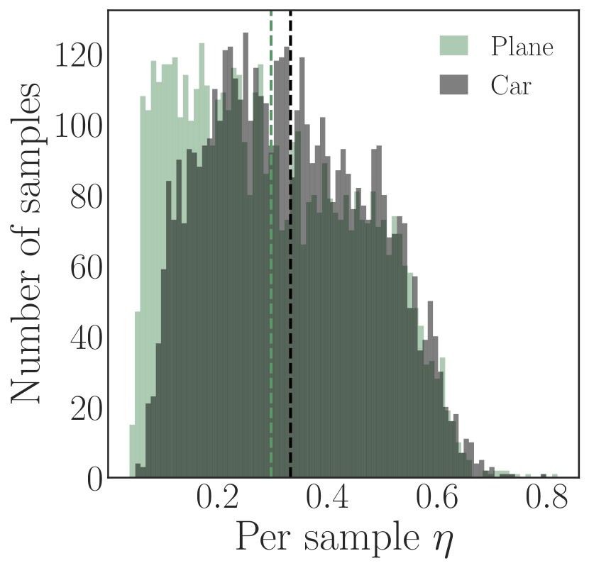
(d) Logistic, CIFAR-10

Figure 2: Histograms of per-example $\eta$ separated by class label for the MNIST and CIFAR-10 training sets for linear and logistic regression. Each class label’s mean $\eta$ is denoted by the dashed vertical line.

5 Iteratively Reweighted FIL

Prior work has shown that existing privacy mechanisms fail to provide equitable protection against privacy attacks for different subgroups [Yaghini et al., 2019]. We address this issue with iteratively reweighted Fisher information loss (IRFIL; Algorithm 1), which yields a model with an equal per-example FIL across all examples in ${\mathcal{D}}$. This is done by re-weighting the per-example surrogate loss $\ell({\bm{w}}^{\top}{\bm{x}}_{i},y_{i})$ over repeated computations of the minimizer ${\bm{w}}^{*}$.

After the first iteration in Algorithm 1, the weight for the $i$-th example is inversely proportional to the initial $\eta_{i}$. At successive iterations, the per-example weight $\omega_{i}^{t}$ is multiplicatively updated by a value inversely proportional to the current model’s FIL. The normalization on line 7 is primarily for numerical stability, keeping the weights from shrinking too rapidly. Without $L_{2}$ regularization, the resulting $\eta_{i}$ are invariant to the norm of the weights. With $L_{2}$ regularization, the normalization helps to keep the ratio of the primary objective to the regularization term constant.

If $\eta_{1}=\ldots=\eta_{n}=\eta$ are constant, then Algorithm 1 has converged since the update on line 7 yields a fixed point:

$$\omega_{i}^{t}=\frac{n\omega_{i}^{t-1}/\eta}{\sum_{i=1}^{n}\omega_{i}^{t-1}/\eta}=\frac{n\omega_{i}^{t-1}}{\sum_{i=1}^{n}\omega_{i}^{t-1}}=\frac{n\omega_{i}^{t-1}}{n}=\omega_{i}^{t-1},$$ (28)

where the second-to-last equality follows since the $\omega_{i}^{t-1}$ were normalized to sum to $n$ at the previous iteration.

Including the weights in computing ${\mathcal{I}}_{{\bm{w}}^{\prime}}({\bm{x}}_{i},y_{i})$ via equation 18 is a straightforward application of the chain rule:

$${\bm{J}}_{f_{i}}=-\omega_{i}\left(\textrm{diag}(\omega_{1},\ldots,\omega_{n}){\bm{H}}_{{\bm{w}}^{*}}\right)^{-1}\nabla_{{\bm{x}},y}\nabla_{\bm{w}}\ell.$$ (29)

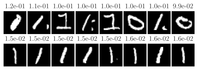
(a) Linear, MNIST

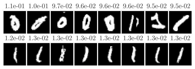
(b) Logistic, MNIST

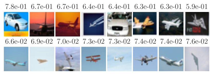
(c) Linear, CIFAR-10

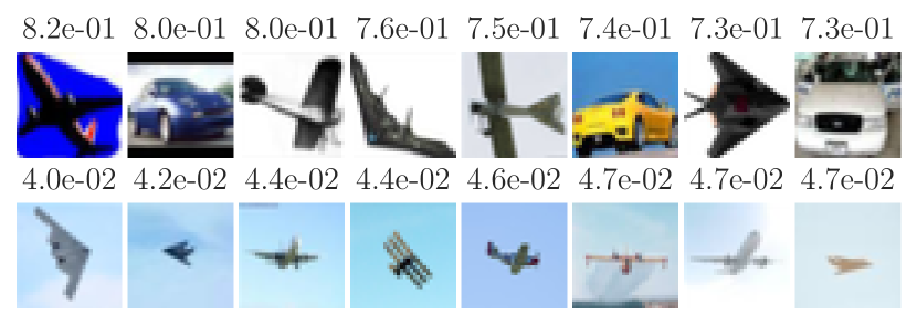
(d) Logistic, CIFAR-10

Figure 3: The eight images with the smallest and largest $\eta$ over the MNIST and CIFAR-10 training sets for linear and logistic regression. The number above each individual image is the corresponding $\eta$.

6 Experiments

We perform experiments with linear and logistic regression models on MNIST [LeCun and Cortes, 1998] and CIFAR-10 [Krizhevsky, 2009]. For attribute inversion attacks, we use the “IWPC" dataset from the Pharmacogenetics and Pharmacogenomics Knowledge Base [Klein et al., 2009] and the “Adult" dataset from the UC Irvine data repository [Dua and Graff, 2017]. Code to reproduce our results is available at https://github.com/facebookresearch/fisher_information_loss.

6.1 Experimental Setup

Datasets. On MNIST we perform binary classification of the digits $0$ and $1$ using a training dataset of 12,665 examples. On CIFAR-10, we classify images of planes from cars using a training dataset with 10,000 examples. We normalize all inputs to lie in the unit ball, $\max_{i}\|{\bm{x}}_{i}\|_{2}\leq 1$, and then project each input using PCA onto the top twenty principal components for the corresponding dataset.

The IWPC dataset requires estimating the stable dose of warfarin (an oral anticoagulant) based on clinical and genetic traits. We use the same preprocessed dataset as Yeom et al. [2018]. Of the 4,819 examples, we randomly split 20% into a test set and use the remaining 80% for the training set. The UCI Adult dataset requires classifying individuals with income above or below $50,000. We remove examples with missing features, leaving 30,162 examples in the training set and 15,060 in the test set. For the purpose of attribute inference, the marital status features are combined into a single category of married or unmarried and relationship features are removed [Mehnaz et al., 2020]. For both IWPC and UCI Adult, nominal features are converted to one-hot vectors with the last value dropped to avoid perfect collinearity in the encoding. Numerical features are centered to zero mean and unit variance. We do not otherwise preprocess the datasets, yielding a total of 14 features per example for IWPC and 86 features per example for UCI Adult.

Hyperparameters. Unless otherwise stated, for linear regression we do not apply $L_{2}$ regularization. For logistic regression, $\lambda$ is set to the largest value such that the training set accuracy is the same up to two significant digits as that of linear regression. For linear regression, the targets are $y_{i}\in\{-1,1\}$, and we compute the exact minimizer. For logistic regression, we use limited-memory BFGS to compute the minimizer. We typically report $\eta$ assuming a Gaussian noise scale of $\sigma=1$; hence $\eta=\|{\bm{J}}_{f}\|_{2}$.

6.2 Validating Fisher Information Loss

Histograms of the per-example $\eta$ for both MNIST and CIFAR-10 are shown in figure 2, separated by output class label. On MNIST the histograms have distinct modes. For both linear and logistic regression, the mode at the larger value is for the digit $0$, implying that the model in general contains more information about images of $0$ than of $1$. While the modes are not as distinct on CIFAR-10, the class-specific means are still separate, with class label “car" having a larger $\eta$ in general.

Figure 3 shows the eight images with the largest and smallest $\eta$ in each of the four settings. The images with the smallest $\eta$ are consistent with the class means in table 1. For MNIST, these correspond to the digit $1$ written in a very typical manner. For CIFAR-10, the smallest $\eta$ images are small planes on a blue-sky background. As expected, the images with the largest $\eta$ are much more idiosyncratic. Of the 100 largest $\eta$ examples for logistic and linear regression, 24 overlap for MNIST and 34 overlap for CIFAR-10.

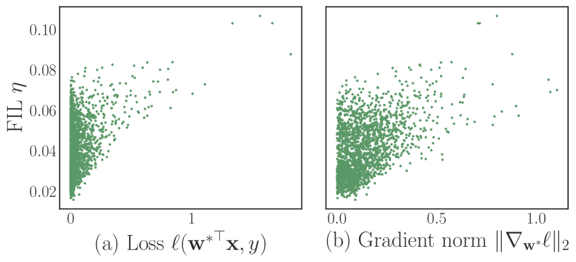
Figure 4: Scatter plots of the FIL $\eta$ with (a) the loss, and (b) the norm of the gradient on MNIST with linear regression and 2,000 randomly selected examples.

We compare $\eta$ to alternative heuristics that could correlate to the information a model contains about an example. Specifically, we measure the per-example loss $\ell({\bm{w}}^{*\top}{\bm{x}}_{i},y_{i})$, and the norm of the gradient $\|\nabla_{{\bm{w}}^{*}}\ell({\bm{w}}^{*\top}{\bm{x}}_{i},y_{i})\|_{2}$. Figure 4 shows scatter plots of $\eta$ against these alternatives. The FIL $\eta$ correlates with both metrics; however, high values of $\eta$ exist throughout the range of both alternatives. On the other hand, a low $\eta$ invariably implies a low loss. This shows that while loss-based heuristics may enjoy high precision in assessing privacy vulnerability, such heuristics should be used with caution, since they could suffer from low recall.

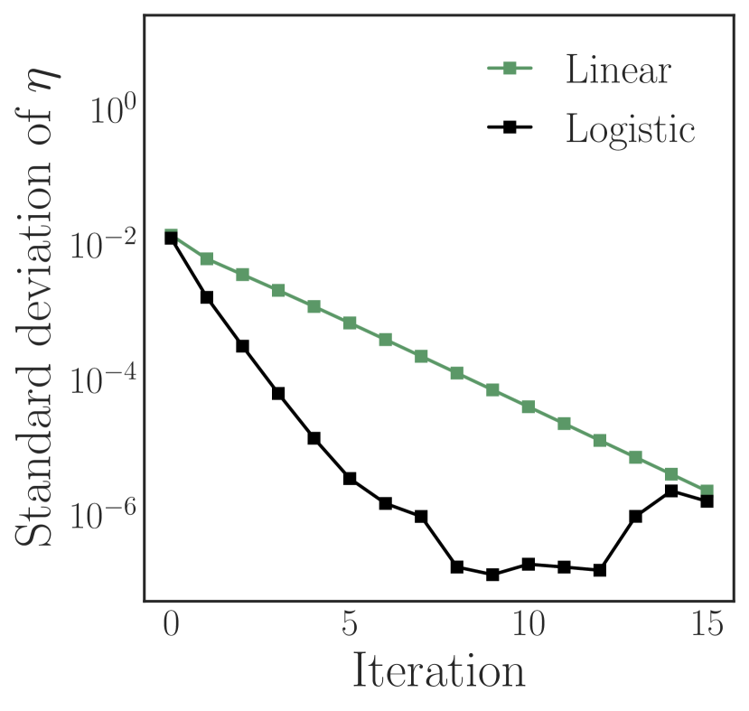
(a) MNIST

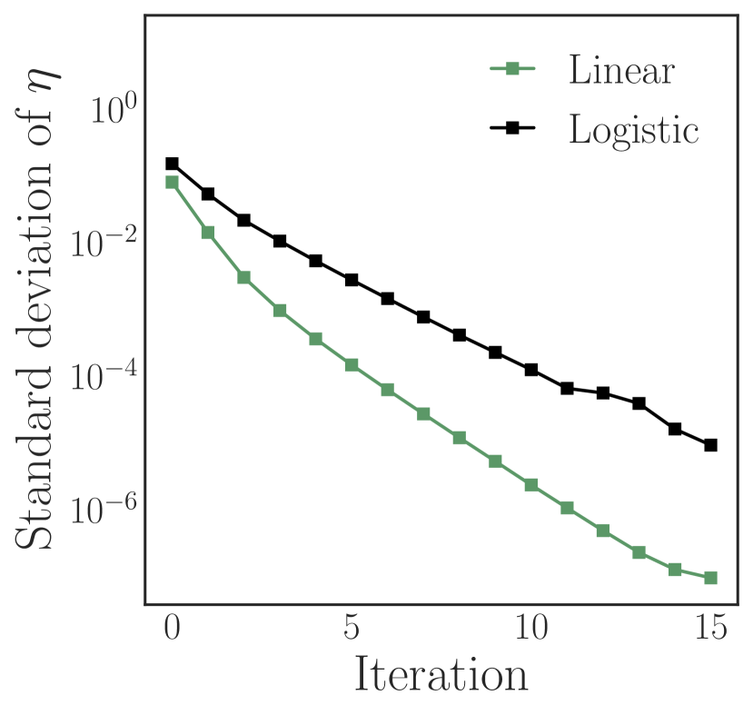
(b) CIFAR-10

Figure 5: The standard deviation of the example-level $\eta$ over iterations of the IRFIL algorithm.

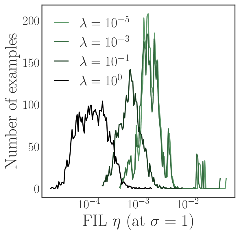
(a) Distribution of $\eta$

(b) Test MSE

(c) White-box attack

(d) Black-box attack

Figure 6: The effect of (a) the $L_{2}$ regularization parameter $\lambda$ on $\eta$ for IWPC, and the effect of the mean $\bar{\eta}$ varying $\lambda$ on (b) test MSE, (c) white-box accuracy, and (d) black-box accuracy. Standard deviations are computed over $100$ trials.

(a) IWPC; $\eta$ mean ($\pm$ SD)

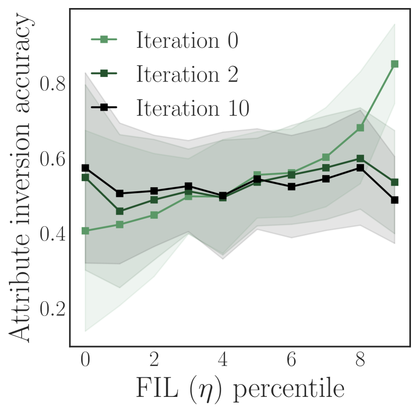
(b) IWPC; white-box accuracy

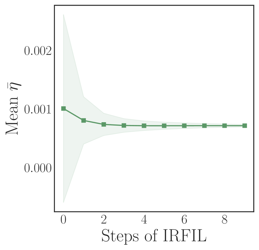
(c) UCI; mean $\bar{\eta}$ ($\pm$ SD)

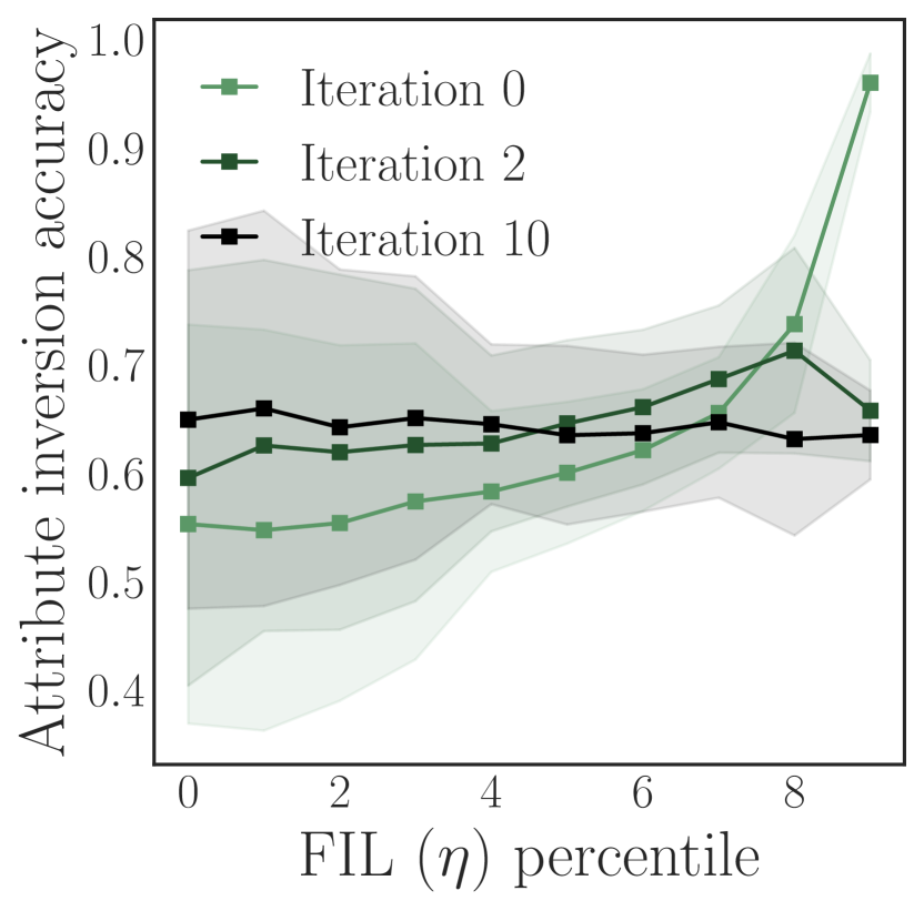
(d) UCI; white-box accuracy

Figure 7: We show how the per-example attribute-level $\eta$ converge over iterations of IRFIL for (a) IWPC and (c) UCI Adult. The mean accuracy of the white-box attack over increasing $\eta$-deciles also converges to a similar value over iterations of IRFIL for (b) IWPC and (d) UCI Adult. Standard deviations are computed over $100$ trials.

6.3 Reweighted FIL

We empirically evaluate the IRFIL algorithm in figure 5, which plots the standard deviation of the per-example $\eta$ against the number of re-weighting iterations. The per-example $\eta$ converge to the same value after only a few iterations for both linear and logistic regression on MNIST and CIFAR-10. Table 1 shows the mean and standard deviation of $\eta$, as well as the test accuracy for models trained with and without IRFIL. Neither the average FIL $\bar{\eta}$ nor the test accuracy are especially sensitive to the IRFIL algorithm. However, without IRFIL the standard deviation in $\eta$ is significantly higher, implying that the initial information leakage varies substantially across training examples. Overall, IRFIL achieves fairness in privacy loss with little change in accuracy or average privacy loss.

Table 1: The mean $\bar{\eta}$ ($\pm$ standard deviation) of the example-level $\eta$ and test accuracy before and after IRFIL.

	MNIST		CIFAR-10
Model	$\bar{\eta}$	Accuracy	$\bar{\eta}$	Accuracy
Linear	0.040 $\pm$ 0.014	100	0.26 $\pm$ 0.08	79.8
+IRFIL	0.047 $\pm$ 0.000	99.8	0.30 $\pm$ 0.00	80.7
Logistic	0.027 $\pm$ 0.012	99.8	0.32 $\pm$ 0.15	79.9
+IRFIL	0.024 $\pm$ 0.000	99.7	0.25 $\pm$ 0.00	79.1

6.4 Attribute Inference Attacks

We investigate how the success of attribute inference attacks varies with different levels of Fisher information loss. To do so, we use two attribute inversion attacks: 1) a white-box attack based on the FIL threat model, and 2) a black-box attack following the method described in Fredrikson et al. [2014]. The goal of the adversary is to infer the value of a nominal target attribute $x^{\textrm{tgt}}\in{\bm{x}}$ for a given example.

White-box attack. The white-box setting assumes the adversary has access to the complete training dataset ${\mathcal{D}}\setminus x_{i}^{\textrm{tgt}}$ for all but the target attribute of the example under attack. The adversary also has access to the perturbed model parameters ${\bm{w}}^{\prime}$. We also assume the adversary has complete knowledge of the model training details. Only the value of $x_{i}^{\textrm{tgt}}$ for the example under attack is opaque to the adversary.

The adversary infers the hidden attribute of the $i$-th example by estimating $\hat{x}_{i}^{\textrm{tgt}}$ to minimize the distance of the derived model from the given model ${\bm{w}}^{\prime}$:

$$\hat{x}_{i}^{\textrm{tgt}}=\operatorname*{arg\,min}_{x^{\textrm{tgt}}}\left\|{\bm{w}}^{\prime}-f({\mathcal{D}}\setminus x_{i}^{\textrm{tgt}}\cup x^{\textrm{tgt}})\right\|_{2},$$ (30)

where $f(\cdot)$ yields the minimizer (equation 13).

Black-box attack. In the black-box setting the adversary has access to the target example except the value of the target attribute ${\bm{x}}_{i}\setminus x_{i}^{\textrm{tgt}}$, the label $y_{i}$, the prior distribution $p(x^{\textrm{tgt}})$, model predictions $\phi({\bm{w}}^{\prime},{\bm{x}})$ via black-box queries, and model performance statistics $\pi(\phi({\bm{w}}^{\prime},{\bm{x}}),y)$. For a given model the attack infers the target attribute value by maximizing:

$$\hat{x}_{i}^{\textrm{tgt}}=\operatorname*{arg\,max}_{x^{\textrm{tgt}}}p(x^{\textrm{tgt}})\pi(\phi({\bm{w}}^{\prime},{\bm{x}}_{i}\setminus x_{i}^{\textrm{tgt}}\cup x^{\textrm{tgt}}),y_{i}).$$ (31)

We compare both attacks to a simple baseline adversary which infers the target attribute $\hat{x}_{i}^{\textrm{tgt}}=\operatorname*{arg\,max}_{x^{\textrm{tgt}}}p(x^{\textrm{tgt}})$.

For patients in IWPC, we infer the allele of the VKORC1 gene, which has three possible values. We use linear regression with $\lambda=10^{-2}$. For the black-box adversary, the performance metric $\pi(\phi({\bm{w}}^{\prime},{\bm{x}}),y)=p({\bm{w}}^{\prime\top}{\bm{x}};y,s^{2})$ is a Gaussian distribution with mean $y$ and variance given by the standard error $s^{2}$ on the training set.

Result. Figure 6 shows the effect of $L_{2}$ regularization and the mean $\bar{\eta}$ on the accuracy of the white-box and black-box attacks. For larger $\lambda$, the MSE degrades at smaller $\bar{\eta}$ (6(b)), suggesting more $L_{2}$ regularization requires less noise (smaller $\sigma$) to achieve the same $\bar{\eta}$. The white-box (6(c)) and black-box (6(d)) accuracies degrade as $\eta$ decreases. However, accross $\lambda$ the white-box accuracy follows $\bar{\eta}$ more closely than the black-box accuracy (6(d)), which tends to track with MSE. By choosing $\sigma$ such that $\bar{\eta}\approx 10^{-3}$, we can protect against both adversaries with little degradation in MSE.

We show the effect of IRFIL on the white-box attack using both the IWPC and UCI Adult datasets. For UCI Adult, we infer the binary marital status attribute. For both datasets, we compute $\eta$ specific to the attribute under attack for each example and use $\sigma=10^{-3}$. Figure 7 shows that the $\eta$ for each example rapidly converge to the same value over iterations of IRFIL. We sort the examples into deciles based on their initial $\eta$ values. We then compute the average attribute inversion accuracy for each decile at iterations of IRFIL. For both datasets, the highest $\eta$ decile is initially much more susceptible to attribute inversion than the lowest $\eta$ decile. However, after only two iterations of IRFIL, the inversion accuracies flatten substantially across $\eta$ deciles, and after ten iterations they are nearly constant. Hence, IRFIL can equalize vulnerability to privacy attacks across individuals.

7 Discussion and Future Work

We demonstrated that Fisher information loss can be used to assess the information leaked by a model about its training data. A primary benefit of FIL over a priori guarantees like differential privacy is the ability to measure information leakage at various granularities with respect to the data at hand. This also allows FIL to be used to construct models with equi-distributed leakage, which can be done with iteratively reweighted FIL. Furthermore, FIL explicitly measures the inferential power of an adversary, and we validated that it correctly captures vulnerability to privacy attacks. As a result, FIL can be used by practitioners to tailor the resulting privacy to the desired granularity and to the adversary’s knowledge and capabilities.

We motivated the use of FIL via the Cramér-Rao bound and delineated the corresponding threat model. However, the assumption that the adversary is limited to unbiased estimators may not hold in the presence of auxiliary information. The implications of this should be further investigated. Furthermore, unlike differential privacy, FIL does not implicitly degrade with correlated data. This property of FIL should also be further studied.

The IRFIL algorithm closely resembles iteratively reweighted least squares (IRLS), which has been widely studied for $\ell_{p}$-norm regression [Green, 1984, Burrus et al., 1994] and sparse recovery [Daubechies et al., 2010]. While IRLS often converges rapidly in practice, the theoretical convergence rates are difficult to derive and do not reflect the empirical results [Ene and Vladu, 2019]. We also observed rapid and robust convergence with the IRFIL algorithm without any hyper-parameter tuning. Future work may help understand the convergence of IRFIL from a theoretical standpoint.

Finally, we considered FIL in the common setting of output-perturbed generalized linear models with Gaussian noise. However, many possible extensions exist in the randomization used including alternative noise distributions such as the Laplace distribution [Dwork et al., 2006], objective perturbation [Chaudhuri et al., 2011], or quantifying leakage via predictions directly using, for example, the exponential mechanism [McSherry and Talwar, 2007]. Furthermore, extending FIL to the setting of non-linear and non-convex models will facilitate its utility and broader adoption.

Appendix A FISHER INFORMATION OF THE GAUSSIAN MECHANISM

We provide a simple derivation of the FIM of the Gaussian mechanism applied to the empirical risk minimizer, ${\bm{w}}^{*}$. The conditional probability density of the output perturbed parameters is given by:

$$p({\bm{w}}^{\prime}\mid{\mathcal{D}})=\int_{{\bm{w}}^{*}}p({\bm{w}}^{\prime}\mid{\bm{w}}^{*},{\mathcal{D}})p({\bm{w}}^{*}\mid{\mathcal{D}})d{\bm{w}}^{*}=p({\bm{w}}^{\prime}\mid{\bm{w}}^{*})$$ (32)

where in the last step we use the fact that ${\bm{w}}^{*}$ is sufficient for ${\bm{w}}^{\prime}$. We also assume $f({\mathcal{D}})$ is deterministic, and hence $p({\bm{w}}^{*}\mid{\mathcal{D}})$ is a (shifted) delta function nonzero at the optimal parameters, ${\bm{w}}^{*}$.

Using equation 32, the gradient of $\log p({\bm{w}}^{\prime}\mid{\mathcal{D}})$ with respect to ${\mathcal{D}}$ is given by:

$$\nabla_{{\mathcal{D}}}\log p({\bm{w}}^{\prime}\mid{\mathcal{D}})={\bm{J}}_{f}^{\top}\nabla_{{\bm{w}}^{*}}\log p({\bm{w}}^{\prime}\mid{\bm{w}}^{*})$$ (33)

where ${\bm{J}}_{f}$ is the Jacobian of $f({\mathcal{D}})$ with respect to ${\mathcal{D}}$. The Hessian is:

$$\begin{split}&\nabla^{2}_{\mathcal{D}}\log p({\bm{w}}^{\prime}\mid{\mathcal{D}})=\\ &{\bm{J}}_{f}^{\top}\nabla^{2}_{{\bm{w}}^{*}}\log p({\bm{w}}^{\prime}\mid{\bm{w}}^{*}){\bm{J}}_{f}+{\bm{\mathsfit{H}}}\nabla_{{\bm{w}}^{*}}\log p({\bm{w}}^{\prime}\mid{\bm{w}}^{*})\end{split}$$ (34)

where ${\bm{\mathsfit{H}}}$ is the three-dimensional tensor of second-order derivatives (in a slight abuse of notation ${\bm{\mathsfit{H}}}_{ijk}=\frac{\partial^{2}f_{k}}{\partial{\mathcal{D}}_{i}{\mathcal{D}}_{j}}$). Using the second-order expression for the FIM requires evaluating the expectation over ${\bm{w}}^{\prime}$ of equation 34.

When using zero-mean isotropic Gaussian noise for the perturbation, ${\mathcal{N}}(0,\sigma^{2}{\bm{I}})$, the expectation over ${\bm{w}}^{\prime}$ of equation 34 simplifies. The gradient of $\log p({\bm{w}}^{\prime}\mid{\bm{w}}^{*})$ is:

$$\nabla_{{\bm{w}}^{*}}\log p({\bm{w}}^{\prime}\mid{\bm{w}}^{*})=\frac{{\bm{w}}^{\prime}-{\bm{w}}^{*}}{\sigma^{2}},$$ (35)

and hence the Hessian is:

$$\nabla^{2}_{{\bm{w}}^{*}}\log p({\bm{w}}^{\prime}\mid{\bm{w}}^{*})=-\frac{1}{\sigma^{2}}{\bm{I}}.$$ (36)

Evaluating the expectation of equation 34 using the above expressions yields:

$$\mathbb{E}\left[{\bm{J}}_{f}^{\top}\nabla^{2}_{{\bm{w}}^{*}}\log p({\bm{w}}^{\prime}\mid{\bm{w}}^{*}){\bm{J}}_{f}+{\bm{\mathsfit{H}}}\nabla_{{\bm{w}}^{*}}\log p({\bm{w}}\mid{\bm{w}}^{*})\right]=$$

$${\bm{J}}_{f}^{\top}\mathbb{E}\left[\nabla^{2}_{{\bm{w}}^{*}}\log p({\bm{w}}^{\prime}\mid{\bm{w}}^{*})\right]{\bm{J}}_{f}+{\bm{\mathsfit{H}}}\mathbb{E}\left[\nabla_{{\bm{w}}^{*}}\log p({\bm{w}}^{\prime}\mid{\bm{w}}^{*})\right]=$$

$$-\frac{1}{\sigma^{2}}{\bm{J}}_{f}^{\top}{\bm{J}}_{f},$$

where the second term vanishes since $\mathbb{E}[{\bm{w}}^{\prime}]={\bm{w}}^{*}$. Hence the FIM is given by:

$${\mathcal{I}}_{{\bm{w}}^{\prime}}({\mathcal{D}})=-\mathbb{E}\left[\nabla^{2}_{\mathcal{D}}\log p({\bm{w}}^{\prime}\mid{\mathcal{D}})\right]=\frac{1}{\sigma^{2}}{\bm{J}}_{f}^{\top}{\bm{J}}_{f}.$$ (37)

Appendix B JACOBIAN OF THE MINIMIZER

Let $\ell({\bm{w}}^{\top}{\bm{x}},y)$ be a convex, twice-differentiable loss function. Let $f_{i}({\bm{x}},y)$ denote the minimizer of the regularized empirical risk as a function of $({\bm{x}},y)$ at the $i$-th example:

$$f_{i}({\bm{x}},y)=\operatorname*{arg\,min}_{{\bm{w}}}\sum_{j\neq i}\ell({\bm{w}}^{\top}{\bm{x}}_{j},y_{j})+\ell({\bm{w}}^{\top}{\bm{x}},y)+\frac{n\lambda}{2}\|{\bm{w}}\|_{2}^{2}.$$ (38)

We aim to derive an expression for ${\bm{J}}_{f_{i}}\big{\rvert}_{x_{i},y_{i}}$, the Jacobian of $f_{i}({\bm{x}},y)$ with respect to $({\bm{x}},y)$ evaluated at $({\bm{x}}_{i},y_{i})$. Taking the gradient of equation 38 with respect to ${\bm{w}}$ and setting it to $0$ gives an implicit function for ${\bm{w}}^{*}=f_{i}({\bm{x}},y)$:

$$0=\sum_{j\neq i}\nabla_{\bm{w}}\ell({\bm{w}}^{*\top}{\bm{x}}_{j},y_{j})+\nabla_{\bm{w}}\ell({\bm{w}}^{*\top}{\bm{x}},y)+n\lambda{\bm{w}}^{*}.$$ (39)

Implicit differentiation of equation 39 with respect to $({\bm{x}},y)$ gives:

$$0=\sum_{j\neq i}\nabla_{\bm{w}}^{2}\ell({\bm{w}}^{*\top}{\bm{x}}_{j},y_{j}){\bm{J}}_{f_{i}}+\nabla_{{\bm{x}},y}\nabla_{\bm{w}}\ell({\bm{w}}^{*\top}{\bm{x}},y)+n\lambda{\bm{J}}_{f_{i}}.$$ (40)

The second term can be computed using the product rule:

$$\nabla_{{\bm{x}},y} \nabla_{\bm{w}}\ell({\bm{w}}^{*\top}{\bm{x}},y)=$$

$$\nabla_{\bm{w}}^{2}\ell({\bm{w}}^{*\top}{\bm{x}},y){\bm{J}}_{f_{i}}+\nabla_{{\bm{x}},y}\nabla_{\bm{w}}\ell({\bm{w}}^{\top}{\bm{x}},y)\bigg{\rvert}_{{\bm{w}}={\bm{w}}^{*}}.$$ (41)

Evaluating equation 41 at $({\bm{x}}_{i},y_{i})$ and substituting into equation 40 yields:

$$0=$$

$$\left[\sum_{j=1}^{n}\nabla_{\bm{w}}^{2}\ell({\bm{w}}^{*\top}{\bm{x}}_{j},y_{j}){\bm{J}}_{f_{i}}+\nabla_{{\bm{x}},y}\nabla_{\bm{w}}\ell({\bm{w}}^{\top}{\bm{x}},y)+n\lambda{\bm{J}}_{f_{i}}\right]_{{\bm{w}}^{*},{\bm{x}}_{i},y_{i}}$$

$$=\bigg{[}{\bm{H}}_{{\bm{w}}^{*}}{\bm{J}}_{f_{i}}+\nabla_{{\bm{x}},y}\nabla_{\bm{w}}\ell({\bm{w}}^{\top}{\bm{x}},y)\bigg{]}_{{\bm{w}}^{*},{\bm{x}}_{i},y_{i}},$$ (42)

where the Hessian ${\bm{H}}_{{\bm{w}}^{*}}=\sum_{j=1}^{n}\nabla_{\bm{w}}^{2}\ell({\bm{w}}^{*\top}{\bm{x}}_{j},y_{j})+n\lambda{\bm{I}}$. Solving for ${\bm{J}}_{f_{i}}$ yields:

$${\bm{J}}_{f_{i}}\bigg{\rvert}_{{\bm{x}}_{i},y_{i}}=-{\bm{H}}_{{\bm{w}}^{*}}^{-1}\nabla_{{\bm{x}},y}\nabla_{\bm{w}}\ell({\bm{w}}^{*\top}{\bm{x}}_{i},y_{i}).$$ (43)