Higher order phase averaging for highly oscillatory systems

Abstract

We introduce a higher order phase averaging method for nonlinear oscillatory systems. Phase averaging is a technique to filter fast motions from the dynamics whilst still accounting for their effect on the slow dynamics. Phase averaging is useful for deriving reduced models that can be solved numerically with more efficiency, since larger timesteps can be taken. Recently, Haut and Wingate (2014) introduced the idea of computing finite window numerical phase averages in parallel as the basis for a coarse propagator for a parallel-in-time algorithm. In this contribution, we provide a framework for higher order phase averages that aims to better approximate the unaveraged system whilst still filtering fast motions. Whilst the basic phase average assumes that the solution is independent of changes of phase, the higher order method expands the phase dependency in a basis which the equations are projected onto. In this new framework, the original numerical phase averaging formulation arises as the lowest order version of this expansion in which the nonlinearity is projected onto the space of functions that are independent of the phase. Our new projection onto functions that are $k$th degree polynomials in the phase gives rise to higher order corrections to the phase averaging formulation. We illustrate the properties of this method on an ODE that describes the dynamics of a swinging spring due to Lynch (2002). Although idealized, this model shows an interesting analogy to geophysical flows as it exhibits a slow dynamics that arises through the resonance between fast oscillations. On this example, we show convergence to the non-averaged (exact) solution with increasing approximation order also for finite averaging windows. At zeroth order, our method coincides with a standard phase average, but at higher order it is more accurate in the sense that solutions of the phase averaged model track the solutions of the unaveraged equations more accurately.

Keywords: Phase averaging, slow-fast systems, resonant interactions

MSC 2020: 37M99

1 Introduction

One of the main challenges in simulating highly oscillatory multiscale PDEs is that the fast waves are known to create the lowest frequencies of the solution through nonlinear phase shifts, but are also responsible for severe linear wave time-step restrictions.

Phase averaging is a technique for approximating highly oscillatory systems so that the solution still captures the long time trends in the dynamics Sanders et al. (2007). In the context of highly oscillatory nonlinear PDEs, the combination of coordinate transformation, phase averaging, and asymptotics has been used to derive slow PDEs that do this (Schochet, 1994; Majda and Embid, 1998; Babin et al., 1997; Wingate et al., 2011, for example), providing rigorous derivations of slow geophysical models such as the quasigeostrophic model. Slow models are more analytically tractable and easier to explain, and they are more efficient to solve numerically. For an example numerical method inspired from the study of fast singular limits see (Jones et al., 1999). The reason they are more tractable to solve is because they have had the fast frequencies filtered from them, and therefore much larger timesteps can be taken without excessively compromising stability or accuracy. For example, the first numerical weather prediction exercise by Charney, Fjortoft and von Neumann (Charney et al., 1950) was based upon the barotropic vorticity equation, a model that does not support the full gravity and pressure waves present in more detailed models. One problem with asymptotic models is that they are only accurate at or near the limit, whereas the physically realistic parameters used in applications may not be near these limits, or the parameter regime itself may shift as the simulation unfolds. Ongoing research in theoretical fluid dynamics highlights an issue with using asymptotic equations that remove the fast oscillations: waves are responsible for transfering the energy toward the low frequencies, see (Smith and Waleffe, 2002). This is one reason asymptotic models are not used in contemporary weather and climate modeling as a predictive tool. In fact, the role of the oscillations has been found to be key to allowing accurate simulations and in some operational weather forcasting models, the compressible Euler equations, which include sound waves, are used; for many years sound waves were thought to be unimportant (Davies et al., 2003).

This paper is not about numerical algorithms, but it is highly motivated by them. Haut and Wingate (2014) investigated the possibility of using a framework inspired by the study of fast singular limits in that they use a coordinate transformation and phase averaging, but without asymptotics. Their goal was to use phase averaging to reduce high oscillations in the transformed solution, so that larger timesteps can be taken without triggering instability or producing large errors. They performed phase averaging over a finite window, and the phase average integral with numerical quadrature. Although this results in a computationally more intensive model, the terms in the quadrature sum can be evaluated independently, exposing possibilities for parallel computing. The phase averaged formulation also involves the application of matrix exponentials, which can be computed by Krylov methods or other techniques such as the parallel rational approximation approach of Haut et al. (2016); Caliari et al. (2021); Schreiber et al. (2018), particularly suited to oscillatory operators. This produces a variant of heterogeneous multiscale methods (Abdulle et al., 2012; Kevrekidis et al., 2003; Tao et al., 2010). The accuracy and stability of the finite window phase averaging technique was studied in Peddle et al. (2019), and applied to proving convergence of the parareal iteration. If the results of the averaging method are insufficiently accurate, then it can be used as the predictor in a predictor-corrector framework, see (Jones et al., 1999, for example). Many of these frameworks provide additional opportunities for parallel computing. With this in mind, Haut and Wingate (2014) introduced an asymptotic parareal method using the finite window averaging as a coarse propagator, and using a standard time integration method applied to the original unaveraged system as a fine propagator. This approach was extended to ODEs with nonlinear fast oscillations in Ariel et al. (2016).

In this paper we lay the foundations for an alternative approach to correcting averaging errors, where the accuracy of the finite window averaged model is increased “from the top down” by extending the phase average into a polynomial expansion of the solution in the phase variable. The goal is to further reduce the error in the slow component of the solution whilst still filtering fast oscillations. This increases the model complexity but it may be interesting to consider how to hide higher order corrections to the solution behind other computations in parallel, as occurs in the PFASST framework (Minion, 2011), for example. Here, we introduce and explore the higher order averaging technique applied to ODEs, although we have highly oscillatory PDEs and fast singular limits in mind when we do this. To isolate and understand the effects of our higher order averaging technique, in this paper we compute phase average integrals exactly (even though practical approaches would use numerical quadrature), and we use an adaptive timestepper to get a very accurate estimate of the ODE solution trajectory. We find that when applied to a swinging spring model introduced by Lynch (Holm and Lynch, 2002), the higher order averaging does indeed produce a more accurate solution than the basic finite window averaging, and that this error decreases as we increase the polynomial degree of the expansion in the phase variable.

The rest of the paper is organised as follows. In Section 2 we introduce the higher order averaging technique in the most general form, before specialising to a polynomial basis for the expansion in the phase variable as well as selecting a Gaussian averaging weight function so that the phase averaging can be computed analytically. This is not critical to the framework but was done to expediate our numerical experiments and to expose understanding of the effect of the higher order averaging. We then discuss asymptotic limits for the averaging window. In Section 3 we develop further formulae for Lynch’s swinging spring model, a specific low dimensional example. In Section 4 we present numerical integrations for the swinging spring example, calculating errors between the higher order average models and the exact model. Finally, in Section 5 we provide a summary and outlook.

2 Higher order averaging: formulation

We consider initial value problems written in the following abstract form

$$\frac{\partial}{\partial t}\mathbf{U}=L\mathbf{U}+N(\mathbf{U},\mathbf{U}),$$ (2.1)

where $L$ is a linear operator (with purely imaginary eigenvalues) and $N$ is a nonlinear operator. Restricting ourselves to quadratic nonlinearities, we assume $N$ to be a bilinear form (bilinearity indicated by the two slots). To develop phase averaged models, it is useful to reformulate (2.1) by introducing the factorization

$$\mathbf{V}(t)=e^{-tL}\mathbf{U}(t),$$ (2.2)

where the modulated variable $\mathbf{V}(t)$ satisfies the equation

$$\frac{\partial}{\partial t}\mathbf{V}(t)=e^{-tL}N\left(e^{tL}\mathbf{V}(t),e^{tL}\mathbf{V}(t)\right).$$ (2.3)

We refer to this form as the modulated equation. It is straightforward to show that both formulations are equivalent: when multiplying both sides of (2.1) with the integration factor $e^{-tL}$ and noting that $e^{-tL}(\partial_{t}\mathbf{U}-L\mathbf{U})=\partial_{t}(e^{-tL}\mathbf{U})$, we recover Eqn. (2.3) via

$$e^{-tL}(\partial_{t}\mathbf{U}-tL\mathbf{U})=e^{-tL}N(\mathbf{U},\mathbf{U}) \Leftrightarrow\partial_{t}(e^{-tL}\mathbf{U})=e^{-tL}N(\mathbf{U},\mathbf{U})$$ (2.4)

$$\Leftrightarrow\partial_{t}\mathbf{V}=e^{-tL}N(e^{tL}\mathbf{V},e^{tL}\mathbf{V}).$$ (2.5)

Note that this equation is valid for cases with or without scale separation (as discussed below).

To apply phase averaging, we add an additional phase parameter $s\in\mathbbm{R}$ over which we integrate and hence average the solution. As a first step, we assume a factorization

$$\mathbf{V}(t,s)=e^{-(t+s)L}\mathbf{U}(t)$$ (2.6)

where, besides the time parameter $t$, we include a phase parameter $s\in\mathbbm{R}$ in the exponent such that the solution in $\mathbf{V}$ depends on both $t$ and $s$. The phase parameter $s$ corresponds to a change in the point where the exponential $\exp((t+s)L)$ is equal to the identity, i.e. a phase shift.

As a calculation similar to above shows, this factorization yields a form of (2.3) that includes the parameter $s$, i.e.

$$\frac{\partial}{\partial t}\mathbf{V}(t,s)=e^{-(t+s)L}N\left(e^{(t+s)L}\mathbf{V}(t,s),e^{(t+s)L}\mathbf{V}(t,s)\right).$$ (2.7)

This gives us a one parameter family of solutions $\mathbf{V}(t,s)$ that depend on the phase parameter $s$ with the property that for $s=0$ we recover the solution of (2.3). We can then obtain a phase averaged model,

$$\frac{\partial}{\partial t}\bar{\mathbf{V}}(t)=\lim_{T\to\infty}\frac{1}{2T}\int_{-T}^{T}e^{-(t+s)L}N\left(e^{(t+s)L}\bar{\mathbf{V}}(t,s),e^{(t+s)L}\bar{\mathbf{V}}(t,s)\right)\operatorname{d}s.$$ (2.8)

Phase averaging for (2.7) was analysed by Schochet (1994) in the limit $\epsilon\to 0$, leading to slow equations that approximate the solution of the unaveraged model in this limit in some appropriate sense. In particular, Majda and Embid (1998) showed that this averaging and $\epsilon\to 0$ limit recovers the quasigeostrophic equation in the low Rossby number limit of the rotating shallow water equations, when written in this form. For finite Rossby number, Haut and Wingate (2014) proposed to adapt this approximation to numerical computations by keeping $T$ finite and introducing a $C^{\infty}$ weight function $\rho$ with $\rho\geq 0$, $\|\rho\|_{L^{1}}=1$, to obtain the averaged equation

$$\frac{\partial}{\partial t}\bar{\mathbf{V}}(t)=\int_{-\infty}^{\infty}\rho_{T}\left(s\right)e^{-(t+s)L}N\left(e^{(t+s)L}\bar{\mathbf{V}}(t,s),e^{(t+s)L}\bar{\mathbf{V}}(t,s)\right)\operatorname{d}s,$$ (2.9)

where $\rho_{T}(s)=\rho(s/T)/T$. They further proposed to replace the integral via quadrature (choosing $\rho$ to have compact support), with the evaluation of the integrand at each quadrature point being computed independently in parallel; this formulation provided the coarse propagator for a parallel-in-time algorithm. The reason for the phase averaging in that paper, and this one, is to remove high oscillations from the modulated variable, allowing larger timesteps to be taken in a numerical solver. This averaging introduces an error in the solution, and the goal of this paper is to introduce refinements to the phase averaging procedure so that this error can be reduced.

Note that depending on the value of $T$, formulation (2.9) recovers an averaged version, an asymptotic approximation, or the full equations (2.3):

• for $T\rightarrow 0$, we recover Eqn. (2.3) because in the limit $T\rightarrow 0$ the weight function $\rho$ converges formally to the Dirac measure $\delta(s)$.

• for $T\rightarrow\infty$, we recover (2.9), because when integrating the resulting integral value is invariant under shifts in $t$; hence for $t=0$ we recover the asymptotic approximation introduced in Majda and Embid (1998) after also taking $\epsilon\to 0$.

• for $0<<T<<\infty$, formulation (2.9) has a smoothing effect on fast oscillations with time period less than $T$.

The optimum choice of $T$ as a function of $\epsilon$ to minimise the error due to averaging when combined with a numerical time integration method to solve (2.9) was investigated in Peddle et al. (2019).

An interpretation of (2.9) is that we have projected $\mathbf{V}(t,s)$ onto the space of functions independent of $s$ using the $\rho$-weighted $L^{2}$ inner product. In the next subsection, our higher order averaging method for finite averaging window $T$ will be based on projecting the one parameter family of solutions on to higher order polynomials in $s$. After solving this system of coupled differential equations, we set $s=0$ because we are interested only in the time evolution of the solution with this phase value. Hence, we only present solutions at $s=0$ in the numerical results section.

2.1 General framework of higher order time averaging

We abbreviate the RHS of (2.3) as general bilinear function $\mathbf{F}(\mathbf{V}(t,s),\mathbf{V}(t,s);t+s)$ that has quadratic dependency on $\mathbf{V}(t,s)$, i.e.

$$\frac{\partial}{\partial t}\mathbf{V}(t,s)=\mathbf{F}\big{(}\mathbf{V}(t,s),\mathbf{V}(t,s);t+s\big{)}.$$ (2.10)

According to (2.6), the solution vector $\mathbf{V}$ depends on both $t$ and $s$ and we make the approximation that it can be represented by the factorization

$$\mathbf{V}(t,s)=\sum_{k=0}^{p}\mathbf{V}_{k}(t)\phi_{k}(s),$$ (2.11)

where $\phi_{k}(s)$ are basis vectors depending on $s$ that span $Q$, some chosen $(p+1)$-dimensional function space.

We project (2.10) onto $Q$ to obtain

$$\int_{-\infty}^{\infty}\rho_{T}\left({s}\right)\mathbf{W}(s)\cdot\frac{\partial}{\partial t}\mathbf{V}(t,s)ds=\int_{-\infty}^{\infty}\rho_{T}\left({s}\right)\mathbf{W}(s)\cdot\mathbf{F}\big{(}\mathbf{V}(t,s),\mathbf{V}(t,s);t+s\big{)}ds\quad\forall\mathbf{W}(s)\in Q,$$ (2.12)

where $\rho_{T}(s)=\rho(s/T)/T$ for our chosen weight function $\rho$.

Also expanding the test function $\mathbf{W}$ in the basis,

$$\mathbf{W}(s)=\sum_{j=0}^{p}\mathbf{W}_{j}\phi_{j}(s),$$ (2.13)

we get

$$\begin{split}\sum_{j=0}^{p}\sum_{k=0}^{p}&\mathbf{W}_{j}\int_{-\infty}^{\infty}\frac{1}{T}\rho\left(\frac{s}{T}\right){\phi_{j}(s)\phi_{k}(s)ds}\frac{\partial}{\partial t}\mathbf{V}_{k}(t)=\\ &\sum_{j=0}^{p}\mathbf{W}_{j}\int_{-\infty}^{\infty}\frac{1}{T}\rho\left(\frac{s}{T}\right)\phi_{j}(s)\mathbf{F}\big{(}\sum_{k=0}^{p}\mathbf{V}_{k}(t)\phi_{k}(s),\sum_{l=0}^{p}\mathbf{V}_{l}(t)\phi_{l}(s);t+s\big{)}ds,\quad\forall\,\mathbf{W}_{1},\ldots,\mathbf{W}_{p}.\end{split}$$ (2.14)

As the coefficients $\mathbf{W}_{j}$ are independent from each other, we obtain

$$\begin{split}\sum_{k=0}^{p}\int_{-\infty}^{\infty}\frac{1}{T}\rho\left(\frac{s}{T}\right)&{\phi_{j}(s)\phi_{k}(s)ds}\frac{\partial}{\partial t}\mathbf{V}_{k}(t)=\\ &\int_{-\infty}^{\infty}\frac{1}{T}\rho\left(\frac{s}{T}\right)\phi_{j}(s)\mathbf{F}\big{(}\sum_{k=0}^{p}\mathbf{V}_{k}(t)\phi_{k}(s),\sum_{l=0}^{p}\mathbf{V}_{l}(t)\phi_{l}(s);t+s\big{)}ds.\end{split}$$ (2.15)

This defines our averaged model for the components $\mathbf{V}_{k}$, in the form of a matrix-vector equation for $\frac{\partial}{\partial t}\mathbf{V}_{k}$. To use it, we set $\mathbf{V}(t=0,s)=\mathbf{U}(0)$, the initial condition, independently of $s$. Then we solve the equations forward in time (perhaps approximating the phase integral as a sum), taking the solutions at $s=0$.

To understand more about what this approximation does, we further specify the nonlinear function $\mathbf{F}$. As it is bilinear, we may pull out the double sum over the basis $\phi$, i.e.

$$\begin{split}\mathbf{F}\left(\sum_{k=0}^{p}\mathbf{V}_{k}(t)\phi_{k}(s),\sum_{l=0}^{p}\mathbf{V}_{l}(t)\phi_{l}(s);t+s\right)=&\sum_{k=0}^{p}\sum_{l=0}^{p}\phi_{k}(s)\phi_{l}(s)\mathbf{F}\big{(}\mathbf{V}_{k}(t),\mathbf{V}_{l}(t);t+s\big{)}.\end{split}$$ (2.16)

Moreover, we assume that we can factor out the time dependency of $\mathbf{F}$ on $t+s$ so that $\mathbf{F}$ is represented as

$$\mathbf{F}\big{(}\mathbf{V}_{k}(t),\mathbf{V}_{l}(t);t+s\big{)}=\sum_{m}\mathbf{F}_{m}\big{(}\mathbf{V}_{k}(t),\mathbf{V}_{l}(t)\big{)}e^{i{(t+s)c_{m}}}$$ (2.17)

where the sum in $m$ is over different terms that are quadratic in $\mathbf{V}$ (for different polynomial order $k,l$) with coefficients $c_{m}$ and bilinear functions $\mathbf{F}_{m}$ and that depend on the nonlinear operator $N$. In the case of a PDE, this sum over $m$ will be replaced by an infinite sum over frequencies. Examples of these coefficients and their relations are shown further below in Table 3.1 for the swinging spring model. To ease notation, we will adopt the short hand notation $\mathbf{F}_{m,k,l}(t):=\mathbf{F}_{m}\big{(}\mathbf{V}_{k}(t),\mathbf{V}_{l}(t)\big{)}$.

In summary, we end up with a system of equations (for $j=0,\dots p$) that reads

$$\begin{split}\sum_{k=0}^{p}&\int_{-\infty}^{\infty}\frac{1}{T}\rho\left(\frac{s}{T}\right){\phi_{j}(s)\phi_{k}(s)ds}\frac{\partial}{\partial t}\mathbf{V}_{k}(t)=\\ &\sum_{m}\sum_{k=0}^{p}\sum_{l=0}^{p}\mathbf{F}_{m,k,l}(t)\int_{-\infty}^{\infty}\frac{1}{T}\rho\left(\frac{s}{T}\right)\phi_{j}(s)\phi_{k}(s)\phi_{l}(s)e^{i{(t+s)c_{m}}}ds\quad\forall\phi_{j}(s).\end{split}$$ (2.18)

This formulation provides a general framework of higher order averages for various choices of $Q$ and weight function $\rho$.

2.2 Polynomial higher order time averaging

In this section we make some specific calculations using the choice of $Q=P_{p}$, the degree-p polynomials, and a particular choice of weight function that allows us to make progress analytically, namely $\rho(s)=\exp(-s^{2}/2)/\sqrt{2\pi}$, recalling that

$$\int_{-\infty}^{\infty}\frac{1}{T}\rho\left(\frac{s}{T}\right)ds=\int_{-\infty}^{\infty}\frac{1}{\sqrt{2\pi T^{2}}}e^{-\frac{s^{2}}{2T^{2}}}ds=1.$$ (2.19)

This allows us to integrate over the whole $\mathbbm{R}$ while guaranteeing a bounded integral, but other choices are possible too.

As a basis $\phi$, we choose the standard monomials

$$\phi_{j}(s)=s^{j},\quad j=0,\dots,p.$$ (2.20)

This is a poorly-conditioned basis, and better choices might be made for large values of $p$ (for the weight function we are using the Hermite polynomials would be ideal since they diagonalise the mass matrix). However, the monomial basis simplifies the calculations below. Also, under this basis, ${\mathbf{V}}(t,s=0)={\mathbf{V}}_{0}(t)$, so to initialise the system we can just set ${\mathbf{V}}_{0}(0)=\mathbf{V}(0,s=0)$ and ${\mathbf{V}}_{k}(0)=0$ for $1\leq k\leq p$.

Substituting this basis into (2.18), we arrive at

$$\begin{split}\sum_{k=0}^{p}&\frac{1}{\sqrt{2\pi T^{2}}}\int_{-\infty}^{\infty}e^{-\frac{s^{2}}{2T^{2}}}{s^{j}s^{k}ds}\frac{\partial}{\partial t}\mathbf{V}_{k}(t)=\\ &\sum_{m}\sum_{k=0}^{p}\sum_{l=0}^{p}\mathbf{F}_{m,k,l}(t)e^{ic_{m}t}\frac{1}{\sqrt{2\pi T^{2}}}\int_{-\infty}^{\infty}e^{-\frac{s^{2}}{2T^{2}}}e^{i{c_{m}}s}s^{j}s^{k}s^{l}ds\quad\forall j.\end{split}$$ (2.21)

The latter equation can be formulated more concisely as

$$\begin{split}\sum_{k=0}^{p}\mathrm{M}_{jk}\frac{\partial}{\partial t}\mathbf{V}_{k}(t)=\sum_{m}\sum_{k=0}^{p}\sum_{l=0}^{p}\mathbf{F}_{m,k,l}(t)e^{i{c_{m}}t}\tilde{\mathrm{R}}_{jkl}^{m}\quad\forall j,\end{split}$$ (2.22)

in which we denote the integral on the left hand side (LHS) of (2.21) as a mass matrix

$$\mathrm{M}_{jk}=\frac{1}{\sqrt{2\pi T^{2}}}\int_{-\infty}^{\infty}e^{-\frac{s^{2}}{2T^{2}}}{s^{j}s^{k}ds},$$ (2.23)

and that on the RHS of (2.21) as

$$\tilde{\mathrm{R}}_{jkl}^{m}=\frac{1}{\sqrt{2\pi T^{2}}}\int_{-\infty}^{\infty}e^{-\frac{s^{2}}{2T^{2}}}e^{i{c_{m}}s}s^{j}s^{k}s^{l}ds.$$ (2.24)

To evaluate these integrals, it will be useful to introduce the notation

$$I_{\alpha}:=\frac{1}{\sqrt{2\pi T^{2}}}\int_{-\infty}^{\infty}e^{-\frac{s^{2}}{2T^{2}}}{s^{\alpha}ds}$$ (2.25)

with $I_{0}=1$ which follows immediately from (2.19). Then, for instance, for $\alpha=i+j$ we have $M_{ij}=I_{\alpha}$. With the help of this concise notation, we formulate the following two propositions that allow us to evaluate the integrals in (2.23) and (2.24).

Proposition 2.1.

For averaging window $T$ and $\alpha=j+k$ with $j,k=0,\dots,p$, the integral $I_{\alpha}$ in (2.25) can be represented in the recursive form

$$I_{\alpha}=T^{2}(\alpha-1)I_{\alpha-2}\quad\text{with}\quad I_{0}=1$$ (2.26)

In particular, $I_{\alpha}=0$ for all $\alpha$ odd.

Proof.

This recursive formula follows directly from integration by parts. Using the normalization factor $\gamma=\frac{1}{\sqrt{2\pi T^{2}}}$, there follows

$$\begin{split}I_{\alpha}=\gamma\int_{-\infty}^{\infty}\frac{d}{ds}e^{-\frac{s^{2}}{2T^{2}}}\frac{-2T^{2}}{2s}s^{\alpha}ds&=\gamma\left[-e^{-\frac{s^{2}}{2T^{2}}}T^{2}s^{\alpha-1}\right]_{-\infty}^{\infty}+T^{2}(\alpha-1)\gamma\int_{-\infty}^{\infty}e^{-\frac{s^{2}}{2T^{2}}}s^{\alpha-2}ds\\ &=T^{2}(\alpha-1)I_{\alpha-2}.\end{split}$$ (2.27)

For $\alpha=0$, we have $I_{0}=1$ since $\int_{-\infty}^{\infty}e^{-\frac{s^{2}}{2T^{2}}}=\sqrt{2\pi T^{2}}$ which follows from (2.19). For odd $\alpha$, $I_{\alpha}$ is an integral of a product of an even and odd function over entire $\mathbbm{R}$, hence zero. ∎

Proposition 2.2.

Using the recursive formula of Proposition 2.1 and for averaging window $T$ and $\alpha=j+k+l$ with $j,k,l=0,\dots,p$, the integral (2.24) can be represented for all $m$ as

$$\tilde{\mathrm{R}}_{\alpha}^{m}=e^{-\frac{c_{m}^{2}T^{2}}{2}}\mathrm{R}_{\alpha}^{m}\quad\text{with}\quad\mathrm{R}^{m}_{\alpha}=\sum_{\beta=0}^{\alpha}\binom{\alpha}{\beta}I_{\alpha-\beta}\cdot(ic_{m}T^{2})^{\beta}$$ (2.28)

with the property that for $\alpha=0$ we have $\mathrm{R}^{m}_{0}=1$ for all $m$.

Proof.

First, we rewrite (2.24) using $\alpha=j+k+l$ and by completing the square ($-\frac{s^{2}}{2T^{2}}+ic_{m}s=-\frac{1}{2T^{2}}(s-ic_{m}T^{2})^{2}-\frac{c_{m}^{2}T^{2}}{2}$) we arrive at

$$\tilde{\mathrm{R}}_{\alpha}^{m}=e^{-\frac{c_{m}^{2}T^{2}}{2}}\mathrm{R}_{\alpha}^{m}\quad\text{with}\quad\mathrm{R}_{\alpha}^{m}:=\frac{1}{\sqrt{2\pi T^{2}}}\int_{-\infty}^{\infty}e^{-\frac{1}{2T^{2}}(s-ic_{m}T^{2})^{2}}s^{\alpha}ds.$$ (2.29)

Next, we use the substitution $s^{\prime}=s-ic_{m}T^{2}$ with $ds^{\prime}=ds$:

$$\mathrm{R}_{\alpha}^{m}=\frac{1}{\sqrt{2\pi T^{2}}}\int_{-\infty-ic_{m}T^{2}}^{\infty-ic_{m}T^{2}}e^{-\frac{s^{\prime 2}}{2T^{2}}}(s^{\prime}+ic_{m}T^{2})^{\alpha}ds^{\prime}.$$ (2.30)

Because the latter is a contour integral in the complex domain in which one term is integrated along the real axis and another one along a semi circle at infinity, the shift of the real axis in the complex direction by $-ic_{m}T^{2}$ does not change the integral value as long as there are no, or the same number of singularities enclosed by the contour. Therefore, we can equivalently write

$$\mathrm{R}_{\alpha}^{m}=\frac{1}{\sqrt{2\pi T^{2}}}\int_{-\infty}^{\infty}e^{-\frac{s^{\prime 2}}{2T^{2}}}(s^{\prime}+ic_{m}T^{2})^{\alpha}ds^{\prime}$$ (2.31)

while for $\alpha=0$ there follows

$$\mathrm{R}_{0}^{m}={\frac{1}{\sqrt{2\pi T^{2}}}\int_{-\infty-ic_{m}T^{2}}^{\infty-ic_{m}T^{2}}e^{-\frac{s^{\prime 2}}{2T^{2}}}ds^{\prime}}={\frac{1}{\sqrt{2\pi T^{2}}}\int_{-\infty}^{\infty}e^{-\frac{s^{\prime 2}}{2T^{2}}}ds^{\prime}}=1.$$ (2.32)

For the ease of notation, we will skip ^′ in the following. Using the binomial expansion $(x+y)^{\alpha}=\sum_{\beta=0}^{\alpha}\binom{\alpha}{\beta}x^{\alpha-\beta}y^{\beta}$, Eqn. (2.31) becomes

$$\mathrm{R}^{m}_{\alpha}=\sum_{\beta=0}^{\alpha}\binom{\alpha}{\beta}\left(\frac{1}{\sqrt{2\pi T^{2}}}\int_{-\infty}^{\infty}e^{\frac{-s^{2}}{2T^{2}}}s^{\alpha-\beta}ds\right)(ic_{m}T^{2})^{\beta}.$$ (2.33)

The statement follows by using expression (2.26) for the term in brackets. ∎

Based on these results, we can further expand (2.22) to get

$$\begin{split}\sum_{k=0}^{p}\mathrm{M}_{jk}\frac{\partial}{\partial t}\mathbf{V}_{k}(t)=\sum_{m}\sum_{k=0}^{p}\sum_{l=0}^{p}\mathbf{F}_{m,k,l}(t)\mathrm{R}_{jkl}^{m}e^{ic_{m}t}e^{-\frac{c_{m}^{2}T^{2}}{2}}\quad\text{for}\quad j=0,1,2,\end{split}$$ (2.34)

where $\mathrm{M}_{jk}=\mathrm{M}_{\alpha}$ for $\alpha=j+k$ and $\mathrm{R}_{jkl}^{m}=\mathrm{R}^{m}_{\alpha}$ for $\alpha=j+k+l$. Note that $\mathbf{F}_{m,k,l}=\mathbf{F}_{m,l,k}$ for all $m,k,l$.

Equation (2.34) will serve us in Section 3 to develop a higher order averaging method for an ODE describing a swinging spring. But before we discuss this example, let us first present an explicit representation of (2.34) and how the equation behaves in the zero and infinity limits of $T$.

2.2.1 Explicit representation for polynomial order $p=2$

For the sake of clarity, we present an explicit representation of Eqn. (2.34) for $p=2$, i.e. $j,k,l=0,1,2$. Proposition 2.1 leads to a mass matrix $\mathrm{M}$ with coefficients (in terms of $\mathrm{M}_{\alpha}$):

$$\mathrm{M}_{0}=1,\quad\mathrm{M}_{1}=0,\quad\mathrm{M}_{2}=T^{2},\quad\mathrm{M}_{3}=0,\quad\mathrm{M}_{4}=3T^{4};$$ (2.35)

and we can explicitly write the inverse of $\mathrm{M}$ as

$$\mathrm{M}^{-1}=\begin{pmatrix}1&0&T^{2}\\ 0&T^{2}&0\\ T^{2}&0&3T^{4}\\ \end{pmatrix}^{-1}=\begin{pmatrix}\frac{3}{2}&0&\frac{-1}{2T^{2}}\\ 0&\frac{1}{T^{2}}&0\\ \frac{-1}{2T^{2}}&0&\frac{1}{2T^{4}}\\ \end{pmatrix}.$$ (2.36)

Moreover, Proposition 2.2 leads to the coefficients (in terms of $\mathrm{R}^{m}_{\alpha}$):

$$\begin{split}&\mathrm{R}_{0}^{m}=1,\quad\mathrm{R}_{1}^{m}=ic_{m}T^{2},\quad\mathrm{R}_{2}^{m}=T^{2}-c_{m}^{2}T^{4},\quad\mathrm{R}_{3}^{m}=i3c_{m}T^{4}-ic_{m}^{3}T^{6},\\ &\mathrm{R}_{4}^{m}=3T^{4}-6c_{m}^{2}T^{6}+c_{m}^{4}T^{8},\quad\mathrm{R}_{5}^{m}=i15cmT^{6}-i10c_{m}^{3}T^{8}+ic_{m}^{5}T^{10},\\ &\mathrm{R}_{6}^{m}=15T^{6}-45c_{m}^{2}T^{8}+15c_{m}^{4}T^{10}-c_{m}^{6}T^{12}.\end{split}$$ (2.37)

With these coefficients, the explicit form of Eqn. (2.34) reads

$$\begin{split}&\begin{pmatrix}M_{00}&0&M_{02}\\ 0&M_{11}&0\\ M_{20}&0&M_{22}\\ \end{pmatrix}\begin{pmatrix}\dot{\mathbf{V}}_{0}(t)\\ \dot{\mathbf{V}}_{1}(t)\\ \dot{\mathbf{V}}_{2}(t)\\ \end{pmatrix}=\sum_{m}\sum_{k=0}^{2}\sum_{l=0}^{2}e^{ic_{m}t}e^{-\frac{c_{m}^{2}T^{2}}{2}}\mathbf{F}_{m,k,l}\begin{pmatrix}\mathrm{R}_{0kl}^{m}\\ \mathrm{R}_{1kl}^{m}\\ \mathrm{R}_{2kl}^{m}\\ \end{pmatrix}\\ &=\sum_{m}e^{ic_{m}t}e^{-\frac{c_{m}^{2}T^{2}}{2}}\times\Big{[}\mathbf{F}_{m,0,0}\begin{pmatrix}\mathrm{R}_{000}^{m}\\ \mathrm{R}_{100}^{m}\\ \mathrm{R}_{200}^{m}\\ \end{pmatrix}+\mathbf{F}_{m,0,1}\begin{pmatrix}\mathrm{R}_{001}^{m}\\ \mathrm{R}_{101}^{m}\\ \mathrm{R}_{201}^{m}\\ \end{pmatrix}+\mathbf{F}_{m,0,2}\begin{pmatrix}\mathrm{R}_{002}^{m}\\ \mathrm{R}_{102}^{m}\\ \mathrm{R}_{202}^{m}\\ \end{pmatrix}+\mathbf{F}_{m,1,0}\begin{pmatrix}\mathrm{R}_{010}^{m}\\ \mathrm{R}_{110}^{m}\\ \mathrm{R}_{210}^{m}\\ \end{pmatrix}\\ &+\mathbf{F}_{m,1,1}\begin{pmatrix}\mathrm{R}_{011}^{m}\\ \mathrm{R}_{111}^{m}\\ \mathrm{R}_{211}^{m}\\ \end{pmatrix}+\mathbf{F}_{m,1,2}\begin{pmatrix}\mathrm{R}_{012}^{m}\\ \mathrm{R}_{112}^{m}\\ \mathrm{R}_{212}^{m}\\ \end{pmatrix}+\mathbf{F}_{m,2,0}\begin{pmatrix}\mathrm{R}_{020}^{m}\\ \mathrm{R}_{120}^{m}\\ \mathrm{R}_{220}^{m}\\ \end{pmatrix}+\mathbf{F}_{m,2,1}\begin{pmatrix}\mathrm{R}_{021}^{m}\\ \mathrm{R}_{121}^{m}\\ \mathrm{R}_{221}^{m}\\ \end{pmatrix}+\mathbf{F}_{m,2,2}\begin{pmatrix}\mathrm{R}_{022}^{m}\\ \mathrm{R}_{122}^{m}\\ \mathrm{R}_{222}^{m}\\ \end{pmatrix}\Big{]}.\end{split}$$ (2.38)

Bringing $\mathrm{M}$ to the LHS, we result in

$$\begin{split}\begin{pmatrix}\dot{\mathbf{V}}_{0}(t)\\ \dot{\mathbf{V}}_{1}(t)\\ \dot{\mathbf{V}}_{2}(t)\\ \end{pmatrix}=\sum_{m}\sum_{k=0}^{2}\sum_{l=0}^{2}e^{ic_{m}t}e^{-\frac{c_{m}^{2}T^{2}}{2}}\mathbf{F}_{m,k,l}\left(\begin{pmatrix}\frac{3}{2}\\ 0\\ \frac{-1}{2T^{2}}\\ \end{pmatrix}\mathrm{R}_{0kl}^{m}+\begin{pmatrix}0\\ \frac{1}{T^{2}}\\ 0\\ \end{pmatrix}\mathrm{R}_{1kl}^{m}+\begin{pmatrix}\frac{-1}{2T^{2}}\\ 0\\ \frac{1}{2T^{4}}\\ \end{pmatrix}\mathrm{R}_{2kl}^{m}\right).\end{split}$$ (2.39)

As it is useful for the asymptotic study further below, we present a fully explicit version of (2.39) in terms of tendencies for $\mathbf{V}_{0}$, $\mathbf{V}_{1}$, and $\mathbf{V}_{2}$ in Appendix A. This explicit representation illustrates clearly the coupling between the principal $\mathbf{V}_{0}$ term and the higher order ones $\mathbf{V}_{i},i=1,\dots p$ and allows us to visualize the expansion’s asymptotic behavior with respect to the averaging window $T$. Here we explicitly see the smoothing effect for large averaging window $T$, as all of the terms are exponentially small in $T$ except for resonant cases where $c_{m}$ is small.

2.2.2 Asymptotic behaviour with respect to $T$

We illustrate the asymptotic behavior of the expansion (2.39) on the example presented above for $p=2$, but the results hold for general $p$. In particular, we investigate its behaviour for large and small $T$, which can be inferred from an explicit representation of (2.39), as shown in Appendix A. Here, we present a general discussion while showing a concrete example in Section 3.

Limit $T\rightarrow 0$:

We study equation (2.39) in the limit $T\rightarrow 0$. In this limit, many terms vanish (cf. Appendix A) and we arrive at

$$\begin{split}\begin{pmatrix}\dot{\mathbf{V}}_{0}(t)\\ \dot{\mathbf{V}}_{1}(t)\\ \dot{\mathbf{V}}_{2}(t)\\ \end{pmatrix}=\sum_{m}e^{ic_{m}t}\times\begin{pmatrix}\mathbf{F}_{m,0,0}\\ ic_{m}\mathbf{F}_{m,0,0}+2\mathbf{F}_{m,0,1}\\ -\frac{1}{2}c_{m}^{2}\mathbf{F}_{m,0,0}+\mathbf{F}_{m,1,1}+2ic_{m}\mathbf{F}_{m,0,1}+2\mathbf{F}_{m,0,2}\\ \end{pmatrix}.\end{split}$$ (2.40)

In the limit $T\rightarrow 0$ the higher order coefficients thus decouple from the lowest order coefficient $\mathbf{V}_{0}$, i.e. $\mathbf{V}_{0}$ does not depend on the higher order terms. When considering only $\mathbf{V}_{0}$, which is all that we are interested in, we recover in fact the non-averaged equation (2.3).

Remark 2.3.

Considering the full system (2.40), higher order terms do not vanish and in the numerical algorithm below, these terms will be calculated too. However, for $T$ very small, the condition number of matrix $\mathrm{M}$ is very large leading to increased numerical errors (cf. discussion to Figure 4.4). In practice this can be dealt with by choosing a better conditioned basis such as an orthogonal basis with respect to the $\rho$-weighted inner product (which would be Hermite polynomials in the examples we have computed here). However, this only becomes an issue in the small $T$ limit, and we are interested in larger $T$ values to facilitate larger timesteps in numerical integrations.

Limit $T\rightarrow\infty$:

We study expansion (2.39) for $T\rightarrow\infty$. To this end, we have to distinguish between the terms in the sum on the RHS of (2.39) with coefficients (i) $c_{m}\neq 0$ and (ii) $c_{m}=0$ (see e.g. the coefficients in Table 3.1).

Case 1: for $c_{m}\neq 0$ there follows $e^{ic_{m}t}e^{\frac{-c_{m}^{2}T^{2}}{2}}=0$ for $T\rightarrow\infty$ such that the corresponding terms on the RHS of (2.39) are zero (cf. Appendix A).

Case 2: for $c_{m}=0$ there follows $e^{ic_{m}t}e^{\frac{-c_{m}^{2}T^{2}}{2}}=1$ for any $T$. Hence, not all terms on the RHS vanish (cf. Appendix A) and we arrive at the following equation:

$$\begin{split}\begin{pmatrix}\dot{\mathbf{V}}_{0}(t)\\ \dot{\mathbf{V}}_{1}(t)\\ \dot{\mathbf{V}}_{2}(t)\\ \end{pmatrix}=\sum_{m}\begin{pmatrix}\mathbf{F}_{m,0,0}-3T^{4}\mathbf{F}_{m,2,2}\\ 2\mathbf{F}_{m,0,1}+6T^{2}\mathbf{F}_{m,1,2}\\ \mathbf{F}_{m,1,1}+2\mathbf{F}_{m,0,2}+6T^{2}\mathbf{F}_{m,2,2}\end{pmatrix}.\end{split}$$ (2.41)

Similar to the zero limit (2.40), there is a decoupling of the higher order modes from the principle one: the $\mathbf{F}_{m,0,0}$ term vanishes in the higher order modes. Therefore, as all $\mathbf{V}_{i},i=1,..p$ are initialized with zero, they remain zero including the $\mathbf{F}_{m,2,2}$ that would contribute otherwise to $\mathbf{V}_{0}$. Therefore, we recover indeed in this limit an asymptotic approximation of (2.3) in form of Majda and Embid (1998).

3 Example ODE: swinging spring

We illustrate the properties of the higher order averaging method introduced above on an ODE that describes the dynamics of a swinging spring, a model due to Peter Lynch (Holm and Lynch, 2002). Although idealized, this model shows an interesting analogy to geophysical flows as it exhibits a high sensitivity of small scale oscillation on the large scale dynamics.

3.1 The swinging spring

For the swinging spring (expanding pendulum) model of Holm and Lynch (Holm and Lynch, 2002), we consider the following equations of motion

$$\begin{split}\ddot{x}(t)+\omega_{R}^{2}x(t)=\lambda x(t)z(t),\\ \ddot{y}(t)+\omega_{R}^{2}y(t)=\lambda y(t)z(t),\\ \ddot{z}(t)+\omega_{Z}^{2}z(t)=0.5\lambda(x(t)^{2}+y(t)^{2}),\end{split}$$ (3.1)

where $x(t),y(t),z(t)$ are (time dependent) Cartesian coordinates centered at the point of equilibrium, $\omega_{R}=\sqrt{g/l}$ is the frequency of linear pendular motion, and $\omega_{Z}=\sqrt{k/m_{u}}$ is the frequency of elastic oscillation with spring constant $k$, unit mass $m_{u}$ and gravitational constant $g$. $l_{0}$ denotes the unstretched length while $l$ is the length at equilibrium such that $\lambda=l_{0}\omega_{Z}^{2}/l^{2}$. The dot denotes the time derivative $\frac{d}{dt}$.

To bring Eqn. (3.1) into the abstract form (2.1), we first reformulate the former into the first order system

$$\begin{split}&\dot{x}(t)-\omega_{R}p_{x}(t)=0,\quad\dot{p}_{x}(t)+\omega_{R}x(t)=\frac{\lambda}{\omega_{R}}x(t)z(t),\\ &\dot{y}(t)-\omega_{R}p_{y}(t)=0,\quad\dot{p}_{y}(t)+\omega_{R}y(t)=\frac{\lambda}{\omega_{R}}y(t)z(t),\\ &\dot{z}(t)-\omega_{Z}p_{z}(t)=0,\quad\dot{p}_{z}(t)+\omega_{Z}z(t)=\frac{\lambda}{\omega_{Z}}(x(t)^{2}+y(t)^{2}),\end{split}$$ (3.2)

with $p_{x}:=\frac{\partial p}{\partial x}$ and so forth. Then, by introducing the complex numbers $X(t)=x(t)+ip_{x}(t),\ Y(t)=y(t)+ip_{y}(t),\ Z(t)=z(t)+ip_{z}(t),$ we can rewrite Eqn. (3.2) as

$$\dot{X}(t)+i\omega_{R}X(t)=i\frac{\lambda}{\omega_{R}}Re(X(t))Re(Z(t)),$$ (3.3)

$$\dot{Y}(t)+i\omega_{R}Y(t)=i\frac{\lambda}{\omega_{R}}Re(Y(t))Re(Z(t)),$$ (3.4)

$$\dot{Z}(t)+i\omega_{Z}Z(t)=i\frac{\lambda}{2\omega_{Z}}(Re(X(t))^{2}+Re(Y(t))^{2}).$$ (3.5)

This form of the equations can be expressed in the abstract form (2.1) by defining the velocity as

$$\mathbf{U}(t)=\left(\begin{array}[]{c}X(t)\\ Y(t)\\ Z(t)\end{array}\right)=\left(\begin{array}[]{c}x(t)+ip_{x}(t)\\ y(t)+ip_{y}(t)\\ z(t)+ip_{z}(t)\end{array}\right),$$ (3.6)

the linear operator as

$$L=\left(\begin{array}[]{c}-i\omega_{R}\\ -i\omega_{R}\\ -i\omega_{R}\rho\end{array}\right),$$ (3.7)

and the nonlinear (quadratic) operator as

$$N(\mathbf{U}(t),\mathbf{U}(t))=i\frac{\lambda}{\omega_{R}}\left(\begin{array}[]{c}Re(X(t))Re(Z(t))\\ Re(Y(t))Re(Z(t))\\ \frac{\rho}{2}(Re(X(t))^{2}+Re(Y(t))^{2})\end{array}\right).$$ (3.8)

Using these definitions, Eqn. (3.1) can also be written in the modulated form (2.3). That is, the time evolution of the velocity $\mathbf{V}(t)$ with transformation

$$\mathbf{V}(t)=e^{-tL}\mathbf{U}(t),\quad\mathbf{V}(t)=\left(\begin{array}[]{c}\hat{X}(t)\\ \hat{Y}(t)\\ \hat{Z}(t)\end{array}\right),$$ (3.9)

under the linear operator $L$ of (3.7) is given by Eqn. (2.3) with nonlinear operator $N$ of (3.8). Explicitly, we arrive at the component equations:

$$\dot{\hat{X}} =c_{xy}\hat{X}\hat{Z}e^{-i\omega_{R}\rho t}+c_{xy}\hat{X}\overline{\hat{Z}}e^{i\omega_{R}\rho t}+c_{xy}\hat{Z}\overline{\hat{X}}e^{-i\omega_{R}\rho t+2i\omega_{R}t}+c_{xy}\overline{\hat{X}}\overline{\hat{Z}}e^{i\omega_{R}\rho t+2i\omega_{R}t}$$ (3.10)

$$\dot{\hat{Y}} =c_{xy}\hat{Y}\hat{Z}e^{-i\omega_{R}\rho t}+c_{xy}\hat{Y}\overline{\hat{Z}}e^{i\omega_{R}\rho t}+c_{xy}\hat{Z}\overline{\hat{Y}}e^{-i\omega_{R}\rho t+2i\omega_{R}t}+c_{xy}\overline{\hat{Y}}\overline{\hat{Z}}e^{i\omega_{R}\rho t+2i\omega_{R}t}$$ (3.11)

$$\dot{\hat{Z}} =c_{z}(\hat{X}^{2}+\hat{Y}^{2})e^{i\omega_{R}\rho t-2i\omega_{R}t}+2c_{z}(\hat{X}\overline{\hat{X}}+\hat{Y}\overline{\hat{Y}})e^{i\omega_{R}\rho t}+c_{z}(\overline{\hat{X}}^{2}+\overline{\hat{Y}}^{2})e^{i\omega_{R}\rho t+2i\omega_{R}t}$$ (3.12)

with coefficients $c_{xy}=3i\omega_{R}\rho^{2}/16$ and $c_{z}=3i\omega_{R}\rho/32$. Overline notation denotes the conjugate. For ease of notation, we omitted here to include the time dependency of the transformed components $\hat{X},\hat{Y},\hat{Z}$. After solving for $\mathbf{V}$, we have to transform back to $\mathbf{U}$ with $\mathbf{U}(t)=e^{tL}\mathbf{V}(t)$ to find solutions of (2.1).

The explicit formulation in (3.10)–(3.12) allows us to identify the problem (or ODE) dependent coefficient $c_{m}$ and $\mathbf{F}_{m,k,l}=(F^{x}_{m},F^{y}_{m},F^{z}_{m})\ \forall k,l$ of the expansion (2.34). Note that the latter coefficients change with $m$ while they are the same for all $k,l$. The following table summarizes these coefficients:

$c_{m}$	$F^{x}_{m}$	$F^{y}_{m}$	$F^{z}_{m}$
$c_{1}:=(\rho-2)\omega_{R}$	0	0	$F^{z}_{1}=c_{z}(\hat{X}\hat{X}+\hat{Y}\hat{Y})$
$c_{2}:=\rho\omega_{R}$	$F^{x}_{2}=c_{xy}\hat{X}\overline{\hat{Z}}$	$F^{y}_{2}=c_{xy}\hat{Y}\overline{\hat{Z}}$	$F^{z}_{2}=2c_{z}(\hat{X}\overline{\hat{X}}+\hat{Y}\overline{\hat{Y}})$
$c_{3}:=(\rho+2)\omega_{R}$	$F^{x}_{3}=c_{xy}\overline{\hat{X}}\overline{\hat{Z}}$	$F^{y}_{3}=c_{xy}\overline{\hat{Y}}\overline{\hat{Z}}$	$F^{z}_{3}=c_{z}(\overline{\hat{X}}\overline{\hat{X}}+\overline{\hat{Y}}\overline{\hat{Y}})$
$c_{4}:=-\rho\omega_{R}$	$F^{x}_{4}=c_{xy}\hat{X}\hat{Z}$	$F^{y}_{4}=c_{xy}\hat{Y}\hat{Z}$	0
$c_{5}:=-(\rho+2)\omega_{R}$	$F^{x}_{5}=c_{xy}\overline{\hat{X}}\hat{Z}$	$F^{y}_{5}=c_{xy}\overline{\hat{Y}}\hat{Z}$	0

Table 3.1: Coefficients of expansion (2.34) for the swinging spring model.

The coefficients from Table 3.1 are used in expansion (2.34) to obtain the higher order phase averaged system.

Limits for $T$:

Similarly to Section 2 but here for concrete model equations, i.e. for the ODE (3.1) of the swinging spring, we present the equations describing the time evolution of $\mathbf{V}_{0}$ resulting from taking the limits of (2.34) in $T$, i.e. for (i) $T\rightarrow 0$ and (ii) $T\rightarrow\infty$.

Case (i): as discussed in (2.40), in the $T$ to zero limit the higher order terms decouple from the principle mode $\mathbf{V}_{0}$ such that for the time evolution of the latter only the $\mathbf{F}_{m,0,0}$ terms contribute. In this limit and using the coefficients of Table 3.1, the resulting set of equations for $\mathbf{V}_{0}$ coincides with equations (3.10)–(3.12) of the exact model.

Case (ii): as shown in (2.41), all terms on the RHS of the expansion (2.34) vanish in the $T\rightarrow\infty$ limit except of those with $c_{m}=0$ (i.e. here for $\rho=2$). Considering further that higher order terms in $\mathbf{V}$ (i.e. for $k>0$ and/or $l>0$) are initialized with zero, these terms, and in particular the $\mathbf{F}_{m,2,2}$ terms in the first line in (2.41), remain zero. Then, for any approximation order $p$, the resulting set of equations for $\mathbf{V}_{0}$ are given by

$$\begin{split}\dot{\hat{X}}=c_{xy}\hat{Z}\overline{\hat{X}},\qquad\dot{\hat{Y}}=c_{xy}\hat{Z}\overline{\hat{Y}},\qquad\dot{\hat{Z}}=c_{z}(\hat{X}^{2}+\hat{Y}^{2}).\end{split}$$ (3.13)

This is exactly the phase-averaged model that was derived by Holm and Lynch (2002) using Witham averaging.

4 Numerical results

We investigate accuracy and stability of the higher order phase averaging method on numerical simulations of the swinging spring model as introduced in the previous section. We compare solutions obtained from the approximated models with those from the non-averaged (exact) equations (2.3). In particular, the convergence behavior of solutions obtained from averaging models with increasing approximation order to exact solutions will be investigated for finite averaging windows. Besides showing that higher order phase averaging indeed leads to a better approximation of the fast oscillations around the slow manifold than standard (first order) averaging, we illustrate that this also reduces the drift from averaged solutions away from the exact solutions, which we experienced in our simulations.

Analogously to Holm and Lynch (2002), we choose for the numerical simulations the following parameters for the ODE in equation (3.1): $m_{u}=1\,$kg, $l=1\,$m, $g=\pi^{2}\,$ m s^-2, $k=4\pi^{2}$ kg s^-2 and hence $\omega_{R}=\pi$ and $\omega_{Z}=2\pi$ with resonance condition $\omega_{Z}=2\omega_{R}$. The unstretched length $l_{0}=0.75\,$m follows from the balance $k\,(l-l_{0})=g\,m_{u}$ allowing us to determine $\lambda$ in (3.1). Finally, the equations are initialized with

$$(X_{0}(0),Y_{0}(0),Z_{0}(0))=(0.006,\,0,\,0.012)\,\text{m},\quad(\dot{X}_{0}(0),\dot{Y}_{0}(0),\dot{Z}_{0}(0))=(0,\,0.00489,\,0)\,\text{m s}^{-1},$$

for the principle mode $\mathbf{V}_{0}$ while values for $\mathbf{V}_{\neq 0}$ and $\dot{\mathbf{V}}_{\neq 0}$ are all initialized with zero and reset back to zero after an integration window $\Delta T$. This resetting avoids potential instabilities in the higher order modes in $\mathbf{V}_{i},i=1,...p$ (cf. discussion to Figure 4.2). If not stated otherwise, we use a resetting window of $\Delta T=100\,$s while other choices are also possible because this choice does not significantly impact on the accuracy of the solutions, as shown below in Figure 4.6.

Note that with this parameter choice, the fast and slow motions occurring in the simulations have a scale separation at the order of about $\epsilon\approx 0.01$ (in good agreement with values for geophysical flows).

We integrate the ODEs in time using the adaptive RK4/5 explicit integrator implemented through the Python Scipy package. We integrate up to 1000 seconds (corresponding to 1000 vertical oscillations) using adaptive relative and absolute tolerance of $1.49012e^{-8}$ unless otherwise stated.

To ease notation, we consistently denote also solutions of the exact (equations (3.10)–(3.12)) and the averaged ($p=0$) models with $\mathbf{U}_{0}=(X_{0},Y_{0},Z_{0})$ and $\mathbf{V}_{0}=(\hat{X}_{0},\hat{Y}_{0},\hat{Z}_{0})$ even though there are no higher order terms present in these cases.

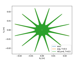
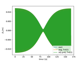
Figure 4.1: Left: horizontal projection of $X_{0},Y_{0}$ components of pendulum movement for $1000\,$s for the exact (exct), averaged (avg) and higher order (HO) averaged models. Right: Vertical projection of $Z_{0}$ component of pendulum movement over time $t$ for $167\,$s (corresponding approximately to the first of six modulation cycles).

4.1 Large scale dynamics, smoothing behavior and stability

First, we verify that the solutions of our phase averaged models stay close to the corresponding exact solutions and capture the same characteristics typical to the swinging spring model (given, for instance, by the stepwise precision of the pendulum in the $(x,y)$-plane). To this end, we compare for a long term simulation of $1000\,$s the solutions in $\mathbf{U}_{0}$ of the exact model, the averaged one with $p=0$ that corresponds to Peddle et al. (2019) and a higher order (HO) version with, e.g., $p=6$. In order to guarantee stable simulations, we reset the higher order values in $\mathbf{U}_{i}$ (or $\mathbf{V}_{i}$), $i=1,...p$, to zero, here after a resetting time of $\Delta T=100\,$s. The size of this resetting window $\Delta T$ does only marginally impact the accuracy (cf. Figure 4.6) but resetting prevents the averaged solutions to become unstable, in particular for large $p$ and long simulations (cf. Figure 4.2).

Large scale dynamics.

In Figure 4.1 (left) we see the projection of the pendulum movement onto the horizontal $(x,y)$-plane. Both, the solutions for the averaged and HO averaged models are very close to the exact solutions, almost indistinguishable in the given figures that show the large scale dynamics. Here, we used an averaging window of $T=0.5\,$s while for smaller $T$ the accuracy does increase (cf. e.g. Figure 4.5). In particular, the solutions of the averaged models capture very well the stepwise precision of the swinging spring model. In the right panel, the movement of the pendulum in the $Z$ axis versus time is shown. Also here, both averaged and HO averaged solutions are very close to the exact one. The figure illustrates nicely fast oscillations with a slowly varying amplitude envelope. This typical behavior of the swinging spring model makes it thus a perfect test problem for our averaging method developed above.

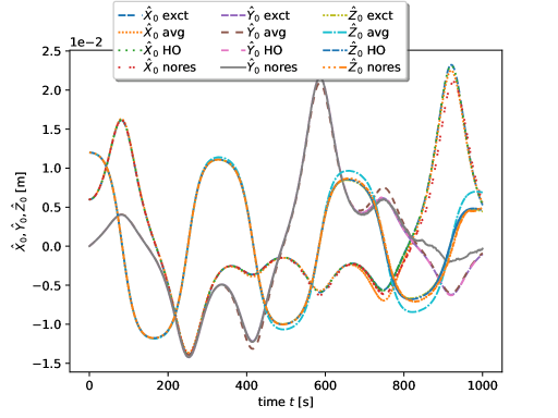
Figure 4.2: $\hat{X}_{0},\hat{Y}_{0},\hat{Z}_{0}$ solutions of the exact (exct), averaged (avg with $p=0$) and higher order (HO) models (with $p=8$) and $T=0.2\,$s; reset every $\Delta T=100\,$s or with no resetting (nores). Here, no resetting leads to instabilities for high $p\geq 8$ after about $800\,$s.

Smoothing properties.

Next, we illustrate how the proposed averaging algorithm filters fast motions from the dynamics of the swinging spring model while still accounting for their effect on the slow dynamics. Given the factorization assumption (2.2) that underlies equations (2.3), it is useful to study in more detail solutions in terms of the velocity $\mathbf{V}$ because the latter provide solutions of the slow dynamics without most of the fast oscillations intrinsic to $\mathbf{U}$. As such, $\mathbf{V}$ (in particular $\mathbf{V}_{0}$) allows us to clearly illustrate how the averaging method filters fast oscillations and how the higher order methods better approximate small scale oscillations around the slow dynamics.

Figure 4.2 shows the solutions for $\hat{X}_{0},\hat{Y}_{0},\hat{Z}_{0}$ of the exact, the averaged, and the HO averaged models without resetting and with resetting at $\Delta T=100\,$s. We use an averaging window of $T=0.2\,$s and $p=8$ for the HO method as this provides sufficiently accurate solutions (cf. Figure 4.5). The figure illustrates also a solutions of the HO model for $p=8$ ($\hat{X}_{0}$ nores, $\hat{Y}_{0}$ nores, $\hat{Z}_{0}$ nores) that becomes slightly unstable after about $800\,$s in case no resetting is used. This instability, however, is easily controlled by simple resetting the higher order velocity component at each $\Delta T$ to zero, resulting in the stable solutions $\hat{X}_{0}$ HO, $\hat{Y}_{0}$ HO, $\hat{Z}_{0}$ HO.

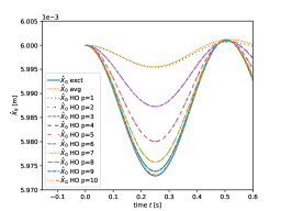
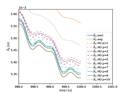
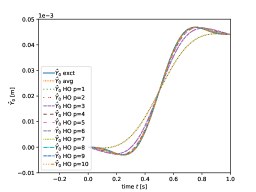
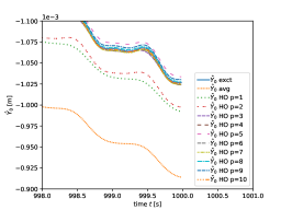
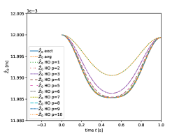
Figure 4.3: $\hat{X}_{0},\hat{Y}_{0},\hat{Z}_{0}$ solutions of the exact (exct), averaged (avg with $p=0$) and higher order (HO) models with resetting ($\Delta T=100\,$s) and averaging window $T=0.15\,$s.

Next, we compare the exact solutions in all three components with those of the averaged models. We realize that for longer simulation times, the averaged solutions slightly drift away from the exact ones, as shown on the right panels in Figure 4.3. This is particularly obvious in the $\hat{Z}_{0}$ component. Further in this figure, we see clearly that with increasing approximation order $p$ the solutions’ drift reduces significantly whilst the small scale oscillations are better approximated. Note that the standard averaging method with $p=0$ corresponds to the original version as introduced in Haut and Wingate (2014). As discussed therein, the averaging leads to some drift away from the exact solutions. As the figure illustrates clearly, including the higher averaging terms significantly reduces this drift while providing solutions much closer to the exact ones.

When considering short integration times, as shown on the left panels in Figure 4.3, it is particularly obvious that the higher order method more accurately approximates small scale oscillations than the standard method. While both approximate well the slower dynamics, the standard averaging method almost entirely smooths out the faster oscillations while with increasing polynomial approximation order, these fast oscillations are better captured by the solutions of the HO averaging models.

4.2 Convergence and accuracy of the higher order models

Here, we study the accuracy of solutions obtained from our higher order averaging method compared to exact solutions, obtained from numerical simulations of (2.3), by performing a convergence analysis of the solutions and their dependencies on the averaging window $T$ and the polynomial degree $p$. For the chosen $T$ from above, we already verified that with increasing $p$ the error in the averaged solutions decreases significantly. However, these error depend crucially on the choice of averaging window $T$. For instance, in case $T$ is too large, even high polynomial approximations will have an significant error.

In the following, we will therefore study solution errors with respect to both $p$ and $T$ and provide a 2 dimensional (2D) error map. To determine these 2D error maps, we define the following $L_{2}$ error measure for solution $\hat{X}(t)$ (and similarly for $\hat{Y}(t),\hat{Z}(t)$)

$${L_{2}}\hat{X}(t)=\frac{\sqrt{\int_{0}^{tf}(\hat{X}(t)-\hat{X}_{e}(t))^{2}dt}}{\sqrt{\int_{0}^{tf}\hat{X}_{e}(t)^{2}dt}}$$ (4.1)

where $\hat{X}(t)$ and $\hat{X}_{e}(t)$ is the x-component of $\mathbf{V}$ of the averaged and exact solutions, respectively (and similarly for $\hat{Y},\hat{Z}$), and where $tf$ is the final time.

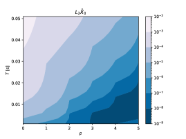
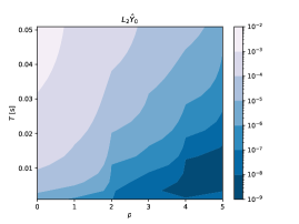
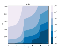
Figure 4.4: 2D $L_{2}$-error plots $(p,T)$ for solutions $\mathbf{V}_{0}$ in the limit $T\rightarrow 0\,$s. Noting the logarithmic colour scale, we note that the error decays exponentially with $p$ for fixed $T$, and larger $T$ reduces the decay rate.

We will consider three regimes of averaging window size $T$, namely (i) $T\rightarrow 0\,$s, (ii) $T\in[0.05,0.5]\,$s, and (iii) $T\rightarrow\infty$, whilst studying the impact of higher order polynomial approximation in the solver on the solutions’ accuracy. In practice, we achieve with our implementation and, e.g., $p=5$ values for $T$ of about $0.0005\,$s for case (i) and of $1e+12\,$s for case (iii), or even smaller respectively larger $T$ for smaller $p$. We will consider an integration time of $tf=167\,$s here (corresponding to the first cycle) and we use the default adaptive timestepping error tolerance of $1.49012e^{-8}$ or otherwise stated.

In Figure 4.4 we presented results for case (i) for small $T\in[0.001,0.0035,0.0060,...,0.05]\,$s. The figure indicates that for $T\approx 0.005\,$s we have minimum error values in $\hat{X}_{0},\hat{Y}_{0},\hat{Z}_{0}$ of about $10^{-9}$ for $p=5$. With these values we reach the default solver tolerance ($\approx 10^{-8}$), while with a solver tolerance of about $10^{-10}$, we reach for the same $p$ and $T$ values minimum errors of about $10^{-11}$ that show a similar error pattern to Figure 4.4. With even smaller tolerances the solutions become even more accurate (not shown). For each tolerance studied, we experience for values of $T$ smaller than about $0.0025\,$s an increase in the error values (cf. smallest $T$ values in Figure 4.4). This increase is related to the fact that for $T\leq 0.0025\,$s the condition number of the inverse of $M$ gets huge, leading to increased numerical errors in the numerical solver of the ODE. These results confirm the discussion of Section 2.2.2.

Next, we investigate case (ii). As shown in Figure 4.5, for averaging window sizes smaller than $T\leq 0.2\,$s, the higher order method significantly improves the accuracy (cf. also Figures 4.2 and 4.3). In particular for $T=0.05\,$s and $p=10$ we reach solver tolerance for all three components, but also for other values with $T\leq 0.2\,$s, our method improves the accuracy significantly. For values $0.2\,$s$\,\leq T\leq 0.5\,$s, the HO method still provides improvements but with error values for $p=10$ of $10^{-02}$ and $10^{-03}$ for $\hat{X}_{0},\hat{Y}_{0}$ and $\hat{Z}_{0}$, respectively. For even larger averaging windows of $T\geq 0.5\,$s (case (iii)), solutions share these latter error values even for larger values in $p$ (not shown). This is because in this case, the exponential function dominates the factors in the expansion in (2.34) and, therefore, the results correspond to the original averaging method of Peddle et al. (2019). Also these results agree with the derivations of Section 2.2.2.

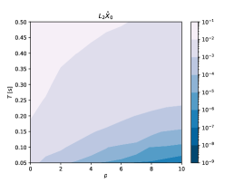
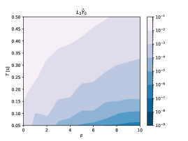
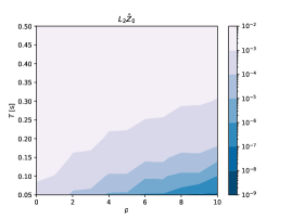
Figure 4.5: 2D $L_{2}$-error plots $(p,T)$ for $\mathbf{V}_{0}$ for intermediate values of $T$.

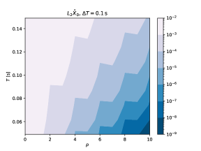
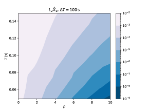
Figure 4.6: 2D $L_{2}$-error plots $(p,T)$ for $\hat{X}_{0}$ for resetting windows $\Delta T=0.1\,s$ (left) and $\Delta T=100\,s$ (right).

As indicated above, the resetting after the time interval $\Delta T$ of the higher order velocity components prevents the HO models from blowups. The latter are due to instabilities in the higher order terms which, in turn, are caused by a growing discrepancy between principal and higher order modes in $\mathbf{V}$ that might happen after long simulation times, cf. Figure 4.2. In Figure 4.6, we present error plots for $\hat{X}_{0}$ solutions obtained with the higher order averaging approach for two different resetting values: $\Delta T=0.1\,$s (left) and $\Delta T=100\,$s (right). The similarity of both error maps indicates that a change in the resetting window size $\Delta T$ has almost no impact on the accuracy of the solutions. This property is shared by the corresponding error maps for the $\hat{Y}_{0}$ and $\hat{Z}_{0}$ components (not shown).

5 Summary and outlook

In this paper we introduced a higher order finite window averaging technique and investigated it by specialising to Gaussian weight functions to allow for explicit computation of averages. This enabled us to efficiently investigate the higher order technique when applied to highly oscillatory ODEs, in particular Lynch’s swinging spring model. We found that higher order corrections can strongly increase the accuracy of the averaged model solutions, but only when the averaging window is close to the time period of the fast frequency (this model only has two fast frequencies, in 2:1 resonance). We expect the situation to become more complicated when there are a spectrum of fast frequencies. In this case, it is known that very high frequencies do not change the slow components of the solution much, but moderate fast frequencies can resonate in the nonlinearity (just like in the swinging spring), altering the slow dynamics. In this case one would want to select an averaging window that removes as much fast dynamics as possible, whilst preserving accuracy of the slow dynamics arising from near-resonant interactions, and the higher order model could prove useful in reducing the impact of the averaging on this slow dynamics.

In this paper we have also avoided numerical aspects, such as the effects of approximate averages by numerical quadrature, and the interaction of numerical time integrators with the averaging. Haut and Wingate (2014) investigated the impact of using numerical quadrature in the basic phase averaging setting (corresponding to the lowest order method in the present framework) and found that there are no numerical instabilities provided that the oscillations in the phase variable are sufficiently resolved by the quadrature (the Nyquist condition, essentially). In the present framework, choosing a different $\rho$, or using numerical quadrature, just results in a different inner product with which to compute the projections, so we do not anticipate difficulties. An analysis using the ideas of Peddle et al. (2019) would be useful to address the interaction of numerical time integrators with the averaging. Looking further ahead, if the higher order averaging model is shown to improve the accuracy of averaging methods whilst still allowing larger time steps in numerical integrations, this would motivate the investigation of multilevel schemes such as PFASST, where the low order averaging is used as a coarse propagator and higher order averaging models provide higher order corrections, some of which can be hidden in parallel behind first iterations in later timesteps.

Appendix A Fully explicit representation for $p=2$

Here, we present a fully explicit version of (2.39) in terms of tendencies for $\mathbf{V}_{0}$, $\mathbf{V}_{1}$, and $\mathbf{V}_{2}$. Split into these tendencies while inserting values for $\mathrm{R}_{\alpha}^{m}$ and taking into account that $\mathbf{F}_{m,j,k}=\mathbf{F}_{m,k,j}\forall m,j,k$, we arrive at

$$\begin{split}\dot{\mathbf{V}}_{0}(t)=&\sum_{m=1}^{M}e^{ic_{m}t}e^{-\frac{c_{m}^{2}T^{2}}{2}}\Big{(}\frac{3}{2}\mathbf{F}_{m,0,0}1+\frac{3}{2}\mathbf{F}_{m,1,1}(T^{2}-k_{m}^{2}T^{4})+\frac{3}{2}\mathbf{F}_{m,2,2}(3T^{4}-6k_{m}^{2}T^{6}+k_{m}^{4}T^{8})\\ &+3\mathbf{F}_{m,0,1}(ic_{m}T^{2})+3\mathbf{F}_{m,0,2}(T^{2}-k_{m}^{2}T^{4})+3\mathbf{F}_{m,1,2}(i3k_{m}T^{4}-ik_{m}^{3}T^{6})\\ &-\frac{1}{2}\mathbf{F}_{m,0,0}(1-k_{m}^{2}T^{2})-\frac{1}{2}\mathbf{F}_{m,1,1}(3T^{2}-6k_{m}^{2}T^{4}+k_{m}^{4}T^{6})\\ &-\frac{1}{2}\mathbf{F}_{m,2,2}(15T^{4}-45k_{m}^{2}T^{6}+15k_{m}^{4}T^{8}-k_{m}^{6}T^{10})-\mathbf{F}_{m,0,1}(i3k_{m}T^{2}-ik_{m}^{3}T^{4})\\ &-\mathbf{F}_{m,0,2}(3T^{2}-6k_{m}^{2}T^{4}+k_{m}^{4}T^{6})-\mathbf{F}_{m,1,2}(i15k_{m}T^{4}-i10k_{m}^{3}T^{6}+ik_{m}^{5}T^{8})\big{)},\end{split}$$

which can be summarized to

$$\begin{split}\dot{\mathbf{V}}_{0}(t)=&\sum_{m=1}^{M}e^{ic_{m}t}e^{-\frac{c_{m}^{2}T^{2}}{2}}\Big{(}\mathbf{F}_{m,0,0}(1+\frac{1}{2}c_{m}^{2}T^{2})+\mathbf{F}_{m,1,1}(\frac{3}{2}c_{m}^{2}T^{4}-\frac{1}{2}c_{m}^{4}T^{6})\\ &+\mathbf{F}_{m,2,2}(-3T^{4}+\frac{27}{2}c_{m}^{2}T^{6}-6c_{m}^{4}T^{8}+\frac{1}{2}c_{m}^{6}T^{8})\\ &+\mathbf{F}_{m,0,1}(ic_{m}^{3}T^{4})+\mathbf{F}_{m,0,2}(3c_{m}^{2}T^{4}-c_{m}^{4}T^{6})+\mathbf{F}_{m,1,2}(-6ic_{m}T^{4}+7ic_{m}^{3}T^{6}-ic_{m}^{5}T^{8})\Big{)}.\end{split}$$

For $\mathbf{V}_{1}$, there follows directly

$$\begin{split}\dot{\mathbf{V}}_{1}(t)=&\sum_{m=1}^{M}e^{ic_{m}t}e^{-\frac{c_{m}^{2}T^{2}}{2}}\Big{(}\mathbf{F}_{m,0,0}(ic_{m})+\mathbf{F}_{m,1,1}(i3c_{m}T^{2}-ic_{m}^{3}T^{4})+\mathbf{F}_{m,2,2}(i15c_{m}T^{4}-i10c_{m}^{3}T^{6}+ic_{m}^{5}T^{8})\\ &+2\mathbf{F}_{m,0,1}(1-c_{m}^{2}T^{2})+2\mathbf{F}_{m,0,2}(i3c_{m}T^{2}-ic_{m}^{3}T^{4})+2\mathbf{F}_{m,1,2}(3T^{2}-6c_{m}^{2}T^{4}+c_{m}^{4}T^{6})\Big{)}.\end{split}$$

Finally for $\mathbf{V}_{2}$, we find

$$\begin{split}\dot{\mathbf{V}}_{2}(t)=&\sum_{m=1}^{M}e^{ic_{m}t}e^{-\frac{c_{m}^{2}T^{2}}{2}}\Big{(}-\frac{1}{2}\mathbf{F}_{m,0,0}1/T^{2}-\frac{1}{2}\mathbf{F}_{m,1,1}(T^{0}-k_{m}^{2}T^{2})-\frac{1}{2}\mathbf{F}_{m,2,2}(3T^{2}-6k_{m}^{2}T^{4}+k_{m}^{4}T^{6})\\ &-\mathbf{F}_{m,0,1}(ik_{m}T^{0})-\mathbf{F}_{m,0,2}(T^{0}-k_{m}^{2}T^{2})-\mathbf{F}_{m,1,2}(i3k_{m}T^{2}-ik_{m}^{3}T^{4})\\ &+\frac{1}{2}\mathbf{F}_{m,0,0}(1/T^{2}-k_{m}^{2}T^{0})+\frac{1}{2}\mathbf{F}_{m,1,1}(3T^{0}-6k_{m}^{2}T^{2}+k_{m}^{4}T^{4})\\ &+\frac{1}{2}\mathbf{F}_{m,2,2}(15T^{2}-45k_{m}^{2}T^{4}+15k_{m}^{4}T^{6}-k_{m}^{6}T^{8})\\ &+\mathbf{F}_{m,0,1}(i3k_{m}T^{0}-ik_{m}^{3}T^{2})+\mathbf{F}_{m,0,2}(3T^{0}-6k_{m}^{2}T^{2}+k_{m}^{4}T^{4})\\ &+\mathbf{F}_{m,1,2}(i15k_{m}T^{2}-i10k_{m}^{3}T^{4}+ik_{m}^{5}T^{6})\Big{)},\end{split}$$

which leads to

$$\begin{split}\dot{\mathbf{V}}_{2}(t)=&\sum_{m=1}^{M}e^{ic_{m}t}e^{-\frac{c_{m}^{2}T^{2}}{2}}\Big{(}\mathbf{F}_{m,0,0}(-\frac{1}{2}c_{m}^{2})+\mathbf{F}_{m,1,1}(1-\frac{5}{2}c_{m}^{2}T^{2}+\frac{1}{2}c_{m}^{4}T^{4})\\ &+\mathbf{F}_{m,2,2}(6T^{2}-\frac{39}{2}c_{m}^{2}T^{4}+7c_{m}^{4}T^{6}-\frac{1}{2}c_{m}^{6}T^{8})\\ &+\mathbf{F}_{m,0,1}(2ic_{m})+\mathbf{F}_{m,0,2}(2-5c_{m}^{2}T^{2}+c_{m}^{4}T^{4})+\mathbf{F}_{m,1,2}(12ic_{m}T^{2}-9ic_{m}^{3}T^{4}+ic_{m}^{5}T^{6})\Big{)}.\end{split}$$

References

- Abdulle et al. (2012) Abdulle, A., Weinan, E., Engquist, B., Vanden-Eijnden, E., 2012. The heterogeneous multiscale method. Acta Numerica 21, 1–87.
- Ariel et al. (2009) Ariel, G., Engquist, B., and Tsai, R. 2009. A multiscale method for highly oscillatory ordinary differential equations with resonance. Mathematics of Computation, 78 (266), 929-956.
- Ariel et al. (2016) Ariel, G., Kim, S. J., and Tsai, R. 2009. Parareal multiscale methods for highly oscillatory dynamical systems. SIAM Journal on Scientific Computing, 38 (6), A3540–A3564.
- Babin et al. (1997) Babin, A., Mahalov, A., Nicolaenko, B., Zhou, Y., Jun 1997. On the asymptotic regimes and the strongly stratified limit of rotating boussinesq equations. Theoretical and Computational Fluid Dynamics 9 (3), 223–251.
- Caliari et al. (2021) Caliari, M., Einkemmer, L., Moriggl, A., Ostermann, A., 2021. An accurate and time-parallel rational exponential integrator for hyperbolic and oscillatory pdes. Journal of Computational Physics 437, 110289.
- Charney et al. (1950) Charney, J. G., Fjortoft, R., von Neumann, J., 1950. Numerical Integration of the Barotropic Vorticity Equation. Tellus 2, 237–254.
- Davies et al. (2003) Davies, T., Staniforth, A., Wood, N., and Thuburn, J., 2003. Validity of anelastic and other equation sets as inferred from normal-mode analysis. Quarterly Journal of the Royal Meteorological Society 129 (593), 2761–2775.
- Enquist and Tsai (2005) Engquist, B., and Tsai, Y.. ”Heterogeneous multiscale methods for stiff ordinary differential equations.” Mathematics of computation 74.252 (2005): 1707-1742.
- Haut and Wingate (2014) Haut, T., Wingate, B., 2014. An asymptotic parallel-in-time method for highly oscillatory PDEs. SIAM Journal on Scientific Computing 36 (2), A693–A713.
- Haut et al. (2016) Haut, T. S., Babb, T., Martinsson, P., Wingate, B., 2016. A high-order time-parallel scheme for solving wave propagation problems via the direct construction of an approximate time-evolution operator. IMA Journal of Numerical Analysis 36 (2), 688–716.
- Holm and Lynch (2002) Holm, D. D., Lynch, P., 2002. Stepwise precession of the resonant swinging spring. SIAM Journal on Applied Dynamical Systems 1 (1), 44–64.
- Jones et al. (1999) Jones, D., Mahalov, a., Nicolaenko, B., 1999. A Numerical Study of an Operator Splitting Method for Rotating Flows with Large Ageostrophic Initial Data. Theoretical and Computational Fluid Dynamics 13 (2), 143.
- Kevrekidis et al. (2003) Kevrekidis, I. G., Gear, C. W., Hyman, J. M., Kevrekidis, P. G. et al, 2003. Equation-free, coarse-grained multiscale computation: Enabling mocroscopic simulators to perform system-level analysis. Communications in Mathematical Sciences, 1 (4), 715–762.
- Majda and Embid (1998) Majda, A. J., Embid, P., 1998. Averaging over fast gravity waves for geophysical flows with unbalanced initial data. Theoretical and computational fluid dynamics 11 (3-4), 155–169.
- Minion (2011) Minion, M., 2011. A hybrid parareal spectral deferred corrections method. Communications in Applied Mathematics and Computational Science 5 (2), 265–301.
- Peddle et al. (2019) Peddle, A. G., Haut, T., Wingate, B., 2019. Parareal convergence for oscillatory PDEs with finite time-scale separation. SIAM Journal on Scientific Computing 41 (6), A3476–A3497.
- Sanders et al. (2007) Sanders, J. A., Verhulst, F., Murdock, J., 2007. Averaging methods in nonlinear dynamical systems, 2nd Edition. Applied mathematical sciences. Springer, New York, Berlin, Heidelberg.
- Schochet (1994) Schochet, S., 1994. Fast singular limits of hyperbolic pdes. Journal of differential equations 114 (2), 476–512.
- Schreiber et al. (2018) Schreiber, M., Peixoto, P. S., Haut, T., Wingate, B., 2018. Beyond spatial scalability limitations with a massively parallel method for linear oscillatory problems. The International Journal of High Performance Computing Applications 32 (6), 913–933.
- Smith and Waleffe (2002) Smith, L. M., Waleffe, F., 2002. Generation of slow large scales in forced rotating stratified turbulence. Journal of Fluid Mechanics 451, 145–168.
- Tao et al. (2010) Tao, M., Owhadi, H., and Marsden, J. E., 2010. Nonintrusive and structure preserving multiscale integration of stiff ODEs, SDEs, and Hamiltonian systems with hidden slow dynamics via flow averaging. Multiscale Modeling and Simulation 8 (4), 1269-1324.
- Wingate et al. (2011) Wingate, B. A., Embid, P., Holmes-Cerfon, M., Taylor, M. A., 2011. Low Rossby limiting dynamics for stably stratified flow with finite froude number. Journal of fluid mechanics 676, 546–571.