Template banks based on $\mathbb{Z}^{n}$ and $A_{n}^{*}$ lattices

Abstract

Matched filtering is a traditional method used to search a data stream for signals. If the source (and hence its $n$ parameters) are unknown, many filters must be employed. These form a grid in the $n$-dimensional parameter space, known as a template bank. It is often convenient to construct these grids as a lattice. Here, we examine some of the properties of these template banks for $\mathbb{Z}^{n}$ and $A_{n}^{*}$ lattices. In particular, we focus on the distribution of the mismatch function, both in the traditional quadratic approximation and in the recently-proposed spherical approximation. The fraction of signals which are lost is determined by the even moments of this distribution, which we calculate. Many of these quantities we examine have a simple and well-defined $n\to\infty$ limit, which often gives an accurate estimate even for small $n$. Our main conclusions are the following: (i) a fairly effective template-based search can be constructed at mismatch values that are shockingly high in the quadratic approximation; (ii) the minor advantage offered by an $A_{n}^{*}$ template bank (compared to $\mathbb{Z}^{n}$) at small template separation becomes even less significant at large mismatch. So there is little motivation for using template banks based on the $A_{n}^{*}$ lattice.

I Introduction

Matched filtering is a standard technique WZ ; Hels used to search for weak gravitational-wave signals from the binary inspiral of black holes and/or neutron stars. This compares the data (suitably weighted in frequency space) to a template of the expected waveform Schutz:1989yw ; Sathyaprakash:1991mt ; Schutz_Book ; Cutler:1992tc ; Sathyaprakash:1994nj ; Cutler:1994ys ; Dhurandhar:1992mw ; Dhurandhar:1994mi ; Balasubramanian:1994uy ; Balasubramanian:1995bm ; Owen:1998dk ; FINDCHIRP . Matched filtering is also used to search for weak electromagnetic (radio and gamma-ray) Nieder and gravitational-wave signals from rapidly rotating neutron stars (pulsars) cartel and has many other applications across a broad range of fields and topics.

Because these searches are typically looking for new events and/or unknown sources, the parameters of the signals are not known. Some examples of these parameters include sky position, mass, and spin or chirp frequency. Thus, a collection of templates must be employed. The grid of these templates in parameter space is generally referred to as a “template bank”.

If the parameter space is low-dimensional and the parameter-space volume is not too large, one can simply “overcover” the space, putting many redundant templates close together. However, if the parameter-space dimension and/or volume is large, this quickly becomes (computationally speaking) very expensive. On the other hand, if the templates are spaced too far apart, then it’s possible that some signals be missed, because there was no template in the bank which matched the waveform well enough. Thus, a compromise must be reached: enough templates must be employed that signals are not lost, but the number of templates must not be so large that the computing cost explodes. For some searches (e.g., for continuous gravitational waves from neutron stars in binary systems) the computing cost is so high that it constrains the search sensitivity.

The problem of how to place templates in parameter space is well studied. There are many ways to construct template banks. For example, one can simply place the templates at random MessengerPrixPapa , with a high enough density that most signals are likely to lie near enough to a template. Or one can improve this by removing redundant templates which are “too close” to neighboring ones, and adding more templates at random, if required AllenHarrySathya . Alternatively, one can build a template bank as a regular lattice in parameter space. Two examples of such lattices are the $\mathbb{Z}^{n}$ and $A_{n}^{*}$ lattices. The first of these is just the Cartesian product of equally spaced grids in all dimensions, and the second is the $n$-dimensional generalization of the two-dimensional hexagonal lattice and the three-dimensional face-centered cubic (fcc) lattice.

One way to characterize a template bank is via the mismatch function $m$. This is a function on parameter space, which quantifies how much signal-to-noise ratio (SNR) is lost because of the discreteness of the template bank. Its value at any point is the fractional difference between the squared SNR obtained for a signal with those parameters, and the squared SNR that would have been obtained had a template been located at that point. Thus, $m$ vanishes at the locations of the templates, and is largest “halfway in-between” two templates. In a recent paper, we show how the fraction of lost signals is related to the average of $m$ and functions of $m$ NewAllenPaper .

When the templates are close together, and the mismatch is small, $m$ can be expressed as a positive-definite quadratic form and thought of as the squared distance between the parameter-space point and the closest template. Thus, in this approximation, $m\approx g_{ab}\Delta\lambda^{a}\Delta\lambda^{b}$, where $g_{ab}$ is the metric on the parameter space and $\Delta\lambda^{a}$ is the coordinate separation between the two points (see, e.g., Owen ; Owen:1998dk ). Here, we call this the quadratic approximation to the mismatch, and write it as $m=r^{2}$. When the templates are less-closely spaced, a better approximation to the mismatch is the “spherical” ansatz, $m\approx\sin^{2}r=\sin^{2}(\sqrt{g_{ab}\Delta\lambda^{a}\Delta\lambda^{b}})$, recently introduced in AllenSpherical .

If the mismatch is small, then the bank which minimizes the average second-moment of $r^{2}$ loses the smallest fraction of signals NewAllenPaper . If the bank is a lattice, this is called the “optimal quantizer” Conway . This paper extends those results to large mismatch, by exploiting the spherical ansatz AllenSpherical , and carrying out an explicit calculation for template banks constructed from the $\mathbb{Z}^{n}$ and $A_{n}^{*}$ lattices.

Our paper is organized as follows. In Sec. II we describe the $n$-dimensional lattices $\mathbb{Z}^{n}$ and $A_{n}^{*}$, and derive their key properties. In Sec. III we calculate the fraction of lost detections in the quadratic and spherical approximations for these lattices for $2$- and $3$-dimensional source distribution. This fraction of lost signals may be thought of as the “inefficiency” or “loss fraction” of the lattice. In Sec. IV we evaluate the loss fraction as the parameter space dimension $n\to\infty$. This gives simple analytic expressions; in some cases the approach is fast enough that these are good approximations even in finite numbers of dimensions. In Sec. V we compare the loss fraction of $\mathbb{Z}^{n}$ and $A_{n}^{*}$ at fixed computing cost. Finally, in Sec. VI, we examine the distribution function of the squared radius $r^{2}$, and its properties for the $\mathbb{Z}^{n}$ and $A_{n}^{*}$ lattices. This is followed by a short Conclusion.

Our results only depend on the even-order moments of the Wigner-Seitz (WS) cells of the lattices, which we denote by $\langle r^{2m}\rangle$. Appendix A contains a calculation of these moments for the $\mathbb{Z}^{n}$ lattice, and Appendix B contains the corresponding calculation for the $A_{n}^{*}$ lattice.

II The $\mathbb{Z}^{n}$ and $A_{n}^{*}$ lattices

The lattices $\mathbb{Z}^{n}$ and the $A_{n}^{*}$ are an infinite collection of regularly-spaced points in Cartesian space $\mathbb{R}^{n}$. We use $x$ to denote a point in $\mathbb{R}^{n}$ with the normal Euclidean norm ${|{\mbox{\boldmath$x$}}|}^{2}={\mbox{\boldmath$x$}}\cdot{\mbox{\boldmath$x$}}$, where the dot denotes the standard dot product. The lattices are generated by a set of $n$ basis vectors ${\mbox{\boldmath$e$}}_{i}\in\mathbb{R}^{n}$, for $i\in 1,\cdots,n$, which for these particular lattices are normalized so that ${\mbox{\boldmath$e$}}_{i}\cdot{\mbox{\boldmath$e$}}_{i}=1$. Two-dimensional representatives of these lattices are illustrated in Fig. 1.

$$\hskip 49.79231pt({\bf a})\hskip 187.78836pt({\bf b})$$

Figure 1: Two-dimensional lattices $(\ell=1)$: (a) the $\mathbb{Z}^{2}$ square lattice, (b) the $A_{2}^{*}$ hexagonal lattice. The fundamental polytropes are shown in light grey, the WS cells are shown in dark grey and inscribed by the dashed circles of the covering radius. For general $n$, the basis vectors ${\mbox{\boldmath$e$}}_{i}$ for $A_{n}^{*}$ define vertices of an equilateral $n$-simplex (see text after Eq. (10)).

To characterize the geometry of the lattice, we shall use $x_{i}$ to denote Cartesian coordinates and $y_{i}$ to denote lattice coordinates. Accordingly, the lattice consists of all points ${\mbox{\boldmath$x$}}=y_{i}{\mbox{\boldmath$e$}}_{i}$ in $\mathbb{R}^{n}$, such that $y_{i}=c_{i}\ell$, where $c_{i}\in\mathbb{Z}$ are integers and $\ell$ is the lattice spacing. These points are called lattice vertices. From here forward, we shall use the “summation convention” that repeated indices are summed.

The squared distance $r^{2}$ between points ${\mbox{\boldmath$x$}}_{A}$ and ${\mbox{\boldmath$x$}}_{B}$ with lattice coordinates $y_{Ai}$ and $y_{Bi}$ is then

$$r^{2}=({\mbox{\boldmath$x$}}_{A}-{\mbox{\boldmath$x$}}_{B})\cdot({\mbox{\boldmath$x$}}_{A}-{\mbox{\boldmath$x$}}_{B})=\Delta y_{i}\Delta y_{j}{\mbox{\boldmath$e$}}_{i}\cdot{\mbox{\boldmath$e$}}_{j}=g_{ij}\Delta y_{i}\Delta y_{j}\,,$$ (1)

where $\Delta y_{i}=y_{Ai}-y_{Bi}$ are the lattice coordinate separations and the (flat) metric is $g_{ij}={\mbox{\boldmath$e$}}_{i}\cdot{\mbox{\boldmath$e$}}_{j}$.

The region of $\mathbb{R}^{n}$ for which the coordinates $y_{i}$’s are such that $|y_{i}|\in[0,\ell]$, is called a “Fundamental Polytope” or FP. The FP has $2^{n}$ vertices, which are neighboring lattice points. The region of $\mathbb{R}^{n}$ which is closer [in the sense of the coordinate distance Eq. (1)] to a given lattice point than to any other lattice point is called the “Wigner-Seitz cell” (WS) of that lattice point. We also denote the Wigner-Seitz cell of the origin $y_{i}=0$ by WS (see Fig. 1). The distance from the origin to the most distant point of the WS is called the covering radius or WS radius $R$; it is the radius of the smallest sphere about the origin which encloses every point of the WS.

We can compute the $n$-volume of the FP and the WS as follows. Since all FP are equivalent, we concentrate on the fundamental FP defined by lattice coordinate values $y_{i}\in[0,\ell]$. The volume of the FP is

$$V_{\mbox{\tiny FP}}=\int_{0}^{\ell}dy_{1}\cdots\int_{0}^{\ell}dy_{n}\sqrt{g}\,,$$ (2)

where $g=\det(g_{ij})$. The $n$-volume of the WS, $V_{\mbox{\tiny WS}}$, is equal to that of the FP, because (if the WS is copied around all lattice points) they overlap only on the boundaries (a set of measure zero), are in one-to-one correspondence, and cover all of space.

The fundamental FP is contractible to the origin, in the sense that if a point ${\mbox{\boldmath$x$}}\in\mathbb{R}^{n}$ lies inside it, then so does the point $\lambda{\mbox{\boldmath$x$}}$ for $\lambda\in[0,1)$. Because it is defined via a linear construction, it can also be contracted to any other vertex, so it is convex and contractible in any direction. By construction the FP is bounded by a set of $(n-1)$-dimensional planes.

In similar fashion, the boundary of the WS is defined by a set of $(n-1)$-dimensional planes that lie halfway between the origin and the surrounding lattice points. We can compute the covering radius $R$ of the WS centered at the origin by considering the subset of those planes which lie in the FP, i.e. which lie halfway between the origin and the remaining $2^{n}-1$ FP lattice points, and finding the point of intersection most distant from the origin.

To characterize the efficiency of the space covering, one defines the thickness $\Theta$ as the average number of covering spheres that contain a point of the space. This is equal to the ratio of volume of an $n$-dimensional ball enclosed by one of the spheres, to the volume $V_{\mbox{\tiny FP}}=V_{\mbox{\tiny WS}}$ Conway ,

$$\Theta=\frac{V(B_{n}(R))}{V_{\mbox{\tiny WS}}}.$$ (3)

Here, $V(B_{n}(R))=\pi^{n/2}R^{n}/\Gamma(1+n/2)$ is the volume of an $n$-ball $B_{n}$ of radius $R$. From the definition it follows that $\Theta\geq 1$. Smaller values of $\Theta$ indicate less overlap among the balls, i.e. a more efficient covering.

In the following subsections we compute the quantities defined above for the $\mathbb{Z}^{n}$ and $A_{n}^{*}$ lattices. We will use these quantities in calculating the statistical properties of functions of the distance, such as the mismatch, for both the lattices and to compare the derived results.

II.1 The $\mathbb{Z}^{n}$ lattice

The $\mathbb{Z}^{n}$ lattice (see, e.g., Conway ) is generated by orthonormal basis vectors

$${\mbox{\boldmath$e$}}_{i}\cdot{\mbox{\boldmath$e$}}_{j}=\delta_{ij}\,,$$ (4)

where $\delta_{ij}$ is the Kronecker delta, i.e., the metric $g_{ij}$ is the identity matrix. Thus, if the basis vectors are taken as the standard coordinate basis, then the lattice coordinates $y_{i}$ are just the normal Cartesian coordinates and $x_{i}=y_{i}$. The distance function Eq. (1) is

$$r^{2}=\sum_{i=1}^{n}\Delta y_{i}^{2}\,,$$ (5)

and, according to Eq. (2), the $n$-volume of the FP is

$$V_{\mbox{\tiny FP}}=\ell^{n}\,.$$ (6)

According to Eq. (1), the largest distance between any pair of vertices in the FP is $r^{2}=n\ell^{2}$. It is also the largest distance from the origin to a point within the FP.

To find the boundary of the WS centered at the origin, we begin by finding the equations of the planes that lie halfway between the origin and the nearest lattice points at distance $\ell$ from the origin. (The other potential bounding planes are irrelevant because they lie outside.) There are $2n$ of these nearest lattice points. They have coordinates $(0,\cdots,0,\pm\ell,0,\cdots,0)$, where $\ell$ is located in the $j$th position and the remaining $n-1$ coordinates vanish. Using the distance function Eq. (5) we find that the coordinates in the $(n-1)$-dimensional boundary planes satisfy the equation

$$\sum_{i=1}^{n}y_{i}^{2}=(y_{j}\mp\ell)^{2}+\sum_{\begin{subarray}{c}i=1\\ (i\neq j)\end{subarray}}^{n}y_{i}^{2}=\ell^{2}\mp 2\ell y_{j}+\sum_{i=1}^{n}y_{i}^{2}\,.$$

Thus the planes bounding the WS satisfy

$$y_{j}=\pm\ell/2\,.$$ (7)

There are $2n$ such planes, since $j=1,\cdots,n$. These define an $n$-cube which is identical to the FP but shifted by $-\ell/2$ along each coordinate axis, so that its center is at the origin. Note that the result Eq. (7) follows directly from the lattice geometry.

The WS radius $R$ is easily computed. The point of mutual intersection of the $n$ planes with $y_{j}>0$ defines a vertex of the WS. All of the $2^{n}$ vertices of the WS (defined by intersecting each of the possible planes, one for each coordinate, $n$ in total) are at the same distance $R$ from the origin. Hence, the WS covering radius $R$ is the distance of that WS vertex from the origin. Using the expression Eq. (5) gives

$$R^{2}=\frac{1}{4}n\ell^{2}\,$$ (8)

for the covering radius of the $\mathbb{Z}^{n}$ lattice. The $n$-volume of the FP and of the WS can be expressed in terms of $R$, as

$$V_{\mbox{\tiny FP}}=V^{\mathbb{Z}^{n}}_{\mbox{\tiny WS}}=2^{n}n^{-n/2}R^{n}.$$ (9)

Later, we will compare the properties of different lattices at fixed $V_{WS}$.

II.2 The $A_{n}^{*}$ lattice

The $A_{n}^{*}$ lattice is a classical root lattice, whose attractions have been discussed in detail by Prix_2007 . For $n\leq 17$ it is either the thinnest classical root lattice, or close to the thinnest one. (Note however that thinner non-classical lattices have been constructed numerically, by semidefinite optimization in the space of lattices. The current record-holders are listed in Table 2 of Sikiric_2008 .)

The $A_{n}^{*}$ lattice is generated by basis vectors chosen to satisfy (see, e.g., Conway ; RB )

$${\mbox{\boldmath$e$}}_{i}\cdot{\mbox{\boldmath$e$}}_{j}=\begin{cases}1&\text{for }i=j\\ -1/n&\text{for }i\neq j.\end{cases}$$ (10)

The vectors ${\mbox{\boldmath$e$}}_{i}$ are easily visualized: they point from the origin to $n$ of the $n+1$ vertices of an equilateral $n$-simplex. (The unit vector from the origin to the final vertex of the simplex is $-{\mbox{\boldmath$e$}}_{1}-\cdots-{\mbox{\boldmath$e$}}_{n}$, which implies that the center of the simplex lies at the origin of coordinates.)

For this lattice, the distance function Eq. (1) is

$$r^{2} = \sum_{i=1}^{n}\Delta y_{i}^{2}-\frac{1}{n}\sum_{\begin{subarray}{c}i,j=1\\ (i\neq j)\end{subarray}}^{n}\Delta y_{i}\Delta y_{j}\,,$$ (11)

$$= \biggl{(}1+\frac{1}{n}\biggr{)}\sum_{i=1}^{n}\Delta y_{i}^{2}-\frac{1}{n}\biggl{(}\sum_{i=1}^{n}\Delta y_{i}\biggr{)}^{2}\,,$$

and the metric is

$$g_{ij}=\begin{pmatrix}1&-1/n&\cdots&-1/n\\ -1/n&1&\cdots&-1/n\\ \vdots&\vdots&\ddots&\vdots\\ -1/n&-1/n&\cdots&1\end{pmatrix}.$$ (12)

Using recursion and row reduction, or applying Sylvester’s theorem, it is easy to see that the determinant is

$$g=n^{-n}(n+1)^{n-1}\,.$$ (13)

From Eq. (2), one obtains

$$V_{\mbox{\tiny FP}}=n^{-n/2}(n+1)^{(n-1)/2}\ell^{n}$$ (14)

for the $n$-volume of the FP.

We now compute the covering radius $R$, which is the distance from the origin to the most distant point of the WS centered at the origin. To find the boundary of the WS centered at the origin, we first find the equation of the plane that lies halfway between the origin and a lattice point with coordinates $(0,\cdots,0,\ell,\cdots,\ell)$, where the number of zeros is $k$ and the number of $\ell$’s is $n-k$. We take this form for an FP vertex because it is sufficiently general, i.e. according to the distance function form Eq. (11), the coordinates can be permuted without changing the distance value. In contrast to the $\mathbb{Z}^{n}$ lattice, every FP vertex defines a WS boundary planes. After multiplying the squared distance by an overall factor of $n/(n+1)$, the coordinates in the planes satisfy the equation

$$\sum_{i=1}^{n}y_{i}^{2} - \frac{1}{n+1}\biggl{(}\sum_{i}y_{i}\biggr{)}^{2}=\sum_{i=1}^{k}y_{i}^{2}+\sum_{i=k+1}^{n}(y_{i}-\ell)^{2}$$ (15)

$$- \frac{1}{n+1}\biggl{(}\sum_{i=1}^{k}y_{i}+\sum_{i=k+1}^{n}(y_{i}-\ell)\biggr{)}^{2}\,.$$

This expression can be simplified, rearranged, and divided by $2\ell(n-k)/(n+1)$ to obtain

$$\sum_{i=1}^{n}y_{i}=\frac{n+1}{n-k}\sum_{i=k+1}^{n}y_{i}-\frac{k+1}{2}\ell\,.$$

Writing the (unity) coefficient of the l.h.s. as $(n+1)/(n-k)-(k+1)/(n-k)$, and canceling the common terms in the sums, gives

$$\frac{n+1}{n-k}\sum_{i=1}^{k}y_{i}-\frac{k+1}{n-k}\sum_{i=1}^{n}y_{i}=-\frac{k+1}{2}\ell\,.$$

Multiplying this expression by $(n-k)/(k+1)$ yields the following formula, which defines the planes bounding the WS cell:

$$\sum_{i=1}^{n}y_{i}=\frac{n+1}{k+1}\sum_{i=1}^{k}y_{i}+\frac{n-k}{2}\ell\,.$$ (16)

Although we obtained this equation for a specific subset of vertices, it is trivial to obtain the corresponding equation for any vertex, by replacing the sum from $1$ to $k$ with a sum over any $k$ of the coordinates. Changing the sign of $\ell$ gives the corresponding parallel plane bounding the WS on the other side of the origin. For this reason, the WS is sometimes called a “permutohedron” Conway and denoted $P_{n}$.

To obtain the covering radius $R$, we intersect a set of $n$ bounding planes defined by Eq. (16), to identify a point at this radius in the WS. The $k=0$ equation implies

$$\sum_{i=1}^{n}y_{i}=\frac{n\ell}{2}\,.$$ (17)

The $k=1$ equation then implies $y_{1}=\ell/(n+1)$. Combining these with the $k=2$ equation implies $y_{2}=2\ell/(n+1)$. Continuing in this fashion, intersecting all of the planes implies $y_{i}=i\ell/(n+1)$. The squared covering radius of the WS is thus given by

$$R^{2} = \left(1+\frac{1}{n}\right)\sum_{i=1}^{n}y_{i}^{2}-\frac{1}{n}\biggl{(}\sum_{i=1}^{n}y_{i}\biggr{)}^{2}$$ (18)

$$= \left(1+\frac{1}{n}\right)\frac{\ell^{2}}{(n+1)^{2}}(1^{2}+\cdots+n^{2})-\frac{1}{n}\left(\frac{n\ell}{2}\right)^{2}$$

$$= \frac{\ell^{2}}{n(n+1)}\frac{n(n+1)(2n+1)}{6}-\frac{n\ell^{2}}{4}$$

$$= \frac{1}{12}(n+2)\ell^{2}\,.$$

As before, we can express the WS $n$-volume in terms of $R$:

$$V^{A_{n}^{*}}_{\mbox{\tiny WS}}=\left[\frac{12(n+1)}{n(n+2)}\right]^{n/2}(n+1)^{-1/2}R^{n}.$$ (19)

This will be useful later, when we compare lattices at fixed WS volume.

III The fraction of lost detections

A template bank is discrete, so most points in parameter space do not have an exactly matching template. As a result, there is the detection mismatch, which, on average, results in lost detections. Here, $N_{D}$ denotes the total number of sources detectable above a certain SNR threshold, and $N_{\mbox{\tiny lost}}$ is the number of lost detections, in comparison with a closely spaced (ideal) bank that catches all signals.

The fraction of lost detections depends upon the effective dimensionality $d$ of the source distribution. If sources are uniformly placed in a 3-dimensional Euclidean space, then the number of sources $N$ grows as the distance $L$ as $dN\propto L^{2}dL$. Similarly, if they are arranged in a 2-dimensional plane (for example, a thin Galactic disk) then $dN\propto LdL$. So here we define $d$ by $dN\propto L^{d-1}dL$ and assume that the squared SNR is proportional to $1/L^{2}$.

If the volume of parameter space is much larger than a WS cell and the template bank is a lattice, then the fraction of lost detections in the spherical approximation AllenSpherical is given by NewAllenPaper

$$\frac{N_{\mbox{\tiny lost}}}{N_{D}}\approx\frac{1}{V_{\mbox{\tiny WS}}}\int_{\mbox{\tiny WS}}f(r)\,dV,$$ (20)

where the integral is over a single WS cell, and the integrand is

$$f(r)=\begin{cases}1-\cos^{d}r&\text{for }r\leq\pi/2\\ 1&\text{for }r>\pi/2\end{cases}.$$ (21)

The ratio $N_{\mbox{\tiny lost}}/N_{D}$ defines the “loss fraction” of the lattice, i.e. the fraction of potentially-detectable signals which the lattice fails to catch. Equivalently, $1-N_{\mbox{\tiny lost}}/N_{D}$ is the efficiency of the lattice: the expected fraction of potentially detectable signals which are indeed found.

Provided that the WS cell is not too large, so that $R<\pi/2$, the integrand can be expanded in a series, giving a loss fraction

$$\frac{N_{\mbox{\tiny lost}}}{N_{D}} \approx \frac{1}{V_{\mbox{\tiny WS}}}\int_{\mbox{\tiny WS}}\left(1-\cos^{d}(r)\right)\,dV$$ (22)

$$= \frac{d}{2}\langle r^{2}\rangle-\frac{d(3d-2)}{24}\langle r^{4}\rangle+\frac{d(15d^{2}-30d+16)}{720}\langle r^{6}\rangle$$

$$- \frac{d(105d^{3}-420d^{2}+588d-272)}{40320}\langle r^{8}\rangle+\cdots\,.$$

Here,

$$\langle r^{p}\rangle=\frac{1}{V_{\mbox{\tiny WS}}}\int_{\mbox{\tiny WS}}r^{p}\,dV$$ (23)

denotes the normalized $p$’th moment of the lattice.

Provided that the effective dimensionality of the source distribution $d>8/\pi^{2}\approx 0.81$, the quadratic approximation always implies a larger fraction of signals lost than the spherical approximation, because $1-\cos^{d}(r)<r^{2}\,d/2$ on the interval $r\in[0,\pi/2]$.

Appendix A shows how the even moments may be computed for the $\mathbb{Z}^{n}$ lattice. The first six of these, which suffice for this paper, are

$$\langle r^{2}\rangle = \frac{n\ell^{2}}{12}\,,$$

$$\langle r^{4}\rangle = \frac{n\ell^{4}}{720}(5n+4)\,,$$

$$\langle r^{6}\rangle = \frac{n\ell^{6}}{60480}(35n^{2}+84n+16)\,,$$ (24)

$$\langle r^{8}\rangle = \frac{n\ell^{8}}{3628800}(175n^{3}+840n^{2}+656n-96)\,,$$

$$\langle r^{10}\rangle = \frac{n\ell^{10}}{95800320}(385n^{4}+3080n^{3}+5456n^{2}$$

$$+ 352n-768)\,,$$

$$\langle r^{12}\rangle = \frac{n\ell^{12}}{523069747200}(175175n^{5}+2102100n^{4}$$

$$+ 6646640n^{3}+3747744n^{2}-2883712n+35328)\,.$$

We note that all of these quantities can be re-expressed in terms of the covering radius $R^{2}=n\ell^{2}/4$. The corresponding even moments for the $A_{n}^{*}$ lattice are computed in Appendix B, but not repeated here.

In the following we shall consider $d=2$ and $d=3$ dimensional source distributions.

III.1 The $\mathbb{Z}^{n}$ lattice: $d=2$ case

Table 1: The maximal fraction of lost detections $N_{\mbox{\tiny lost}}/N_{D}$ for the $\mathbb{Z}^{n}$ and $A_{n}^{*}$ lattices in small dimensions $n$, for $d=2$ and $d=3$ dimensional source distributions. Note that all lattices have “maximal” WS radius $R=\pi/2$, which means that at a fixed dimension $n$, the WS cells have smaller volume for $\mathbb{Z}^{n}$ than for $A_{n}^{*}$.

	$\mathbb{Z}^{n}$	$\mathbb{Z}^{n}$	$A_{n}^{*}$	$A_{n}^{*}$
n	$d=2$	$d=3$	$d=2$	$d=3$
2	0.558	0.665	0.642	0.736
3	0.579	0.697	0.720	0.816
4	0.589	0.714	0.771	0.863
5	0.595	0.724	0.806	0.893
6	0.599	0.731	0.832	0.914
7	0.602	0.736	0.851	0.928
8	0.605	0.740	0.867	0.939
9	0.606	0.743	0.880	0.948
10	0.608	0.745	0.890	0.954
11	0.609	0.747	0.899	0.960
12	0.610	0.749	0.906	0.964
$n\to\infty$	0.620	0.766	1	1

$$\hskip 85.35826pt({\bf a})\hskip 241.84842pt({\bf b})$$

Figure 2: The fraction of lost detections for the $\mathbb{Z}^{n}$ lattice in dimensions $n=2$ (lower solid curve) and $n=4$ (upper solid curve). For larger $n$ the corresponding curves group very close together; the red dashed curve shows the $n\to\infty$ limit of Eq. (29). The left-hand plot shows a $d=2$ dimensional source distribution and the right-hand plot shows a $d=3$ dimensional distribution. The fraction of lost detections depends upon the spacing of the template bank, which is set by the covering radius $R$; in the spherical approximation AllenSpherical , the worst mismatch $m_{\mbox{\tiny worst}}=\sin^{2}R$. For closely spaced templates (small $R$) no detections are lost. For comparison the quadratic approximation Eq. (26) is shown as a dotted curve. It predicts more lost signals than the spherical approximation suggests. The fraction of lost detections at maximum mismatch $R=\pi/2$ is given in Table 1. As $n\to\infty$ and at covering radius $R=\pi/2$, about 62% of detections are lost for a $d=2$ dimensional source distribution, and about 77% are lost for a $d=3$ dimensional source distribution.

$$\hskip 85.35826pt({\bf a})\hskip 241.84842pt({\bf b})$$

Figure 3: The fraction of lost detections for the $A_{n}^{*}$ lattice in different numbers of dimensions (moving upwards) $n=2,4,10,20,100,1000$. The left-hand plot shows a $d=2$ dimensional source distribution and the right-hand plots shows a $d=3$ dimensional distribution. As in the previous figure, the $n\to\infty$ limit is shown in red, and the plot is restricted to $R\leq\pi/2$. The quadratic approximation is shown as a dotted curve in the limit $n\to\infty$ [see Eq. (33)]. The fraction of lost detections at maximum mismatch $R=\pi/2$ is given in Table 1.

For a source distribution with effective dimensionality $d=2$, we now evaluate the fraction of lost sources, assuming that the covering radius $R\leq\pi/2$. The integrand of Eq. (22) ($f(r)=\sin^{2}r$, the mismatch in the spherical approximation AllenSpherical ) is approximated (within 1% ) by taking terms up to the eighth moment. Then, Eq. (22) takes the form

$$\frac{N_{\mbox{\tiny lost}}}{N_{D}} \approx \langle r^{2}\rangle-\frac{1}{3}\langle r^{4}\rangle+\frac{2}{45}\langle r^{6}\rangle-\frac{1}{315}\langle r^{8}\rangle$$ (25)

$$= \frac{1}{3}R^{2}-\frac{5n+4}{135n}R^{4}+\frac{70n^{2}+168n+32}{42525n^{2}}R^{6}$$

$$-\frac{175n^{3}+840n^{2}+656n-96}{4465125n^{3}}R^{8}.$$

We plot this quantity in Fig. 2(a), where $m_{\mbox{\tiny worst}}=\sin^{2}R$ denotes the worst-case mismatch in the spherical approximation.

Fig. 2(a) also compares the spherical approximation AllenSpherical to the mismatch with the prediction one would find using the normal quadratic approximation. If the lattice is widely spaced (sparse), then the spherical approximation predicts significantly fewer lost signals than the standard quadratic approximation. The quadratic approximation keeps only the first term in Eq. (25), so

$$\left[\frac{N_{\mbox{\tiny lost}}}{N_{D}}\right]_{\text{Quadratic-Approximation}}=\frac{1}{3}\arcsin^{2}(\sqrt{m_{\mbox{\tiny worst}}})\,,$$ (26)

which is valid in any dimension $n$. To enable a fair comparison with the spherical approximation, we need to examine the two expressions for the same lattice, meaning at the same WS radius $R$. So in Eq. (26), this is still related to the worst-case mismatch via the spherical approximation AllenSpherical $m_{\mbox{\tiny worst}}=\sin^{2}R$ (rather than with the quadratic approximation $m_{\mbox{\tiny worst}}=R^{2}$).

Results of numerical computations of the maximal fraction of lost detections are presented in Table 1.

III.2 The $\mathbb{Z}^{n}$ lattice: $d=3$ case

For $d=3$ the integrand in Eq. (22) is $f(r)=1-\cos^{3}r$, and we again assume $R\leq\pi/2$. The expression Eq. (22) takes the following form:

$$\frac{N_{\mbox{\tiny lost}}}{N_{D}} \approx \frac{3}{2}\langle r^{2}\rangle-\frac{7}{8}\langle r^{4}\rangle+\frac{61}{240}\langle r^{6}\rangle-\frac{547}{13440}\langle r^{8}\rangle$$ (27)

$$+ \frac{703}{172800}\langle r^{10}\rangle-\frac{44287}{159667200}\langle r^{12}\rangle\,.$$

Here, to maintain 1% accuracy in the integrand we have had to include more terms than for $d=2$. Fig. 2(b) illustrates how the fraction of lost detections depends on the covering radius (via the worst-case mismatch $m_{\mbox{\tiny worst}}$). In the case of quadratic approximation we keep only the first term in Eq. (27),

$$\left[\frac{N_{\mbox{\tiny lost}}}{N_{D}}\right]_{\text{Quadratic-Approximation}}=\frac{1}{2}\arcsin^{2}(\sqrt{m_{\mbox{\tiny worst}}})\,,$$ (28)

valid in any dimension $n$. For a widely spaced lattice the spherical approximation predicts significantly fewer lost signals than the standard quadratic approximation. The worst-case values (fraction of lost detections at WS radius $R=\pi/2$) are shown in Table 1.

III.3 The $A_{n}^{*}$ lattice: $d=2$ and $d=3$ cases

As for the $\mathbb{Z}^{n}$ lattice, we can again estimate how the fraction of lost detections depends upon the covering radius. For the $A_{n}^{*}$ lattice, we can compute the moments $\langle r^{p}\rangle$ exactly, but cannot give a closed analytic form as we did for the $\mathbb{Z}^{n}$ lattice. We use the exact expressions obtained in Appendix B, and substitute these into the expressions Eq. (25) and Eq. (27). The plots of the fraction of lost detections versus $m_{\mbox{\tiny worst}}$ are given in Fig. 3, and some worst-case values are shown in Table 1.

IV Large $n$ limits

The reader will notice that as the dimension $n$ of the parameter space gets large, the curves appear to approach a limit. This is explained in Sec. VI, where we show that as $n$ gets large, the mismatch distribution function becomes sharply peaked at $r^{2}=R^{2}/3$ for the $\mathbb{Z}^{n}$ lattice and at $r^{2}=R^{2}$ for the $A_{n}^{*}$ lattice. Thus, for the $\mathbb{Z}^{n}$ lattice, Eq. (22) immediately gives

$$\lim_{n\to\infty}\frac{N_{\mbox{\tiny lost}}}{N_{D}} = 1-\cos^{d}\left({R}/{\sqrt{3}}\right)\,$$ (29)

$$= 1-\cos^{d}\left(\frac{\arcsin\sqrt{m_{\mbox{\tiny worst}}}}{\sqrt{3}}\right),$$

where we have used the relationship $m_{\mbox{\tiny worst}}=\sin^{2}R$ between the WS radius and the worst-case mismatch.

For a source distribution with effective dimensionality $d=2$ this has a limiting value of $N_{\mbox{\tiny lost}}/N_{D}\approx 0.620$ for $m_{\mbox{\tiny worst}}=1$. So, if there are at least a few dimensions to parameter space, then placing templates in a rectangular grid at unit mismatch will recover about 38% of signals. For a source distribution with effective dimensionality $d=3$, the limiting value is $N_{\mbox{\tiny lost}}/N_{D}\approx 0.766$, so a rectangular grid at unit mismatch would recover about 23% of signals.

In the case of the $A_{n}^{*}$ lattice, Sec. VI shows that in the limit of large $n$ we have

$$\lim_{n\to\infty}\langle r^{2}\rangle_{\mbox{\tiny WS}}=R^{2}\,,$$ (30)

where the covering radius $R\in(0,\pi/2]$. In fact this is also true for the higher moments, as can be seen from either Sec. VI or from the results of Appendix B, meaning that

$$\lim_{n\to\infty}\langle r^{2m}\rangle_{\mbox{\tiny WS}}=R^{2m}\,,\hskip 14.22636ptm=1,2,3,...\,\,.$$ (31)

Thus,

$$\lim_{n\to\infty}\frac{N_{\mbox{\tiny lost}}}{N_{D}}=1-\cos^{d}R\,,$$ (32)

which leads to a worst-case limit of unity, as shown in Table 1. For large dimensions the quadratic approximation of the fraction of lost detections can also be constructed in the closed form [cf. Eq. (26)],

$$\lim_{n\to\infty}\left[\frac{N_{\mbox{\tiny lost}}}{N_{D}}\right]_{\text{Quadratic-Approximation}}=\frac{d}{2}\arcsin^{2}(\sqrt{m_{\mbox{\tiny worst}}})\,.$$ (33)

This expression is shown by the dotted curves in Fig. 3.

$$\hskip 113.81102pt({\bf a})\hskip 241.84842pt({\bf b})$$

Figure 4: A comparison of lattice loss fractions at fixed computing cost. Lower curves: the loss fractions $N_{\mbox{\tiny lost}}/N_{D}$ for the $\mathbb{Z}^{n}$ and $A_{n}^{*}$ lattices, at fixed WS cell volume $V_{\mbox{\tiny WS}}$. The red dotted curves represent the lattice loss fraction in the limit $n\to\infty$ [see Eq. (36)]. Upper curves: ratios of these loss fractions. The horizontal axis normalization is given by Eq. (34). The dots on the curves indicate where the covering radius for $\mathbb{Z}^{n}$ reaches $R=\pi/2$. The left (right) plots are for a $d=2$ ($d=3$) dimensional source distributions.

V Comparison of $\mathbb{Z}^{n}$ and $A_{n}^{*}$ at fixed computing cost

To evaluate the relative loss fractions of the $\mathbb{Z}^{n}$ and $A_{n}^{*}$ lattices at fixed computing cost, we must compare them for identical values of the WS cell volume $V_{\mbox{\tiny WS}}$. This ensures that the same number of templates would be employed to cover a given volume of parameter space.

Such a comparison is shown in Fig. 4. The horizontal axis “$x$” in these plots is proportional to the “squared length” $V_{\mbox{\tiny WS}}^{2/n}$. In the figure, this is normalized to reach unity when the covering radius of the $A_{n}^{*}$ lattice reaches $R=\pi/2$. From Eq. (19), the resulting normalization factor is the inverse of

$$V_{\mbox{\tiny WS-Max}}^{2/n} = \biggl{[}V_{\mbox{\tiny WS}}^{A_{n}^{*}}(R=\pi/2)\biggr{]}^{2/n}$$ (34)

$$= \frac{3\pi^{2}(n+1)}{n(n+2)}(n+1)^{-1/n}.$$

Thus, if we denote the horizontal axes of Fig. 4 by $x=(V_{\mbox{\tiny WS}}/V_{\mbox{\tiny WS-Max}})^{2/n}$, by using Eq. (9) and Eq. (19) we have

$$x=\left\{\begin{array}[]{ll}\cfrac{4}{3\pi^{2}}\left(\cfrac{n+2}{n+1}\right)(1+n)^{1/n}R^{2}&\mbox{for $\mathbb{Z}^{n}$}\\ &\\ \cfrac{4R^{2}}{\pi^{2}}&\mbox{for $A_{n}^{*}$}\,,\end{array}\right.$$ (35)

where $R$ is WS cell covering radius of the corresponding lattice. Note that when the two lattices are compared at a given point on the $x$-axis, they have equal WS cell volume, hence they have different WS radii, and correspondingly different values of $\ell$.

At fixed $V_{\mbox{\tiny WS}}$, the WS radius $R$ of the $\mathbb{Z}^{n}$ lattice is always larger than the WS radius of the $A_{n}^{*}$ lattice. Since we allow the WS radius for $A_{n}^{*}$ to reach maximal value $\pi/2$, it follows that in the plots in Fig. 4, the WS radius of $\mathbb{Z}^{n}$ exceeds $\pi/2$ for some of the domain. The transition point where the WS radius of $\mathbb{Z}^{n}$ reaches $R=\pi/2$ is denoted by a dot on the curves; to the right of this dot, the mismatch of the $\mathbb{Z}^{n}$ lattice is set to unity for $r>\pi/2$ in accordance with Eq. (21). Thus, to the right of this dot, the $\mathbb{Z}^{n}$ results have been obtained with Monte Carlo integration, since the analytic formulae obtained earlier only hold for $R\leq\pi/2$. As can be seen from Eq. (35), the location of this dot approaches $x=1/3$ in the large-$n$ limit.

One can see that these plots have taken us away from the quadratic approximation to the mismatch. To get some sense of how far away, consider the maximum mismatch at the locations of the dots. In the quadratic approximation, this would be $m=r^{2}=\pi^{2}/4\approx 2.47$, more than double the maximum allowed value of $m=1$. In the quadratic approximation to the mismatch, the lower curves of Fig. 4 would be straight lines tangent to the given curves at $V_{\mbox{\tiny WS}}=0$. The upper curves would be horizontal lines passing through the $V_{\mbox{\tiny WS}}=0$ values.

The results of NewAllenPaper show that for small mismatch, where the quadratic approximation applies, the $A_{n}^{*}$ lattice is only slightly less lossy than the $\mathbb{Z}^{n}$ lattice. We can now see that this marginal advantage decreases for larger mismatch: the upper part of Fig. 4 shows the ratio of the loss fractions for the two lattices. The efficiency of the $A_{n}^{*}$ lattice is at most $\approx 10$ % higher than that of the $\mathbb{Z}^{n}$ lattice.

The large-$n$ limits of Sec. IV are informative and can be easily evaluated. Taking $n\to\infty$ in Eq. (35) the loss fractions Eq. (29) and Eq. (32) for both the lattices take the identical form

$$\frac{N_{\mbox{\tiny lost}}}{N_{D}}=1-\cos^{d}\left(\frac{\pi}{2}\sqrt{x}\right).$$ (36)

This is shown by the dotted red curves in Fig. 4. The transition point $x=1/3$ is indicated with a dot; at that point the covering radius of the $\mathbb{Z}^{n}$ lattice equal to $\pi/2$. While the $A_{n}^{*}$ lattice has the same curve, the transition is only relevant for the $\mathbb{Z}^{n}$ lattice. For large $n$, the ratio of the loss fractions approaches unity, as can be seen from Eq. (36).

VI Distribution function of the squared distance

To understand and interpret the results presented above, it is helpful to define the mismatch distribution function $P_{m}(m)$. This is defined as a probability distribution: if points in parameter space are chosen “at random” then the probability that the mismatch lies in the range $(m,m+dm)$ is $P_{m}(m)dm$. Here, we compute $P_{m}(m)$ under the assumption that the probability of selecting a particular point in parameter space is a uniform distribution in the lattice coordinates $y_{i}\in[0,\ell]$. This is equivalent to a uniform distribution in $x_{i}$.

In the quadratic and spherical approximations AllenSpherical , the mismatch is a one-to-one function of the squared distance $r^{2}$, assuming of course in the spherical case that we restrict attention to $r\in[0,\pi/2]$. Hence, the mismatch distribution can be obtained from the radius distribution function $P_{r^{2}}(r^{2})$, assuming the same uniform distribution of the $y_{i}$. This distribution function can be used to compute an average value of an integrable function $f$ of $r^{2}$,

$$\langle f(r^{2})\rangle=\frac{1}{V_{\mbox{\tiny WS}}}\int_{\mbox{\tiny WS}}f(r^{2})dV=\int_{0}^{R^{2}}f(r^{2})P_{r^{2}}(r^{2})dr^{2}\,.$$ (37)

Thus, the quantity we wish to compute is the distribution of the values of the quadratic forms given in Eq. (5) for the $\mathbb{Z}^{n}$ lattice and in Eq. (11) for the $A_{n}^{*}$ lattice.

VI.1 $r^{2}$-distribution for the $\mathbb{Z}^{n}$ lattice

For finite values of the dimension $n$ we have not found a simple closed form for $P_{r^{2}}(r^{2})$, although we can give expressions for $n=1,2$, and $3$. However, the large-$n$ limit is easily computed.

Figure 5: The probability distribution of the squared distance $P_{r^{2}}(r^{2})$ is shown as the solid curves for the $\mathbb{Z}^{n}$ (left plots) and $A_{n}^{*}$ (right plots) lattices, for a varying number of dimensions $n$. The top curves show small numbers of dimensions $n=2,4,6,8,10$ and the lower curves show larger numbers of dimensions $n=20,50,100,200,500$. The dotted curves show the Gaussian approximation given in Eq. (40), with the correct mean and variance for the given lattice and dimension. One can see that for the $\mathbb{Z}^{n}$ lattice, as expected from the central limit theorem, the Gaussian approximation approaches the true distribution as $n\to\infty$, which is a Dirac delta function peaked at $r^{2}/R^{2}=1/3$. For $A_{n}^{*}$, the central limit theorem does not apply, and the Gaussian approximation does not approach the true distribution for large dimension. Nevertheless, as $n\to\infty$, the distributions approaches a Dirac delta function peaked at $r^{2}/R^{2}=1$.

To compute the radius distribution function $P_{r^{2}}(r^{2})$ for large $n$, we make use of the central limit theorem mathews1970mathematical . Consider the distance Eq. (5). In the large-$n$ limit it is the sum of many independent random variables, each of which has the same distribution. Thus, we expect that it should approach a normal or Gaussian distribution, characterized entirely by the mean and variance of the distribution.

We have already calculated the moments of $r^{2}$ for the $\mathbb{Z}^{n}$ lattice. The mean and variance are given by

$$\langle r^{2}\rangle=\frac{1}{12}n\ell^{2}=\frac{1}{3}R^{2},$$ (38)

and

$$\sigma^{2}=\langle r^{4}\rangle-\langle r^{2}\rangle^{2}=\frac{1}{180}n\ell^{4}=\frac{4}{45n}R^{4}\,.$$ (39)

From these, the large-$n$ limit follows immediately. Note that as $n$ gets large, the variance vanishes, which means that the distribution becomes sharply peaked.

If $n$ is large enough that the central limit theorem applies, then the distribution of squared distance is a Gaussian normal distribution

$$P_{r^{2}}(r^{2})dr^{2}=(2\pi\sigma^{2})^{-1/2}{\rm e}^{-(r^{2}-R^{2}/3)^{2}/2\sigma^{2}}dr^{2}.$$ (40)

Note that if the dimension $n$ is large, then this has vanishing support for negative $r^{2}$, otherwise the normalization may be suitably adjusted.

In the $n\to\infty$ limit with fixed mismatch, the variance vanishes, and the distribution approaches a Dirac delta function

$$\lim_{n\to\infty}P_{r^{2}}(r^{2})=\delta\left(r^{2}-\frac{1}{3}R^{2}\right)\,.$$ (41)

In Fig. 5 we show how this limit is approached. When $n$ is larger than 2, one has $2\sigma^{2}<(R^{2}/3)^{2}$ and as soon as $n$ is a few times larger than this, the Gaussian distribution becomes a good approximation to the actual mismatch.

VI.2 $r^{2}$-distribution for the $A_{n}^{*}$ lattice

The case of the $A_{n}^{*}$ lattice is not as simple. The squared distance is still a quadratic form which can be diagonalized, but the variables which make it up are no longer independent, because they are constrained by the boundaries of the WS. It is unlike the $\mathbb{Z}^{n}$ lattice, where these constraints are independent for each variable. Hence, the central limit theorem cannot be applied.

It is informative to examine the moments of $r^{2}$ defined by Eq. (23), which are computed exactly via recursion in Appendix B. Fig. 6 shows the mean and variance of $r^{2}$ for the $A_{n}^{*}$ lattice. One immediately sees a significant difference when compared with the $\mathbb{Z}^{n}$ lattice: at large dimension, the mean value of squared radius $\langle r^{2}\rangle$ approaches the squared WS radius $R^{2}$, whereas for $\mathbb{Z}^{n}$ it is $1/3$ of that value. As with the cubic lattice, the variance approaches zero at large dimension, indicating that the distribution is becoming sharply peaked. Some higher moments $\langle r^{2m}\rangle$ are shown in Fig. 7: for large $n$ they asymptote to $R^{2m}$.

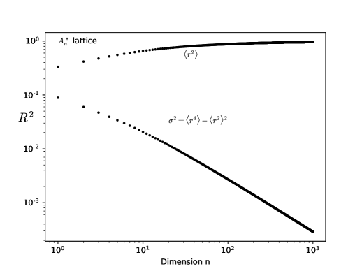
Figure 6: The mean and variance of the squared radius for the $A_{n}^{*}$ lattice for dimensions from 1 to 1000, obtained exactly using the recursion in Appendix B. At large dimension the distribution is a narrow peak at the squared WS radius $R^{2}$.

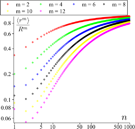
Figure 7: The even moments $\langle r^{m}\rangle$ for $m=2,4,6,8,10,12$ in the units of $R^{m}$ for the $A_{n}^{*}$ lattice for dimensions from 1 to 1000 are shown in the ascending order.

It is straightforward to study the distribution function numerically. First, select points at random from within the FP, by drawing the lattice coordinates $y_{1},\cdots,y_{n}$ from independent uniform distribution in the range $[0,\ell]$. Then identify the closest lattice point to $x=y_{i}{\mbox{\boldmath$e$}}_{i}$ and calculate the distance between the two. We now describe how to identify this closest lattice point. (An algorithm is given in Conway for $A_{n}$ as well as the correspondence with the dual lattice $A_{n}^{*}$, but we were unable to implement it.)

It is straightforward to show that the closest lattice point to $x$ must be one of the vertices of the FP. Since there are $2^{n}$ such vertices, when $n$ is large, it’s not computationally feasible to check the distances to all of them. However, it is trivial to show that the distance to the closest lattice point is unchanged if we permute the ordering of the lattice coordinates $y_{i}$. So the first step of simplification is to reorder the lattice coordinate values of $y_{i}$ in increasing order.

We now prove the following. If $0\leq y_{1}\leq\cdots\leq y_{n}\leq\ell$ are the lattice coordinates of a point in the FP, then the closest FP vertex has coordinates of the form $(0,\cdots,0,\ell,\cdots,\ell)$, where there are $k$ zeros followed by $(n-k)$ $\ell$’s. The proof is by contradiction.

Suppose that the closest vertex to the point with lattice coordinates $(y_{1},\cdots,y_{n})$ is a point with lattice coordinates $A=(0,\cdots,0,\ell,0,\ell,\cdots,\ell)$ and is at squared distance $r_{A}^{2}$. We use $y_{R}$ to denote the lattice coordinate value at the position of the rightmost zero, and $y_{L}$ to denote the value at the leftmost $\ell$. Now, construct a different lattice vertex B, by swapping the leftmost $\ell$ with the $0$ just to its right, so that $B=(0,\cdots,0,\ell,\ell,\cdots,\ell)$, and denote its squared distance from $y$ by $r_{B}^{2}$. The difference between the squared distances is

$$r_{A}^{2}-r_{B}^{2} = \left(1+\frac{1}{n}\right)\biggl{(}(y_{L}-\ell)^{2}+y_{R}^{2}-(y_{R}-\ell)^{2}-y_{L}^{2})\biggr{)}$$ (42)

$$= 2\ell\left(1+\frac{1}{n}\right)(y_{R}-y_{L}).$$

Since the coordinates are ordered so that $y_{L}<y_{R}$, it follows that $r_{A}^{2}-r_{B}^{2}>0$ and thus that $A$ is not the closest lattice vertex to $y$. The same argument shows that swapping a leftmost $\ell$ with a $0$ anywhere to its right will always decrease the distance. The result follows by induction.

This makes it computationally straightforward to identify the closest vertex to any point inside the FP. First, sort the lattice coordinates in increasing order. Then, calculate the distances to the $n+1$ vertices with coordinates of the form $(0,\cdots,0,\ell,\cdots,\ell)$ and select the minimum.

We have used this method to find $P_{r^{2}}(r^{2})$ numerically for the $A_{n}^{*}$ lattice, for dimensions from $n=1$ to $n=1000$. This is plotted in Fig. 5. In comparison with the cubic lattice $\mathbb{Z}^{n}$, two differences are immediately apparent. The first is that as the dimension $n$ increases, the distribution increasingly becomes peaked around the WS radius $R$, and the second is that the Gaussian approximation (with the correct mean and variance) is not good, because it does not fall off fast enough as $r\to R$.

VII Conclusion

In this paper, we have computed and compared the loss fractions of two template grids. The first is based on the simple cubic lattice $\mathbb{Z}^{n}$, and the second is based on the root lattice $A_{n}^{*}$, which is a generalization of the two-dimensional hexagonal lattice. In particular, we extend the results of NewAllenPaper to the case of large mismatch, by exploiting the spherical approximation AllenSpherical .

The main result is rather clear, and visible in the upper part of Fig. 4. The slight advantages offered by the $A_{n}^{*}$ lattice at small mismatch decrease at larger mismatch. This can be easily understood from the distribution of the squared radius for points randomly selected within the Wigner-Seitz (WS) cell. As the dimension $n$ of parameter space increases, this distribution becomes an increasingly narrow peak centered closer and closer to the squared WS radius.

We believe that this behavior may be general, and true for any lattice in the limit as the dimension $n\to\infty$. To state it precisely, the distribution function for the squared radius becomes an increasingly narrow peak, which is true if and only if

$$\lim_{n\to\infty}\langle r^{2m}\rangle=\langle r^{2}\rangle^{m},$$ (43)

with the understanding that the WS radius $R$ is held fixed during the limiting process. We have tried to prove this using Jensen’s inequality Perlman , but are not convinced that our argument is correct.

The final messages for the data analyst are simple ones. First, a fairly effective template-based search can be constructed at mismatch values that are shockingly high in the quadratic approximation (quadratic mismatch exceeding unity!). Second, if the goal is to detect as many signals as possible at fixed computing cost, there is little motivation for using template banks based on sophisticated lattices such as $A_{n}^{*}$. These offer only minimal benefit when compared with the humble cubic lattice $\mathbb{Z}^{n}$, and that minor advantage diminishes as the template separation increases.

VIII Acknowledgments

We thank Mathieu Dutour Sikirić for bringing the thinnest known lattices of Sikiric_2008 to our attention.

Appendix A Even moments of the $\mathbb{Z}^{n}$ lattice

For the $\mathbb{Z}^{n}$ lattice, the general even-order moment can be computed as follows. One uses the multinomial expansion to write

$$\langle r^{2m}\rangle=\sum_{k_{1}+\cdots+k_{n}=m}\binom{m}{k_{1},\cdots,k_{n}}\prod_{i=1}^{n}\langle x_{i}^{2k_{i}}\rangle,$$ (44)

where the sum is over all non-negative integer $k_{i}$ whose sum equals $m$. The multinomial coefficient is

$$\binom{m}{k_{1},k_{2},\cdots,k_{n}}=\frac{m!}{k_{1}!k_{2}!\cdots k_{n}!},$$ (45)

and the coordinate moments are

$$\langle x^{2k}\rangle=\frac{1}{\ell}\int_{-\ell/2}^{\ell/2}x^{2k}dx=\frac{1}{2k+1}\left(\frac{\ell}{2}\right)^{2k}.$$ (46)

In the sum Eq. (44), there are many identical terms on the r.h.s. which are obtained by permutation of the indices of the $k_{i}$. The number of these identical terms depends upon the number of distinct non-zero values taken by the $k_{i}$, which in turn depends upon the dimension $n$.

Suppose that for each term, the non-zero $k_{i}$ are sorted in increasing order; there at most $m$ of them. Let $q\leq m$ denote the number of these non-zero $k_{i}$, and let $n_{1}$ denote the number of $k_{i}$ which have the smallest value, $n_{2}$ the next smallest, and so on; the sum is bounded by $\sum_{i}n_{i}\leq m$. Then the number of equivalent (under permutation) terms which appear on the r.h.s. of Eq. (44) is equal to the number of ways in which $n_{1}$ coordinates can be chosen from the $n$, and $n_{2}$ can be chosen from the remaining $n-n_{1}$, and so on. This is

$$N(k_{1},\cdots,k_{q})$$ (47)

$$= \binom{n}{n_{1}}\binom{n-n_{1}}{n_{2}}\times\cdots\times\binom{n-n_{1}-\cdots-n_{p-1}}{n_{p}}$$

$$= \frac{n!}{n_{1}!n_{2}!\cdots n_{p}!(n-n_{1}-\cdots-n_{p})!},$$

where the quantities in the second line are the standard binomial (choice) coefficients; the r.h.s. is a polynomial in $n$ of order $\leq m$. Thus one obtains

$$\langle r^{2m}\rangle=\sum_{k_{1}+\cdots+k_{q}=m}\frac{\binom{m}{k_{1},\cdots,k_{q}}N(k_{1},\cdots,k_{q})}{(2k_{1}+1)\cdots(2k_{q}+1)}\left(\frac{\ell}{2}\right)^{2m}\,,$$ (48)

where the sum is over all distinct (under permutation) partitions $k_{i}$.

For example, for $m=5$, the r.h.s. of Eq. (48) has seven terms, with the following sets of $k_{i}$: $\{1,1,1,1,1\},\{1,1,1,2\},\{1,2,2\},\{1,1,3\},\{2,3\},\{1,4\}$, and $\{5\}$. Respectively, these have $n_{i}$ given by $\{5\},\{3,1\},\{1,2\},\{2,1\},\{1,1\},\{1,1\}$, and $\{1\}$, with corresponding $N$ given by $n(n-1)(n-2)(n-3)(n-4)/5!$, $n(n-1)(n-2)(n-3)/3!$, $n(n-1)(n-2)/2!$, $n(n-1)(n-2)/2!$, $n(n-1)$, $n(n-1)$ and $n$. Thus one obtains

$$\left(\frac{\ell}{2}\right)^{-10}\langle r^{10}\rangle=$$

$$\binom{5}{1,1,1,1,1}\frac{n(n-1)(n-2)(n-3)(n-4)}{5!\,3^{5}}+$$

$$\binom{5}{1,1,1,2}\frac{n(n-1)(n-2)(n-3)}{3!\,3^{3}5}+$$

$$\binom{5}{1,2,2}\frac{n(n-1)(n-2)}{2!\,5^{2}\,3}+\binom{5}{1,1,3}\frac{n(n-1)(n-2)}{2!\,3^{2}\,7}+$$

$$\binom{5}{2,3}\frac{n(n-1)}{5\cdot 7}+\binom{5}{1,4}\frac{n(n-1)}{3\cdot 9}+\binom{5}{5}\frac{n}{11}\,.$$

This simplifies, to give the tenth moment of Eq. (III).

The supplementary materials for this manuscript include a short Mathematica script to calculate arbitrary even moments of the $\mathbb{Z}^{n}$ lattice.

Appendix B Even moments of the $A_{n}^{*}$ lattice

Here we give a general expression for computation of any even moment of the $A_{n}^{*}$ lattice. The computation technique is a generalization of Chapter 21 Section 3.F of Conway , where it is used to find the second moment.

The un-normalized and normalized $p$’th moments of a region or object $D$ are defined as

$$U_{p}(D)=\int_{D}r^{p}dV,\text{ and }I_{p}(D)=U_{p}(D)/U_{0}(D),$$ (49)

where $D$ is the domain of integration and the radius $r$ is measured from the origin $O$ (see Fig. 8).

The WS cell in dimension $n$ is called a permutohedron and is denoted $P_{n}$. It has a complex shape with $(n+1)!$ vertices and $2^{n+1}-2$ faces. According to the definition Eq. (49), $U_{0}(P_{n})$ is the volume of the WS cell $P_{n}$. The normalized $m$’th moment $I_{p}(P_{n})$ is obtained by dividing out the volume.

Note that the length conventions used in this Appendix follow Conway , and differ from the conventions used in the remainder of this paper. To transform a quantity associated with $P_{n}$ with dimensions of length^d in this Section into the units used in the remainder of the paper, multiply by

$$\biggl{[}\frac{\ell^{2}}{n(n+1)}\biggr{]}^{d/2}.$$ (50)

For example, in the conventions of this Section, the point in $P_{n}$ most distant from the center has squared radius $n(n+1)(n+2)/12$, which should be compared with Eq. (18), and the volume is $U_{0}(P_{n})=(n+1)^{n-1/2}$, which should be compared with Eq. (14).

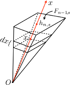
Figure 8: The $n$-dimensional pyramid associated with $(n-1)$-dimensional face $F_{n-1,s}$. The point $O$ is such that for all congruent faces $F_{n-1,s}$ the associated pyramids are congruent. The axis $Ox$ is perpendicular to the face $F_{n-1,s}$, and $h_{n-1,s}$ is the distance form $O$ to the face. The increment $dx$ is thickness of the slab at $x$.

Each face of $P_{n}$ is the direct product of a pair of lower-dimensional permutohedrons . For $n$ even there are $n/2$ types of faces and for $n$ odd there are $(n+1)/2$ types of faces. Following Conway the different types of faces are labeled by $s=0,\cdots,n-1$. A face of type $s$, $F_{n-1,s}$, is the Cartesian product, $F_{n-1,s}=P_{s}\times P_{n-s-1}$; faces of type $s$ and faces of type $n-s-1$ are equivalent. The number of faces of type $s$ is the binomial coefficient

$${{n+1}\choose{s+1}}.$$ (51)

The squared distance from the center of $P_{n}$ to the center of a face of type $s$ is

$$h^{2}_{n,s}=\frac{1}{4}(s+1)(n-s)(n+1).$$ (52)

By symmetry, the line from the center of $P_{n}$ to the center of any face is orthogonal to the face. We call this the center line to the face.

Because the faces are formed from lower-dimensional permutohedrons, the moments may be calculated by recursion. We divide $P_{n}$ into generalized pyramids, one face at a time, by taking the bundle of all line segments that begin at the center of the $P_{n}$ and extend to anywhere in that face. These pyramids are disjoint (apart from a set of measure zero on their boundaries) and their union is $P_{n}$. To compute the moments of $P_{n}$, we compute the moments of the pyramids and sum them.

The $m$’th moment of each pyramid can be found with elementary calculus. We slice each pyramid into slabs of thickness $dx$, where $x\in[0,h_{n,s}]$ is a a coordinate that runs along the center line to a face of type $s$, and the slicing is orthogonal to the center line shown in Fig. 8. Each slab has $n$-volume

$$dV=\frac{x^{n-1}}{h_{n,s}^{n-1}}U_{0}(P_{s})U_{0}(P_{n-s-1})dx,$$ (53)

so by integration over $x$ the volume of the pyramid is

$$\int^{h_{n,s}}_{0}dV=\frac{1}{n}h_{n,s}U_{0}(P_{s})U_{0}(P_{n-s-1}).$$ (54)

Summing over all faces gives

$$U_{0}(P_{n})={1\over n}\sum_{s=0}^{n-1}{{n+1}\choose{s+1}}h_{n,s}U_{0}(P_{s})U_{0}(P_{n-s-1}).$$ (55)

This recursion relation, together with the initial value $U_{0}(P_{0})=1$, determines the volume $U_{0}(P_{n})$ for dimensions $n>0$.

To construct a general recursion relation for an arbitrary even moment $U_{2m}(P_{n})$, $m=0,1,2,3,...$, we begin with the expression

$$U_{2m}(P_{n})=\sum_{s=0}^{n-1}{{n+1}\choose{s+1}}U_{2m}(P_{n,s})\,,$$ (56)

where $U_{2m}(P_{n,s})$’s are the moments of $n$-dimensional pyramids $P_{n,s}$ into which a permutohedron $P_{n}$ is decomposed. Every such moment can be calculated by using the definition Eq. (49), substituting for $r^{2}$ the expression

$$r^{2}=\frac{x^{2}}{h^{2}_{n,s}}\rho^{2}_{n-1,s}+x^{2}\,,$$ (57)

where $\rho_{n-1,s}$ is the distance from the point of intersection of the axis $Ox$ with the face $F_{n-1,s}$ to arbitrary point of the face (see Fig. 8), as follows:

$$U_{2m}(P_{n,s}) = \int_{F_{n-1,s}}dV\,\int^{h_{n,s}}_{0}dx\,\left(\frac{x^{2}}{h^{2}_{n,s}}\rho^{2}_{n-1,s}+x^{2}\right)^{m}$$

$$= \sum_{k=0}^{m}{{m}\choose{k}}\int_{F_{n-1,s}}\rho^{2k}_{n-1,s}dV\int^{h_{n,s}}_{0}\frac{x^{2m+n-1}}{h_{n,s}^{n-1+2k}}dx\,,$$

where the volume element $dV$ is in the face $F_{n-1,s}$. (For odd moments $m=k+1/2$, where $k=0,1,2,...$ the finite sum in the expression above is replaced by an infinite series.) Using the definition Eq. (49) for the moments $U_{2k}(F_{n-1,s})$ of faces $F_{n-1,s}$ (here, with origin at the center of the face) and integrating over $x$ we obtain

$$U_{2m}(P_{n,s})=\frac{h_{n,s}^{2(m-k)+1}}{n+2m}\sum_{k=0}^{m}{{m}\choose{k}}U_{2k}(F_{n-1,s})\,.$$ (58)

Substituting this expression into Eq. (56) we obtain

$$U_{2m}(P_{n}) = {1\over n+2m}\sum_{s=0}^{n-1}\sum_{k=0}^{m}{{n+1}\choose{s+1}}{{m}\choose{k}}$$ (59)

$$\times h_{n,s}^{2(m-k)+1}U_{2k}(F_{n-1,s})\,.$$

The next step is to consider the face $F_{n-1,s}$ as the Cartesian product $P_{s}\times P_{n-s-1}$ and apply again the definition Eq. (49) to the moments $U_{2k}(F_{n-1,s})$, with the origin at the center of the face. Replace $r^{2}$ with

$$\rho^{2}_{n-1,s}=\rho^{2}_{s}+\rho^{2}_{n-1-s}\,,$$ (60)

and use the binomial theorem to raise Eq. (60) to power $k$. Employing the definition Eq. (49) for the moments $U_{2j}(P_{s})$ and $U_{2(k-j)}(P_{n-1-s})$, we obtain

$$U_{2k}(F_{n-1,s})=\sum_{j=0}^{k}{{k}\choose{j}}U_{2j}(P_{s})U_{2(k-j)}(P_{n-s-1})\,.$$ (61)

Finally, substituting Eq. (61) into Eq. (59), we obtain the following relation for the even moments of $P_{n}$:

$$U_{2m}(P_{n}) = {1\over n+2m}\sum_{s=0}^{n-1}\sum_{k=0}^{m}\sum_{j=0}^{k}{{n+1}\choose{s+1}}{{m}\choose{k}}{{k}\choose{j}}$$ (62)

$$\times h^{2(m-k)+1}_{n,s}U_{2j}(P_{s})U_{2(k-j)}(P_{n-s-1})\,.$$

This recursion relation, together with the initial values $U_{0}(P_{0})=1$ and $U_{2m}(P_{0})=0$, for $m=1,2,3,...$, defines an arbitrary even-order moment.

In Tables 2 and 3 we give numerical and exact values for the even moments $\langle r^{2m}\rangle$ obtained from $U_{2m}(P_{n})$, for dimensions $n<16$. The un-normalized moments are computed using the recursion relation Eq. (62). The normalized moments $I_{2m}(P_{n})$ are then defined by 49. Both of these follow the conventions of Conway and Sloane, Chapter 21 Section 3F Conway . They are then re-scaled following Eq. (50) with $d=2m$ to obtain $\langle r^{2m}\rangle$, which are in the conventions used everywhere else in this paper.

The following lines of Mathematica are sufficient to calculate the arbitrary even moments $U_{2m}(P_{n})={\rm U[m,n]}$ up to dimensions of several thousand. The normalized moments are $I_{2m}(P_{n})={\rm II[m,n]}$, and the moments (with the length conventions used in the remainder of this paper, as they appear in Tables 2 and 3) are $<r^{2m}>={\rm Mo[m,n]}$.

     h[n_,s_]:= h[n,s] = Sqrt[(s+1)(n-s)(n+1)]/2  U[m_,0 ]:= U[m,0] = If[m==0, 1, 0]  U[m_,n_]:= U[m,n] = Simplify[Sum[   Binomial[n+1,s+1] Binomial[m,k] Binomial[k,j]   h[n,s]^(2 m - 2 k + 1) U[j, s] U[k-j, n-s-1],  {s, 0, n-1},{k, 0, m},{j, 0, k}]/(n+2 m)]  II[m_,n_]:=U[m,n]/U[0,n]  Mo[m_,n_]:=II[m,n](12 R^2/(n(n+1)(n+2)))^m     

$n$	$\langle r^{2}\rangle/R^{2}$	$\langle r^{4}\rangle/R^{4}$	$\langle r^{6}\rangle/R^{6}$	$\langle r^{8}\rangle/R^{8}$	$\langle r^{10}\rangle/R^{10}$	$\langle r^{12}\rangle/R^{12}$
$1$	$0.3333$	$0.2000$	$0.1429$	$0.1111$	$0.0909$	$0.0769$
$2$	$0.4167$	$0.2333$	$0.1482$	$0.1013$	$0.0727$	$0.0541$
$3$	$0.4750$	$0.2727$	$0.1728$	$0.1167$	$0.0824$	$0.0602$
$4$	$0.5187$	$0.3083$	$0.1987$	$0.1353$	$0.0959$	$0.0701$
$5$	$0.5529$	$0.3397$	$0.2233$	$0.1540$	$0.1101$	$0.0810$
$6$	$0.5807$	$0.3672$	$0.2460$	$0.1720$	$0.1242$	$0.0921$
$7$	$0.6038$	$0.3914$	$0.2669$	$0.1891$	$0.1380$	$0.1031$
$8$	$0.6234$	$0.4130$	$0.2862$	$0.2052$	$0.1512$	$0.1139$
$9$	$0.6404$	$0.4324$	$0.3039$	$0.2204$	$0.1639$	$0.1244$
$10$	$0.6552$	$0.4499$	$0.3202$	$0.2346$	$0.1760$	$0.1346$
$11$	$0.6683$	$0.4657$	$0.3354$	$0.2481$	$0.1876$	$0.1444$
$12$	$0.6800$	$0.4802$	$0.3496$	$0.2608$	$0.1986$	$0.1539$
$13$	$0.6905$	$0.4936$	$0.3628$	$0.2728$	$0.2092$	$0.1630$
$14$	$0.7001$	$0.5058$	$0.3751$	$0.2842$	$0.2193$	$0.1719$
$15$	$0.7088$	$0.5172$	$0.3867$	$0.2950$	$0.2290$	$0.1804$

Table 2: Numerical values for the first six even moments of the WS cell $P_{n}$ of the $A_{n}^{*}$ lattice for dimensions $n=1,\dots,15$, where the covering radius $R$ is given in Eq. (18). The exact values of these moments are given in Table 3. In the text we argue that $\lim_{n\to\infty}\langle r^{2}\rangle/R^{2}=1$, and that $\lim_{n\to\infty}\langle r^{2}m\rangle=\langle r^{2}\rangle^{m}$. Hence, as $n\to\infty$, all of these table entries should approach unity.

Table 3: Exact values of the lowest-order even moments for the $A_{n}^{*}$ lattice, as given by the recursion relationship derived in Appendix B. Numerical values may be found in Table 2.

$n$	$\langle r^{2}\rangle/R^{2}$	$\langle r^{4}\rangle/R^{4}$	$\langle r^{6}\rangle/R^{6}$	$\langle r^{8}\rangle/R^{8}$	$\langle r^{10}\rangle/R^{10}$	$\langle r^{12}\rangle/R^{12}$
$1$	$\frac{1}{3}$	$\frac{1}{5}$	$\frac{1}{7}$	$\frac{1}{9}$	$\frac{1}{11}$	$\frac{1}{13}$
$2$	$\frac{5}{12}$	$\frac{7}{30}$	$\frac{83}{560}$	$\frac{319}{3150}$	$\frac{403}{5544}$	$\frac{1517}{28028}$
$3$	$\frac{19}{40}$	$\frac{409}{1500}$	$\frac{27217}{157500}$	$\frac{38281}{328125}$	$\frac{1427333}{17325000}$	$\frac{539235971}{8957812500}$
$4$	$\frac{389}{750}$	$\frac{37}{120}$	$\frac{312953}{1575000}$	$\frac{15977293}{118125000}$	$\frac{41514229}{433125000}$	$\frac{10041681373}{143325000000}$
$5$	$\frac{209}{378}$	$\frac{22469}{66150}$	$\frac{1085536}{4862025}$	$\frac{131002604}{850854375}$	$\frac{43271601607}{393094721250}$	$\frac{120676030448681}{1490484151406250}$
$6$	$\frac{78077}{134456}$	$\frac{423151}{1152480}$	$\frac{66683227}{271063296}$	$\frac{2855332489}{16602626880}$	$\frac{3049146605765}{24545323579392}$	$\frac{561024599680723}{6091703033794560}$
$7$	$\frac{89035}{147456}$	$\frac{1515163}{3870720}$	$\frac{3645004793}{13655900160}$	$\frac{813284979379}{4301608550400}$	$\frac{43871720179117}{317974904045568}$	$\frac{47003442367289761}{455737531223310336}$
$8$	$\frac{3313213}{5314410}$	$\frac{146336671}{354294000}$	$\frac{127738979843}{446410440000}$	$\frac{23552471440009}{114791256000000}$	$\frac{343658283760349}{2272866868800000}$	$\frac{26512131817729691533}{232684745693400000000}$
$9$	$\frac{1100657}{1718750}$	$\frac{117719}{272250}$	$\frac{895784540747}{2947957031250}$	$\frac{535892016104111}{2432064550781250}$	$\frac{217007542831819286}{1324259147900390625}$	$\frac{7422858954915606122659}{59651253317173095703125}$
$10$	$\frac{18539106101}{28295372292}$	$\frac{9643229133}{21435888100}$	$\frac{396436661186}{1237922537775}$	$\frac{7667873302060633}{32681154997260000}$	$\frac{556729110272163449}{3163535803734768000}$	$\frac{4395579391379571244226791}{32656586938990809795000000}$
$11$	$\frac{25941989}{38817792}$	$\frac{6463162733}{13877360640}$	$\frac{1863816574691}{5556495200256}$	$\frac{1400046042361}{5643315437760}$	$\frac{1406514743813641321}{7499234843102306304}$	$\frac{26425247449515274378841}{182976643149919334876160}$
$12$	$\frac{17061288862565}{25090245516518}$	$\frac{389281868476643}{810607932072120}$	$\frac{135373127776116799}{387267939547455330}$	$\frac{3186173305108287135529}{12217012599590390810400}$	$\frac{194307923663053340412317}{978338368975198496096832}$	$\frac{44840145568064414926573819}{291366954251159115746656512}$
$13$	$\frac{81923134171}{118639604580}$	$\frac{2718612928907}{5508267355500}$	$\frac{4772968402612073}{13157873645450625}$	$\frac{26384102217284296859}{96710371294062093750}$	$\frac{8775008810370829285906}{41949735388321000865625}$	$\frac{3034165287365868825626600411}{18609951361643904009012890625}$
$14$	$\frac{3588341852791}{5125781250000}$	$\frac{5807913344549}{11481750000000}$	$\frac{6330843027118853801}{16878172500000000000}$	$\frac{3357739197420742084967}{11814720750000000000000}$	$\frac{9575820529342227197910377}{43667207892000000000000000}$	$\frac{17383801168332194619594087887}{101149132462560000000000000000}$
$15$	$\frac{423929152911307}{598134325510144}$	$\frac{49305729309609649}{95327658128179200}$	$\frac{210551088639050555933}{544511583228159590400}$	$\frac{19505342217281370335341}{66119263677705093120000}$	$\frac{271786289285385309816213443}{1186973021542161831690240000}$	$\frac{664211366929553172581639942783}{3682314032738752046039040000000}$

References

- (1) L. A. Wainstein and V. D. Zubakov, “Extraction of Signals from Noise”, Dover (1970).
- (2) C. W. Helstrom, “Statistical Theory of Signal Detection”, International series of monographs on electronics and instrumentation, Pergamon Press (1960).
- (3) B. F. Schutz, “Gravitational Wave Sources and Their Detectability,” Class. Quant. Grav. 6, 1761-1780 (1989).
- (4) B. S. Sathyaprakash and S. V. Dhurandhar, “Choice of filters for the detection of gravitational waves from coalescing binaries,” Phys. Rev. D 44, 3819-3834 (1991).
- (5) B. F. Schutz, in The Detection of Gravitational Waves, edited by D. G. Blair (1991) p. 406.
- (6) C. Cutler, T. A. Apostolatos, L. Bildsten, L. S. Finn, E. E. Flanagan, D. Kennefick, D. M. Markovic, A. Ori, E. Poisson and G. J. Sussman, et al. “The Last three minutes: issues in gravitational wave measurements of coalescing compact binaries,” Phys. Rev. Lett. 70, 2984-2987 (1993); [arXiv:astro-ph/9208005 [astro-ph]].
- (7) B. S. Sathyaprakash, “Filtering post-Newtonian gravitational waves from coalescing binaries,” Phys. Rev. D 50, no.12, 7111-7115 (1994); [arXiv:gr-qc/9411043 [gr-qc]].
- (8) C. Cutler and E. E. Flanagan, “Gravitational waves from merging compact binaries: How accurately can one extract the binary’s parameters from the inspiral wave form?,” Phys. Rev. D 49, 2658-2697 (1994); [arXiv:gr-qc/9402014 [gr-qc]].
- (9) S. V. Dhurandhar and B. S. Sathyaprakash, “Choice of filters for the detection of gravitational waves from coalescing binaries. 2. Detection in colored noise,” Phys. Rev. D 49, 1707-1722 (1994);
- (10) S. V. Dhurandhar and B. F. Schutz, “Filtering coalescing binary signals: Issues concerning narrow banding, thresholds, and optimal sampling,” Phys. Rev. D 50, 2390-2405 (1994).
- (11) R. Balasubramanian and S. V. Dhurandhar, “Performance of Newtonian filters in detecting gravitational waves from coalescing binaries,” Phys. Rev. D 50, 6080-6088 (1994); [arXiv:gr-qc/9404009 [gr-qc]].
- (12) R. Balasubramanian, B. S. Sathyaprakash and S. V. Dhurandhar, “Gravitational waves from coalescing binaries: Detection strategies and Monte Carlo estimation of parameters,” Phys. Rev. D 53, 3033-3055 (1996); [erratum: Phys. Rev. D 54, 1860 (1996)]; [arXiv:gr-qc/9508011 [gr-qc]].
- (13) B. J. Owen and B. S. Sathyaprakash, “Matched filtering of gravitational waves from inspiraling compact binaries: Computational cost and template placement,” Phys. Rev. D 60, 022002 (1999); [arXiv:gr-qc/9808076 [gr-qc]].
- (14) B. Allen, W. G. Anderson, P. R. Brady, D .A. Brown, and J. D. E. Creighton, “FINDCHIRP: An algorithm for detection of gravitational waves from inspiraling compact binaries,” Phys. Rev. D 85, 122006 (2012).
- (15) L. Nieder and B. Allen and C. J. Clark and H. J. Pletsch , “Exploiting Orbital Constraints from Optical Data to Detect Binary Gamma-Ray Pulsars”, ApJ 901/2, p.156 (2020).
- (16) B. P. Abbott et al. (LIGO Scientific Collaboration and Virgo Collaboration), “First low-frequency Einstein@Home all-sky search for continuous gravitational waves in Advanced LIGO data”, Phys. Rev. D 96, 122004 (2017).
- (17) C. Messenger, R. Prix and M. A. Papa, “Random template banks and relaxed lattice coverings,” Phys. Rev. D 79, 104017 (2009); [arXiv:0809.5223 [gr-qc]].
- (18) I. W. Harry, B. Allen and B. S. Sathyaprakash, “A Stochastic template placement algorithm for gravitational wave data analysis,” Phys. Rev. D 80, 104014 (2009); [arXiv:0908.2090 [gr-qc]].
- (19) B. Allen, “Optimal Template Banks”, (2021); [arXiv:2102.11254 [astro-ph]].
- (20) Benjamin J. Owen, “Search templates for gravitational waves from inspiraling binaries: Choice of template spacing”, Phys. Rev. D 53, 6749 (1996).
- (21) B. Allen, “Spherical ansatz for parameter-space metrics”, Phys. Rev. D 100, 124004 (2019); [arXiv:arXiv:1906.01352 [gr-qc]].
- (22) J. H. Conway and N. J. A. Sloane, Sphere Packings, Lattices and Groups (Springer, Berlin, 1999).
- (23) R. Prix, Template-based searches for gravitational waves: efficient lattice covering of flat parameter spaces, Class. Quant. Grav. 24, S481-S490 (2007); [arXiv:0707.0428 [gr-qc]].
- (24) M. D. Sikirić, A. Schürmann, and F. Vallentin, A generalization of Voronoi’s reduction theory and its application, Duke Mathematical Journal 142, 127 (2008).
- (25) S. S. Ryshkov and E. P. Baranovskii, “Solution of the Problem of Least Dense Lattice Covering of Five-dimensional Space by Equal Spheres”, DAN 222, 39 (1975).
- (26) J. Mathews and R. L. Walker, Mathematical Methods of Physics, 2nd Edition, (Addison-Wesley, New York, 1970).
- (27) M. D. Perlman, “Jensen’s Inequality for a Convex Vector-valued Function on an Infinite-dimensional Space,” Journal of Multiplicative Analysis 4, 52 (1974).