Deep Deterministic Uncertainty: A Simple Baseline

Abstract

Reliable uncertainty from deterministic single-forward pass models is sought after because conventional methods of uncertainty quantification are computationally expensive. We take two complex single-forward-pass uncertainty approaches, DUQ and SNGP, and examine whether they mainly rely on a well-regularized feature space. Crucially, without using their more complex methods for estimating uncertainty, a single softmax neural net with such a feature-space, achieved via residual connections and spectral normalization, outperforms DUQ and SNGP’s epistemic uncertainty predictions using simple Gaussian Discriminant Analysis post-training as a separate feature-space density estimator—without fine-tuning on OoD data, feature ensembling, or input pre-procressing. This conceptually simple Deep Deterministic Uncertainty (DDU) baseline can also be used to disentangle aleatoric and epistemic uncertainty and performs as well as Deep Ensembles, the state-of-the art for uncertainty prediction, on several OoD benchmarks (CIFAR-10/100 vs SVHN/Tiny-ImageNet, ImageNet vs ImageNet-O) as well as in active learning settings across different model architectures, yet is computationally cheaper.

1 Introduction

Two types of uncertainty are often of interest in ML: epistemic uncertainty, which is inherent to the model, caused by a lack of training data, and hence reducible with more data, and aleatoric uncertainty, caused by inherent noise or ambiguity in data, and hence irreducible with more data (Der Kiureghian & Ditlevsen, 2009). Disentangling these two is critical for applications such as active learning (Gal et al., 2017) or detection of out-of-distribution (OoD) samples (Hendrycks & Gimpel, 2016): in active learning, we wish to avoid inputs with high aleatoric but low epistemic uncertainty, and in OoD detection, we wish to avoid mistaking ambiguous in-distribution (iD) examples as OoD. This is particularly challenging for noisy and ambiguous datasets found in safety-critical applications like autonomous driving (Huang & Chen, 2020) and medical diagnosis (Esteva et al., 2017; Filos et al., 2019).

Related Work. Most well-known methods of uncertainty quantification in deep learning (Blundell et al., 2015; Gal & Ghahramani, 2016; Lakshminarayanan et al., 2017; Wen et al., 2019; Dusenberry et al., 2020) require multiple forward passes at test time. Amongst these, Deep Ensembles have generally performed best in uncertainty prediction (Ovadia et al., 2019), but their significant memory and compute burden at training and test time hinders their adoption in real-life and mobile applications. Consequently, there has been an increased interest in uncertainty quantification using deterministic single forward-pass neural networks which have a smaller footprint and lower latency. Among these approaches, Lee et al. (2018b) uses Mahalanobis distances to quantify uncertainty by fitting a class-wise Gaussian distribution (with shared covariance matrices) on the feature space of a pre-trained ResNet encoder. They do not consider the structure of the underlying feature-space, which might explain why their competitive results require input perturbations, ensembling GMM densities from multiple layers, and fine-tuning on OoD hold-out data.

Table 1: OoD detection performance of different baselines using a Wide-ResNet-28-10 architecture with the CIFAR-10 vs SVHN/CIFAR-100/Tiny-ImageNet and CIFAR-100 vs SVHN/Tiny-ImageNet dataset pairs averaged over 25 runs. SN: Spectral Normalisation, JP: Jacobian Penalty. The best deterministic single-forward pass method and the best method overall are in bold for each metric.

Train Dataset	Method	Penalty	Aleatoric Uncertainty	Epistemic Uncertainty	Accuracy ($\uparrow$)	ECE ($\downarrow$)	AUROC SVHN ($\uparrow$)	AUROC CIFAR-100 ($\uparrow$)	AUROC Tiny-ImageNet ($\uparrow$)
CIFAR-10	Softmax	-	Softmax Entropy	Softmax Entropy	$95.98\pm 0.02$	$\mathbf{0.85\pm 0.02}$	$94.44\pm 0.43$	$89.39\pm 0.06$	$88.42\pm 0.05$
	Energy-based (Liu et al., 2020b)	-		Softmax Density			$94.56\pm 0.51$	$88.89\pm 0.07$	$88.11\pm 0.06$
	DUQ (van Amersfoort et al., 2020)	JP	Kernel Distance	Kernel Distance	$94.6\pm 0.16$	$1.55\pm 0.08$	$93.71\pm 0.61$	$85.92\pm 0.35$	$86.83\pm 0.12$
	SNGP (Liu et al., 2020a)	SN	Predictive Entropy	Predictive Entropy	$\mathbf{96.04\pm 0.09}$	$1.8\pm 0.1$	$94.0\pm 1.3$	$91.13\pm 0.15$	$89.97\pm 0.19$
	DDU (ours)	SN	Softmax Entropy	GMM Density	$95.97\pm 0.03$	$\mathbf{0.85\pm 0.04}$	$\mathbf{97.86\pm 0.19}$	$\mathbf{91.34\pm 0.04}$	$\mathbf{91.07\pm 0.05}$
	5-Ensemble	-	Predictive Entropy	Predictive Entropy	$\mathbf{96.59\pm 0.02}$	$\mathbf{0.76\pm 0.03}$	$97.73\pm 0.31$	$\mathbf{92.13\pm 0.02}$	$90.06\pm 0.03$
	(Lakshminarayanan et al., 2017)			Mutual Information			$97.18\pm 0.19$	$91.33\pm 0.03$	$90.90\pm 0.03$
					Accuracy ($\uparrow$)	ECE ($\downarrow$)	AUROC SVHN ($\uparrow$)		AUROC Tiny-ImageNet ($\uparrow$)
CIFAR-100	Softmax	-	Softmax Entropy	Softmax Entropy	$80.26\pm 0.06$	$4.62\pm 0.06$	$77.42\pm 0.57$		$81.53\pm 0.05$
	Energy-based (Liu et al., 2020b)	-		Softmax Density			$78\pm 0.63$		$81.33\pm 0.06$
	SNGP (Liu et al., 2020a)	SN	Predictive Entropy	Predictive Entropy	$80.00\pm 0.11$	$4.33\pm 0.01$	$85.71\pm 0.81$		$78.85\pm 0.43$
	DDU (ours)	SN	Softmax Entropy	GMM Density	$\mathbf{80.98\pm 0.06}$	$\mathbf{4.10\pm 0.08}$	$\mathbf{87.53\pm 0.62}$		$\mathbf{83.13\pm 0.06}$
	5-Ensemble	-	Predictive Entropy	Predictive Entropy	$\mathbf{82.79\pm 0.10}$	$\mathbf{3.32\pm 0.09}$	$79.54\pm 0.91$		$82.95\pm 0.09$
	(Lakshminarayanan et al., 2017)			Mutual Information			$77.00\pm 1.54$		$82.82\pm 0.04$

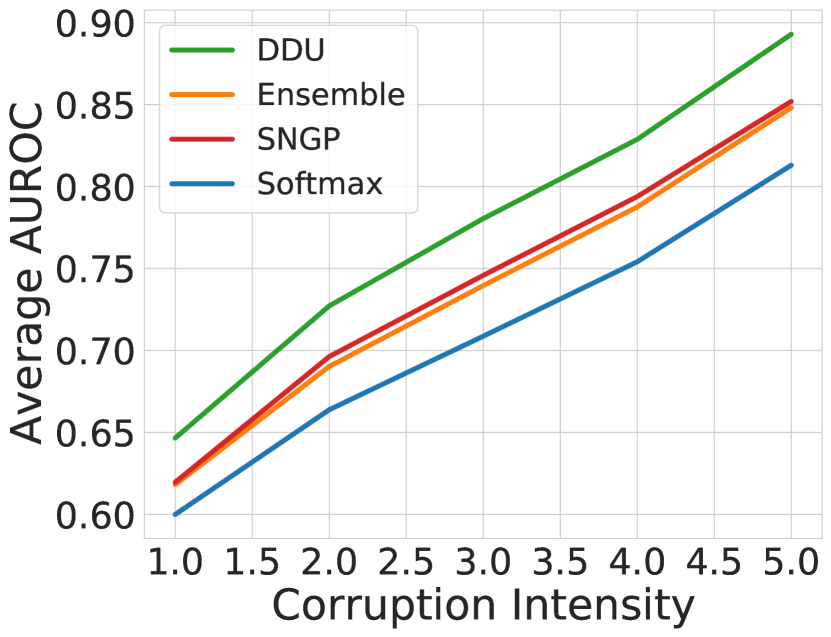
(a) Wide-ResNet-28-10

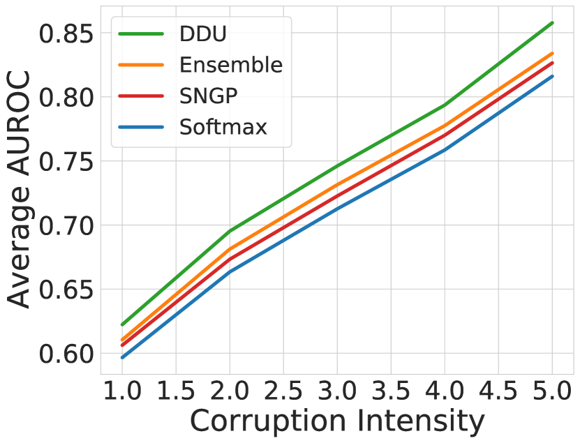
(b) ResNet-50

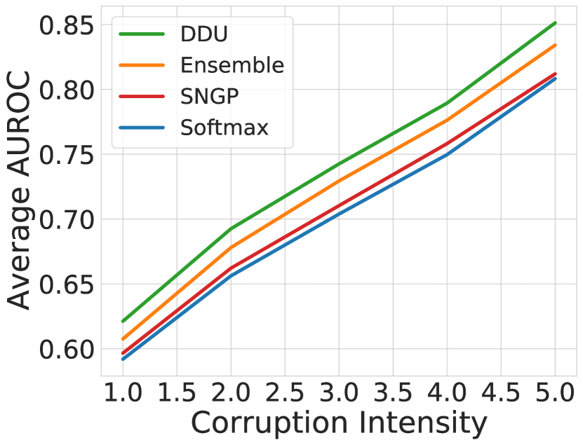
(c) ResNet-110

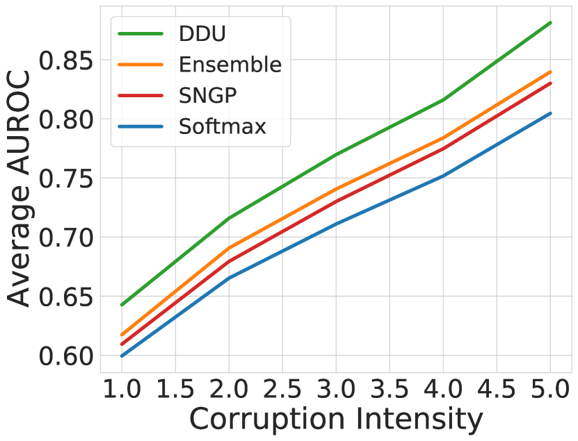
(d) DenseNet-121

Figure 1: AUROC vs corruption intensity averaged over all corruption types in CIFAR-10-C for architectures: Wide-ResNet-28-10, ResNet-50, ResNet-110 and DenseNet-121 and baselines: Softmax Entropy, Ensemble (using Predictive Entropy as uncertainty), SNGP, and DDU feature density. More details in §4.2 and more model architectures and ablations in §D in the appendix.

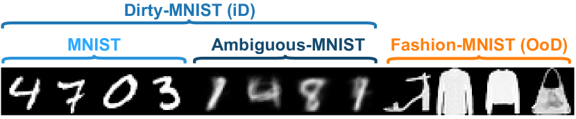
(a) Dirty-MNIST (iD) and Fashion-MNIST (OoD)

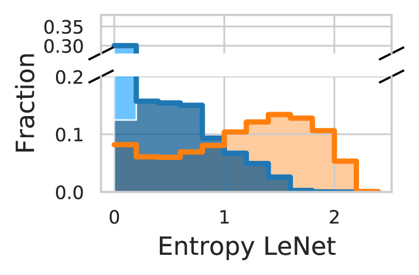
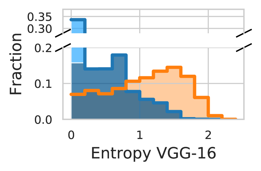
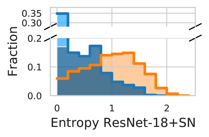
(b) Softmax entropy

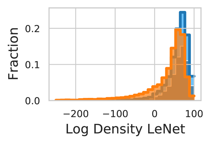
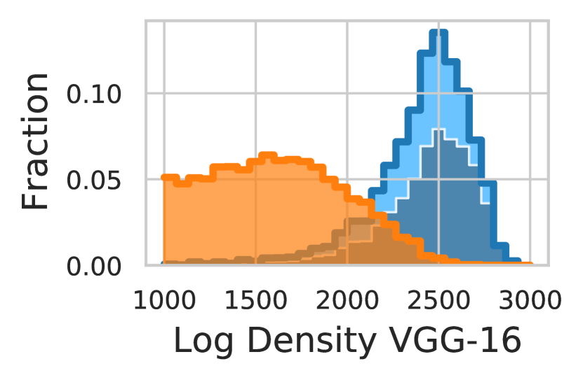
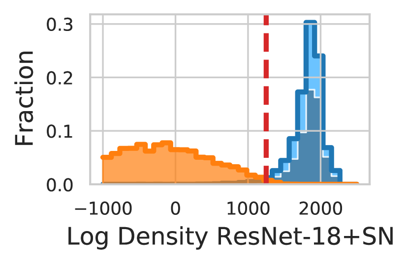
(c) Feature-space density

Figure 2: Disentangling aleatoric and epistemic uncertainty on Dirty-MNIST (iD) and Fashion-MNIST (OoD) 2(a) requires using softmax entropy 2(b) and feature-space density (GMM) 2(c) with a well-regularized feature space (ResNet-18+SN vs LeNet & VGG-16 without smoothness & sensitivity). 2(b): Softmax entropy captures aleatoric uncertainty for iD data (Dirty-MNIST), thereby separating unambiguous MNIST samples and Ambiguous-MNIST samples. However, iD and OoD are confounded: softmax entropy has arbitrary values for OoD, indistinguishable from iD. 2(c): With a well-regularized feature space (DDU with ResNet-18+SN), iD and OoD densities do not overlap, capturing epistemic uncertainty. However, without such feature space (LeNet & VGG-16), feature density suffers from feature collapse: iD and OoD densities overlap. Generally, feature-space density confounds unambiguous and ambiguous iD samples as their densities overlap.

DUQ & SNGP. Two recent works in single forward-pass uncertainty, DUQ (van Amersfoort et al., 2020) and SNGP (Liu et al., 2020a), propose distance-aware output layers, in the form of RBFs (radial basis functions) or GPs (Gaussian processes), and introduce additional inductive biases in the feature extractor using a Jacobian penalty (Gulrajani et al., 2017) or spectral normalisation (Miyato et al., 2018), respectively, which encourage smoothness and sensitivity in the latent space. These methods perform well and are almost competitive with Deep Ensembles on OoD benchmarks. However, they require training to be changed substantially, and introduce additional hyper-parameters due to the specialised output layers used at training. Furthermore, DUQ and SNGP cannot disentangle aleatoric and epistemic uncertainty. In DUQ, the feature representation of an ambiguous data point, high on aleatoric uncertainty, will be in between two centroids, but due to the exponential decay of the RBF it will seem far from both and thus have uncertainty similar to epistemically uncertain data points that are far from all centroids. In SNGP, the predictive variance is computed using a mean-field approximation of the softmax likelihood, which cannot be disentangled, or using MC samples of the softmax likelihood. In theory, the MC samples allow disentangling the uncertainty (see Equation 1), but this requires modelling the covariance between the classes, which is not the case in SNGP.

We provide a more extensive review of related work in §A.

Contributions. Firstly, we investigate the question whether complex methods to estimate uncertainty like in DUQ and SNGP are necessary beyond feature-space regularization that encourages bi-Lipschitzness. When we use spectral normalisation like SNGP does, the short answer is an empirical no. Indeed, with a well-regularized feature space using spectral normalisation, we find that we can fit a GDA after training, similar to Lee et al. (2018b), as feature-space density estimator to capture epistemic uncertainty—but, unlike Lee et al. (2018b), who do not place any constraints on the feature space, we do not require training on “OoD” hold-out data, feature ensembling, and input pre-processing to obtain good performance (see Table 1). The regularizing effect of spectral normalisation seems sufficient to not need these additional steps, resulting in a conceptually simpler method.

Secondly, we investigate how to disentangle aleatoric and epistemic uncertainty. This is something that DUQ and SNGP do not address directly. As we only fit GDA after training, the original softmax layer is trained using cross-entropy as a proper scoring rule (Gneiting & Raftery, 2007) and can be temperature-scaled to provide good in-distribution calibration and aleatoric uncertainty.

This combination of using GDA for epistemic uncertainty and the softmax predictive distribution for aleatoric uncertainty after training with feature-space regularisation, e.g. using spectral normalisation, provides a simple baseline which we call Deep Deterministic Uncertainty (DDU).

Altogether, DDU performs as well as a Deep Ensemble’s epistemic uncertainty (Lakshminarayanan et al., 2017) and outperforms SNGP and DUQ (van Amersfoort et al., 2020; Liu et al., 2020a) —with no changes to the model architecture beyond spectral normalisation—on several OoD benchmarks and active learning settings. It also outperforms regular softmax neural networks which might not capture epistemic uncertainty well, as illustrated in Figure 2.

Additional Insights. Beyond an empirical investigation and the description of DDU, we also provide several additional insights on potential pitfalls for practitioners. First, predictive entropy confounds aleatoric and epistemic uncertainty (Figure 2(b)). This can be an issue in active learning in particular. Yet, this issue is often not visible for standard benchmark datasets without aleatoric noise. To examine this failure in more detail, we introduce a new dataset, Dirty-MNIST, which showcases the issue more clearly than artificially curated datasets like MNIST or CIFAR-10. Dirty-MNIST is a modified version of MNIST (LeCun et al., 1998) with additional ambiguous digits (Ambiguous-MNIST) with multiple plausible labels and thus higher aleatoric uncertainty (Figure 2(a)). Secondly, the softmax entropy of a deterministic model, while being high for ambiguous points with high aleatoric uncertainty, might not be consistent for points with high epistemic uncertainty for models trained with maximum likelihood, i.e. the softmax entropy for the same OoD sample might be low, high or anything in between for different models trained on the same data (Figure 2(b)).

Feature-Space Regularization. Feature-space density can be a well-performing and simpler approach to estimate epistemic uncertainty (see Figure 2(c)). Crucially, the feature space needs to be well-regularized (Liu et al., 2020a): without smoothness and sensitivity, feature-space density alone might not separate iD from OoD data, possibly explaining the limited empirical success of previous approaches which attempt to use feature-space density (Postels et al., 2020). This can be seen in Figure 2(c) where the feature-space density of a VGG-16 or LeNet model are not able to differentiate iD Dirty-MNIST from OoD Fashion-MNIST while a ResNet-18 with spectral normalization can do so better.

Scope. Our focus is on obtaining a well-regularized feature space using spectral normalization in common model architectures with residual connections, following (Liu et al., 2020a). Unsupervised methods using contrastive learning (Winkens et al., 2020) might also obtain such a feature space by training on very large datasets, but access to them is generally limited or training on them very expensive (Sun et al., 2017). Similarly, we only use GDA for estimating the feature-space density as it is straight-forward to implement and does not require performing expectation maximization or variational inference like other density estimators. Normalizing flows (Dinh et al., 2015) or other more complex density estimators might provide even better density estimates, of course. However, GDA is a very simple method and already sufficient to outperform other more complex approaches and obtain good results. As the amount of training data available grows and feature extractors improve, the quality of feature representations might improve as well—an underlying hypothesis of this paper is that simple approaches will remain more applicable than more complex ones as our empirical results suggest.

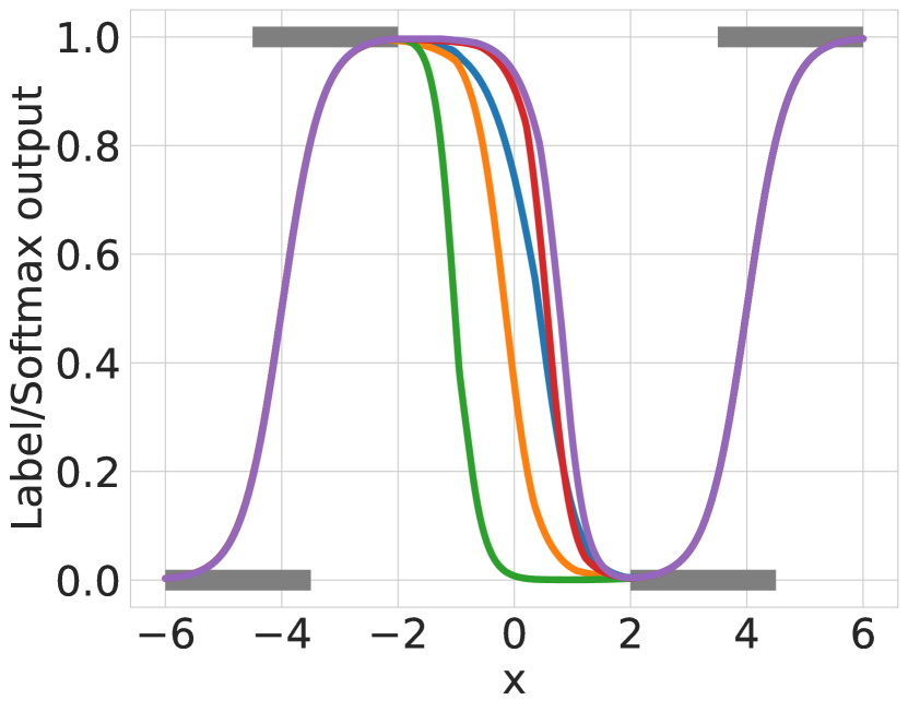
(a) Softmax output

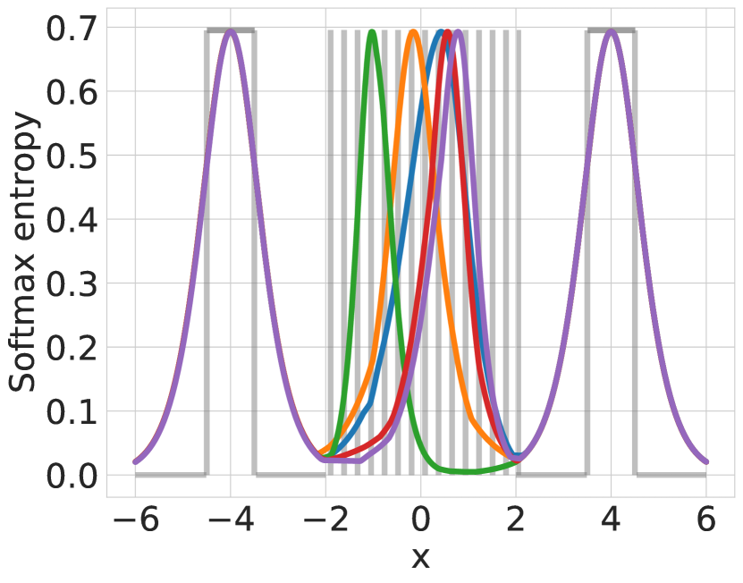
(b) Softmax entropy

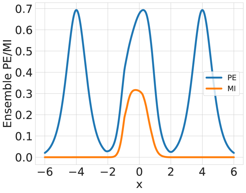
(c) 5-Ensemble

Figure 3: Softmax outputs & entropies for 5 softmax models along with the predictive entropy (PE) and mutual information (MI) for the resulting 5-Ensemble. 3(a) and 3(b) show that the softmax entropy is only reliably high for ambiguous iD points ($\pm$3.5–4.5), whereas it can be low or high for OoD points (-2–2). The different colors are the different ensemble components. Similarly, 3(c) shows that the MI of the ensemble is only high for OoD, whereas the PE is high for both OoD and for regions of ambiguity. See §F.4.

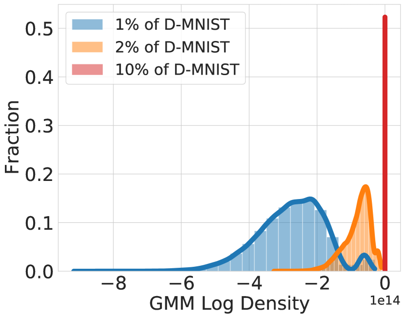
(d) Epistemic

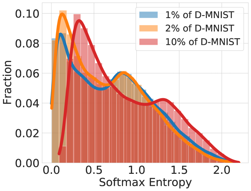
(e) Aleatoric

Figure 4: Epistemic and aleatoric uncertainty of ResNet-18+SN models trained on increasingly large subsets of DirtyMNIST. The feature-space density increases while the softmax entropy stays roughly the same, consistent with epistemic and aleatoric uncertainty being reducible and irreducible with more data, respectively. See §F.5 for a discussion on this.

2 Background

In this section, we review concepts important for quantifying uncertainty.

Epistemic Uncertainty at point $x$ is a quantity which is high for a previously unseen $x$, and decreases when $x$ is added to the training set and the model is updated (Kendall & Gal, 2017). This conforms with using mutual information in Bayesian models and deep ensembles (Kirsch et al., 2019) and feature-space density in deterministic models as surrogates for epistemic uncertainty (Postels et al., 2020) as we examine below—and depicted in Figure 3(d) (also §F.5).

Aleatoric Uncertainty at point $x$ is a quantity which is high for ambiguous or noisy samples (Kendall & Gal, 2017), i.e if multiple labels were to be observed at $x$, aleatoric will be high. It does not decrease with more data—depicted in Figure 3(e). Note that aleatoric uncertainty is only meaningful in-distribution, as, by definition, it quantifies the level of ambiguity between the different classes which might be observed for input $x$.

Bayesian Models (Neal, 2012; MacKay, 1992) provide a principled way of measuring uncertainty. Starting with a prior distribution $p(\omega)$ over model parameters $\omega$, they infer a posterior $p(\omega|\mathcal{D})$, given the training data $\mathcal{D}$. The predictive distribution $p(y|x,\mathcal{D})$ for a given input $x$ is computed via marginalisation over the posterior: $p(y|x,\mathcal{D})=\mathbb{E}_{\omega\sim p(\omega|\mathcal{D})}[p(y|x,\omega)]$. Its predictive entropy $\mathbb{H}[Y|x,\mathcal{D}]$ upper-bounds the epistemic uncertainty, where epistemic uncertainty is quantified as the mutual information $\mathbb{I}[Y;\omega|x,\mathcal{D}]$ (expected information gain) between parameters $\omega$ and output $y$ (Gal, 2016; Smith & Gal, 2018):

$$\underbrace{\mathbb{H}[Y|x,\mathcal{D}]}_{\text{predictive}}=\underbrace{\mathbb{I}[Y;\omega|x,\mathcal{D}]}_{\text{epistemic}}+\underbrace{\mathbb{E}_{\operatorname{p}(\omega\mathbin{|}\mathcal{D})}[\mathbb{H}[Y|x,\omega]]}_{\text{aleatoric (for iD $x$)}}.$$ (1)

Predictive uncertainty will be high whenever either epistemic uncertainty is high, or when aleatoric uncertainty is high. The intractability of exact Bayesian inference in deep learning has led to the development of methods for approximate inference (Hinton & Van Camp, 1993; Hernández-Lobato & Adams, 2015; Blundell et al., 2015; Gal & Ghahramani, 2016). In practice, however, these methods are either unable to scale to large datasets and model architectures, suffer from low uncertainty quality, or require expensive Monte-Carlo sampling.

Deep Ensembles are an ensemble of neural networks which average the models’ softmax outputs. Uncertainty is then estimated as the entropy of this averaged softmax vector. Despite incurring a high computational overhead at training and test time, Deep Ensembles, along with recent extensions (Smith & Gal, 2018; Wen et al., 2019; Dusenberry et al., 2020) form the state-of-the-art in uncertainty quantification in deep learning.

Deterministic Models produce a softmax distribution $p(y|x,\omega)$, and commonly either the softmax confidence $\max_{c}p(y=c|x,\omega)$ or the softmax entropy $\mathbb{H}[Y|x,\omega]$ are used as a measure of uncertainty (Hendrycks & Gimpel, 2016). Popular approaches to improve these metrics include pre-processing of inputs and post-hoc calibration methods (Liang et al., 2018; Guo et al., 2017), alternative objective functions (Lee et al., 2018a; DeVries & Taylor, 2018), and exposure to outliers (Hendrycks et al., 2018). However, these methods suffer from several shortcomings including failing to perform under distribution shift (Ovadia et al., 2019), requiring significant changes to the training setup, and assuming the availability of OoD samples during training (which many applications do not have access to).

Feature-Space Distances (Lee et al., 2018b; van Amersfoort et al., 2020; Liu et al., 2020a) and Feature-Space Density (Postels et al., 2020; Liu et al., 2020b) offer a different approach for estimating uncertainty in deterministic models. Following the definition above, epistemic uncertainty must decrease when previously unseen samples are added to the training set, and feature-space distance and density methods realise this by estimating distance or density, respectively, to training data in the feature space—see again Figure 3(d). A previously unseen point with high distance (low density), once added to the training data, will have low distance (high density). Hence, they can be used as a proxy for epistemic uncertainty—under important assumptions about the feature space as detailed below. None of these methods, however, is competitive with the state-of-the-art, Deep Ensembles, in uncertainty quantification, potentially for the reasons discussed next.

Feature Collapse (van Amersfoort et al., 2020) is a reason as to why distance and density estimation in the feature space may fail to capture epistemic uncertainty out of the box: feature extractors might map the features of OoD inputs to iD regions in the feature space (van Amersfoort et al., 2021, c.f. Figure 2).

Smoothness & Sensitivity can be encouraged to prevent feature collapse by subjecting the feature extractor $f_{\theta}$, with parameters $\theta$ to a bi-Lipschitz constraint:

$$K_{L}\;d_{I}(\mathbf{\mathrm{x}}_{1},\mathbf{\mathrm{x}}_{2})\leq d_{F}(f_{\theta}(\mathbf{\mathrm{x}}_{1}),f_{\theta}(\mathbf{\mathrm{x}}_{2}))\leq K_{U}\;d_{I}(\mathbf{\mathrm{x}}_{1},\mathbf{\mathrm{x}}_{2}),$$

for all inputs, $\mathbf{\mathrm{x}}_{1}$ and $\mathbf{\mathrm{x}}_{2}$, where $d_{I}$ and $d_{F}$ denote metrics for the input and feature space respectively, and $K_{L}$ and $K_{U}$ the lower and upper Lipschitz constants (Liu et al., 2020a). The lower bound ensures sensitivity to distances in the input space, and the upper bound ensures smoothness in the features, preventing them from becoming too sensitive to input variations, which, otherwise, can lead to poor generalisation and loss of robustness (van Amersfoort et al., 2020). Methods of enouraging bi-Lipschitzness include: i) gradient penalty, by applying a two-sided penalty to the L2 norm of the Jacobian (Gulrajani et al., 2017), and ii) spectral normalisation (Miyato et al., 2018) in models with residual connections, like ResNets (He et al., 2016). Smith et al. (2021) provide in-depth analysis which supports that spectral normalisation leads to bi-Lipschitzness. Compared to the Jacobian gradient penalty used in (van Amersfoort et al., 2020), spectral normalisation is significantly faster and has more stable training dynamics. Additionally, using a gradient penalty with residual connection leads to difficulties as discussed in (Liu et al., 2020a).

3 Deep Deterministic Uncertainty

As introduced in §1, we propose to use a deterministic neural network with an appropriately regularized feature-space, using spectral normalization (Liu et al., 2020a), and to disentangle aleatoric and epistemic uncertainty by fitting a GDA after training without any additional steps (no hold-out “OoD” data, feature ensembling, or input pre-processing ala Lee et al. (2018b)).

Ensuring Sensitivity & Smoothness. We ensure sensitivity and smoothness using spectral normalisation in models with residual connections. We make minor changes to the standard ResNet model architecture to further encourage sensitivity without sacrificing accuracy—details in §C.1.

Disentangling Epistemic & Aleatoric Uncertainty. To quantify epistemic uncertainty, we fit a feature-space density estimator after training. We use GDA, a GMM $q(y,z)$ with a single Gaussian mixture component per class, and fit each class component by computing the empirical mean and covariance, per class, of the feature vectors $z=f_{\theta}(x)$, which are the outputs of the last convolutional layer of the model computed on the training samples $x$. Note that we do not require OoD data to fit these. Unlike the Expectation Maximization algorithm, this only requires a single pass through the training set given a trained model.

Evaluation. At test time, we estimate the epistemic uncertainty by evaluating the marginal likelihood of the feature representation under our density $\operatorname{q}(z)=\sum_{y}\operatorname{q}(z|y)\operatorname{q}(y)$. To quantify aleatoric uncertainty for in-distribution samples, we use the entropy $\mathbb{H}[Y|x,\theta]$ of the softmax distribution $\operatorname{p}(y\mathbin{|}x,\theta)$. Note that the softmax distribution thus obtained can be further calibrated using temperature scaling (Guo et al., 2017). Thus, for a given input, a high feature-space density indicates low epistemic uncertainty (iD), and we can trust the aleatoric uncertainty and predictions estimated from the softmax layer. The sample can then be either unambiguous (low softmax entropy) or ambiguous (high softmax entropy). Conversely, a low feature-space density indicates high epistemic uncertainty (OoD), and we cannot trust the predictions. The algorithm and a pseudo-code implementation can be found in §C.2.

4 Experiments

We evaluate DDU’s quality of epistemic uncertainty estimation in active learning (Cohn et al., 1996) using MNIST, CIFAR-10 and an ambiguous version of MNIST (Dirty-MNIST). We also test DDU on challenging OoD detection settings including CIFAR-10 vs SVHN/CIFAR-100/Tiny-ImageNet/CIFAR-10-C, CIFAR-100 vs SVHN/Tiny-ImageNet and ImageNet vs ImageNet-O dataset pairings, where we outperform other deterministic single-forward-pass methods and perform on par with deep ensembles. In the appendix, we also examine DDU’s performance on the well-known Two Moons toy dataset in §F.3; we elaborate how DDU can disentangle epistemic and aleatoric uncertainty, the setting depicted in Figure 2, in §F.1.1, and the effect of feature-space regularisation in §F.2.

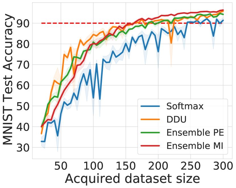
(a) MNIST

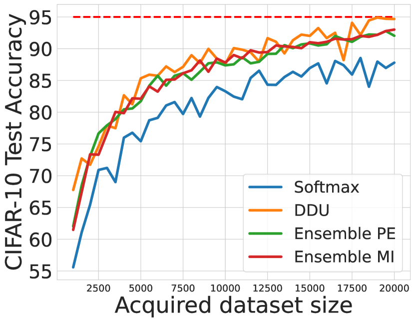
(b) CIFAR-10

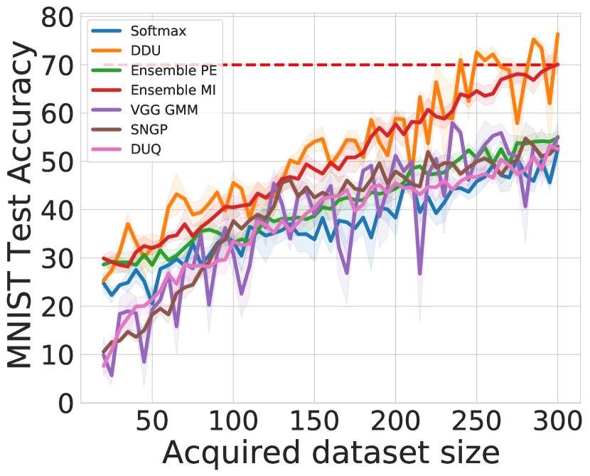
(c) Dirty-MNIST

Figure 5: Active Learning experiments. Acquired training set size vs test accuracy. DDU performs on par with Deep Ensembles.

4.1 Active Learning

We first demonstrate the quality of our uncertainty disentanglement in active learning (AL) (Cohn et al., 1996). AL aims to train models in a data-efficient manner. Additional training samples are iteratively acquired from a large pool of unlabelled data and labelled with the help of an expert. After each acquisition step, the model is retrained on the newly expanded training set. This is repeated until the model achieves a desirable accuracy—or when a maximum number of samples have been acquired.

Data-efficient acquisition relies on acquiring labels for the most informative samples. This can be achieved by selecting points with high epistemic uncertainty (Gal et al., 2017). Conversely, repeated acquisition of points with high aleatoric uncertainty is not informative for the model and such acquisitions lead to data inefficiency. AL, therefore, makes an excellent application for evaluating epistemic uncertainty and the ability of models to separate different sources of uncertainty. We evaluate DDU on three different setups: i) with clean MNIST samples in the pool set, ii) with clean CIFAR-10 samples in the pool set, and ii) with Dirty-MNIST, having a 1:60 ratio of MNIST to Ambiguous-MNIST samples, in the pool set. In the first two setups, we compare 3 baselines: i) a ResNet-18 with softmax entropy as the acquisition function, ii) DDU trained using a ResNet-18 with feature density as acquisition function, and iii) a Deep Ensemble of 3 ResNet-18s with the predictive entropy (PE) and mutual information (MI) of the ensemble as the acquisition functions. In the last setup, in addition to the above 3 approaches, we also use iv) feature density of a VGG-16 instead of ResNet-18+SN as an ablation to see if feature density of a model without inductive biases performs well, v) SNGP and vi) DUQ as additional baselines. For MNIST and Dirty-MNIST, we start with an initial training-set size of 20 randomly chosen MNIST points, and in each iteration, acquire the 5 samples with highest reported epistemic uncertainty. For each step, we train the models using Adam (Kingma & Ba, 2015) for 100 epochs and choose the one with the best validation set accuracy. We stop the process when the training set size reaches 300. For CIFAR-10, we start with 1000 samples and go up to 20000 samples with an acquisition size of 500 samples in each step.

MNIST & CIFAR-10 In Figure 55(a) and Figure 55(b), for regular curated MNIST and CIFAR-10 in the pool set, DDU clearly outperforms the deterministic softmax baseline and is competitive with Deep Ensembles. For MNIST, the softmax baseline reaches 90% test-set accuracy at a training-set size of 245. DDU reaches 90% accuracy at a training-set size of 160, whereas Deep Ensemble reaches the same at 185 and 155 training samples with PE and MI as the acquisition functions respectively. Note that DDU is three times faster than a Deep Ensemble, which needs to train three models independently after every acquisition.

Dirty-MNIST. Real-life datasets often contain observation noise and ambiguous samples. What happens when the pool set contains a lot of such noisy samples having high aleatoric uncertainty? In such cases, it becomes important for models to identify unseen and informative samples with high epistemic uncertainty and not with high aleatoric uncertainty. To study this, we construct a pool set with samples from Dirty-MNIST (see §B). We significantly increase the proportion of ambiguous samples by using a 1:60 split of MNIST to Ambiguous-MNIST (a total of 1K MNIST and 60K Ambiguous-MNIST samples). In Figure 55(c), for Dirty-MNIST in the pool set, the difference in the performance of DDU and the deterministic softmax model is stark. While DDU achieves a test set accuracy of 70% at a training set size of 240 samples, the accuracy of the softmax baseline peaks at a mere 50%. In addition, all baselines, including SNGP, DUQ and the feature density of a VGG-16, which fail to solely capture epistemic uncertainty, are significantly outperformed by DDU and the MI baseline of the deep ensemble. However, note that DDU also performs better than Deep Ensembles with the PE acquisition function. The difference gets larger as the training set size grows: DDU’s feature density and Deep Ensemble’s MI solely capture epistemic uncertainty and hence, do not get confounded by iD ambiguous samples with high aleatoric uncertainty.

4.2 OoD Detection

Table 2: OoD detection performance of different baselines using ResNet-50, Wide-ResNet-50-2 and VGG-16 architectures on ImageNet vs ImageNet-O (Hendrycks et al., 2021). Best AUROC scores are marked in bold.

Model	Accuracy ($\uparrow$)		ECE ($\downarrow$)		AUROC ($\uparrow$)
	Deterministic	3-Ensemble	Deterministic	3-Ensemble	Softmax Entropy	Energy-based Model	DDU	3-Ensemble PE	3-Ensemble MI
ResNet-50	$74.8\pm 0.05$	$76.01$	$2.08\pm 0.11$	$2.07$	$50.65\pm 0.63$	$53.88\pm 0.80$	$\mathbf{59.44\pm 0.15}$	$51.19$	$55.46$
Wide-ResNet-50-2	$76.75\pm 0.11$	$77.58$	$1.18\pm 0.07$	$1.22$	$50.44\pm 0.25$	$54.92\pm 0.43$	$\mathbf{63.15\pm 0.18}$	$51.83$	$57.98$
VGG-16	$72.48\pm 0.02$	$73.54$	$2.62\pm 0.11$	$2.59$	$50.51\pm 0.25$	$51.15\pm 0.27$	$51.73\pm 0.21$	$51.89$	$\mathbf{56.56}$

OoD detection is an application of epistemic uncertainty quantification: if we do not train on OoD data, we expect OoD data points to have higher epistemic uncertainty than iD data. We evaluate CIFAR-10 vs SVHN/CIFAR-100/Tiny-ImageNet/CIFAR-10-C, CIFAR-100 vs SVHN/Tiny-ImageNet and ImageNet vs ImageNet-O as iD vs OoD dataset pairs for this experiment (Krizhevsky et al., 2009; Netzer et al., 2011; Deng et al., 2009; Hendrycks & Dietterich, 2019). We also evaluate DDU on different architectures: Wide-ResNet-28-10, Wide-ResNet-50-2, ResNet-50, ResNet-110 and DenseNet-121 (Zagoruyko & Komodakis, 2016; He et al., 2016; Huang et al., 2017). The training setup is described in §D.2. In addition to using softmax entropy of a deterministic model (Softmax) for both aleatoric and epistemic uncertainty, we also compare with the following baselines that do not require training or fine-tuning on OoD data:

• Energy-based model (Liu et al., 2020b): We use the softmax entropy of a deterministic model as aleatoric uncertainty and the unnormalized softmax density (the logsumexp of the logits) as epistemic uncertainty without regularisation to avoid feature collapse. We only compare with the version that does not train on OoD data.

• DUQ (van Amersfoort et al., 2020) & SNGP (Liu et al., 2020a): We compare with the state-of-the-art deterministic methods for uncertainty quantification including DUQ and SNGP. For SNGP, we use the exact predictive covariance computation and we use the entropy of the average of the MC softmax samples as uncertainty. For DUQ, we use the closest kernel distance. Note that for CIFAR-100, DUQ’s one-vs-all objective did not converge during training and hence, we do not include the DUQ baseline for CIFAR-100.

• 5-Ensemble: We use an ensemble of 5 networks and compute the predictive entropy of the ensemble as both epistemic and aleatoric uncertainty and mutual information as epistemic uncertainty.

Table 1 shows the AUROC scores for Wide-ResNet-28-10 based models on CIFAR-10 vs SVHN/CIFAR-100/Tiny-ImageNet and CIFAR-100 vs SVHN/Tiny-ImageNet along with their respective test set accuracy and test set ECE after temperature scaling. The equivalent results for the other architectures, ResNet-50, ResNet-110 and DenseNet-121 can be found in Table 4, Table 5 and Table 6 respectively in the appendix. Note that for DDU, post-hoc calibration, e.g. in the form of temperature scaling (Guo et al., 2017), is straightforward as it does not affect the GMM density. In addition, we plot the AUROC averaged over all corruption types vs corruption intensity for CIFAR-10 vs CIFAR-10-C in Figure 1, with detailed AUROC plots for each corruption type in Figure 8, Figure 9, Figure 10 and Figure 11 of the appendix. Finally, in Table 2, we present AUROC scores for models trained on ImageNet.

For OoD detection, DDU outperforms all other deterministic single-forward-pass methods, DUQ, SNGP and the energy-based model approach from Liu et al. (2020b), on CIFAR-10 vs SVHN/CIFAR-100/Tiny-ImageNet, CIFAR-10 vs CIFAR-10-C and CIFAR-100 vs SVHN/Tiny-ImageNet, often performs on par with state-of-the-art Deep Ensembles—and even performing better in a few cases. This holds true for all the architectures we experimented on. Similar observations can be made on ImageNet vs ImageNet-O as well. Importantly, the great performance in OoD detection comes without compromising on the single-model test set accuracy in comparison to other deterministic methods.

Additional ablations for the CIFAR-10/100 experiments are detailed in §E: Table 7 and 8. These tables along with observations in Table 2, show that the feature density of a VGG-16 (i.e. without residual connections and spectral normalisation) is unable to beat a VGG-16 ensemble, whereas a Wide-ResNet-28-10 with spectral normalisation outperforms its corresponding ensemble in almost all the cases. This result further validates the importance of having the bi-Lipschitz constraint (spectral normalisation) on the model to obtain smoothness and sensitivity. Finally, even without spectral normalisation, a Wide-ResNet-28 has the inductive bias of residual connections built into its model architecture, which can be a contributing factor towards good performance in general as residual connections already make the model sensitive to changes in the input space.

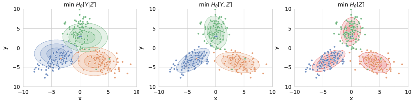
(a) Density. Contours at 68.26%, 95.44%, and 99.7%.

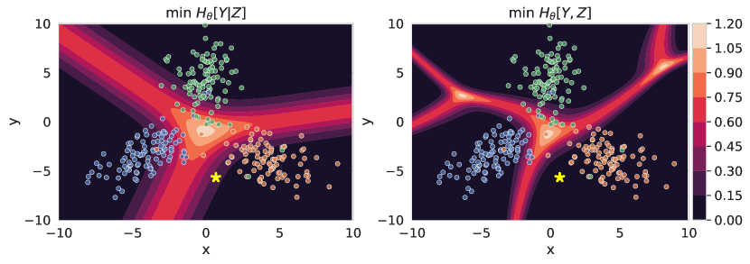
(b) Entropy. Darker is lower.

Figure 6: 3-component GMM fitted to a synthetic dataset with 3 different classes (differently colored) with 4% label noise using different objectives. 6(a): The optimas for conditional log-likelihood $\operatorname{\mathbb{H}_{\theta}}[Y\mathbin{|}Z]$, joint log-likelihood $\operatorname{\mathbb{H}_{\theta}}[Y,Z]$, and marginalised log-likehood $\operatorname{\mathbb{H}_{\theta}}[Z]$ all differ. Hence, the best calibrated model ($\operatorname{\mathbb{H}_{\theta}}[Y\mathbin{|}Z]$) will not provide the best density estimate ($\operatorname{\mathbb{H}_{\theta}}[Z]$), and vice-versa. 6(b): A mixture model that optimizes $\operatorname{\mathbb{H}_{\theta}}[Y,Z]$ (GDA) does not have calibrated decision boundaries for aleatoric uncertainty: the ambiguous sample (due to label noise) marked by the yellow star has no aleatoric uncertainty under the GDA model. See §G.2.3 for details.

5 Additional Insights

We elaborate on potential pitfalls of predictive entropy in general and softmax entropy of determinstic models in particular in the following section. Additional proofs for all statements in this section are provided in §G.

Potential Pitfalls of Predictive Entropy. Conceptually, we note that predictive entropy confounds epistemic and aleatoric uncertainty. Ensembling might also be seen as performing Bayesian Model Averaging (He et al., 2020; Wilson & Izmailov, 2020), as each ensemble member, producing a softmax output $\operatorname{p}(y\mathbin{|}x,\omega)$, can be considered to be drawn from some distribution $\operatorname{p}(\omega\mathbin{|}\mathcal{D})$ over the trained model parameters $\omega$, which is induced by the pushforward of the weight initialization under stochastic optimization. As a result, eq. (1) can also be applied to Deep Ensembles to disentangle epistemic from predictive uncertainty via computing the mutual information. Both mutual information $\operatorname{\mathbb{I}}[Y;\omega\mathbin{|}x,\mathcal{D}]$ and predictive entropy $\operatorname{\mathbb{H}}[Y\mathbin{|}x,\mathcal{D}]$ could be used to detect OoD samples. However, previous empirical findings show the predictive entropy outperforming mutual information (Malinin & Gales, 2018). Indeed, much of recent literature only focuses on predictive entropy and the related confidence score for OoD detection (see §A.1 for a review). This can be explained by the following observation:

Observation 5.1.

When we already know that aleatoric uncertainty or epistemic uncertainty is low for a sample, predictive entropy is a good measure of the other quantity.

Hence, the predictive entropy as an upper-bound of the mutual information can separate iD and OoD data better for curated datasets with low aleatoric uncertainty. However, as seen in eq. (1), predictive entropy can be high for both iD ambiguous samples (high aleatoric uncertainty) as well as for OoD samples (high epistemic uncertainty) (see Figure 4) and might not be an effective measure for OoD detection when used with datasets that are not curated and ambiguous samples, like Dirty-MNIST in Figure 2.

Potential Pitfalls of Softmax Entropy. The softmax entropy for deterministic models trained with maximum likelihood can be inconsistent. The mechanism underlying Deep Ensemble uncertainty that pushes epistemic uncertainty to be high on OoD data is the function disagreement between different ensemble components, i.e. arbitrary predictive extrapolations of the softmax models composing the ensemble:

Proposition 5.2.

Let $x_{1}$ and $x_{2}$ be points such that $x_{1}$ has higher epistemic uncertainty than $x_{2}$ under the ensemble: $\operatorname{\mathbb{I}}[Y_{1};\omega\mathbin{|}x_{1},\mathcal{D}]>\operatorname{\mathbb{I}}[Y_{2};\omega\mathbin{|}x_{2},\mathcal{D}]+\delta,$ $\delta\geq 0$. Further assume both have similar predictive entropy $|\operatorname{\mathbb{H}}[Y_{1}\mathbin{|}x_{1},\mathcal{D}]-\operatorname{\mathbb{H}}[Y_{2}\mathbin{|}x_{2},\mathcal{D}]|\leq\epsilon,$ $\epsilon\geq 0$. Then, there exist sets of ensemble members $\Omega$ with $\operatorname{p}(\Omega\mathbin{|}\mathcal{D})>0$, such that for all softmax models $\omega\in\Omega$ the softmax entropy of $x_{1}$ is lower than the softmax entropy of $x_{2}$: $\operatorname{\mathbb{H}}[Y_{1}\mathbin{|}x_{1},\omega]<\operatorname{\mathbb{H}}[Y_{2}\mathbin{|}x_{2},\omega]-(\delta-\epsilon)$.

If a sample is assigned higher epistemic uncertainty (in the form of mutual information) by a Deep Ensemble than another sample, it will necessarily be assigned lower softmax entropy by at least one of the ensemble’s members. As a result, a priori, we cannot know whether a softmax model preserves the order or not, and the empirical observation that the mutual information of an ensemble can quantify epistemic uncertainty well implies that the softmax entropy of a deterministic model might not. This can be seen in Figure 2(b), 4 and §G.1.3 where we observe the softmax entropy for OoD samples to have values which can be high, low or anywhere in between. Note not all model architectures will behave like this, but when the mutual information of a corresponding Deep Ensemble works well empirically (for example in active learning), Proposition 5.2 holds.

Objective Mismatch. The predictive probability induced by a feature-density estimator will generally not be well-calibrated as there is an objective mismatch. This was overlooked in previous research on uncertainty quantification for deterministic models (Lee et al., 2018b; Liu et al., 2020a; van Amersfoort et al., 2020; He et al., 2016; Postels et al., 2020). Specifically, a mixture model $\operatorname{q}(y,z)=\sum_{y}\operatorname{q}(z\mathbin{|}y)\operatorname{q}(y)$, using one component per class, cannot be optimal for both feature-space density and predictive distribution estimation as there is an objective mismatch:

Proposition 5.3.

For an input $x$, let $z=f_{\theta}(x)$ denote its feature representation in a feature extractor $f_{\theta}$ with parameters $\theta$. Then the following hold:

1. A discriminative classifier $\operatorname{p}(y\mathbin{|}z)$, e.g. a softmax layer, is well-calibrated in its predictions when it maximises the conditional log-likelihood $\log\operatorname{p}(y\mathbin{|}z)$;

2. A feature-space density estimator $\operatorname{q}(z)$ is optimal when it maximises the marginalised log-likelihood $\log\operatorname{q}(z)$;

3. A mixture model $\operatorname{q}(y,z)=\sum_{y}\operatorname{q}(z\mathbin{|}y)\operatorname{q}(y)$ might not maximise both objectives, conditional log-likelihood and marginalised log-likelihood, at the same time. In the specific instance that a GMM with one component per class does maximise both, the resulting model must be a GDA (but the opposite does not hold).

Hence, importantly, DDU uses both a discriminative classifier (softmax layer) to capture aleatoric uncertainty for iD samples and a separate feature-density estimator to capture epistemic uncertainty even on a model trained using conditional log-likelihood, i.e. the usual cross-entropy objective. Figure 6 and §G.2.3 provide additional intuitions.

6 Conclusion

Deep Deterministic Uncertainty (DDU) can outperform state-of-the-art deterministic single-pass uncertainty methods in active learning and OoD detection by fitting a GDA for feature-space density estimation after training a model with residual connections and spectral normalization (Lee et al., 2018b; Liu et al., 2020a), and it manages to perform as well as deep ensembles in various settings. Hence, DDU provides a very simple method to produce good epistemic and aleatoric uncertainty estimates and might be taken into consideration as an alternative to deep ensembles without requiring the complexities or computational cost of the current state-of-the-art. Reliable uncertainty quantification is an important requirement to make deep neural nets safe for deployment. Thus, we hope our work will contribute to increasing safety, reliability and trust in AI.

Appendix A Related Work

Several existing approaches model uncertainty using feature-space density but underperform without fine-tuning on OoD data. Our work identifies feature collapse and objective mismatch as possible reasons for this. Among these approaches, Lee et al. (2018b) uses Mahalanobis distances to quantify uncertainty by fitting a class-wise Gaussian distribution (with shared covariance matrices) on the feature space of a pre-trained ResNet encoder. The competitive results they report require input perturbations, ensembling GMM densities from multiple layers, and fine-tuning on OoD hold-out data. They do not discuss any constraints which the ResNet encoder should satisfy, and therefore, are vulnerable to feature collapse. In Figure 2(c), for example, the feature density of a LeNet and a VGG are unable to distinguish OoD from iD samples. Postels et al. (2020) also propose a density-based estimation of aleatoric and epistemic uncertainty. Similar to Lee et al. (2018b), they do not constrain their pre-trained ResNet encoder. They do discuss feature collapse though, noting that they do not address this problem. Moreover, they do not consider the objective mismatch that arises (see Proposition 5.3 below) and use a single estimator for both epistemic and aleatoric uncertainty. Consequently, they report worse epistemic uncertainty: 74% AUROC on CIFAR-10 vs SVHN, which we show to considerably fall behind modern approaches for uncertainty estimation in deep learning in §4. Likewise, Liu et al. (2020b) compute an unnormalized density based on the softmax logits without taking into account the need for inductive biases to ensure smoothness and sensitivity of the feature space.

Winkens et al. (2020) use contrastive training on the feature extractor before estimating the feature-space density. Our method is orthogonal from this work as we restrict ourselves to the supervised setting and show that the inductive biases that result in bi-Lipschitzness (van Amersfoort et al., 2020; Liu et al., 2020a) are sufficient for the feature-space density to reliably capture epistemic uncertainty.

Lastly, our method improves upon van Amersfoort et al. (2020) and Liu et al. (2020a) by alleviating the need for additional hyperparameters: DDU only needs minimal changes from the standard softmax setup to outperform DUQ and SNGP on uncertainty benchmarks, and our GMM parameters are optimised for the already trained model using the training set. In particular, DDU does not require training or fine-tuning with OoD data. Moreover, our insights in §5 explain why Liu et al. (2020a) found that a baseline that uses the softmax entropy instead of the feature-space density of a deterministic network with bi-Lipschitz constraint underperforms.

A.1 Predictive Entropy and Confidence in Recent Works

Table 3 shows a selection of recently published papers which use entropy or confidence as OoD score. Only two papers examine using Mutual Information with Deep Ensembles as OoD score at all. None of the papers examines the possible confounding of aleatoric and epistemic uncertainty when using predictive entropy or confidence, or the consistency issues of softmax entropy (and softmax confidence), detailed in §5. This list is not exhaustive, of course.

Table 3: A sample of recently published papers and OoD metrics. Many recently published papers only use Predictive Entropy or Predictive Confidence (for Deep Ensembles) or Softmax Confidence (for deterministic models) as OoD scores without addressing the possible confounding of aleatoric and epistemic uncertainty, that is ambiguous iD samples with OoD samples. Only two papers examine using Mutual Information with Deep Ensembles as OoD score at all.

Title	Citation	Softmax Confidence	Predictive Confidence	Predictive Entropy	Mutual Information
A Baseline for Detecting Misclassified and Out-of-Distribution Examples in Neural Networks	Hendrycks & Gimpel (2016)	✓	✗	✗	✗
Deep Anomaly Detection with Outlier Exposure	Hendrycks et al. (2018)	✓	✗	✗	✗
Enhancing The Reliability of Out-of-distribution Image Detection in Neural Networks	Liang et al. (2018)	✓	✗	✗	✗
Training Confidence-calibrated Classifiers for Detecting Out-of-Distribution Samples	Lee et al. (2018a)	✓	✗	✗	✗
Learning Confidence for Out-of-Distribution Detection in Neural Networks	DeVries & Taylor (2018)	✓	✗	✗	✗
Simple and Scalable Predictive Uncertainty Estimation using Deep Ensembles	Lakshminarayanan et al. (2017)	✗	✓	✓	✗
Predictive Uncertainty Estimation via Prior Networks	Malinin & Gales (2018)	✗	✓	✓	✓
Ensemble Distribution Distillation	Malinin et al. (2020)	✗	✗	✓	✓
Generalized ODIN: Detecting Out-of-Distribution Image Without Learning From Out-of-Distribution Data	Hsu et al. (2020)	✓	✗	✗	✗
Being Bayesian, Even Just a Bit, Fixes Overconfidence in ReLU Networks	Kristiadi et al. (2020)	✗	✓	✗	✗

Appendix B Ambiguous- and Dirty-MNIST

Each sample in Ambiguous-MNIST is constructed by decoding a linear combination of latent representations of 2 different MNIST digits from a pre-trained VAE (Kingma & Welling, 2014). Every decoded image is assigned several labels sampled from the softmax probabilities of an off-the-shelf MNIST neural network ensemble, with points filtered based on an ensemble’s MI (to remove ‘junk’ images) and then stratified class-wise based on their softmax entropy (some classes are inherently more ambiguous, so we “amplify” these; we stratify per-class to try to preserve a wide spread of possible entropy values, and avoid introducing additional ambiguity which will increase all points to have highest entropy). All off-the-shelf MNIST neural networks were then discarded and new models were trained to generate Fig 1 (and as can be seen, the ambiguous points we generate indeed have high entropy regardless of the model architecture used). We create 60K such training and 10K test images to construct Ambiguous-MNIST. Finally, the Dirty-MNIST dataset in this experiment contains MNIST and Ambiguous-MNIST samples in a 1:1 ratio (with 120K training and 20K test samples). In Figure 7, we provide some samples from Ambiguous-MNIST.

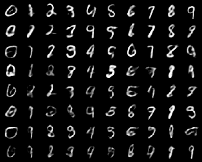
Figure 7: Samples from Ambiguous-MNIST.

Appendix C Algorithm

Algorithm 1 Deep Deterministic Uncertainty

Definitions:- Regularized feature extractor $f_{\theta}:x\rightarrow\mathbb{R}^{d}$- Softmax output predictions: $p(y|x)$- GMM density: $q(z)=\sum_{y}q(z|y=c)\,q(y=c)$- Dataset $(X,Y)$

0:   train train NN $p(y|f_{\theta}(x))$ with $(X,Y)$ each class $c$ with samples $\mathbf{x}_{c}\subset X$ $\mu_{c}\leftarrow\frac{1}{|\mathbf{x}_{c}|}\sum_{\mathbf{x}_{c}}f_{\theta}(\mathbf{x}_{c})$ $\Sigma_{c}\leftarrow\frac{1}{|\mathbf{x}_{c}|-1}(f_{\theta}(\mathbf{x}_{c})-\mu_{c})(f_{\theta}(\mathbf{x}_{c})-\mu_{c})^{T}$ $\pi_{c}\leftarrow\frac{\sum_{\mathbf{x}_{c}}1}{\lvert X\rvert}$

0:   disentangle_uncertaintysample $x$ compute feature representation $z=f_{\theta}(x)$ compute density under GMM: $q(z)=\sum_{y}\operatorname{q}(z\mathbin{|}y)\operatorname{q}(y)$ with $\operatorname{q}(z\mathbin{|}y)\sim\mathcal{N}(\mu_{y};\sigma_{y}),\operatorname{q}(y)=\pi_{y}$ compute softmax entropy: $H_{p}[Y|x]$

0:   low density $q(z)$ OoD high density $q(z)$ high entropy $H_{p}[Y|x]$ ambiguous iD low entropy $H_{p}[Y|x]$ iD

⬇

# instantiate models

model = create_sensitive_smooth_model()

gda = create_gda()

# train

training_samples, training_labels = load_training_set()

model.fit(training_samples, training_labels)

training_features = model.features(training_samples)

gda.fit(training_features, training_labels)

# test

test_features = model.features(test_sample)

epistemic_uncertainty = gda.log_density(test_features)

is_ood = ood_threshold <= epistemic_uncertainty

if not is_ood:

predictions = model.softmax_layer(test_features)

aleatoric_uncertainty = entropy(predictions)

Listing 1: Deep Deterministic Uncertainty Pseudo-Code

C.1 Increasing sensitivity

Using residual connections to enforce sensitivity works well in practice when the layer is defined as $x^{\prime}=x+f(x)$. However, there are several places in the network where additional spatial downsampling is done in $f(\cdot)$ (through a strided convolution), and in order to compute the residual operation $x$ needs to be downsampled as well. These downsampling operations are crucial for managing memory consumption and generalisation. The way this is traditionally done in ResNets is by introducing an additional function $g(\cdot)$ on the residual branch (obtaining $x^{\prime}=g(x)+f(x)$) which is a strided 1x1 convolution. In practice, the stride is set to 2 pixels, which leads to the output of $g(\cdot)$ only being dependent on the top-left pixel of each 2x2 patch, which reduces sensitivity. We overcome this issue by making an architectural change that improves uncertainty quality without sacrificing accuracy. We use a strided average pooling operation instead of a 1x1 convolution in $g(\cdot)$. This makes the output of $g(\cdot)$ dependent on all input pixels. Additionally, we use leaky ReLU activation functions, which are equivalent to ReLU activations when the input is larger than 0, but below 0 they compute $p*x$ with $p=0.01$ in practice. These further improve sensitivity as all negative activations still propagate in the network.

C.2 Algorithm & Pseudo-Code Implementation

The algorithm is provided in Algorithm 1. A simple Python pseudo-code implementation using a scikit-learn-like API (Buitinck et al., 2013) is shown in LABEL:algorithm. Note that in order to compute thresholds for low and high density or entropy, we can simply use the training set containing iD data. We set all points having density lower than $99\%$ quantile as OoD.

Appendix D Experimental Details

D.1 Dirty-MNIST

We train for 50 epochs using SGD with a momentum of 0.9 and an initial learning rate of 0.1. The learning rate drops by a factor of 10 at training epochs 25 and 40. Following SNGP (Liu et al., 2020a), we apply online spectral normalisation with one step of a power iteration on the convolutional weights. For 1x1 convolutions, we use the exact algorithm, and for 3x3 convolutions, the approximate algorithm from Gouk et al. (2021). The coefficient for SN is a hyper-parameter which we set to 3 using cross-validation.

D.2 OoD Detection Training Setup

We train the softmax baselines on CIFAR-10/100 for 350 epochs using SGD as the optimiser with a momentum of 0.9, and an initial learning rate of 0.1. The learning rate drops by a factor of 10 at epochs 150 and 250. We train the 5-Ensemble baseline using this same training setup. The SNGP and DUQ models were trained using the setup of SNGP and hyper-parameters mentioned in their respective papers (Liu et al., 2020a; van Amersfoort et al., 2020). For models trained on ImageNet, we train for 90 epochs with SGD optimizer, an initial learning rate of 0.1 and a weight decay of 1e-4. We use a learning rate warmup decay of 0.01 along with a step scheduler with step size of 30 and a step factor of 0.1.

D.3 Compute Resources

Each model (ResNet-18, Wide-ResNet-28-10, ResNet-50, ResNet-110, DenseNet-121 or VGG-16) used for the large scale active learning, CIFAR-10 vs SVHN/CIFAR-100/Tiny-ImageNet/CIFAR-10-C and CIFAR-100 vs SVHN/Tiny-ImageNet tasks was trained on a single Nvidia Quadro RTX 6000 GPU. Each model (LeNet, VGG-16 and ResNet-18) used to get the results in Figure 2 and Table 9 was trained on a single Nvidia GeForce RTX 2060 GPU. Each model (ResNet-50, Wide-ResNet-50-2, VGG-16) trained on ImageNet was trained using 8 Nvidia Quadro RTX 6000 GPUs.

Table 4: OoD detection performance of different baselines using a ResNet-50 architecture with the CIFAR-10 vs SVHN/CIFAR-100/Tiny-ImageNet and CIFAR-100 vs SVHN/Tiny-ImageNet dataset pairs averaged over 25 runs. Note: SN stands for Spectral Normalisation, JP stands for Jacobian Penalty. We highlight the best deterministic and best method overall in bold for each metric.

Train Dataset	Method	Penalty	Aleatoric Uncertainty	Epistemic Uncertainty	Test Accuracy ($\uparrow$)	Test ECE ($\downarrow$)	AUROC SVHN ($\uparrow$)	AUROC CIFAR-100 ($\uparrow$)	AUROC Tiny-ImageNet ($\uparrow$)
CIFAR-10	Softmax	-	Softmax Entropy	Softmax Entropy	$\mathbf{95.04\pm 0.05}$	$\mathbf{0.97\pm 0.04}$	$93.80\pm 0.41$	$88.91\pm 0.07$	$88.32\pm 0.07$
	Energy-based (Liu et al., 2020b)	-		Softmax Density			$94.48\pm 0.44$	$88.84\pm 0.08$	$88.45\pm 0.08$
	DUQ (van Amersfoort et al., 2020)	JP	Kernel Distance	Kernel Distance	$94.05\pm 0.11$	$1.71\pm 0.07$	$93.14\pm 0.43$	$83.87\pm 0.27$	$84.28\pm 0.26$
	SNGP (Liu et al., 2020a)	SN	Predictive Entropy	Predictive Entropy	$94.90\pm 0.11$	$1.01\pm 0.03$	$93.15\pm 0.85$	$89.32\pm 0.10$	$88.96\pm 0.13$
	DDU (ours)	SN	Softmax Entropy	GMM Density	$94.92\pm 0.06$	$1\pm 0.04$	$\mathbf{94.77\pm 0.35}$	$\mathbf{89.98\pm 0.17}$	$\mathbf{89.12\pm 0.13}$
	5-Ensemble	-	Predictive Entropy	Predictive Entropy	$\mathbf{96.06\pm 0.04}$	$1.65\pm 0.07$	$94.75\pm 0.39$	$89.87\pm 0.06$	$88.69\pm 0.05$
	(Lakshminarayanan et al., 2017)			Mutual Information			$94.09\pm 0.20$	$89.76\pm 0.06$	$89.04\pm 0.03$
					Test Accuracy ($\uparrow$)	Test ECE ($\downarrow$)	AUROC SVHN ($\uparrow$)		AUROC Tiny-ImageNet ($\uparrow$)
CIFAR-100	Softmax	-	Softmax Entropy	Softmax Entropy	$77.91\pm 0.09$	$4.32\pm 0.10$	$81.32\pm 0.65$		$79.83\pm 0.07$
	Energy-based (Liu et al., 2020b)	-		Softmax Density			$82.05\pm 0.69$		$79.61\pm 0.08$
	SNGP (Liu et al., 2020a)	SN	Predictive Entropy	Predictive Entropy	$74.73\pm 0.22$	$7.68\pm 0.13$	$82.50\pm 2.09$		$77.05\pm 0.16$
	DDU (ours)	SN	Softmax Entropy	GMM Density	$\mathbf{79.26\pm 0.16}$	$\mathbf{4.07\pm 0.06}$	$\mathbf{87.34\pm 0.64}$		$\mathbf{82.11\pm 0.20}$
	5-Ensemble	-	Predictive Entropy	Predictive Entropy	$\mathbf{81.06\pm 0.07}$	$\mathbf{3.54\pm 0.12}$	$83.42\pm 0.89$		$77.69\pm 0.12$
	(Lakshminarayanan et al., 2017)			Mutual Information			$84.24\pm 0.90$		$81.59\pm 0.05$

Table 5: OoD detection performance of different baselines using a ResNet-110 architecture with the CIFAR-10 vs SVHN/CIFAR-100/Tiny-ImageNet and CIFAR-100 vs SVHN/Tiny-ImageNet dataset pairs averaged over 25 runs. Note: SN stands for Spectral Normalisation, JP stands for Jacobian Penalty. We highlight the best deterministic and best method overall in bold for each metric.

Train Dataset	Method	Penalty	Aleatoric Uncertainty	Epistemic Uncertainty	Test Accuracy ($\uparrow$)	Test ECE ($\downarrow$)	AUROC SVHN ($\uparrow$)	AUROC CIFAR-100 ($\uparrow$)	AUROC Tiny-ImageNet ($\uparrow$)
CIFAR-10	Softmax	-	Softmax Entropy	Softmax Entropy	$\mathbf{95.08\pm 0.04}$	$1.02\pm 0.04$	$93.12\pm 0.44$	$88.7\pm 0.1$	$88.07\pm 0.11$
	Energy-based (Liu et al., 2020b)	-		Softmax Density			$93.67\pm 0.47$	$88.60\pm 0.11$	$88.13\pm 0.11$
	DUQ (van Amersfoort et al., 2020)	JP	Kernel Distance	Kernel Distance	$94.32\pm 0.17$	$1.21\pm 0.07$	$94.02\pm 0.45$	$86.17\pm 0.35$	$85.24\pm 0.21$
	SNGP (Liu et al., 2020a)	SN	Predictive Entropy	Predictive Entropy	$94.85\pm 0.09$	$1.04\pm 0.02$	$93.17\pm 0.53$	$89.23\pm 0.10$	$88.80\pm 0.12$
	DDU (ours)	SN	Softmax Entropy	GMM Density	$94.82\pm 0.06$	$\mathbf{1.01\pm 0.04}$	$\mathbf{95.48\pm 0.30}$	$\mathbf{90.08\pm 0.13}$	$\mathbf{89.18\pm 0.15}$
	5-Ensemble	-	Predictive Entropy	Predictive Entropy	$\mathbf{96.18\pm 0.05}$	$1.57\pm 0.05$	$95.07\pm 0.45$	$\mathbf{90.23\pm 0.04}$	$89\pm 0.03$
	(Lakshminarayanan et al., 2017)			Mutual Information			$94.72\pm 0.34$	$89.69\pm 0.05$	$88.35\pm 0.05$
					Test Accuracy ($\uparrow$)	Test ECE ($\downarrow$)	AUROC SVHN ($\uparrow$)		AUROC Tiny-ImageNet ($\uparrow$)
CIFAR-100	Softmax	-	Softmax Entropy	Softmax Entropy	$78.65\pm 0.10$	$3.93\pm 0.13$	$82.04\pm 0.57$		$80.13\pm 0.07$
	Energy-based (Liu et al., 2020b)	-		Softmax Density			$82.78\pm 0.60$		$80.01\pm 0.09$
	SNGP (Liu et al., 2020a)	SN	Predictive Entropy	Predictive Entropy	$76.16\pm 0.27$	$6.43\pm 0.75$	$83.94\pm 0.10$		$78.54\pm 0.28$
	DDU (ours)	SN	Softmax Entropy	GMM Density	$\mathbf{78.89\pm 0.17}$	$\mathbf{3.79\pm 0.07}$	$\mathbf{88.66\pm 0.56}$		$\mathbf{82.58\pm 0.24}$
	5-Ensemble	-	Predictive Entropy	Predictive Entropy	$\mathbf{81.80\pm 0.10}$	$\mathbf{3.67\pm 0.11}$	$83.68\pm 0.33$		$81.12\pm 0.13$
	(Lakshminarayanan et al., 2017)			Mutual Information			$85.11\pm 0.57$		$81.94\pm 0.06$

Table 6: OoD detection performance of different baselines using a DenseNet-121 architecture with the CIFAR-10 vs SVHN/CIFAR-100/Tiny-ImageNet and CIFAR-100 vs SVHN/Tiny-ImageNet dataset pairs averaged over 25 runs. Note: SN stands for Spectral Normalisation, JP stands for Jacobian Penalty. We highlight the best deterministic and best method overall in bold for each metric.

Train Dataset	Method	Penalty	Aleatoric Uncertainty	Epistemic Uncertainty	Test Accuracy ($\uparrow$)	Test ECE ($\downarrow$)	AUROC SVHN ($\uparrow$)	AUROC CIFAR-100 ($\uparrow$)	AUROC Tiny-ImageNet ($\uparrow$)
CIFAR-10	Softmax	-	Softmax Entropy	Softmax Entropy	$95.16\pm 0.03$	$1.10\pm 0.04$	$94\pm 0.44$	$87.55\pm 0.11$	$86.99\pm 0.12$
	Energy-based (Liu et al., 2020b)	-		Softmax Density			$94.07\pm 0.54$	$86.73\pm 0.15$	$86.43\pm 0.16$
	DUQ (van Amersfoort et al., 2020)	JP	Kernel Distance	Kernel Distance	$95.02\pm 0.14$	$1.08\pm 0.08$	$94.67\pm 0.41$	$87.38\pm 0.21$	$86.72\pm 0.14$
	SNGP (Liu et al., 2020a)	SN	Predictive Entropy	Predictive Entropy	$94.31\pm 0.21$	$1.08\pm 0.10$	$94.48\pm 0.34$	$88.86\pm 0.46$	$88.40\pm 0.48$
	DDU (ours)	SN	Softmax Entropy	GMM Density	$\mathbf{95.21\pm 0.03}$	$\mathbf{1.05\pm 0.03}$	$\mathbf{96.21\pm 0.31}$	$\mathbf{90.84\pm 0.06}$	$\mathbf{89.70\pm 0.06}$
	5-Ensemble	-	Predictive Entropy	Predictive Entropy	$\mathbf{96.18\pm 0.05}$	$1.07\pm 0.07$	$95.78\pm 0.11$	$90.65\pm 0.03$	$89.62\pm 0.06$
	(Lakshminarayanan et al., 2017)			Mutual Information			$95.75\pm 0.10$	$90.71\pm 0.04$	$89.34\pm 0.06$
					Test Accuracy ($\uparrow$)	Test ECE ($\downarrow$)	AUROC SVHN ($\uparrow$)		AUROC Tiny-ImageNet ($\uparrow$)
CIFAR-100	Softmax	-	Softmax Entropy	Softmax Entropy	$79.02\pm 0.08$	$4.11\pm 0.08$	$85.86\pm 0.42$		$81.10\pm 0.07$
	Energy-based (Liu et al., 2020b)	-		Softmax Density			$87.09\pm 0.49$		$80.84\pm 0.08$
	SNGP (Liu et al., 2020a)	SN	Predictive Entropy	Predictive Entropy	$79.15\pm 0.15$	$6.73\pm 0.10$	$85.00\pm 0.12$		$79.76\pm 0.15$
	DDU (ours)	SN	Softmax Entropy	GMM Density	$\mathbf{79.15\pm 0.07}$	$\mathbf{4.11\pm 0.06}$	$\mathbf{88.44\pm 0.55}$		$\mathbf{81.85\pm 0.11}$
	5-Ensemble	-	Predictive Entropy	Predictive Entropy	$\mathbf{81.01\pm 0.13}$	$4.81\pm 0.05$	$88.32\pm 0.61$		$81.45\pm 0.12$
	(Lakshminarayanan et al., 2017)			Mutual Information			$88.36\pm 0.17$		$81.73\pm 0.06$

Table 7: OoD detection performance of different ablations trained on CIFAR-10 using Wide-ResNet-28-10 and VGG-16 architectures with SVHN, CIFAR-100 and Tiny-ImageNet as OoD datasets averaged over 25 runs. Note: SN stands for Spectral Normalisation. We highlight the best deterministic and best method overall in bold for each metric.

Ablations					Aleatoric Uncertainty	Epistemic Uncertainty	Test Accuracy ($\uparrow$)	Test ECE ($\downarrow$)	AUROC SVHN ($\uparrow$)	AUROC CIFAR-100 ($\uparrow$)	AUROC Tiny-ImageNet ($\uparrow$)
Architecture	Ensemble	Residual Connections	SN	GMM
Wide-ResNet-28-10	✗	✓	✗	✗	Softmax Entropy	Softmax Entropy	$\mathbf{95.98\pm 0.02}$	$0.85\pm 0.02$	$94.44\pm 0.43$	$89.39\pm 0.06$	$88.42\pm 0.05$
						Softmax Density			$94.56\pm 0.51$	$88.89\pm 0.07$	$88.11\pm 0.06$
				✓	Softmax Entropy	GMM Density	$95.98\pm 0.02$	$0.85\pm 0.02$	$96.08\pm 0.25$	$90.94\pm 0.03$	$90.62\pm 0.05$
			✓	✗	Softmax Entropy	Softmax Entropy	$95.97\pm 0.03$	$0.85\pm 0.04$	$94.05\pm 0.26$	$90.02\pm 0.07$	$89.07\pm 0.06$
						Softmax Density			$94.31\pm 0.33$	$89.78\pm 0.08$	$88.96\pm 0.07$
				✓	Softmax Entropy	GMM Density	$95.97\pm 0.03$	$\mathbf{0.85\pm 0.04}$	$\mathbf{97.86\pm 0.19}$	$\mathbf{91.34\pm 0.04}$	$\mathbf{91.07\pm 0.05}$
	✓	✓	✗	✗	Predictive Entropy	Predictive Entropy	$\mathbf{96.59\pm 0.02}$	$\mathbf{0.76\pm 0.03}$	$97.73\pm 0.31$	$\mathbf{92.13\pm 0.02}$	$90.06\pm 0.03$
						Mutual Information			$97.18\pm 0.19$	$91.33\pm 0.03$	$90.90\pm 0.03$
VGG-16	✗	✓	✗	✗	Softmax Entropy	Softmax Entropy	$93.63\pm 0.04$	$1.64\pm 0.03$	$85.76\pm 0.84$	$82.48\pm 0.14$	$83.07\pm 0.12$
						Softmax Density			$84.24\pm 1.04$	$81.91\pm 0.17$	$82.82\pm 0.14$
				✓	Softmax Entropy	GMM Density	$93.63\pm 0.04$	$1.64\pm 0.03$	$89.25\pm 0.36$	$86.55\pm 0.10$	$86.78\pm 0.09$
			✓	✗	Softmax Entropy	Softmax Entropy	$93.62\pm 0.04$	$1.78\pm 0.04$	$87.54\pm 0.41$	$82.71\pm 0.09$	$83.33\pm 0.08$
						Softmax Density			$86.28\pm 0.51$	$82.15\pm 0.11$	$83.07\pm 0.10$
				✓	Softmax Entropy	GMM Density	$93.62\pm 0.04$	$1.78\pm 0.04$	$89.62\pm 0.37$	$86.37\pm 0.14$	$86.63\pm 0.11$
	✓	✓	✗	✗	Predictive Entropy	Predictive Entropy	$94.9\pm 0.05$	$2.03\pm 0.03$	$92.80\pm 0.18$	$89.01\pm 0.08$	$87.66\pm 0.08$
						Mutual Information			$91\pm 0.22$	$88.43\pm 0.08$	$88.74\pm 0.05$

Table 8: OoD detection performance of different ablations trained on CIFAR-100 using Wide-ResNet-28-10 and VGG-16 architectures with SVHN and Tiny-ImageNet as the OoD dataset averaged over 25 runs. Note: SN stands for Spectral Normalisation. We highlight the best deterministic and best method overall in bold for each metric.

Ablations					Aleatoric Uncertainty	Epistemic Uncertainty	Test Accuracy ($\uparrow$)	Test ECE ($\downarrow$)	AUROC SVHN ($\uparrow$)	AUROC Tiny-ImageNet ($\uparrow$)
Architecture	Ensemble	Residual Connections	SN	GMM
Wide-ResNet-28-10	✗	✓	✗	✗	Softmax Entropy	Softmax Entropy	$80.26\pm 0.06$	$4.62\pm 0.06$	$77.42\pm 0.57$	$81.53\pm 0.05$
						Softmax Density			$78.00\pm 0.63$	$81.33\pm 0.06$
				✓	Softmax Entropy	GMM Density	$80.26\pm 0.06$	$4.62\pm 0.06$	$87.54\pm 0.61$	$78.13\pm 0.08$
			✓	✗	Softmax Entropy	Softmax Entropy	$80.98\pm 0.06$	$4.10\pm 0.08$	$85.37\pm 0.36$	$82.57\pm 0.03$
						Softmax Density			$86.41\pm 0.38$	$82.49\pm 0.04$
				✓	Softmax Entropy	GMM Density	$\mathbf{80.98\pm 0.06}$	$\mathbf{4.10\pm 0.08}$	$\mathbf{87.53\pm 0.62}$	$\mathbf{83.13\pm 0.06}$
	✓	✓	✗	✗	Predictive Entropy	Predictive Entropy	$\mathbf{82.79\pm 0.10}$	$\mathbf{3.32\pm 0.09}$	$79.54\pm 0.91$	$82.95\pm 0.09$
						Mutual Information			$77.00\pm 1.54$	$82.82\pm 0.04$
VGG-16	✗	✓	✗	✗	Softmax Entropy	Softmax Entropy	$73.48\pm 0.05$	$4.46\pm 0.05$	$76.73\pm 0.72$	$76.43\pm 0.05$
						Softmax Density			$77.70\pm 0.86$	$74.68\pm 0.07$
				✓	Softmax Entropy	GMM Density	$73.48\pm 0.05$	$4.46\pm 0.05$	$75.65\pm 0.95$	$74.32\pm 1.73$
			✓	✗	Softmax Entropy	Softmax Entropy	$73.58\pm 0.06$	$4.32\pm 0.06$	$77.21\pm 0.77$	$76.59\pm 0.06$
						Softmax Density			$77.76\pm 0.90$	$74.86\pm 0.08$
				✓	Softmax Entropy	GMM Density	$73.58\pm 0.06$	$4.32\pm 0.06$	$75.99\pm 1.23$	$74.06\pm 1.67$
	✓	✓	✗	✗	Predictive Entropy	Predictive Entropy	$77.84\pm 0.11$	$5.32\pm 0.10$	$79.62\pm 0.73$	$78.66\pm 06$
						Mutual Information			$72.07\pm 0.48$	$76.27\pm 0.05$

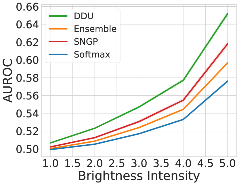
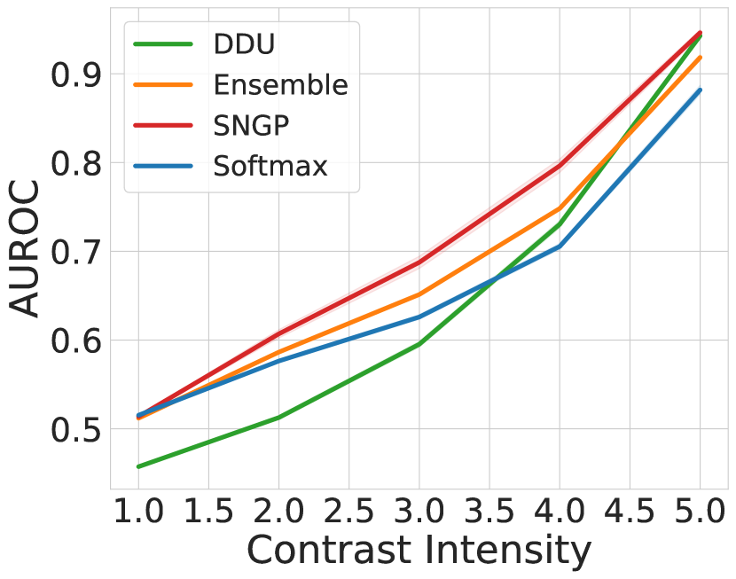
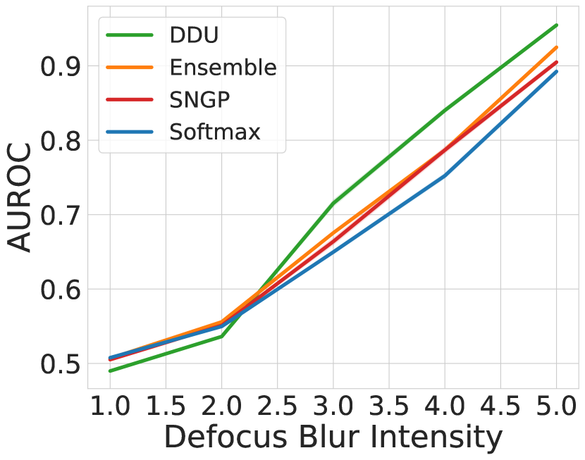
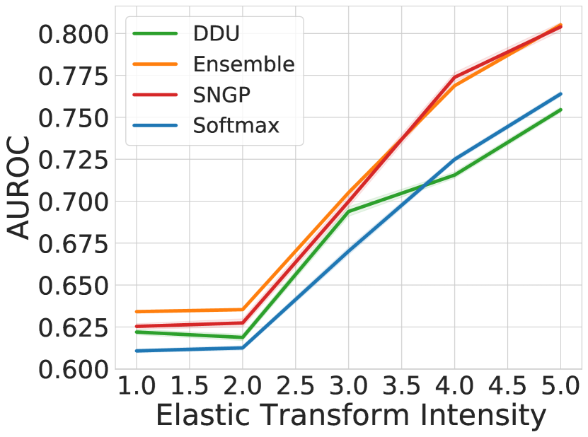
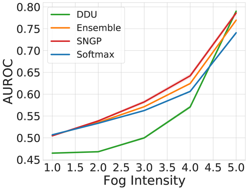
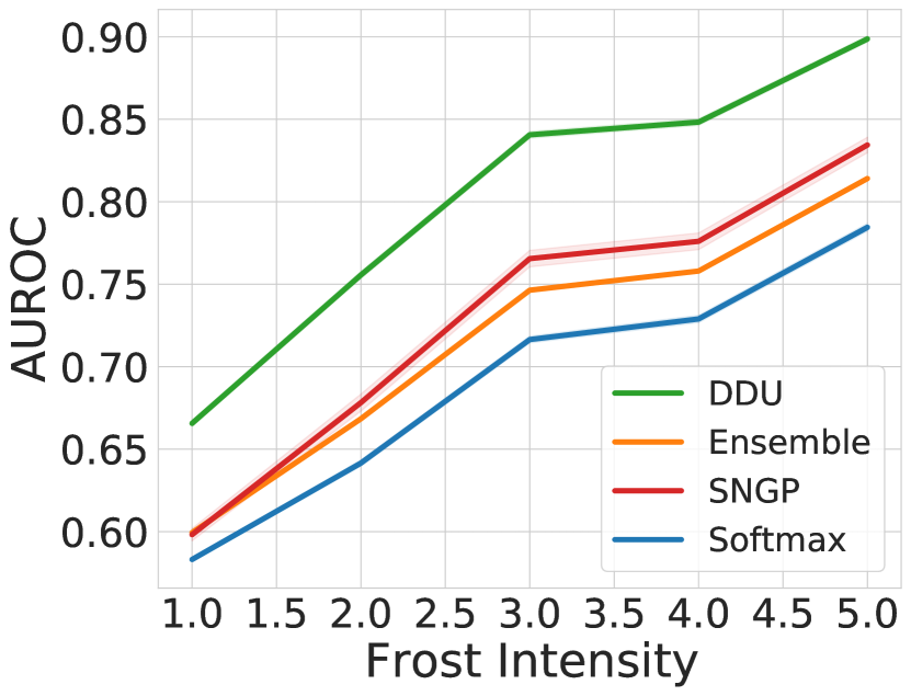
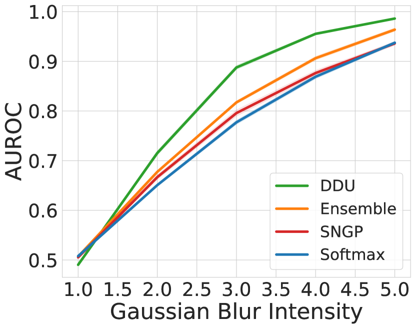
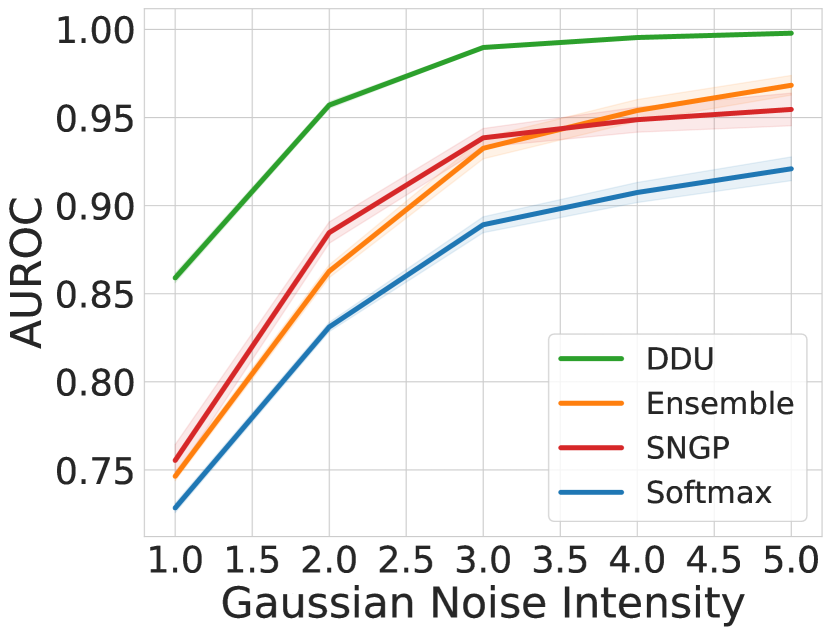
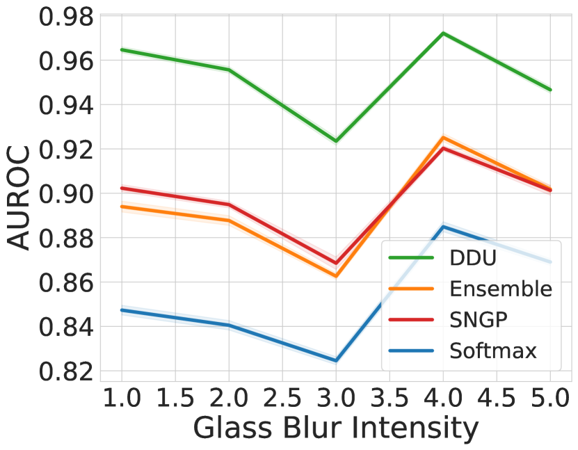
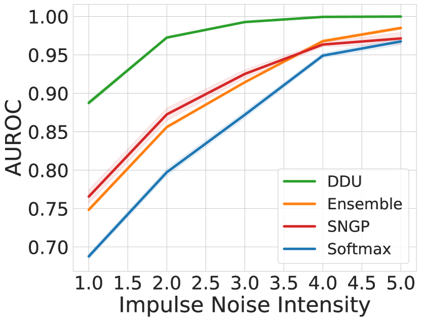
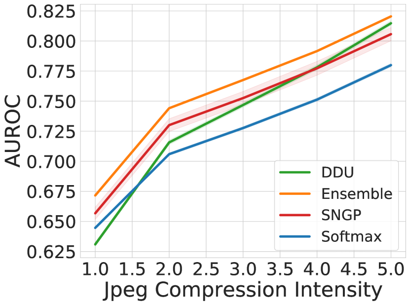
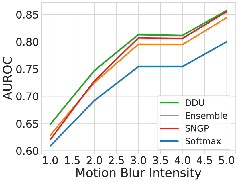
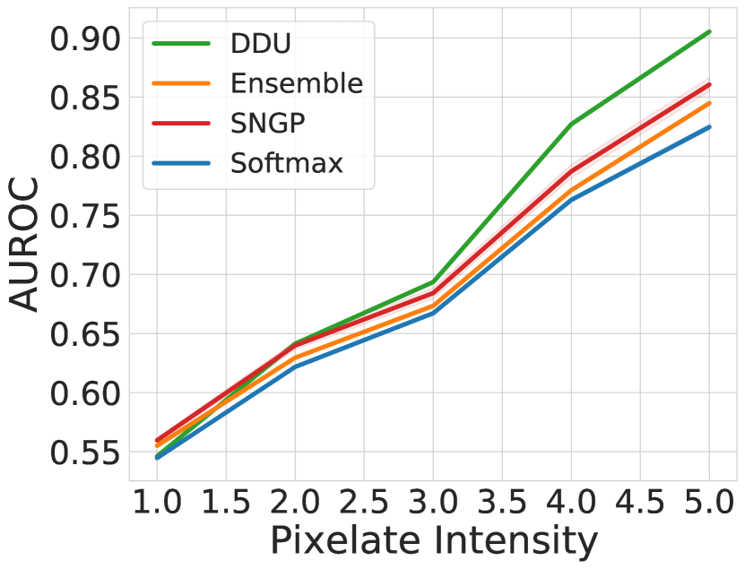
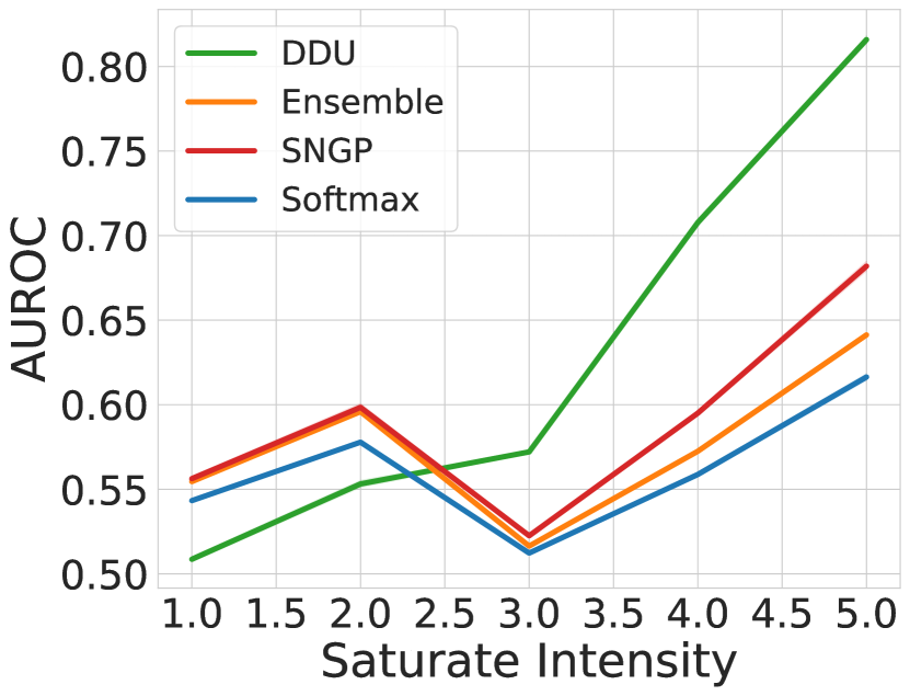
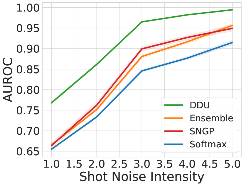
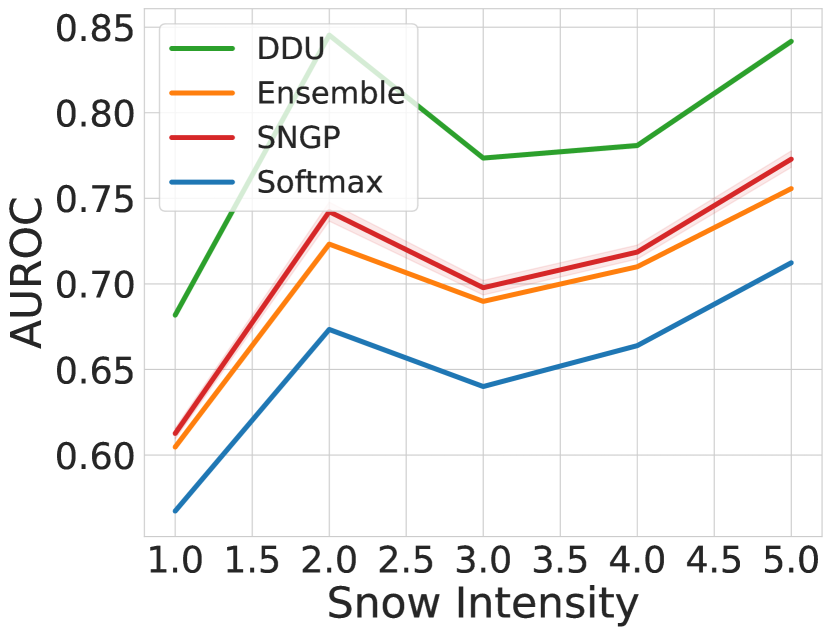
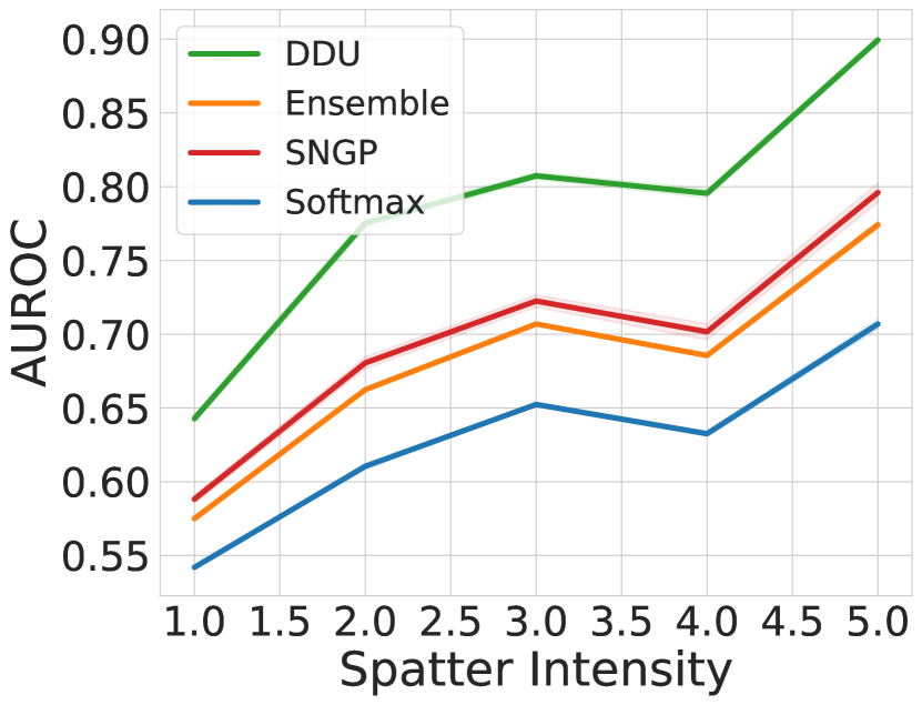
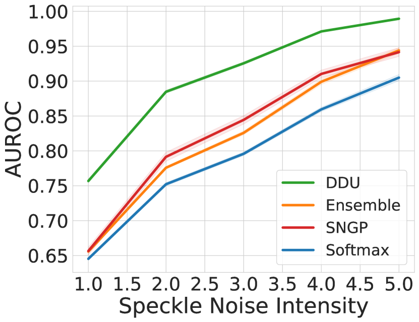
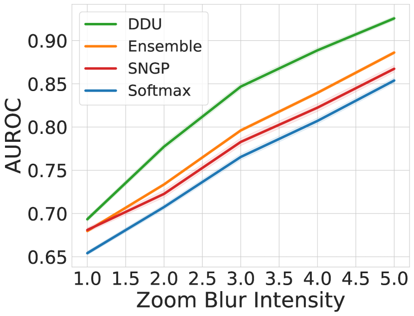
Figure 8: AUROC vs corruption intensity for all corruption types in CIFAR-10-C with Wide-ResNet-28-10 as the architecture and baselines: Softmax Entropy, Ensemble (using Predictive Entropy as uncertainty), SNGP and DDU feature density.

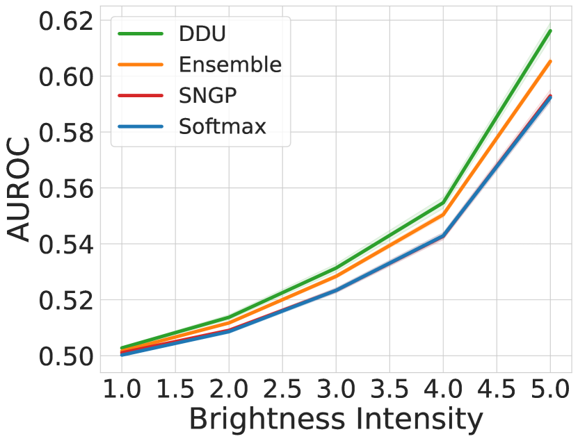
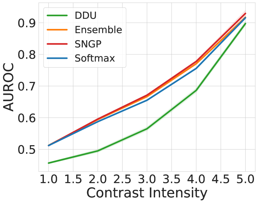
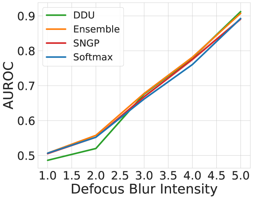
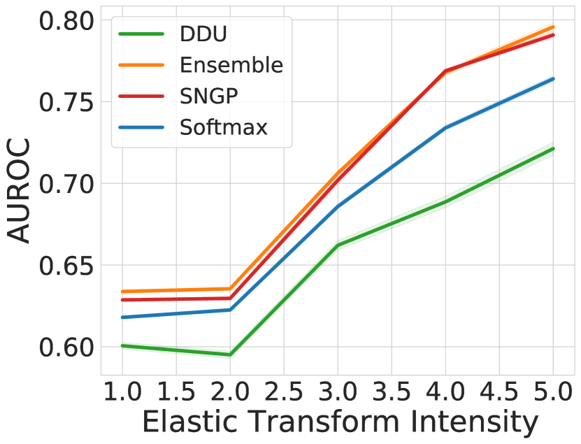
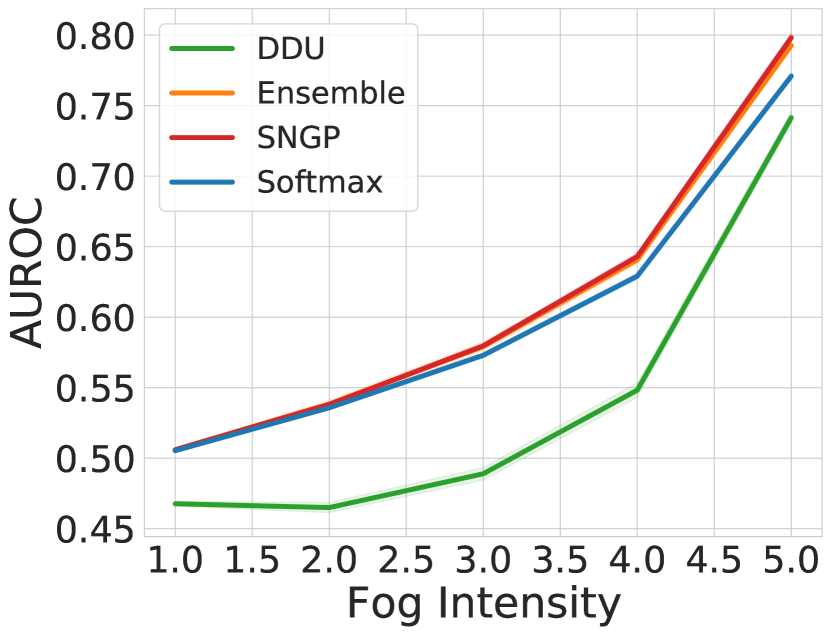
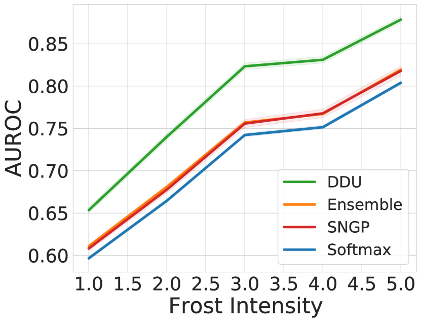
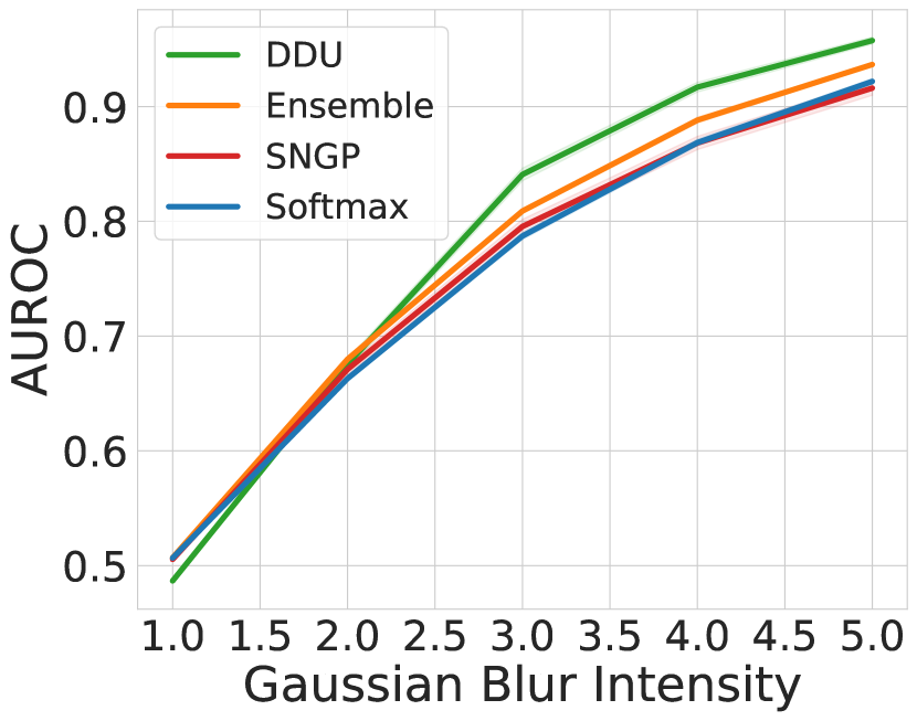
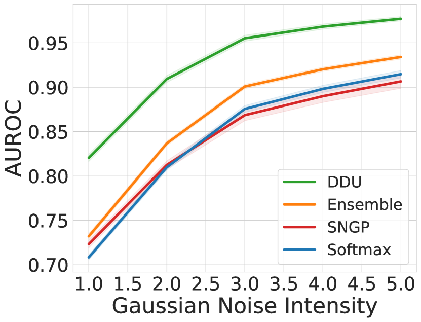
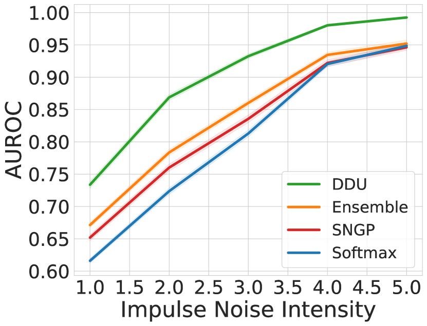
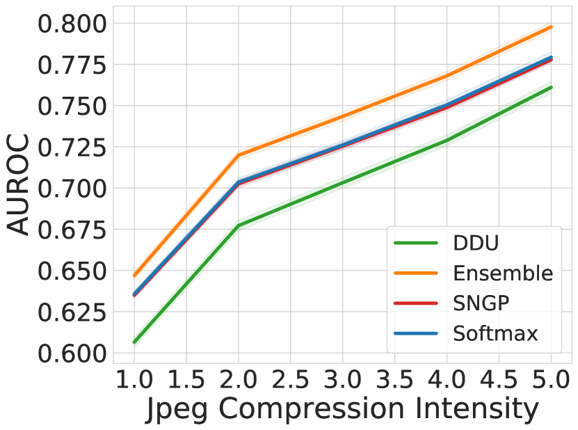
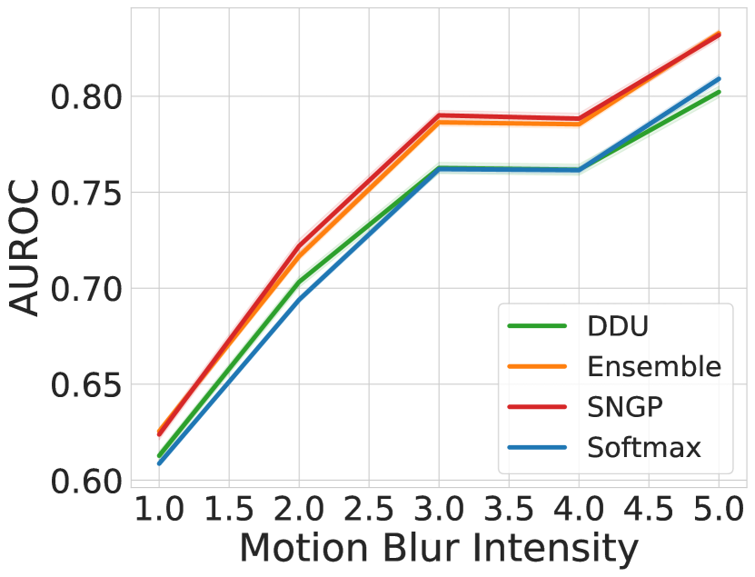
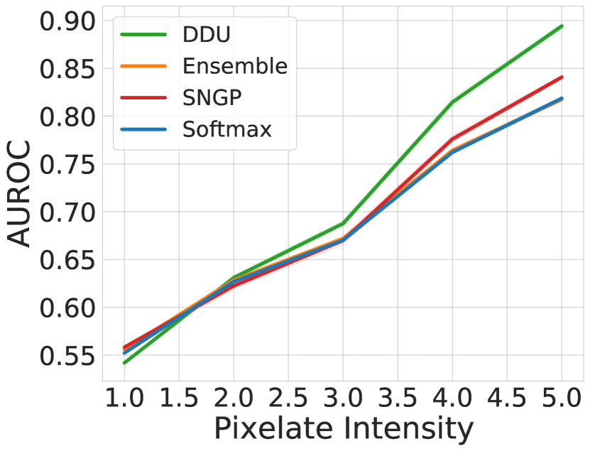
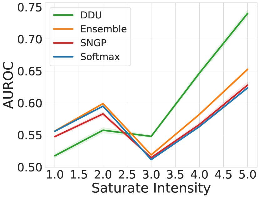
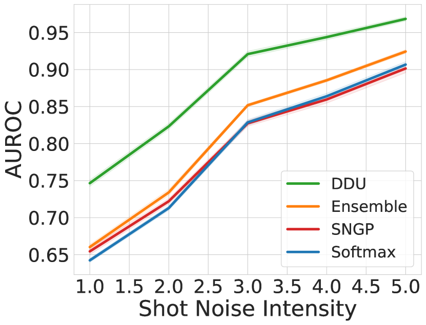
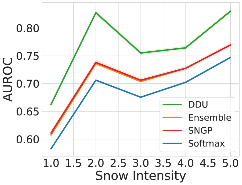
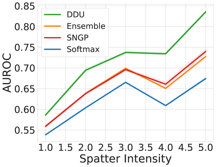
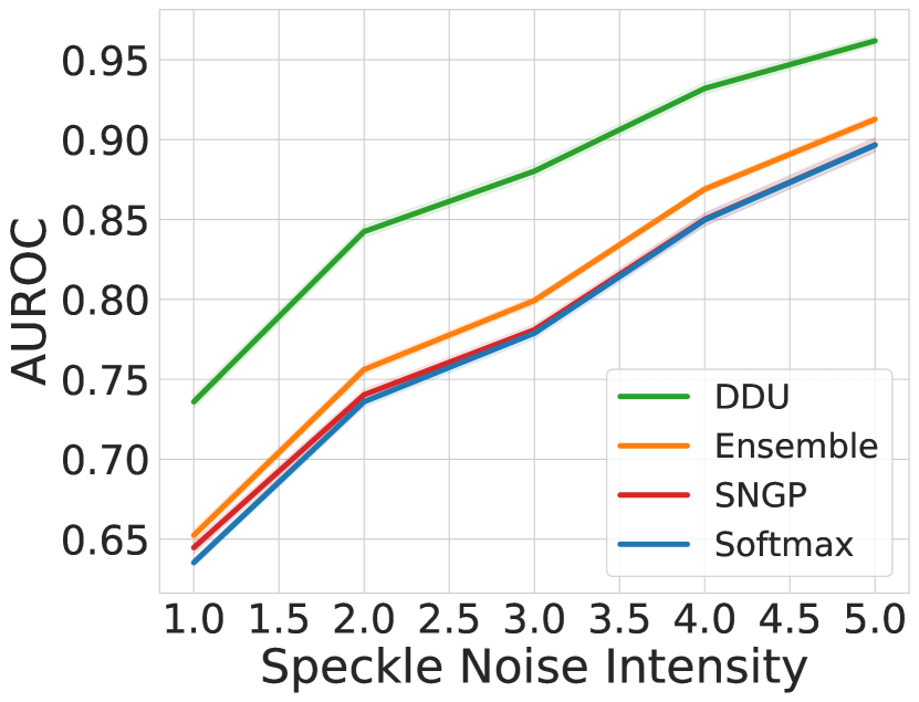
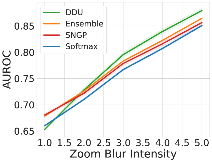
Figure 9: AUROC vs corruption intensity for all corruption types in CIFAR-10-C with ResNet-50 as the architecture and baselines: Softmax Entropy, Ensemble (using Predictive Entropy as uncertainty), SNGP and DDU feature density.

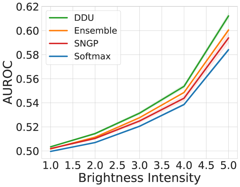
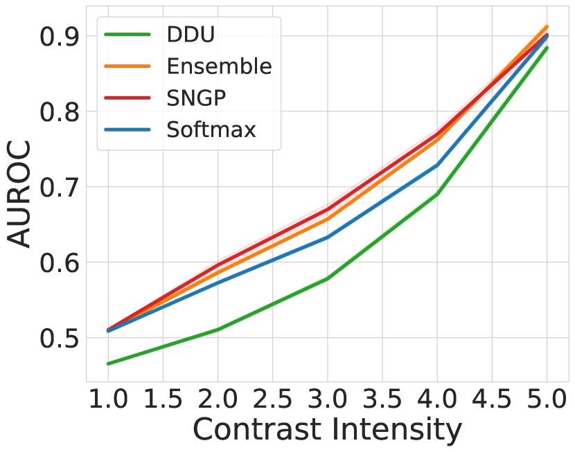
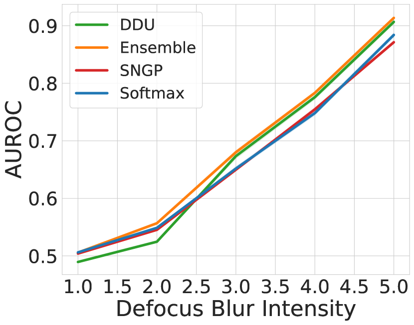
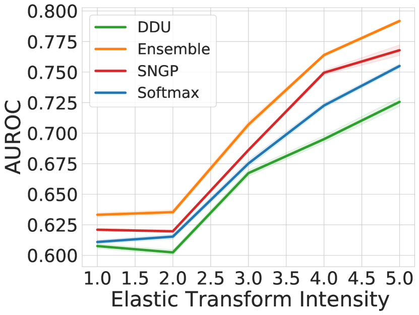
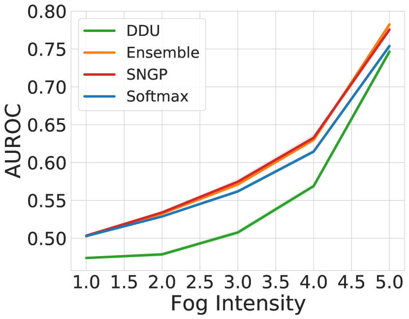
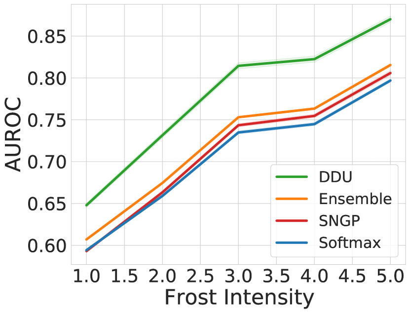
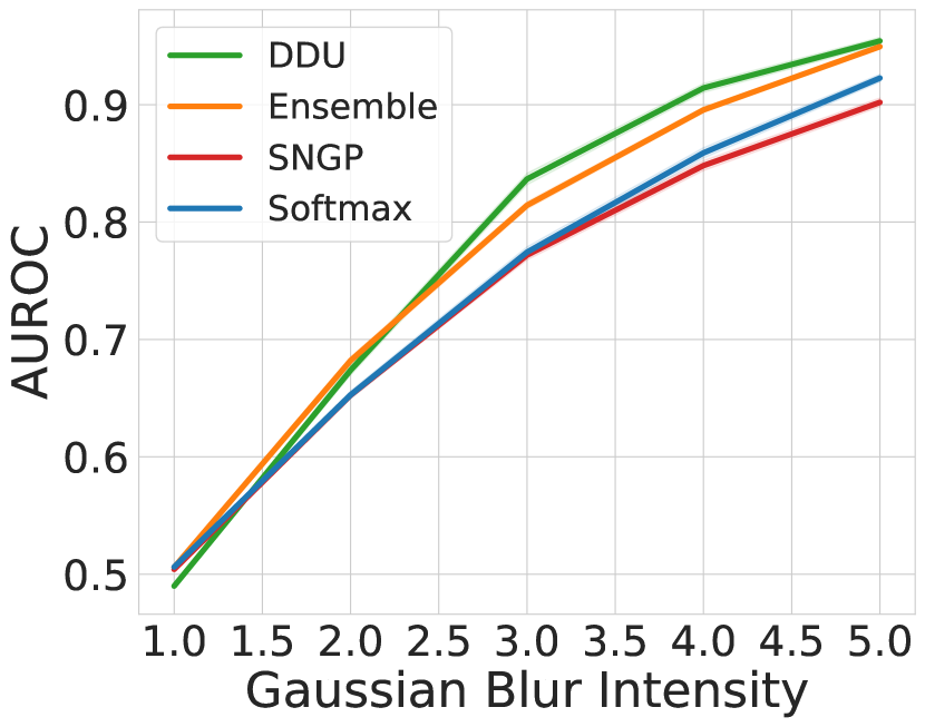
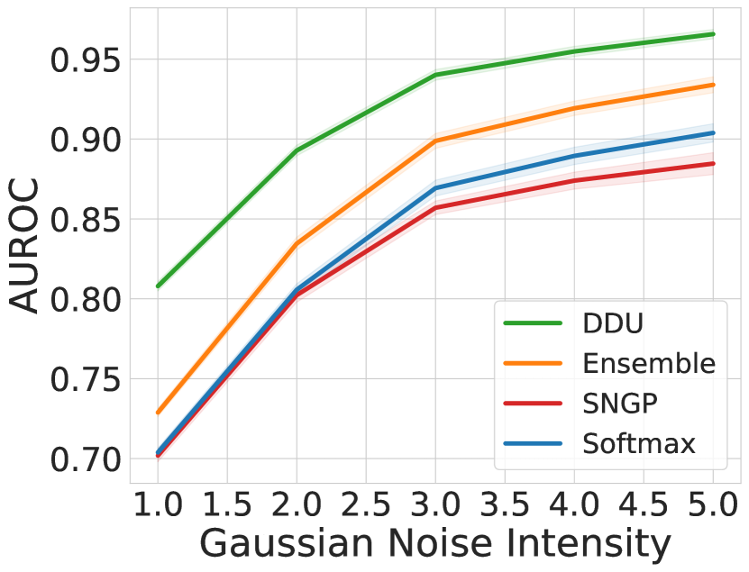
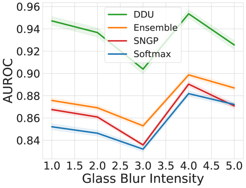
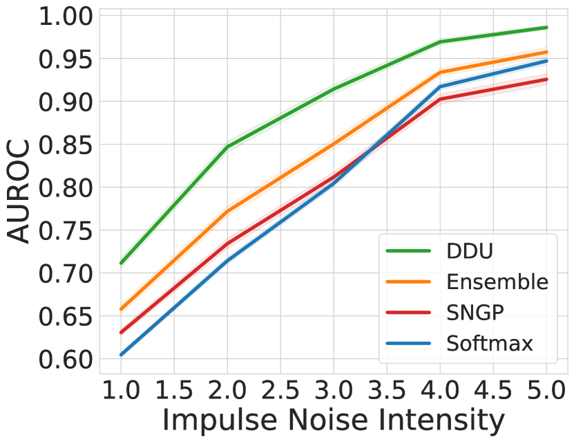
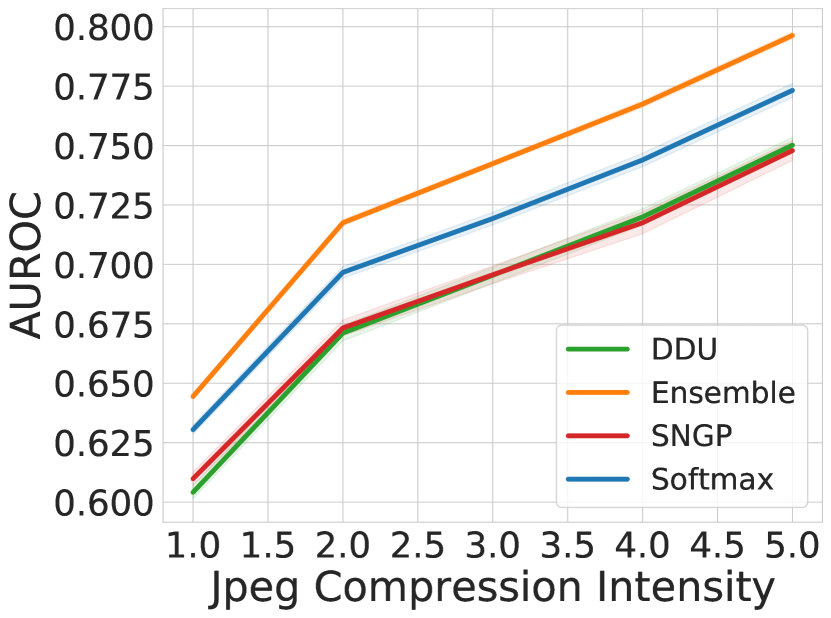
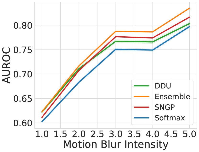
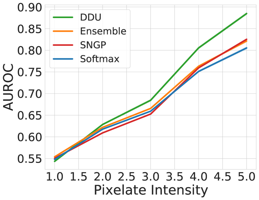
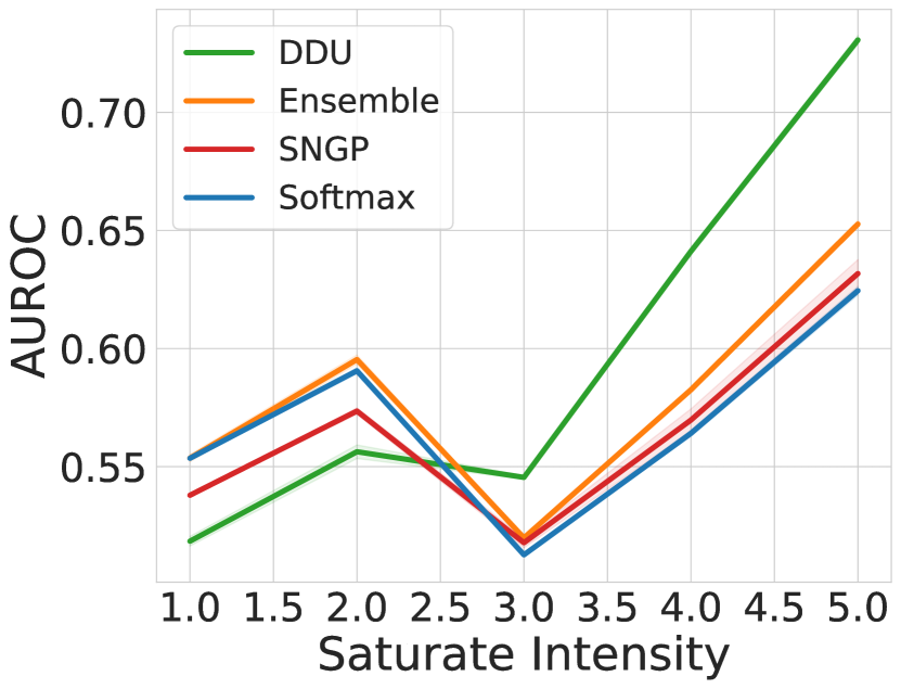
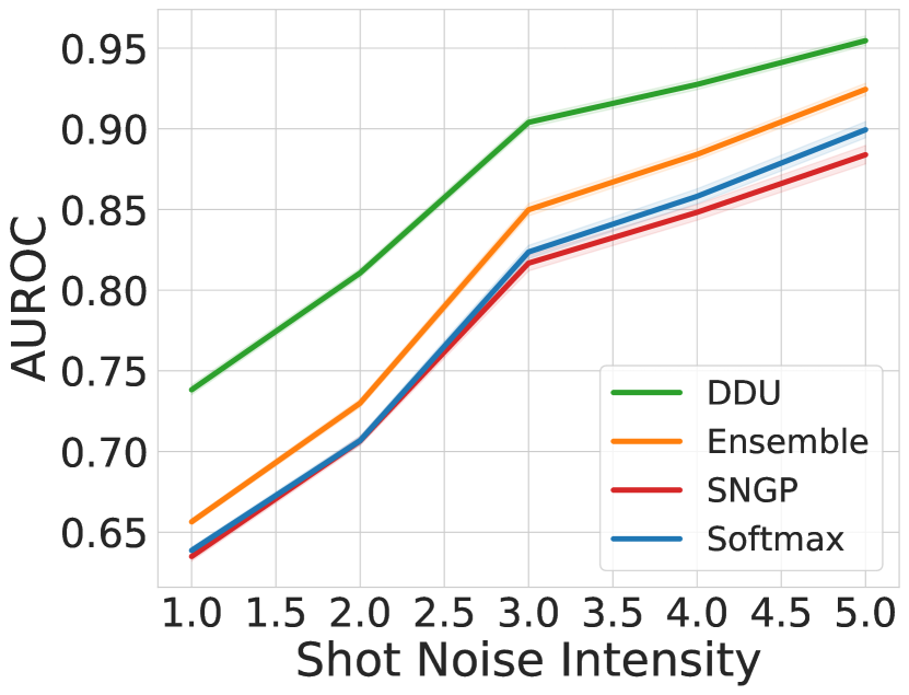
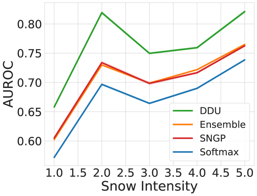
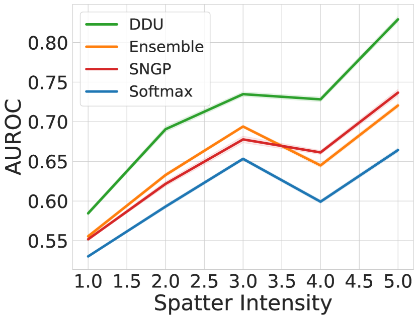
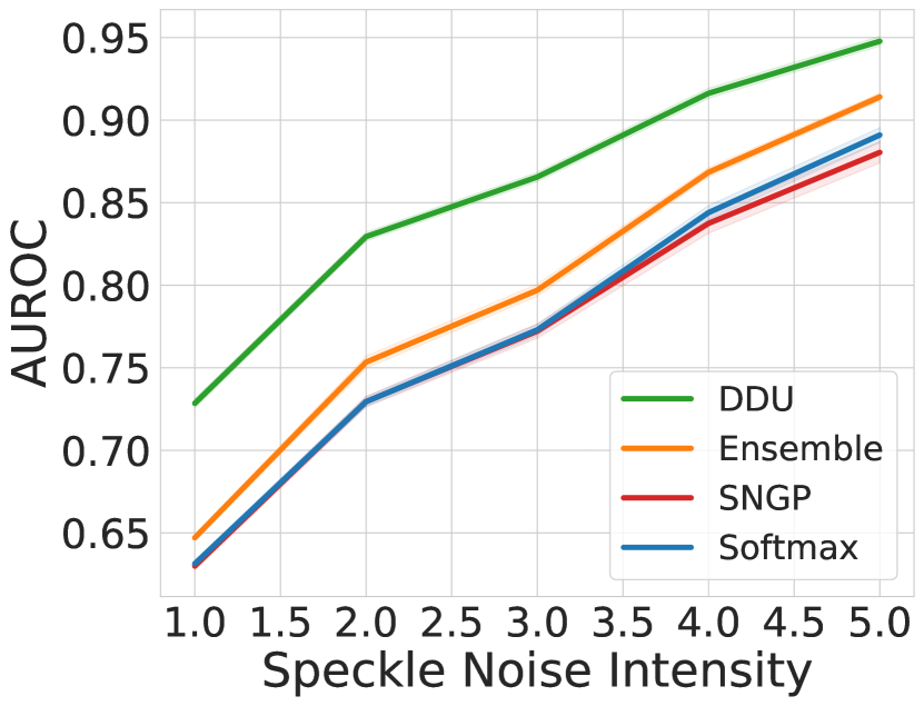
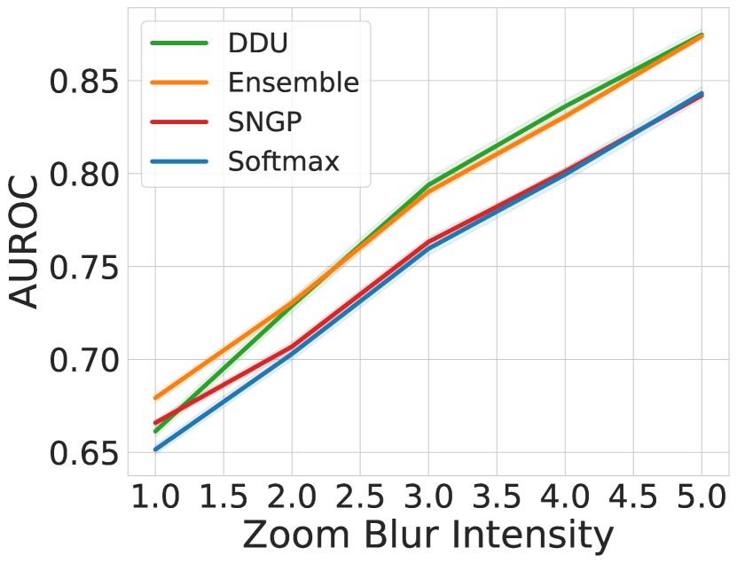
Figure 10: AUROC vs corruption intensity for all corruption types in CIFAR-10-C with ResNet-110 as the architecture and baselines: Softmax Entropy, Ensemble (using Predictive Entropy as uncertainty), SNGP and DDU feature density.

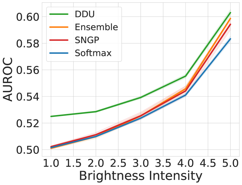
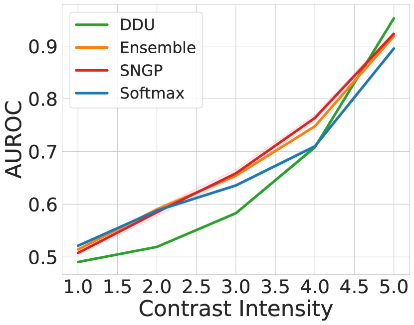
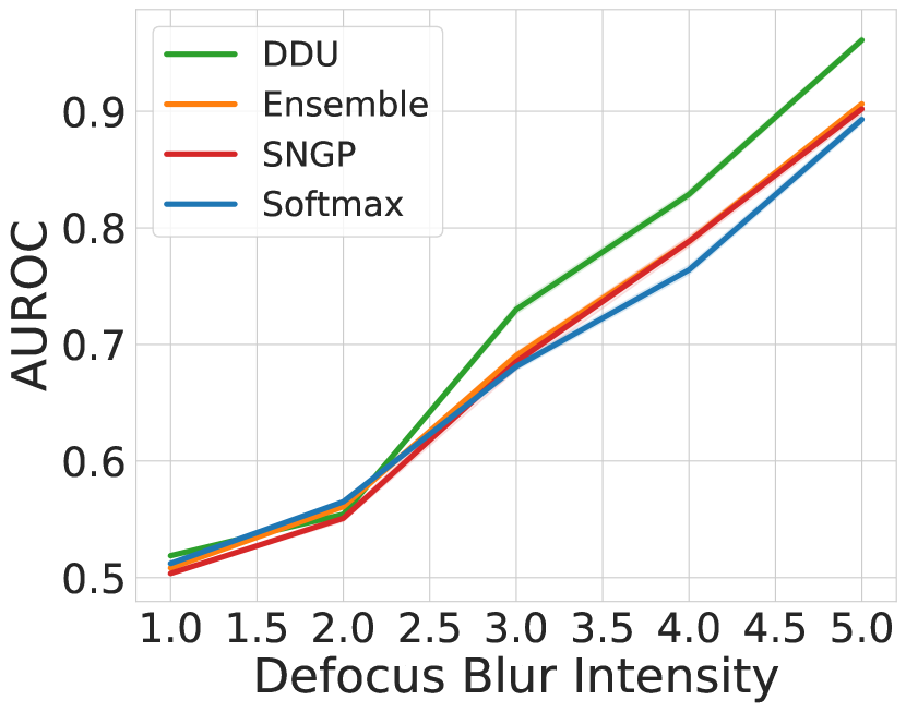
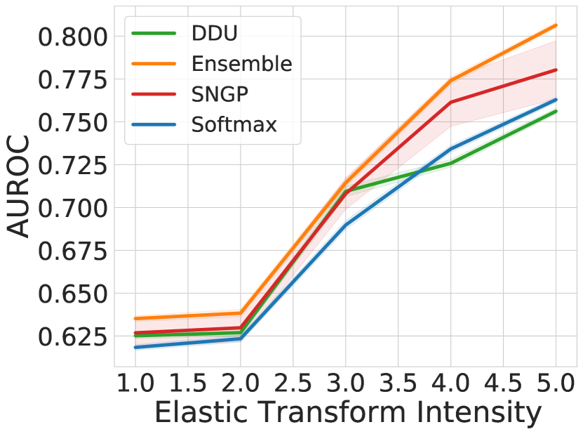
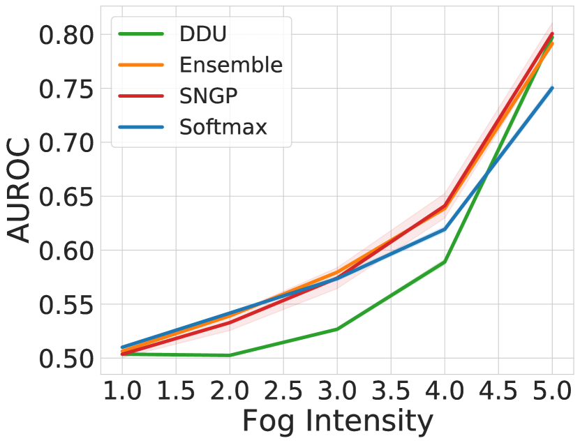
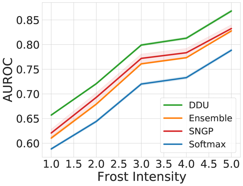
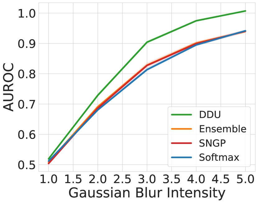
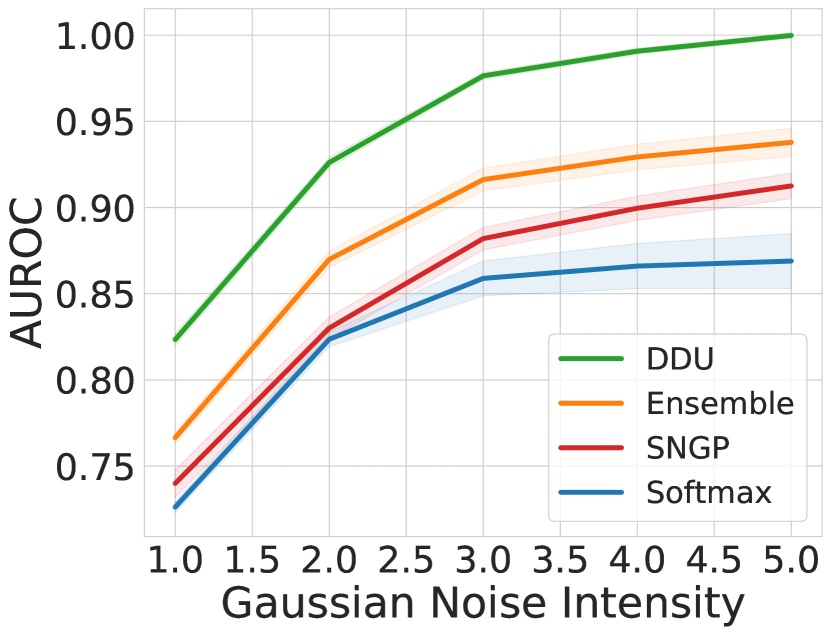
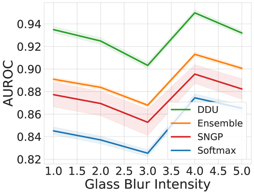
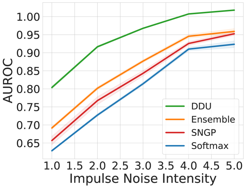
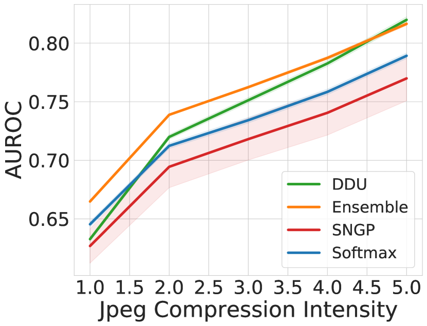
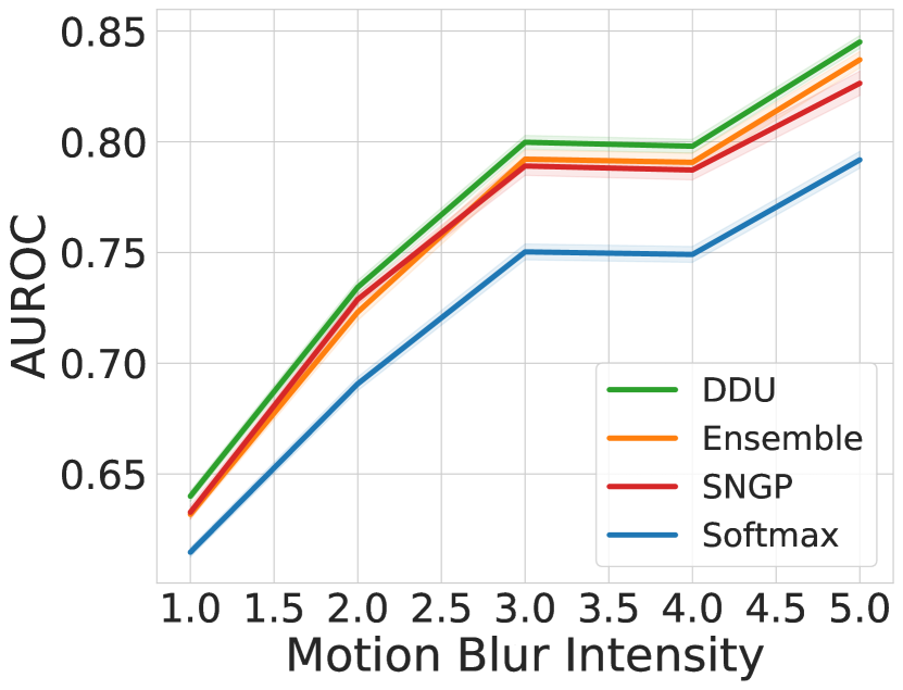
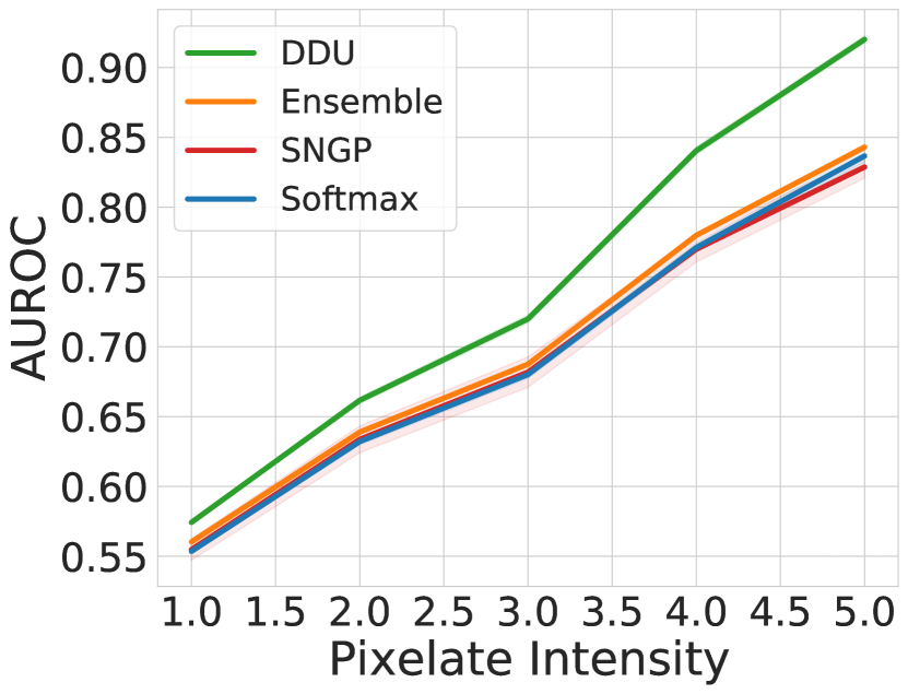
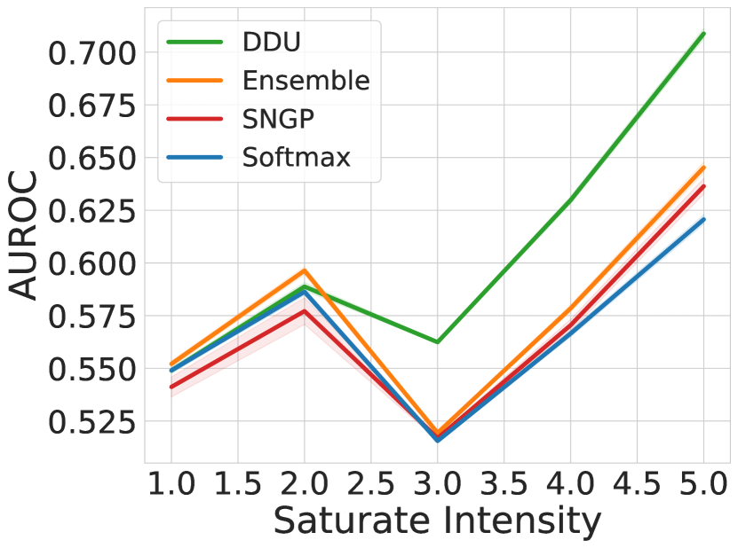
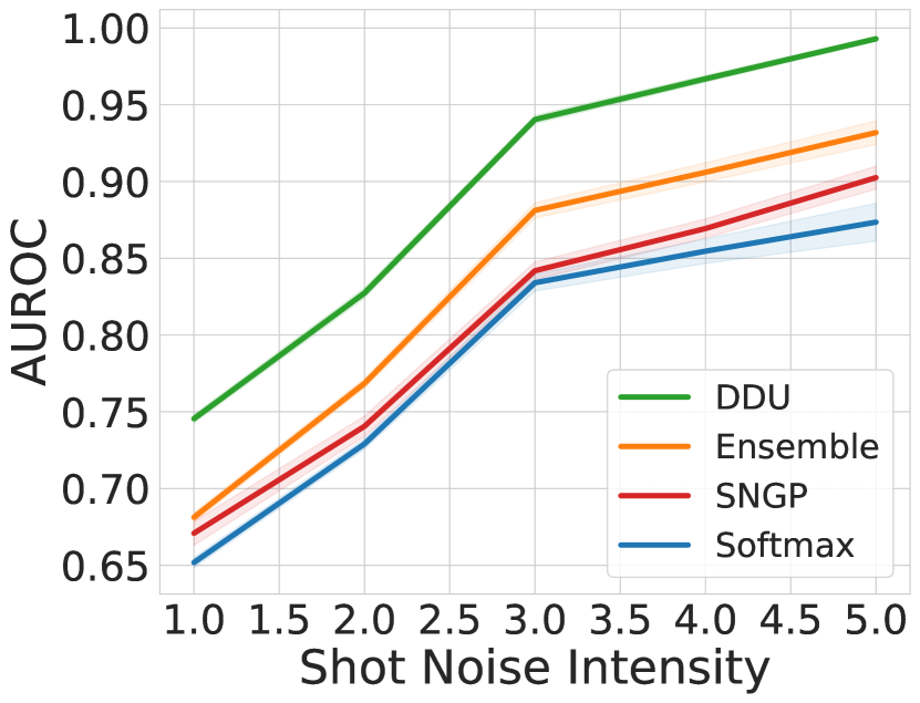
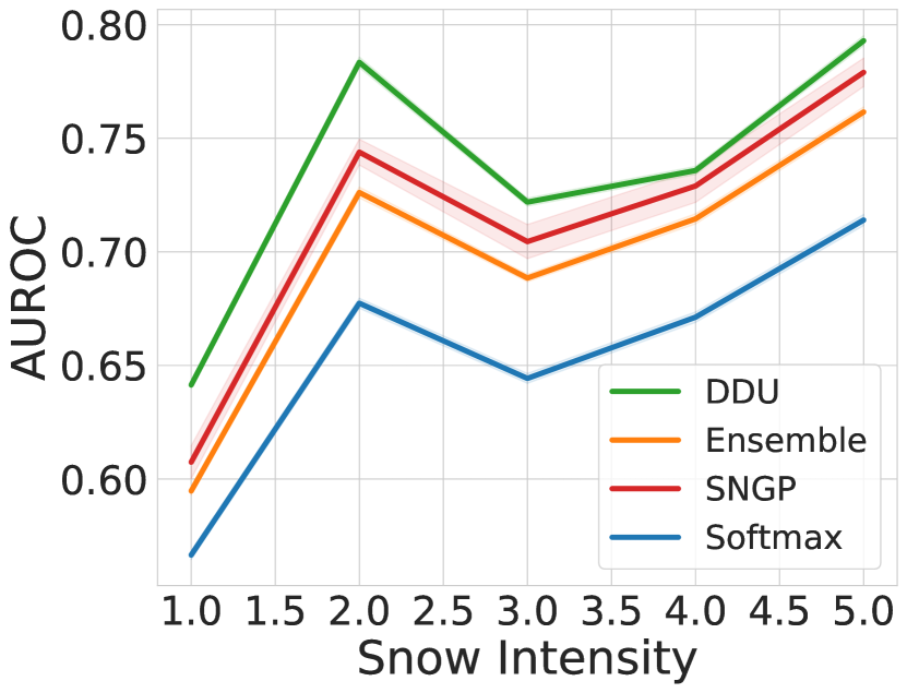
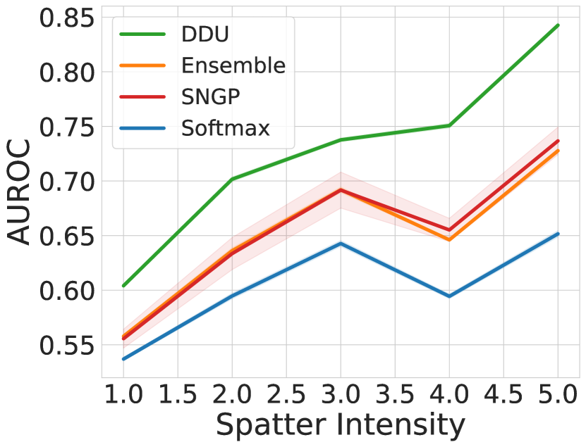
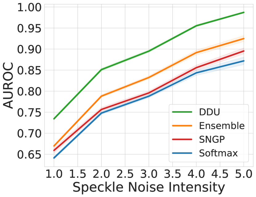
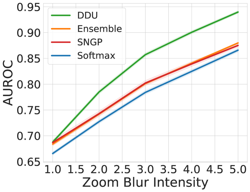
Figure 11: AUROC vs corruption intensity for all corruption types in CIFAR-10-C with DenseNet-121 as the architecture and baselines: Softmax Entropy, Ensemble (using Predictive Entropy as uncertainty), SNGP and DDU feature density.

Appendix E Additional Results

In this section, we provide details of additional results on the OoD detection task using CIFAR-10 vs SVHN/CIFAR-100/Tiny-ImageNet/CIFAR-10-C and CIFAR-100 vs SVHN/Tiny-ImageNet for ResNet-50, ResNet-110 and DenseNet-121 architectures. We present results on ResNet-50, ResNet-110 and DenseNet-121 for CIFAR-10 vs SVHN/CIFAR-100/Tiny-ImageNet and CIFAR-100 vs SVHN/Tiny-ImageNet in Table 4, Table 5 and Table 6 respectively. We also present results on individual corruption types for CIFAR-10-C for Wide-ResNet-28-10, ResNet-50, ResNet-110 and DenseNet-121 in Figure 8, Figure 9, Figure 10 and Figure 11 respectively.

Finally, we provide results for various ablations on DDU. As mentioned in §3, DDU consists of a deterministic softmax model trained with appropriate inductive biases. It uses softmax entropy to quantify aleatoric uncertainty and feature-space density to quantify epistemic uncertainty. In the ablation, we try to experimentally evaluate the following scenarios:

1. Effect of inductive biases (sensitivity + smoothness): We want to see the effect of removing the proposed inductive biases (i.e. no sensitivity and smoothness constraints) on the OoD detection performance of a model. To do this, we train a VGG-16 with and without spectral normalisation. Note that VGG-16 does not have residual connections and hence, a VGG-16 does not follow the sensitivity and smoothness (bi-Lipschitz) constraints.

2. Effect of sensitivity alone: Since residual connections make a model sensitive to changes in the input space by lower bounding its Lipschitz constant, we also want to see how a network performs with just the sensitivity constraint alone. To observe this, we train a Wide-ResNet-28-10 without spectral normalisation (i.e. no explicit upper bound on the Lipschitz constant of the model).

3. Metrics for aleatoric and epistemic uncertainty: With the above combinations, we try to observe how different metrics for aleatoric and epistemic uncertainty perform. To quantify aleatoric uncertainty, we use the softmax entropy of the model. On the other hand, to quantify the epistemic uncertainty, we use i) the softmax entropy, ii) the softmax density (Liu et al., 2020b) or iii) the GMM feature density (as described in §3).

For the purposes of comparison, we also present scores obtained by a 5-Ensemble of the respective architectures (i.e. Wide-ResNet-28-10 and VGG-16) in Table 7 for CIFAR-10 vs SVHN/CIFAR-100 and in Table 8 for CIFAR-100 vs SVHN. Based on these results, we can make the following observations (in addition to the ones we make in §4.2):

Inductive biases are important for feature density. From the AUROC scores in Table 7, we can see that using the feature density of a GMM in VGG-16 without the proposed inductive biases yields significantly lower AUROC scores as compared to Wide-ResNet-28-10 with inductive biases. In fact, in none of the datasets is the feature density of a VGG able to outperform its corresponding ensemble. This provides yet more evidence (in addition to Figure 2) to show that the GMM feature density alone cannot estimate epistemic uncertainty in a model that suffers from feature collapse. We need sensitivity and smoothness conditions (see §5) on the feature space of the model to obtain feature densities that capture epistemic uncertainty.

Sensitivity creates a bigger difference than smoothness. We note that the difference between AUROC obtained from feature density between Wide-ResNet-28-10 models with and without spectral normalisation is minimal. Although Wide-ResNet-28-10 with spectral normalisation (i.e. smoothness constraints) still outperforms its counterpart without spectral normalisation, the small difference between the AUROC scores indicates that it might be the residual connections (i.e. sensitivity constraints) that make the model detect OoD samples better. This observation is also intuitive as a sensitive feature extractor should map OoD samples farther from iD ones.

DDU as a simple baseline. In DDU, we use the softmax output of a model to get aleatoric uncertainty. We use the GMM’s feature-density to estimate the epistemic uncertainty. Hence, DDU does not suffer from miscalibration as the softmax outputs can be calibrated using post-hoc methods like temperature scaling. At the same time, the feature-densities of the model are not affected by temperature scaling and capture epistemic uncertainty well.

Appendix F Toy Experiments & Additional Ablations

Here, we provide details for toy experiments from the main paper which are visualized in Figure 2, Figure 4 and Figure 4.

F.1 Motivational Example in Figure 2

Table 9: ECE for Dirty-MNIST test set and AUROC for Dirty-MNIST vs Fashion-MNIST as proxies for aleatoric and epistemic uncertainty quality respectively.

Model	ECE	AUROC for Softmax Entropy ($\uparrow$)	AUROC for Feature Density ($\uparrow$)
LeNet	$2.22$	$84.23$	$71.41$
VGG-16	$\mathbf{2.11}$	$84.04$	$89.01$
ResNet-18+SN (DDU)	$2.34$	$83.01$	$\mathbf{99.91}$

In Figure 2 we train a LeNet (LeCun et al., 1998), a VGG-16 (Simonyan & Zisserman, 2015) and a ResNet-18 with spectral normalisation (He et al., 2016; Miyato et al., 2018) (ResNet-18+SN) on Dirty-MNIST, a modified version of MNIST (LeCun et al., 1998) with additional ambiguous digits (Ambiguous-MNIST). Ambiguous-MNIST contains samples with multiple plausible labels and thus higher aleatoric uncertainty (see Figure 2(a)). We refer to §B for details on how this dataset was generated. With ambiguous data having various levels of aleatoric uncertainty, Dirty-MNIST is more representative of real-world datasets compared to well-cleaned curated datasets, like MNIST and CIFAR-10, commonly used for benchmarking in ML (Filos et al., 2019; Krizhevsky et al., 2009). Moreover, Dirty-MNIST also poses a challenge for recent uncertainty estimation methods, which often confound aleatoric and epistemic uncertainty (van Amersfoort et al., 2020). Figure 2(b) shows that the softmax entropy of a deterministic model is unable to distinguish between iD (Dirty-MNIST) and OoD (Fashion-MNIST (Xiao et al., 2017)) samples as the entropy for the latter heavily overlaps with the entropy for Ambiguous-MNIST samples. However, the feature-space density of the model with our inductive biases in Figure 2(c) captures epistemic uncertainty reliably and is able to distinguish iD from OoD samples. The same cannot be said for LeNet or VGG in Figure 2(c), whose densities are unable to separate OoD from iD samples. This demonstrates the importance of the inductive bias to ensure the sensitivity and smoothness of the feature space as we further argue below. Finally, Figure 2(b) and Figure 2(c) demonstrate that our method is able to separate aleatoric from epistemic uncertainty: samples with low feature density have high epistemic uncertainty, whereas those with both high feature density and high softmax entropy have high aleatoric uncertainty—note the high softmax entropy for the most ambiguous Ambiguous-MNIST samples in Figure 2(b).

F.1.1 Disentangling Epistemic and Aleatoric Uncertainty

We used a simple example in §1 to demonstrate that a single softmax model with a proper inductive bias can reliably capture epistemic uncertainty via its feature-space density and aleatoric uncertainty via its softmax entropy. To recreate the natural characteristics of uncurated real-world datasets, which contain ambiguous samples, we use MNIST (LeCun et al., 1998) as an iD dataset of unambiguous samples, Ambiguous-MNIST as an iD dataset of ambiguous samples and Fashion-MNIST (Xiao et al., 2017) as an OoD dataset (see Figure 2(a)), with more details in §B. We train a LeNet (LeCun et al., 1998), a VGG-16 (Simonyan & Zisserman, 2015) and a ResNet-18 (He et al., 2016) with spectral normalisation (SN) on Dirty-MNIST (a mix of Ambiguous- and standard MNIST) with the training setup detailed in §D.1.

Table 9 gives a quantitative evaluation of the qualitative results in §1. The AUROC metric reflects the quality of the epistemic uncertainty as it measures the probability that iD and OoD samples can be distinguished, and OoD samples are never seen during training while iD samples are semantically similar to training samples. The ECE metric measures the quality of the aleatoric uncertainty. The softmax outputs capture aleatoric uncertainty well, as expected, and all 3 models obtain similar ECE scores on the Dirty-MNIST test set. However, with an AUROC of around $84\%$ for all the 3 models, on Dirty-MNIST vs Fashion-MNIST, we conclude that softmax entropy is unable to capture epistemic uncertainty well. This is reinforced in Figure 2(b), which shows a strong overlap between the softmax entropy of OoD and ambiguous iD samples. At the same time, the feature-space densities of LeNet and VGG-16, with AUROC scores around $71\%$ and $89\%$ respectively, are unable to distinguish OoD from iD samples, indicating that simply using feature-space density without appropriate inductive biases (as seen in (Lee et al., 2018b)) is not sufficient.

Only by fitting a GMM on top of a feature extractor with appropriate inductive biases (DDU) and using its feature density are we able to obtain performance far better (with AUROC of $99.9\%$) than the alternatives in the ablation study (see Table 9, also noticeable in Figure 2(c)). The entropy of a softmax model can capture aleatoric uncertainty, even without additional inductive biases, but it cannot be used to estimate epistemic uncertainty (see §5). On the other hand, feature-space density can only be used to estimate epistemic uncertainty when the feature extractor is sensitive and smooth, as achieved by using a ResNet and spectral normalisation in DDU.

F.2 Effects of a well-regularized feature space on feature collapse

The effects of a well-regularized feature space on feature collapse are visible in Figure 2. In the case of feature collapse, we must have some OoD inputs for which the features are mapped on top of the features of iD inputs. The distances of these OoD features to each class centroid must be equal to the distances of the corresponding iD inputs to class centroids, and hence the density for these OoD inputs must be equal to the density of the iD inputs. If the density histograms do not overlap, no feature collapse can be present. We see no overlapping densities in Figure 2(c, right), therefore we indeed have no feature collapse. First, the effects of having a well-regularized feature space on feature collapse can be analysed from Figure 2. In case of feature collapse we must have some OoD features mapped ontop of iD features, therefore the distances of at least some OoD features to the class centroids must be equal to iD’s distances, hence OoD density must overlap with iD density. We see this in Figure 2(c) (left) in the case without a regularized feature space. On the other hand, when we regularize the feature space, we see the densities do not overlap, i.e. the distances of the features of OoD examples to the centroids are larger than the distances of iD examples (Figure 2(c) right), hence feature collapse is not present.

F.3 Two Moons

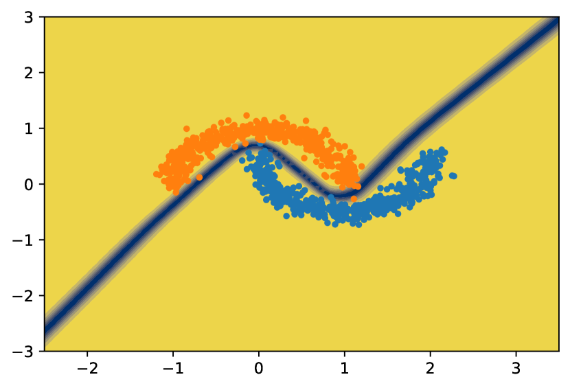
(a) Softmax Entropy

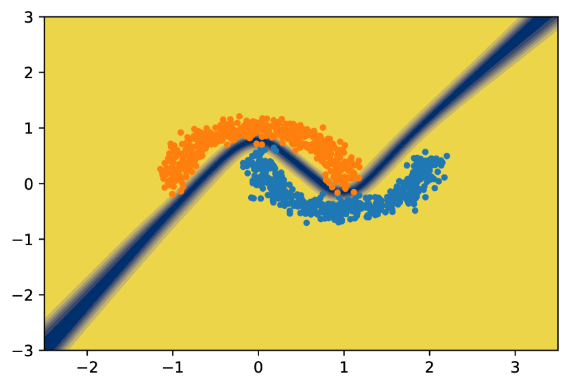
(b) Ensemble Predictive Entropy

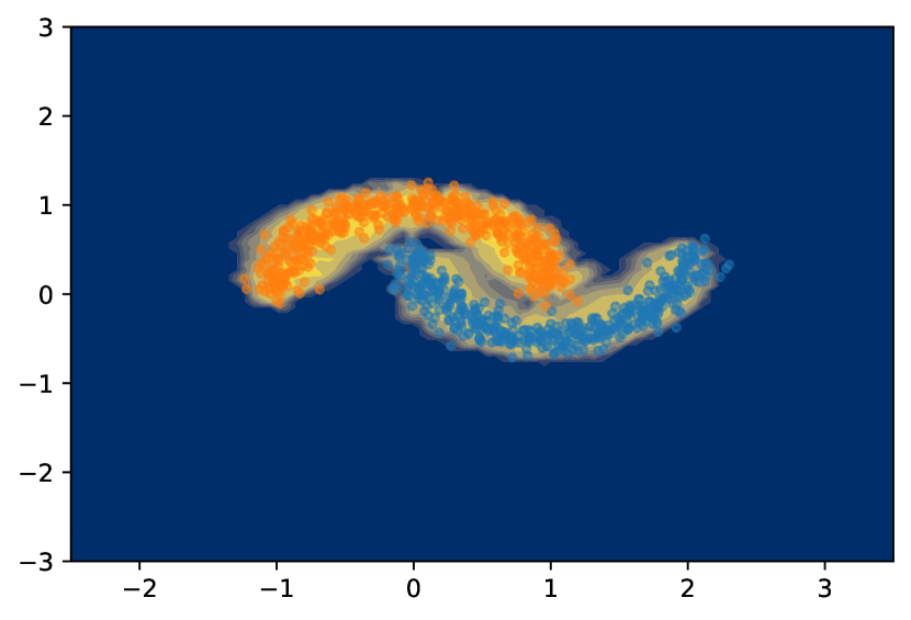
(c) DDU Feature-space density

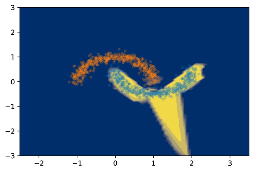
(d) FC-Net Feature-space density

Figure 12: Uncertainty on Two Moons dataset. Blue indicates high uncertainty and yellow indicates low uncertainty. Both the softmax entropy of a single model as well as the predictive entropy of a deep ensemble are uncertain only along the decision boundary whereas the feature-space density of DDU is uncertain everywhere except on the data distribution (the ideal behaviour). However, the feature density of a normal fully connected network (FC-Net) without any inductive biases can’t capture uncertainty properly.

In this section, we evaluate DDU’s performance on a well-known toy setup: the Two Moons dataset. We use scikit-learn’s datasets package to generate 2000 samples with a noise rate of 0.1. We use a 4-layer fully connected architecture, ResFFN-4-128 with 128 neurons in each layer and a residual connection, following (Liu et al., 2020a). As an ablation, we also train using a 4-layer fully connected architecture with 128 neurons in each layer, but without the residual connection. We name this architecture FC-Net. The input is 2-dimensional and is projected into the 128 dimensional space using a fully connected layer. Using the ResFFN-4-128 architecture we train 3 baselines:

1. Softmax: We train a single softmax model and use the softmax entropy as the uncertainty metric.

2. 3-ensemble: We train an ensemble of 3 softmax models and use the predictive entropy of the ensemble as the measure of uncertainty.

3. DDU: We train a single softmax model applying spectral normalization on the fully connected layers and using the feature density as the measure of model confidence.

Each model is trained using the Adam optimiser for 150 epochs. In Figure 12, we show the uncertainty results for all the above 3 baselines. It is clear that both the softmax entropy as well as the predictive entropy of the ensemble is uncertain only along the decision boundary between the two classes whereas DDU is confident only on the data distribution and is not confident anywhere else. It is worth mentioning that even DUQ and SNGP perform well in this setup and deep ensembles have been known to underperform in the Two-Moons setup primarily due to the simplicity of the dataset causing all the ensemble components to generalise in the same way. Finally, also note that the feature space density of FC-Net without residual connections is not able to capture uncertainty well (see Figure 12(d)), thereby reaffirming our claim that proper inductive biases are indeed a necessary component to ensure that feature space density captures uncertainty reliably. Thus, in addition to its excellent performance in active learning, CIFAR-10 vs SVHN/CIFAR-100/Tiny-ImageNet/CIFAR-10-C, CIFAR-100 vs SVHN/Tiny-ImageNet, and ImageNet vs ImageNet-O, we note that DDU captures uncertainty reliably even in a small 2D setup like Two Moons.

F.4 5-Ensemble Visualisation

In Figure 4, we provide a visualisation of a 5-ensemble (with five deterministic softmax networks) to see how softmax entropy fails to capture epistemic uncertainty precisely because the mutual information (MI) of an ensemble does not (see §5). We train the networks on 1-dimensional data with binary labels 0 and 1. The data is shown in Figure 3(a). From Figure 3(a) and Figure 3(b), we find that the softmax entropy is high in regions of ambiguity where the label can be both 0 and 1 (i.e. x between -4.5 and -3.5, and between 3.5 and 4.5). This indicates that softmax entropy can capture aleatoric uncertainty. Furthermore, in the x interval $(-2,2)$, we find that the deterministic softmax networks disagree in their predictions (see Figure 3(a)) and have softmax entropies which can be high, low or anywhere in between (see Figure 3(b)) following our claim in §5. In fact, this disagreement is the very reason why the MI of the ensemble is high in the interval $(-2,2)$, thereby reliably capturing epistemic uncertainty. Finally, note that the predictive entropy (PE) of the ensemble is high both in the OoD interval $(-2,2)$ as well as at points of ambiguity (i.e. at -4 and 4). This indicates that the PE of a Deep Ensemble captures both epistemic and aleatoric uncertainty well. From these visualisations, we draw the conclusion that the softmax entropy of a deterministic softmax model cannot capture epistemic uncertainty precisely because the MI of a Deep Ensemble can.

F.5 Feature-Space Density & Epistemic Uncertainty vs Softmax Entropy & Aleatoric Uncertainty

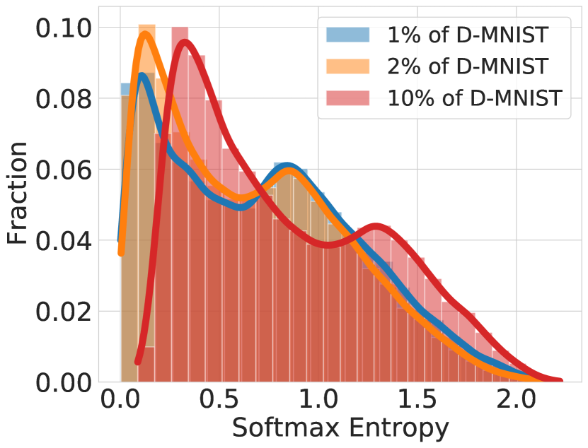
(a) SE D-MNIST

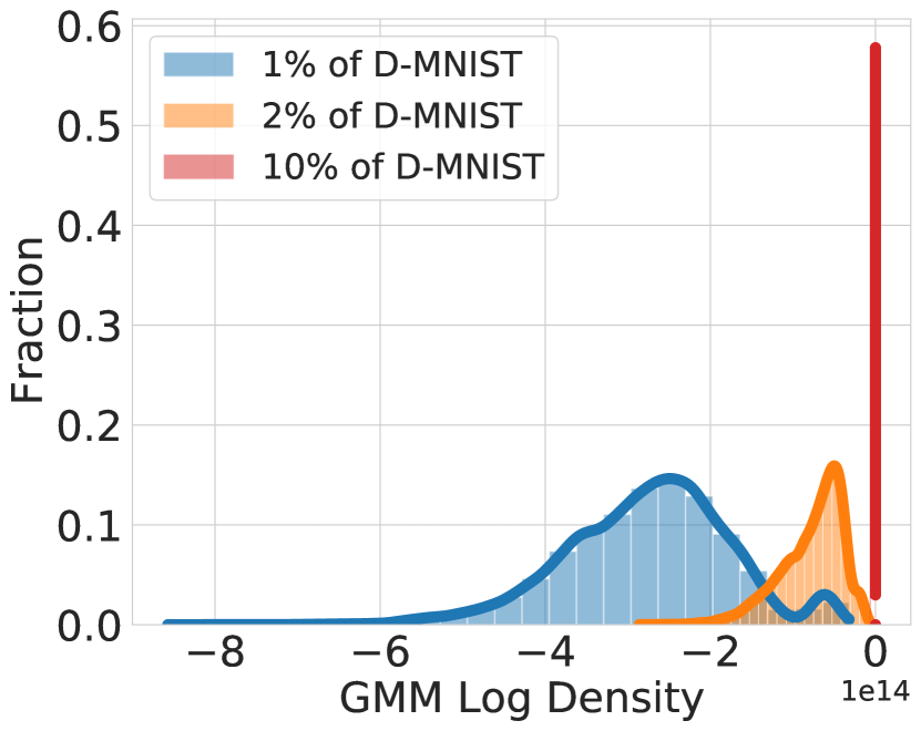
(b) Density D-MNIST

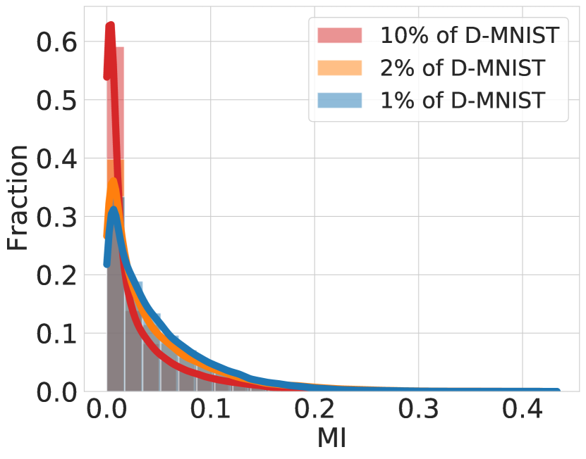
(c) MI D-MNIST

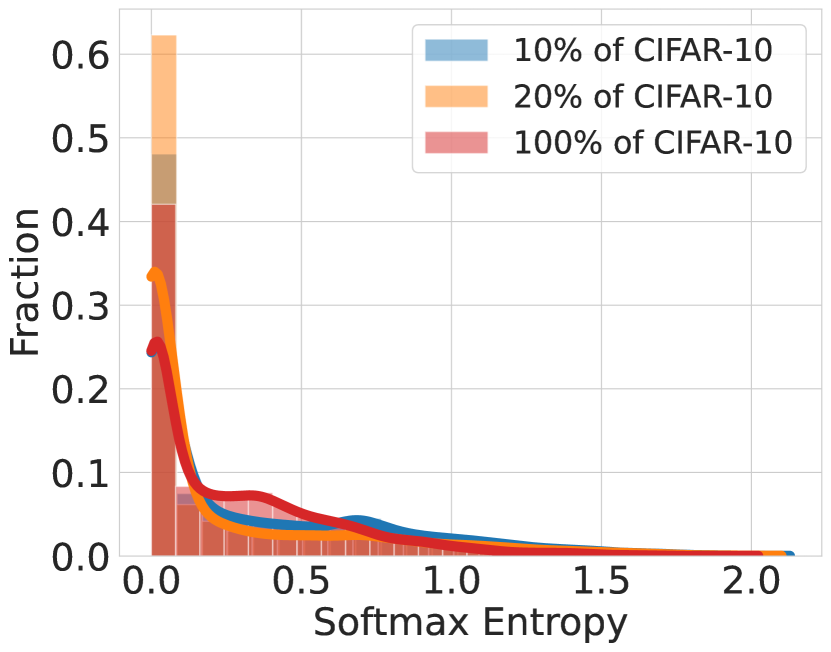
(d) SE CIFAR-10

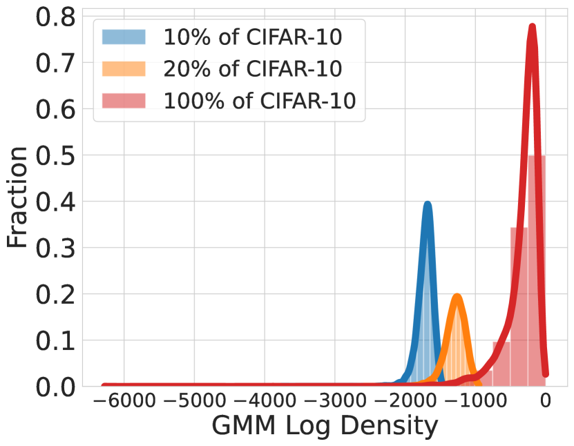
(e) Density CIFAR-10

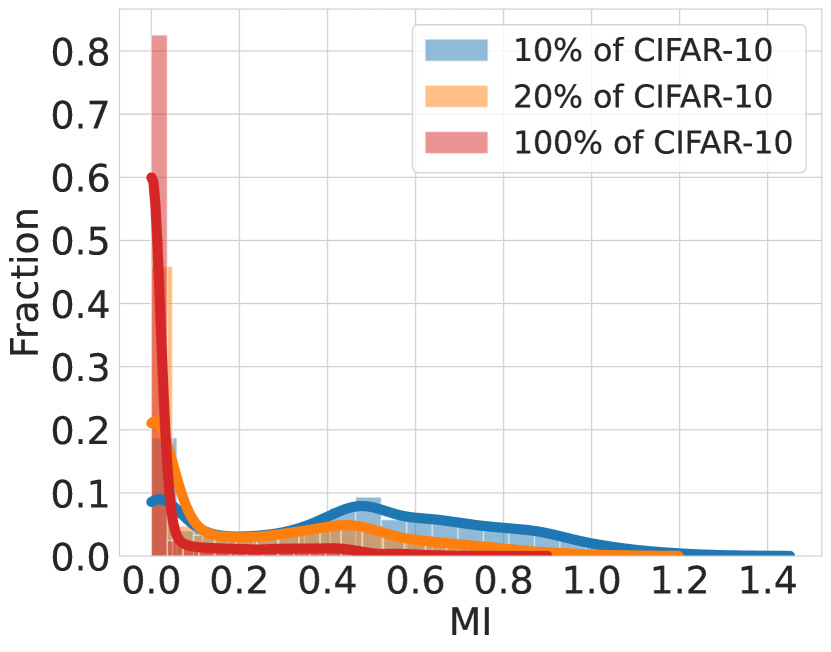
(f) MI CIFAR-10

Figure 13: Comparison of epistemic and aleatoric uncertainty captured b(ResNet-18+SN) on increasingly large subsets of Dirty-MNIST and CIFAR-10. Clearly, feature density captures epistemic uncertainty which reduces when the model is trained on increasingly large subsets of training data, whereas softmax entropy (SE) does not. For comparison, we also plot a deep-ensemble’s epistemic uncertainty, through mutual information (MI) for the same settings. For more details, see Table 10.

Table 10: Average softmax entropy (SE) and feature-space density of the test set for models trained on different amounts of the training set (Dirty-MNIST and CIFAR-10) behave consistently with aleatoric and epistemic uncertainty. Aleatoric uncertainty for individual samples does not change much as more data is added to the training set while epistemic uncertainty decreases as more data is added. This is also consistent with Table 3 in Kendall & Gal (2017). Finally, we observe a consistent strong positive correlation between the negative log feature space density and the mutual information (MI) of a deep ensemble trained on the same subsets of data for both Dirty-MNIST and CIFAR-10. However, the correlation between softmax entropy and MI is not consistent.

Training Set	Avg Test SE ($\boldmath\approx$)	Avg Test Log GMM Density ($\uparrow$)	Avg Test MI	Correlation(SE || MI)	Correlation(-Log GMM Density || MI)
1% of D-MNIST	$0.7407$	$-2.7268e+14$	$0.0476$	$-0.79897$	$0.8132$
2% of D-MNIST	$0.6580$	$-7.8633e+13$	$0.0447$
10% of D-MNIST	$0.8295$	$-1279.1753$	$0.0286$
10% of CIFAR-10	$0.3189$	$-1715.3516$	$0.4573$	$0.5663$	$0.9556$
20% of CIFAR-10	$0.2305$	$-1290.1726$	$0.2247$
100% of CIFAR-10	$0.2747$	$-324.8040$	$0.0479$

To empirically verify the connection between feature-space density and epistemic uncertainty on the one hand and the connection between softmax entropy and aleatoric uncertainty on the other hand, we train ResNet-18+SN models on increasingly large subsets of DirtyMNIST and CIFAR-10 and evaluate the epistemic and aleatoric uncertainty on the corresponding test sets using the feature-space density and softmax entropy, respectively. Moreover, we also train a 5-ensemble on the same subsets of data and use the ensemble’s mutual information as a baseline measure of epistemic uncertainty.

In Figure 4, Figure 13 and Table 10, we see that with larger training sets, the average feature-space density increases which is consistent with the epistemic uncertainty decreasing as more data is available as reducible uncertainty. This is also evident from the consistent strong positive correlation between the negative log density and mutual information of the ensemble.

On the other hand, the softmax entropy stays roughly the same which is consistent with aleatoric uncertainty as irreducible uncertainty, which is independent of the training data. Importantly, all of this is also consistent with the experiments comparing epistemic and aleatoric uncertainty on increasing training set sizes in Table 3 of Kendall & Gal (2017).

F.6 Objective Mismatch Ablation with Wide-ResNet-28-10 on CIFAR-10

Table 11: Objective Mismatch Ablation with WideResNet-28-10 models with and without spectral normalisation on CIFAR-10. While GMMs perform much better than Softmax Entropy for feature-space density/epistemic uncertainty estimation, they underperform for aleatoric uncertainty estimation: both accuracy and in particular ECE are much worse than a regular softmax layer. Averaged over 25 runs.

Model	Prediction Source	Accuracy in % ($\uparrow$)	ECE ($\downarrow$)
WideResNet-28-10	Softmax	$95.98\pm 0.02$	$2.29\pm 0.02$
	GMM	$95.86\pm 0.02$	$4.13\pm 0.02$
WideResNet-28-10+SN	Softmax	$95.97\pm 0.03$	$2.23\pm 0.03$
	GMM	$95.88\pm 0.02$	$4.12\pm 0.02$

We further validate Proposition 5.3 by running an ablation on Wide-ResNet-28-10 on CIFAR-10. Table 11 shows that the feature-space density estimator indeed performs worse than the softmax layer for aleatoric uncertainty (accuracy and ECE).

Appendix G Theoretical Results

G.1 Softmax entropy “cannot” capture epistemic uncertainty because Deep Ensembles “can”

G.1.1 Qualitative Statement

We start with a proof of Proposition 5.2, which quantitatively examines the qualitative statemets that given the same predictive entropy, higher epistemic uncertainty for one point than another will cause some ensemble members to have lower softmax entropy.

See 5.2

Proof.

From Equation 1, we obtain

$$\begin{split}&|\operatorname{\mathbb{I}}[Y_{1};\omega\mathbin{|}x_{1},\mathcal{D}]+\operatorname{\mathbb{E}}_{\operatorname{p}(\omega\mathbin{|}\mathcal{D})}\left[\operatorname{\mathbb{H}}[Y_{1}\mathbin{|}x_{1},\omega]\right]\\ &-\operatorname{\mathbb{I}}[Y_{2};\omega\mathbin{|}x_{2},\mathcal{D}]-\operatorname{\mathbb{E}}_{\operatorname{p}(\omega\mathbin{|}\mathcal{D})}\left[\operatorname{\mathbb{H}}[Y_{2}\mathbin{|}x_{2},\omega]\right]|\leq\epsilon.\end{split}$$ (2)

and hence we have

$$\begin{split}&\operatorname{\mathbb{E}}_{\operatorname{p}(\omega\mathbin{|}\mathcal{D})}\left[\operatorname{\mathbb{H}}[Y_{1}\mathbin{|}x_{1},\omega]\right]-\operatorname{\mathbb{E}}_{\operatorname{p}(\omega\mathbin{|}\mathcal{D})}\left[\operatorname{\mathbb{H}}[Y_{2}\mathbin{|}x_{2},\omega]\right]\\ &+\underbrace{(\operatorname{\mathbb{I}}[Y_{1};\omega\mathbin{|}x_{1},\mathcal{D}]-\operatorname{\mathbb{I}}[Y_{2};\omega\mathbin{|}x_{2},\mathcal{D}])}_{>\delta}\leq\epsilon.\end{split}$$ (3)

We rearrange the terms:

$$\operatorname{\mathbb{E}}_{\operatorname{p}(\omega\mathbin{|}\mathcal{D})}\left[\operatorname{\mathbb{H}}[Y_{1}\mathbin{|}x_{1},\omega]\right]<\operatorname{\mathbb{E}}_{\operatorname{p}(\omega\mathbin{|}\mathcal{D})}\left[\operatorname{\mathbb{H}}[Y_{2}\mathbin{|}x_{2},\omega]\right]-(\delta-\epsilon).$$ (4)

Now, the statement follows by contraposition: if ${\operatorname{\mathbb{H}}[Y_{1}\mathbin{|}x_{1},\omega]}\geq\operatorname{\mathbb{E}}_{\operatorname{p}(\omega\mathbin{|}\mathcal{D})}\left[\operatorname{\mathbb{H}}[Y_{2}\mathbin{|}x_{2},\omega]\right]-(\delta-\epsilon)$ for all $\omega$, the monotonicity of the expectation would yield $\operatorname{\mathbb{E}}_{\operatorname{p}(\omega\mathbin{|}\mathcal{D})}\left[\operatorname{\mathbb{H}}[Y_{1}\mathbin{|}x_{1},\omega]\right]\geq\operatorname{\mathbb{E}}_{\operatorname{p}(\omega\mathbin{|}\mathcal{D})}\left[\operatorname{\mathbb{H}}[Y_{2}\mathbin{|}x_{2},\omega]\right]-(\delta-\epsilon).$ Thus, there is a non-null-set $\Omega^{\prime}$ with $\operatorname{p}(\Omega^{\prime})>0$, such that

$${\operatorname{\mathbb{H}}[Y_{1}\mathbin{|}x_{1},\omega]}<{\operatorname{\mathbb{H}}[Y_{2}\mathbin{|}x_{2},\omega]}-(\delta-\epsilon),$$ (5)

for all $\omega\in\Omega^{\prime}$. ∎

While this statement provides us with an intuition for why ensemble members and thus deterministic models cannot provide epistemic uncertainty reliably through their softmax entropies, we can examine this further by establishing some upper bounds.

G.1.2 Infinite Deep Ensemble

There are two interpretations of the ensemble parameter distribution $\operatorname{p}(\omega\mathbin{|}\mathcal{D})$: we can view it as an empirical distribution given a specific ensemble with members $\omega_{i\in\{1,\ldots,K\}}$, or we can view it as a distribution over all possible trained models, given: random weight initializations, the dataset, stochasticity in the minibatches and the optimization process. In that case, any Deep Ensemble with $K$ members can be seen as finite Monte-Carlo sample of this posterior distribution. The predictions of an ensemble then are an unbiased estimate of the predictive distribution $\operatorname{\mathbb{E}}_{\operatorname{p}(\omega\mathbin{|}\mathcal{D})}\left[\operatorname{p}(y|x,\omega\mathbin{|}\right)]$, and similarly the expected information gain computed using the members of the Deep Ensemble is just a (biased) estimator of $\operatorname{\mathbb{I}}[Y;\omega\mathbin{|}x,\mathcal{D}]$.

G.1.3 Analysis of Softmax Entropy of a Single Deterministic Model on OoD Data using Properties of Deep Ensembles

Based on the interpretation of Deep Ensembles as a distribution over model parameters, we can walk backwards and, given some value for the predictive distribution and epistemic uncertainty of a Deep Ensemble, estimate what the softmax entropies from each ensemble component must have been. I.e. if we observe Deep Ensembles to have high epistemic uncertainty on OoD data, we can deduce from that what the softmax entropy of deterministic neural nets (the ensemble components) must look like. More specifically, given a predictive distribution $\operatorname{p}(y\mathbin{|}x)$ and epistemic uncertainty, that is expected information gain $\operatorname{\mathbb{I}}[Y;\omega\mathbin{|}x]$, of the infinite Deep Ensemble, we estimate the expected softmax entropy from a single deterministic model, considered as a sample $\omega\sim\operatorname{p}(\omega\mathbin{|}\mathcal{D})$ and model the variance. Empirically, we find the real variance to be higher by a large amount for OoD samples, showing that softmax entropies do not capture epistemic uncertainty well for samples with high epistemic uncertainty.

We will need to make several strong assumptions that limit the generality of our estimation, but we can show that our analysis models the resulting softmax entropy distributions appropriately. This will show that deterministic softmax models can have widely different entropies and confidence values.

Given the predictive distribution $\operatorname{p}(y\mathbin{|}x)$ and epistemic uncertainty $\operatorname{\mathbb{I}}[Y;\omega\mathbin{|}x]$, we can approximate the distribution over softmax probability vectors $p(y|x,\omega)$ for different $\omega$ using its maximum-entropy estimate: a Dirichlet distribution $\left(Y_{1},\ldots,Y_{K}\right)\sim\operatorname{Dir}(\alpha)$ with non-negative concentration parameters $\alpha=(\alpha_{1},\ldots,\alpha_{K})$ and $\alpha_{0}:=\sum\alpha_{i}$. Note that the Dirichlet distribution is used only as an analysis tool, and at no point do we need to actually fit Dirichlet distributions to our data.

Preliminaries

Before we can establish our main result, we need to look more closely at Dirichlet-Multinomial distributions. Given a Dirichlet distribution $\operatorname{Dir}(\alpha)$ and a random variable $\mathbf{p}\sim\operatorname{Dir}(\alpha)$, we want to quantify the expected entropy $\operatorname{\mathbb{E}}_{\mathbf{p}\sim\operatorname{Dir}(\alpha)}{\operatorname{\mathbb{H}}_{Y\sim\operatorname{Cat}(\mathbf{p})}[Y]}$ and its variance $\operatorname{Var}_{\mathbf{p}\sim\operatorname{Dir}(\alpha)}{\operatorname{\mathbb{H}}_{Y\sim\operatorname{Cat}(\mathbf{p})}[Y]}$. For this, we need to develop more theory. In the following, $\Gamma$ denotes the Gamma function, $\psi$ denotes the Digamma function, $\psi^{\prime}$ denotes the Trigamma function.

Lemma G.1.

1. Given a Dirichlet distribution and random variable $\mathbf{p}\sim\operatorname{Dir}(\alpha)$, the following hold:

2. The expectation $\operatorname{\mathbb{E}}\left[\log\mathbf{p}_{i}\right]$ is given by:

   $$\operatorname{\mathbb{E}}\left[\log\mathbf{p}_{i}\right]=\psi(\alpha_{i})-\psi(\alpha_{0}).$$ (6)

3. The covariance $\operatorname{Cov}[\log\mathbf{p}_{i},\log\mathbf{p}_{j}]$ is given by

   $$\operatorname{Cov}[\log\mathbf{p}_{i},\log\mathbf{p}_{j}]=\psi^{\prime}(\alpha_{i})\,\delta_{ij}-\psi^{\prime}(\alpha_{0}).$$ (7)

4. The expectation $\operatorname{\mathbb{E}}\left[\mathbf{p}_{i}^{n}\mathbf{p}_{j}^{m}\log\mathbf{p}_{i}\right]$ is given by:

   $$\begin{split}&\operatorname{\mathbb{E}}\left[\mathbf{p}_{i}^{n}\mathbf{p}_{j}^{m}\log\mathbf{p}_{i}\right]\\ ={}&\frac{\alpha_{i}^{\overline{n}}\,\alpha_{j}^{\overline{m}}}{\alpha_{0}^{\overline{n+m}}}\left(\psi(\alpha_{i}+n)-\psi(\alpha_{0}+n+m)\right),\end{split}$$ (8)

   where $i\not=j$, and $n^{\overline{k}}=n\,(n+1)\,\ldots\,(n+k-1)$ denotes the rising factorial.

Proof.

1. The Dirichlet distribution is members of the exponential family. Therefore the moments of the sufficient statistics are given by the derivatives of the partition function with respect to the natural parameters. The natural parameters of the Dirichlet distribution are just its concentration parameters $\alpha_{i}$. The partition function is

   $$A(\alpha)=\sum_{i=1}^{k}\log\Gamma\left(\alpha_{i}\right)-\log\Gamma\left(\alpha_{0}\right),$$ (9)

   the sufficient statistics is $T(x)=\log x$, and the expectation $\operatorname{\mathbb{E}}\left[T\right]$ is given by

   $$\operatorname{\mathbb{E}}\left[T_{i}\right]=\frac{\partial A(\alpha)}{\partial\alpha_{i}}$$ (10)

   as the Dirichlet distribution is a member of the exponential family. Substituting the definitions and evaluating the partial derivative yields

   $$\operatorname{\mathbb{E}}\left[\log\mathbf{p}_{i}\right] =\frac{\partial}{\partial\alpha_{i}}\left[\sum_{i=1}^{k}\log\Gamma\left(\alpha_{i}\right)-\log\Gamma\left(\sum_{i=1}^{k}\alpha_{i}\right)\right]$$ (11)

   $$=\psi\left(\alpha_{i}\right)-\psi\left(\alpha_{0}\right)\frac{\partial}{\partial\alpha_{i}}\alpha_{0},$$ (12)

   where we have used that the Digamma function $\psi$ is the log derivative of the Gamma function $\psi(x)=\frac{d}{dx}\ln\Gamma(x)$. This proves (6) as $\frac{\partial}{\partial\alpha_{i}}\alpha_{0}=1$.

2. Similarly, the covariance is obtained using a second-order partial derivative:

   $$\operatorname{Cov}[T_{i},T_{j}]=\frac{\partial^{2}A(\alpha)}{\partial\alpha_{i}\,\partial\alpha_{i}}.$$ (13)

   Again, substituting yields

   $$\operatorname{Cov}[\log\mathbf{p}_{i},\log\mathbf{p}_{j}] =\frac{\partial}{\partial\alpha_{j}}\left[\psi\left(\alpha_{i}\right)-\psi\left(\alpha_{0}\right)\right]$$ (14)

   $$=\psi^{\prime}\left(\alpha_{i}\right)\delta_{ij}-\psi^{\prime}\left(\alpha_{0}\right).$$ (15)

3. We will make use of a simple reparameterization to prove the statement using Equation 6. Expanding the expectation and substituting the density $\operatorname{Dir}(\mathbf{p};\alpha)$, we obtain

   $$\operatorname{\mathbb{E}}\left[\mathbf{p}_{i}^{n}\mathbf{p}_{j}^{m}\log\mathbf{p}_{i}\right]=\int\operatorname{Dir}(\mathbf{p};\alpha)\,\mathbf{p}_{i}^{n}\,\mathbf{p}_{j}^{m}\,\log\mathbf{p}_{i}\,d\mathbf{p}$$ (16)

   $$\quad=\int\frac{\Gamma\left(\alpha_{0}\right)}{\prod_{i=1}^{K}\Gamma\left(\alpha_{i}\right)}\prod_{k=1}^{K}\mathbf{p}_{k}^{\alpha_{k}-1}\,\mathbf{p}_{i}^{n}\,\mathbf{p}_{j}^{m}\,\log\mathbf{p}_{i}\,d\mathbf{p}$$ (17)

   $$\begin{split}&\quad=\frac{\Gamma(\alpha_{i}+n)\Gamma(\alpha_{j}+m)\Gamma(\alpha_{0}+n+m)}{\Gamma(\alpha_{i})\Gamma(\alpha_{j})\Gamma(\alpha_{0})}\\ &\quad\quad\int\operatorname{Dir}(\hat{\mathbf{p}};\hat{\alpha})\,\hat{\mathbf{p}}_{i}^{n}\,\hat{\mathbf{p}}_{j}^{m}\,\log\hat{\mathbf{p}}_{i}\,d\hat{\mathbf{p}}\end{split}$$ (18)

   $$\quad=\frac{\alpha_{i}^{\overline{n}}\,\alpha_{j}^{\overline{m}}}{\alpha_{0}^{\overline{n+m}}}\operatorname{\mathbb{E}}\left[\log\hat{\mathbf{p}}_{i}\right],$$ (19)

   where $\hat{\mathbf{p}}\sim\operatorname{Dir}(\hat{\alpha})$ with $\hat{\alpha}=(\alpha_{0},\dots,\alpha_{i}+n,\ldots,\alpha_{j}+m,\ldots,\alpha_{K})$ and we made use of the fact that $\frac{\Gamma(z+n)}{\Gamma(z)}=z^{\overline{n}}$. Finally, we can apply Equation 6 on $\hat{\mathbf{p}}\sim\operatorname{Dir}(\hat{\alpha})$ to show

   $$\quad=\frac{\alpha_{i}^{\overline{n}}\,\alpha_{j}^{\overline{m}}}{\alpha_{0}^{\overline{n+m}}}\left(\psi(\alpha_{i}+n)-\psi(\alpha_{0}+n+m)\right).$$ (20)

∎

With this, we can already quantify the expected entropy $\operatorname{\mathbb{E}}_{\mathbf{p}\sim\operatorname{Dir}(\alpha)}{\operatorname{\mathbb{H}}_{Y\sim\operatorname{Cat}(\mathbf{p})}[Y]}$:

Lemma G.2.

Given a Dirichlet distribution and a random variable $\mathbf{p}\sim Dir(\alpha$), the expected entropy $\operatorname{\mathbb{E}}_{\mathbf{p}\sim\operatorname{Dir}(\alpha)}{\operatorname{\mathbb{H}}_{Y\sim\operatorname{Cat}(\mathbf{p})}[Y]}$ of the categorical distribution $Y\sim\operatorname{Cat}(\mathbf{p})$ is given by

$$\operatorname{\mathbb{E}}_{\operatorname{p}(\mathbf{p}\mathbin{|}\alpha)}{\operatorname{\mathbb{H}}[Y\mathbin{|}\mathbf{p}]}=\psi(\alpha_{0}+1)-\sum_{y=1}^{K}\frac{\alpha_{i}}{\alpha_{0}}\psi(\alpha_{i}+1).$$ (21)

Proof.

Applying the sum rule of expectations and LABEL:eq:nm_log_expectation from Lemma G.1, we can write

$$\operatorname{\mathbb{E}}{\operatorname{\mathbb{H}}[Y\mathbin{|}\mathbf{p}]}=\operatorname{\mathbb{E}}\left[-\sum_{i=1}^{K}\mathbf{p}_{i}\log\mathbf{p}_{i}\right]=-\sum_{i}\operatorname{\mathbb{E}}\left[\mathbf{p}_{i}\log\mathbf{p}_{i}\right]$$ (22)

$$\quad\quad=-\sum_{i}\frac{\alpha_{i}}{\alpha_{0}}\left(\psi(\alpha_{i}+1)-\psi(\alpha_{0}+1)\right).$$ (23)

The result follows after rearranging and making use of $\sum_{i}\frac{\alpha_{i}}{\alpha_{0}}=1$. ∎

With these statements, we can answer a slightly more complex problem:

Lemma G.3.

Given a Dirichlet distribution and a random variable $\mathbf{p}\sim\operatorname{Dir}(\alpha)$, the covariance $\operatorname{Cov}[\mathbf{p}_{i}^{n}\log\mathbf{p}_{i},\mathbf{p}_{j}^{m}\log\mathbf{p}_{j}]$ is given by

$$\operatorname{Cov}[\mathbf{p}_{i}^{n}\log\mathbf{p}_{i},\mathbf{p}_{j}^{m}\log\mathbf{p}_{j}]$$ (24)

$$\begin{split}={}&\frac{\alpha_{i}^{\overline{n}}\,\alpha_{j}^{\overline{m}}}{\alpha_{0}^{\overline{n+m}}}\left((\psi(\alpha_{i}+n)-\psi(\alpha_{0}+n+m))\right.\\ &(\psi(\alpha_{j}+m)-\psi(\alpha_{0}+n+m))\\ &\left.-\psi^{\prime}(\alpha_{0}+n+m)\right)\\ &+\frac{\alpha_{i}^{\overline{n}}\,\alpha_{j}^{\overline{m}}}{\alpha_{0}^{\overline{n}}\,\alpha_{0}^{\overline{m}}}(\psi(\alpha_{i}+n)-\psi(\alpha_{0}+n))\\ &(\psi(\alpha_{j}+m)-\psi(\alpha_{0}+n)),\end{split}$$ (25)

for $i\not=j$, where $\psi$ is the Digamma function and $\psi^{\prime}$ is the Trigamma function. Similarly, the covariance $\operatorname{Cov}[\mathbf{p}_{i}^{n}\log\mathbf{p}_{i},\mathbf{p}_{i}^{m}\log\mathbf{p}_{i}]$ is given by

$$\operatorname{Cov}[\mathbf{p}_{i}^{n}\log\mathbf{p}_{i},\mathbf{p}_{i}^{m}\log\mathbf{p}_{i}]$$ (26)

$$\begin{split}={}&\frac{\alpha_{i}^{\overline{n+m}}}{\alpha_{0}^{\overline{n+m}}}\left((\psi(\alpha_{i}+n+m)-\psi(\alpha_{0}+n+m))^{2}\right.\\ &+\left.\psi^{\prime}(\alpha_{i}+n+m)-\psi^{\prime}(\alpha_{0}+n+m)\right)\\ &+\frac{\alpha_{i}^{\overline{n}}\,\alpha_{i}^{\overline{m}}}{\alpha_{0}^{\overline{n}}\,\alpha_{0}^{\overline{m}}}(\psi(\alpha_{i}+n)-\psi(\alpha_{0}+n))\\ &\quad\quad(\psi(\alpha_{i}+m)-\psi(\alpha_{0}+n)).\end{split}$$ (27)

Regrettably, the equations are getting large. By abuse of notation, we introduce a convenient shorthand before proving the lemma.

Definition G.4.

We will denote by

$$\overline{\operatorname{\mathbb{E}}\left[\log\hat{\mathbf{p}}_{i}^{n,m}\right]}=\psi(\alpha_{i}+n)-\psi(\alpha_{0}+n+m),$$ (28)

and use $\overline{\operatorname{\mathbb{E}}\left[\log\hat{\mathbf{p}}_{i}^{n}\right]}$ for $\overline{\operatorname{\mathbb{E}}\left[\log\hat{\mathbf{p}}_{i}^{n,0}\right]}$. Likewise,

$$\overline{\operatorname{Cov}[\log\hat{\mathbf{p}}_{i}^{n,m},\log\hat{\mathbf{p}}_{j}^{n,m}]}=\psi^{\prime}(\alpha_{i}+n)\delta_{ij}-\psi^{\prime}(\alpha_{0}+n+m).$$ (29)

This notation agrees with the proof of Equation 6 and (7) in Lemma G.1. With this, we can significantly simplify the previous statements:

Corollary G.5.

Given a Dirichlet distribution and random variable $\mathbf{p}\sim\operatorname{Dir}(\alpha)$,

$$\operatorname{\mathbb{E}}\left[\mathbf{p}_{i}^{n}\mathbf{p}_{j}^{m}\log\mathbf{p}_{i}\right] =\frac{\alpha_{i}^{\overline{n}}\,\alpha_{j}^{\overline{m}}}{\alpha_{0}^{\overline{n+m}}}\overline{\operatorname{\mathbb{E}}\left[\log\hat{\mathbf{p}}_{i}^{n,m}\right]},$$ (30)

$$\operatorname{Cov}[\mathbf{p}_{i}^{n}\log\mathbf{p}_{i},\mathbf{p}_{j}^{m}\log\mathbf{p}_{j}]$$ (31)

$$\begin{split}={}&\frac{\alpha_{i}^{\overline{n}}\,\alpha_{j}^{\overline{m}}}{\alpha_{0}^{\overline{n+m}}}\left(\overline{\operatorname{\mathbb{E}}\left[\log\hat{\mathbf{p}}_{i}^{n,m}\right]}\overline{\operatorname{\mathbb{E}}\left[\log\hat{\mathbf{p}}_{j}^{m,n}\right]}\right.\\ &\quad\quad\left.\overline{\operatorname{Cov}[\log\hat{\mathbf{p}}_{i}^{n,m},\log\hat{\mathbf{p}}_{j}^{n,m}]}\right)\\ &+\frac{\alpha_{i}^{\overline{n}}\,\alpha_{j}^{\overline{m}}}{\alpha_{0}^{\overline{n}}\,\alpha_{0}^{\overline{m}}}\overline{\operatorname{\mathbb{E}}\left[\log\hat{\mathbf{p}}_{i}^{n}\right]}\overline{\operatorname{\mathbb{E}}\left[\log\hat{\mathbf{p}}_{j}^{m}\right]}\quad\text{for $i\not=j$, and}\end{split}$$ (32)

$$\operatorname{Cov}[\mathbf{p}_{i}^{n}\log\mathbf{p}_{i},\mathbf{p}_{i}^{m}\log\mathbf{p}_{i}]$$ (33)

$$\begin{split}={}&\frac{\alpha_{i}^{\overline{n+m}}}{\alpha_{0}^{\overline{n+m}}}\left(\overline{\operatorname{\mathbb{E}}\left[\log\hat{\mathbf{p}}_{i}^{n+m}\right]}^{2}\right.\\ &\left.+\overline{\operatorname{Cov}[\log\hat{\mathbf{p}}_{i}^{n+m},\log\hat{\mathbf{p}}_{i}^{n+m}]}\right)\\ &+\frac{\alpha_{i}^{\overline{n}}\,\alpha_{i}^{\overline{m}}}{\alpha_{0}^{\overline{n}}\,\alpha_{0}^{\overline{m}}}\overline{\operatorname{\mathbb{E}}\left[\log\hat{\mathbf{p}}_{i}^{n}\right]}\overline{\operatorname{\mathbb{E}}\left[\log\hat{\mathbf{p}}_{j}^{m}\right]}.\end{split}$$ (34)

Proof of Lemma G.3.

This proof applies the well-know formula (cov) $\operatorname{Cov}[X,Y]=\operatorname{\mathbb{E}}\left[X\,Y\right]-\operatorname{\mathbb{E}}\left[X\right]\operatorname{\mathbb{E}}\left[Y\right]$ once forward and once backward (rcov) $\operatorname{\mathbb{E}}\left[X\,Y\right]=\operatorname{Cov}[X,Y]+\operatorname{\mathbb{E}}\left[X\right]\operatorname{\mathbb{E}}\left[Y\right]$ while applying LABEL:eq:nm_log_expectation several times:

$$\operatorname{Cov}[\mathbf{p}_{i}^{n}\log\mathbf{p}_{i},\mathbf{p}_{j}^{m}\log\mathbf{p}_{j}]$$ (35)

$$\begin{split}&\quad\overset{\textbf{cov}}{=}\operatorname{\mathbb{E}}\left[\mathbf{p}_{i}^{n}\log(\mathbf{p}_{i})\,\mathbf{p}_{j}^{m}\log(\mathbf{p}_{j})\right]\\ &\quad\quad-\operatorname{\mathbb{E}}\left[\mathbf{p}_{i}^{n}\log\mathbf{p}_{i}\right]\operatorname{\mathbb{E}}\left[\mathbf{p}_{j}^{m}\log\mathbf{p}_{j}\right]\end{split}$$ (36)

$$\begin{split}&\quad=\frac{\alpha_{i}^{\overline{n}}\,\alpha_{j}^{\overline{m}}}{\alpha_{0}^{\overline{n+m}}}\operatorname{\mathbb{E}}\left[\log(\hat{\mathbf{p}}_{i}^{i,j})\log(\hat{\mathbf{p}}_{j}^{i,j})\right]\\ &\quad\quad-\operatorname{\mathbb{E}}\left[\log\hat{\mathbf{p}}_{i}^{i}\right]\operatorname{\mathbb{E}}\left[\log\mathbf{p}_{j}^{j}\right]\end{split}$$ (37)

$$\begin{split}&\quad\overset{\textbf{(rcov)}}{=}\frac{\alpha_{i}^{\overline{n}}\,\alpha_{j}^{\overline{m}}}{\alpha_{0}^{\overline{n+m}}}\left(\operatorname{Cov}[\log\hat{\mathbf{p}}_{i}^{i,j},\log\hat{\mathbf{p}}_{j}^{i,j}]\right.\\ &\left.\quad\quad\quad\quad+\operatorname{\mathbb{E}}\left[\log\hat{\mathbf{p}}_{i}^{i,j}\right]\operatorname{\mathbb{E}}\left[\log\hat{\mathbf{p}}_{j}^{i,j}\right]\right)\\ &\quad\quad-\frac{\alpha_{i}^{\overline{n}}\,\alpha_{j}^{\overline{m}}}{\alpha_{0}^{\overline{n}}\,\alpha_{0}^{\overline{m}}}\operatorname{\mathbb{E}}\left[\log\hat{\mathbf{p}}_{i}^{i}\right]\operatorname{\mathbb{E}}\left[\log\mathbf{p}_{j}^{j}\right],\end{split}$$ (38)

where $\mathbf{p}^{i,j}\sim\operatorname{Dir}(\alpha^{i,j})$ with $\alpha^{i,j}=(\ldots,\alpha_{i}+n,\ldots,\alpha_{j}+m,\ldots)$. $\mathbf{p}^{i/j}$ and $\alpha^{i/j}$ are defined analogously. Applying Equation 7 and Equation 6 from Lemma G.1 yields the statement. For $i=j$, the proof follows the same pattern. ∎

Now, we can prove the theorem that quantifies the variance of the entropy of $Y$:

Theorem G.6.

Given a Dirichlet distribution and a random variable $\mathbf{p}\sim Dir(\alpha)$, the variance of the entropy $\operatorname{Var}_{\mathbf{p}\sim\operatorname{Dir}(\alpha)}{\operatorname{\mathbb{H}}_{Y\sim\operatorname{Cat}(\mathbf{p})}[Y]}$ of the categorical distribution $Y\sim\operatorname{Cat}(\mathbf{p})$ is given by

$$\operatorname{Var}[\operatorname{\mathbb{H}}[Y\mathbin{|}\mathbf{p}]]$$ (39)

$$\begin{split}={}&\sum_{i}\frac{\alpha_{i}^{\overline{2}}}{\alpha_{0}^{\overline{2}}}\left(\overline{\operatorname{Cov}[\log\hat{\mathbf{p}}_{i}^{2},\log\hat{\mathbf{p}}_{i}^{2}]}+\overline{\operatorname{\mathbb{E}}\left[\log\hat{\mathbf{p}}_{i}^{2}\right]}^{2}\right)\\ +{}&\sum_{i\not=j}\frac{\alpha_{i}\,\alpha_{j}}{\alpha_{0}^{\overline{2}}}\left(\overline{\operatorname{Cov}[\log\hat{\mathbf{p}}_{i}^{1},\log\hat{\mathbf{p}}_{j}^{1}]}+\overline{\operatorname{\mathbb{E}}\left[\log\hat{\mathbf{p}}_{i}^{1,1}\right]}\,\overline{\operatorname{\mathbb{E}}\left[\log\hat{\mathbf{p}}_{j}^{1,1}\right]}\right)\\ -&\sum_{i,j}\frac{\alpha_{i}\,\alpha_{j}}{\alpha_{0}^{2}}\overline{\operatorname{\mathbb{E}}\left[\log\hat{\mathbf{p}}_{i}^{1}\right]}\overline{\operatorname{\mathbb{E}}\left[\log\hat{\mathbf{p}}_{j}^{1}\right]}.\end{split}$$ (40)

Proof.

We start by applying the well-known formula $\operatorname{Var}[\sum_{i}X_{i}]=\sum_{i,j}\operatorname{Cov}[X_{i},X_{j}]$ and then apply Lemma G.3 repeatedly. ∎

Main Result

Given that we can view an ensemble member as a single deterministic model and vice versa, this provides an intuitive explanation for why single deterministic models report inconsistent and widely varying predictive entropies and confidence scores for OoD samples for which a Deep Ensemble would report high epistemic uncertainty (expected information gain) and high predictive entropy.

Assuming that $p(y|x,\omega)$ only depends on $\operatorname{p}(y\mathbin{|}x)$ and $\operatorname{\mathbb{I}}[Y;\omega\mathbin{|}x]$, we model the distribution of $p(y|x,\omega)$ (as a function of $\omega$) using a Dirichlet distribution $\operatorname{Dir}(\alpha)$ which satisfies:

$$\operatorname{p}(y\mathbin{|}x) =\frac{\alpha_{i}}{\alpha_{0}}$$ (41)

$$\operatorname{\mathbb{H}}[Y\mathbin{|}x]-\operatorname{\mathbb{I}}[Y;\omega\mathbin{|}x] =\psi(\alpha_{0}+1)$$ (42)

$$\quad-\sum_{y=1}^{K}\operatorname{p}(y\mathbin{|}x)\psi(\alpha_{0}\,\operatorname{p}(y\mathbin{|}x)+1)..$$ (43)

Then, we can model the softmax distribution using a random variable $\mathbf{p}\sim\operatorname{Dir}(\alpha)$ as:

$$\operatorname{p}(y\mathbin{|}x,\omega)\overset{\approx}{\sim}\operatorname{Cat}(\mathbf{p}).$$ (44)

The variance $\operatorname{Var}[\operatorname{\mathbb{H}}[Y\mathbin{|}x,\omega]]$ of the softmax entropy for different samples $x$ given $\operatorname{p}(y\mathbin{|}x)$ and $\operatorname{\mathbb{I}}[Y;\omega\mathbin{|}x]$ is then approximated by $\operatorname{Var}[\operatorname{\mathbb{H}}[Y\mathbin{|}\mathbf{p}]]$:

$$\operatorname{Var}_{\omega}[\operatorname{\mathbb{H}}[Y\mathbin{|}x,\omega]]\approx\operatorname{Var}_{\mathbf{p}}[\operatorname{\mathbb{H}}[Y\mathbin{|}\mathbf{p}]]$$ (45)

with the latter term given in eq. (40). We empirically find this to provide a lower bound on the true variance $\operatorname{Var}_{\omega}[\operatorname{\mathbb{H}}[Y\mathbin{|}x,\omega]]$.

Empirical Results

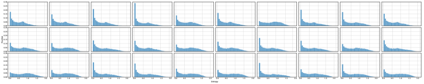
Figure 14: Softmax entropy histograms of 30 Wide-ResNet-28-10+SN models trained on CIFAR-10, evaluated on SVHN (OoD). The softmax entropy distribution of the different models varies considerably.

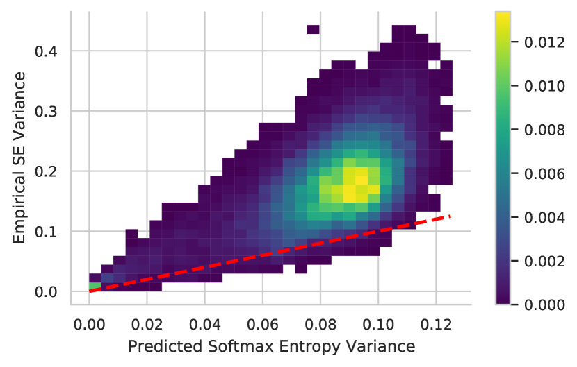
(a) Simulated vs Ground-Truth

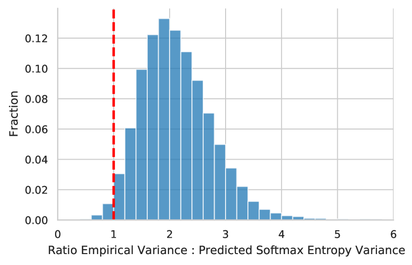
(b) Ratio Histogram

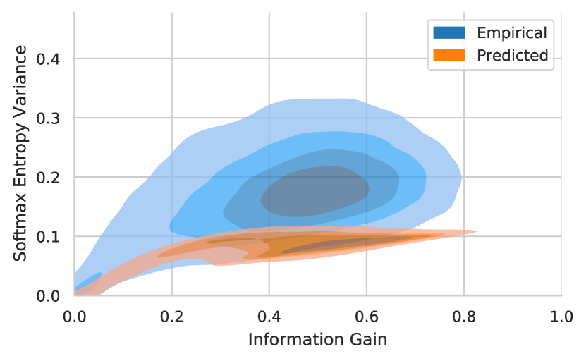
(c) Density Plot

Figure 15: The variance of softmax entropies can be lower-bounded by fitting Dirichlet distributions on the samples $\operatorname{p}(y\mathbin{|}x,\omega)$. 15(a) The empirical variance of softmax entropies is lower-bounded by $\operatorname{Var}[\operatorname{\mathbb{H}}[Y\mathbin{|}\mathbf{p}]]$. The red dashed line depicts equality. 15(b) The ratio histogram shows that there are only few violations due to precision issues ($<2\%$).15(c) The variance of the softmax entropy is not linearly correlated to the epistemic uncertainty. For both high and low epistemic uncertainty, the variance decreases.

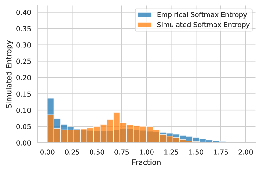
(a) WideResNet-28-10+SN

(b) VGG16

Figure 16: Simulated vs empirical softmax entropy on WideResNet-28-10+SN and VGG16. Even though the Dirichlet variance approximation lower-bounds the empirical softmax entropy variance, sampling from the fitted Dirichlet distributions does approximate the empirical entropy distribution quite well.

We empirically verify that softmax entropies vary considerably in Figure 14. In Figure 15, we verify that the predicted softmax entropy variance indeed lower-bounds the empirical softmax entropy variance. Morever, Figure 15(c) shows both i) the non-linear relationship between epistemic uncertainty and variance in the softmax entropies and ii) that Dirichlet distributions cannot capture it and can only provide a lower bound. Nonetheless, this simple approximation seems to be able to capture the empirical entropy distribution quite well as shown in Figure 16.

G.2 Objective Mismatch

In §5, we noted that the objectives that lead to optimal estimators for aleatoric and epistemic uncertainty via softmax entropy and feature-space density do not match, and DDU therefore uses the softmax layer as a discriminative classifier (implicit LDA) to estimate the predictive entropy, while it is using a GMM as generative classifier to estimate the feature-space density. Here we prove this.

G.2.1 Preliminaries

Before we prove Proposition 5.3, we will introduce some additional notation following Kirsch et al. (2020).

Definition G.7.

1. $\operatorname{\hat{p}}(y,z)$ is the data distribution of the $\mathcal{D}$ in feature space with class labels $y$ and feature representation $z$.

2. $\operatorname{p_{\theta}}(\cdot)$ is a probability distribution parameterized by $\theta$.

3. Entropies and conditional entropies are over the empirical data distribution $\operatorname{\hat{p}}(\cdot)$:

   $$\operatorname{\mathbb{H}}[\cdot]=\operatorname{\mathbb{H}}\left(\operatorname{\hat{p}}(\cdot)\right)=\operatorname{\mathbb{E}}_{\operatorname{\hat{p}}(\cdot)}\left[-\log\operatorname{\hat{p}}(\cdot)\right].$$ (46)

4. $\operatorname{\mathbb{H}}[Y\mathbin{|}z]$ is the entropy of $\operatorname{\hat{p}}(y\mathbin{|}z)$ for a given $z$, whereas $\operatorname{\mathbb{H}}[Y\mathbin{|}Z]$ is the conditional entropy:

   $$\operatorname{\mathbb{H}}[Y\mathbin{|}Z]=\operatorname{\mathbb{E}}_{\operatorname{\hat{p}}(z)}{\operatorname{\mathbb{H}}[Y\mathbin{|}z]}.$$ (47)

5. $\operatorname{\mathbb{H}}(\operatorname{p}(y,z)\mathbin{||}\operatorname{q}(y|z\mathbin{|}))$ is the cross-entropy of $\operatorname{q}(y\mathbin{|}z)$ under $\operatorname{p}(y\mathbin{|}z)$ in expectation over $\operatorname{p}(z)$:

   $$\operatorname{\mathbb{H}}(\operatorname{p}(y,z)\mathbin{||}\operatorname{q}(y\mathbin{|}z)) =\operatorname{\mathbb{E}}_{\operatorname{p}(z)}{\operatorname{\mathbb{H}}(\operatorname{p}(y\mathbin{|}z)\mathbin{||}\operatorname{q}(y\mathbin{|}z))}$$

   $$=\operatorname{\mathbb{E}}_{\operatorname{p}(y,z)}\left[-\log\operatorname{q}(y\mathbin{|}z)\right].$$

6. Similarly, $D_{\mathrm{KL}}(\operatorname{p}(y,z)\mathbin{||}\operatorname{q}(y|z\mathbin{|}))$ is the Kullback-Leibler divergence of $\operatorname{q}(y\mathbin{|}z)$ under $\operatorname{p}(y\mathbin{|}z)$ in expectation over $\operatorname{p}(z)$:

   $$D_{\mathrm{KL}}(\operatorname{p}(y,z)\mathbin{||}\operatorname{q}(y|z\mathbin{|})) =\operatorname{\mathbb{E}}_{\operatorname{p}(z)}{D_{\mathrm{KL}}(\operatorname{p}(y\mathbin{|}z)\mathbin{||}\operatorname{q}(y|z\mathbin{|}))}$$

   $$=\operatorname{\mathbb{H}}(\operatorname{p}(y,z)\mathbin{||}\operatorname{q}(y|z\mathbin{|}))-\operatorname{\mathbb{H}}[Y\mathbin{|}Z]$$

7. For cross-entropies of $\operatorname{p_{\theta}}(\cdot)$ under $\operatorname{\hat{p}}(z,y)$, we use the convenient short-hand $\operatorname{\mathbb{H}_{\theta}}[\cdot]=\operatorname{\mathbb{H}}(\operatorname{\hat{p}}(z,y)\mathbin{||}\operatorname{p_{\theta}}(\cdot))$.

Then we can observe the following connection between $\operatorname{\mathbb{H}_{\theta}}[\cdot]$ and $\operatorname{\mathbb{H}}[\cdot]$:

Lemma G.8.

Cross-entropies upper-bound the respective entropy with equality when $\operatorname{p_{\theta}}(\cdot)=\operatorname{\hat{p}}(\cdot)$, which is important for variational arguments:

1. $\operatorname{\mathbb{H}_{\theta}}[Y,Z]\geq\operatorname{\mathbb{H}}[Y,Z]$,

2. $\operatorname{\mathbb{H}_{\theta}}[Z]\geq\operatorname{\mathbb{H}}[Z]$, and

3. $\operatorname{\mathbb{H}_{\theta}}[Y\mathbin{|}Z]\geq\operatorname{\mathbb{H}}[Y\mathbin{|}Z]$.

Proof.

1. $\operatorname{\mathbb{H}_{\theta}}[Y,Z]-\operatorname{\mathbb{H}}[Y,Z]=D_{\mathrm{KL}}(\operatorname{\hat{p}}(y,z)\mathbin{||}\operatorname{p_{\theta}}(y,z))\geq 0.$

2. follows from Item 1.

3. We expand the expectations and note that inequality commutes with expectations:

   $$\operatorname{\mathbb{H}_{\theta}}[Y\mathbin{|}Z]-\operatorname{\mathbb{H}}[Y\mathbin{|}Z]=\operatorname{\mathbb{E}}_{\operatorname{\hat{p}}(z)}\left[\operatorname{\mathbb{H}_{\theta}}[Y\mathbin{|}z]-\operatorname{\mathbb{H}}[Y\mathbin{|}z]\right]\geq 0,$$

   because $\operatorname{\mathbb{H}_{\theta}}[Y\mathbin{|}z]-\operatorname{\mathbb{H}}[Y\mathbin{|}z]\geq 0$ for all $z$. The equality conditions follows from the properties of the Kullback-Leibler divergence as well.

∎

We also have:

Lemma G.9.

$$\operatorname{\mathbb{H}_{\theta}}[Y,Z] =\operatorname{\mathbb{H}_{\theta}}[Y\mathbin{|}Z]+\operatorname{\mathbb{H}_{\theta}}[Z]$$ (48)

$$=\operatorname{\mathbb{H}_{\theta}}[Z\mathbin{|}Y]+\operatorname{\mathbb{H}_{\theta}}[Y].$$ (49)

Proof.

We substitute the definitions and obtain:

$$\operatorname{\mathbb{H}_{\theta}}[Y,Z] =\operatorname{\mathbb{E}}_{\operatorname{p}(y,z)}\left[-\log\operatorname{q}(y,z)\right]$$ (50)

$$=\operatorname{\mathbb{E}}_{\operatorname{p}(y,z)}\left[-\log\operatorname{q}(y\mathbin{|}z)\right]+\operatorname{\mathbb{E}}_{\operatorname{p}(y,z)}\left[-\log\operatorname{q}(z)\right]$$ (51)

$$=\operatorname{\mathbb{H}_{\theta}}[Y\mathbin{|}Z]+\operatorname{\mathbb{H}_{\theta}}[Z].$$ (52)

∎

The same holds for entropies: $\operatorname{\mathbb{H}}[Y,Z]=\operatorname{\mathbb{H}}[Y\mathbin{|}Z]+\operatorname{\mathbb{H}}[Z]=\operatorname{\mathbb{H}}[Y\mathbin{|}Z]+\operatorname{\mathbb{H}}[Y]$ (Cover, 1999).

G.2.2 Proof

We can now prove the observation. See 5.3

Proof.

1. The conditional log-likelihood is a strictly proper scoring rule (Gneiting & Raftery, 2007). The optimization objective can be rewritten as

   $$\max_{\theta}\operatorname{\mathbb{E}}_{\log\operatorname{p_{\theta}}(y\mathbin{|}z)}{=}\min_{\theta}\operatorname{\mathbb{H}_{\theta}}[Y\mathbin{|}Z]\geq\operatorname{\mathbb{H}}[Y\mathbin{|}Z].$$ (53)

   An optimal discriminative classifier $\operatorname{p_{\theta}}(y\mathbin{|}z)$ would thus capture the true (empirical) distribution everywhere: $\operatorname{p_{\theta}}(y\mathbin{|}z)=\operatorname{\hat{p}}(y\mathbin{|}z)$. This means the negative conditional log-likelihood will be equal $\operatorname{\mathbb{H}}[Y\mathbin{|}Z]$ and $\operatorname{\mathbb{H}_{\theta}}[Y\mathbin{|}z]=\operatorname{\mathbb{H}}[Y\mathbin{|}z]$ for all $z$.

2. For density estimation $\operatorname{q}(z)$, the maximum likelihood $\operatorname{\mathbb{E}}\left[\log\operatorname{q}(z)\right]$ using the empirical data distribution is maximized. We can rewrite this as

   $$\max_{\theta}\operatorname{\mathbb{E}}_{\operatorname{\hat{p}}(y,z)}{\log\operatorname{p_{\theta}}(z)}=\min_{\theta}\operatorname{\mathbb{H}_{\theta}}[Z]\geq\operatorname{\mathbb{H}}[Z].$$ (54)

   We see that the negative marginalized likelihood of the density estimator upper-bounds the entropy of the feature representations $\operatorname{\mathbb{H}}[Z]$. We have equality and $\operatorname{p_{\theta}}(z)=\operatorname{\hat{p}}(z)$ in the optimum case.

3. Using $\operatorname{\mathbb{H}_{\theta}}[Y,Z]=\operatorname{\mathbb{H}_{\theta}}[Y\mathbin{|}Z]+\operatorname{\mathbb{H}_{\theta}}[Z]$, we can relate the objectives from Equation 53 and (54) to each other. First, we characterize a shared optimum, and then we show that both objectives are generally not minimized at the same time. For both objectives to be minimized, we have $\nabla\operatorname{\mathbb{H}_{\theta}}[Y\mathbin{|}Z]=0$ and $\nabla\operatorname{\mathbb{H}_{\theta}}[Z]=0$, and we obtain

   $$\nabla\operatorname{\mathbb{H}_{\theta}}[Y,Z]=\nabla\operatorname{\mathbb{H}_{\theta}}[Y\mathbin{|}Z]+\nabla\operatorname{\mathbb{H}_{\theta}}[Z]=0.$$ (55)

   From this we conclude that minimizing both objectives also minimizes $\operatorname{\mathbb{H}_{\theta}}[Y,Z]$, and that generally the objectives trade-off with each other at stationary points $\theta$ of $\operatorname{\mathbb{H}_{\theta}}[Y,Z]$:

   $$\nabla\operatorname{\mathbb{H}_{\theta}}[Y\mathbin{|}Z]=-\nabla\operatorname{\mathbb{H}_{\theta}}[Z]\quad\text{when $\nabla\operatorname{\mathbb{H}_{\theta}}[Y,Z]=0$}.$$ (56)

   This tells us that to construct a case where the optima do not coincide, discriminative classification needs to be opposed better density estimation.

   Specifially, when we have a GMM with one component per class, minimizing $\operatorname{\mathbb{H}_{\theta}}[Y,Z]$ on an empirical data distribution is equivalent to Gaussian Discriminant Analysis, as is easy to check, and minimizing $\operatorname{\mathbb{H}_{\theta}}[Z]$ is equivalent to fitting a density estimator, following Equation 54. The difference is that using a GMM as a density estimator does not constrain the component assignment, unlike in GDA.

   Consequently, we see that both objectives can be minimized at the same time exactly when the feature representations of different classes are perfectly separated, such that a GMM fit as density estimator would assign each class’s feature representations to a single component.

   By the above, we can construct a simple case: if the samples of different classes are not separated in feature-space, optimas for the objectives will not coincide, so for example if samples were drawn from the same Gaussian and labeled randomly. On the other hand, if we have classes whose features lie in well-separated clusters, GDA will minimize all objectives.

∎

Given that perfect separation is impossible with ambiguous data for a GMM, a shared optimum will be rare with noisy real-world data, but only then would GDA be optimal. In all other cases, GDA does not optimize both objectives, and neither can any other GMM with one component per class. Moreover, Equation 56 shows that a GMM fit using EM is a better density estimator than GDA, and a softmax layer is a better classifier, as optimizing the softmax objective $\operatorname{\mathbb{H}_{\theta}}[Y\mathbin{|}Z]$ or density objective $\operatorname{\mathbb{H}}[Z]$ using gradient descent will move away from the GDA optimum.

As can easily be verified, a trivial optimal minimizer $\operatorname{q}^{*}(y,z)$ for $\operatorname{\mathbb{H}_{\theta}}[Y,Z]$ given an empirical data distribution $\operatorname{\hat{p}}(y,z)$ is an adapted Parzen estimator:

$$\operatorname{q}^{*}(y,z)=\sum_{y}\operatorname{\hat{p}}(y)\operatorname{\mathbb{E}}_{\hat{z}\sim\operatorname{\hat{p}}(z\mathbin{|}y)}{\mathcal{N}(z;\,\hat{z},\,\sigma^{2}\mathbf{I})},$$ (57)

for small enough $\sigma$. This shows that above proposition is not general.

G.2.3 Intuitions & Validation with a Toy Example

Table 12: Realized objective scores (columns) for different optimization objectives (rows) for the synthetic 2D toy example depicted in Figure 6. Smaller is better. We see that each objectives minimizes its own score while being suboptimal in regards to the other two objectives (when it is possible to compute the scores). This empirically further validates Proposition 5.3.

Objective	$\operatorname{\mathbb{H}_{\theta}}[Y\mathbin{|}Z]$ ($\downarrow$)	$\operatorname{\mathbb{H}_{\theta}}[Y,Z]$ ($\downarrow$)	$\operatorname{\mathbb{H}_{\theta}}[Z]$ ($\downarrow$)
$\min\operatorname{\mathbb{H}_{\theta}}[Y\mathbin{|}Z]$	0.1794	5.4924	5.2995
$\min\operatorname{\mathbb{H}_{\theta}}[Y,Z]$	0.2165	4.9744	4.7580
$\min\operatorname{\mathbb{H}_{\theta}}[Z]$	n/a	n/a	4.7073

Figure 6 visualises this on a synthetic 2D dataset with three classes and 4% label noise, which causes the optima to diverge as described in the proof. Label noise is a common issue in real-world datasets. Non-separability even more so. To explain Proposition 5.3 in an intuitive way, we focus on on a simple 2D toy case and fit a GMM using the different objectives. We sample "latents" z from 3 Gaussians (each representing a different class y) with 4% label noise. Following the construction in the proof, this will lead the objectives to have different optima.

We know discuss the different objectives in Figure 6 and the resulting scores in more detail:

${\min\operatorname{\mathbb{H}_{\theta}}[Y\mathbin{|}Z]}$. A softmax linear layer is equivalent to an LDA (Linear Discriminant Analysis) with conditional likelihood as detailed in Murphy (2012), for example. We optimize an LDA with the usual objective "$\min-1/N\sum\log\operatorname{p}(y\mathbin{|}z)$", i.e. the cross-entropy of $\operatorname{p}(y\mathbin{|}z)$ or (average) negative log-likelihood (NLL). Following Definition G.7, we use the short-hand "$\min\operatorname{\mathbb{H}_{\theta}}[Y\mathbin{|}Z]$" for this cross-entropy.

Because we optimize only $\operatorname{p}(y\mathbin{|}z)$, $\operatorname{p}(z)$ does not affect the objective and is thus not optimized. Indeed, the components do not actually cover the latents well, as can be seen in the first density plot of Figure 6(a). However, it does provide the lowest NLL.

$\min\operatorname{\mathbb{H}_{\theta}}[Y,Z]$. We optimize a GDA for the combined objective "$\min-1/N\sum\log\operatorname{q}(y,z)$", i.e. the cross-entropy of $\operatorname{q}(y,z)$. We use the short-hand "$\min\operatorname{\mathbb{H}_{\theta}}[Y\mathbin{|}Z]$" for this.

$\min\operatorname{\mathbb{H}_{\theta}}[Z]$. We optimize a GMM for the objective "$\min-1/N\sum\log\operatorname{q}(z)$", i.e. the cross-entropy of $\operatorname{q}(z)$. We use the short-hand "$\min\operatorname{\mathbb{H}_{\theta}}[Z]$" for this.

We do not provide scores for $\operatorname{\mathbb{H}_{\theta}}[Y\mathbin{|}Z]$ and $\operatorname{\mathbb{H}_{\theta}}[Y,Z]$ for the third objective $\min\operatorname{\mathbb{H}_{\theta}}[Z]$ in Table 12 as it does not depend on $Y$, and hence the different components do not actually model the different classes necessarily. Hence, we also use a single color to visualize the components for this objective in Figure 6(a).

In Table 12 and Figure 6(a), we see that each solution minimizes its own objective best. The GMM provides the best density model (best fit according to the entropy), while the LDA (like a softmax linear layer) provides the best NLL for the labels. The GDA provides a density model that is almost as good.

Entropy. Looking at the entropy plots in Figure 6(b), we first notice that the LDA solution optimized for $\min\operatorname{\mathbb{H}_{\theta}}[Y\mathbin{|}Z]$ has a wide decision boundary. This is due to the overlap of the Gaussian components, which is necessary to provide the right aleatoric uncertainty.

Optimizing the negative log-likehood $-\log\operatorname{p}(y\mathbin{|}z)$ is a proper scoring rule, and hence is optimized for calibrated predictions.

Compared to this, the GDA solution (optimized for $\min\operatorname{\mathbb{H}_{\theta}}[Y,Z]$ has a much narrower decision boundary and cannot capture aleatoric uncertainty as well. This is reflected in the higher NLL. Moreover, unlike for LDA, GDA decision boundaries behave differently than one would naively expect due to the untied covariance matrices. They can be curved and the decisions change far away from the data (Murphy, 2012).

To show the difference between the two objectives we have marked an ambiguous point near $(0,-5)$ with a yellow star . Under the first objective $\min\operatorname{\mathbb{H}_{\theta}}[Y,Z]$, the point has high aleatoric uncertainty (high entropy), as seen in the left entropy plot while under the second objective ($\min\operatorname{\mathbb{H}_{\theta}}[Y,Z]$) the point is only assigned very low entropy. The GDA optimized for the second objective thus is overconfident.

As above explained above, we do not show an entropy plot of $Y\mid Z$ for the third objective $\min\operatorname{\mathbb{H}_{\theta}}[Z]$ in Figure 6(b) because the objective does not depend on $Y$, and there are thus no class predictions.

Intuitively, for aleatoric uncertainty, the Gaussian components need to overlap to express high aleatoric uncertainty (uncertain labelling). At the same time, this necessarily provides looser density estimates. On the other hand, the GDA density is much tighter, but this comes at the cost of NLL for classification because it cannot express aleatoric uncertainty that well. Figure 6 visualizes how the objectives trade-off between each other, and why we use the softmax layer trained for $\operatorname{p}(y\mathbin{|}z)$ for classification and aleatoric uncertainty, and GDA as density model for $\operatorname{q}(z)$.

(a) Dirty-MNIST (iD) and Fashion-MNIST (OoD)

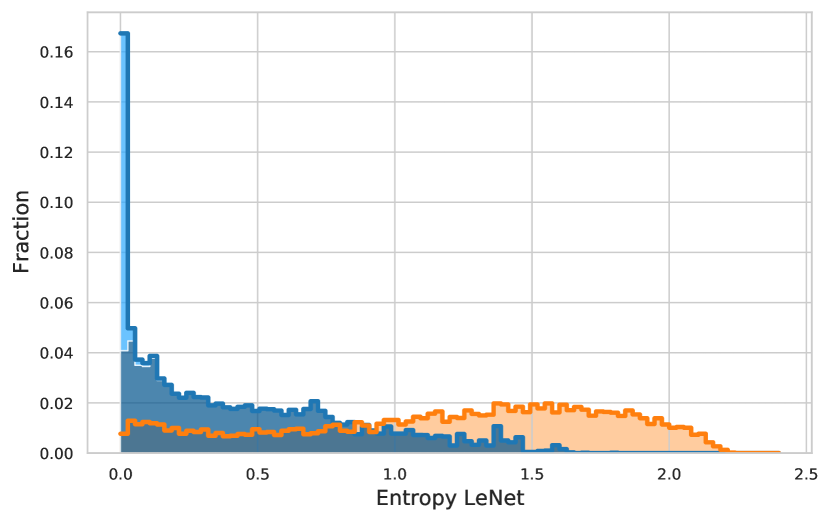
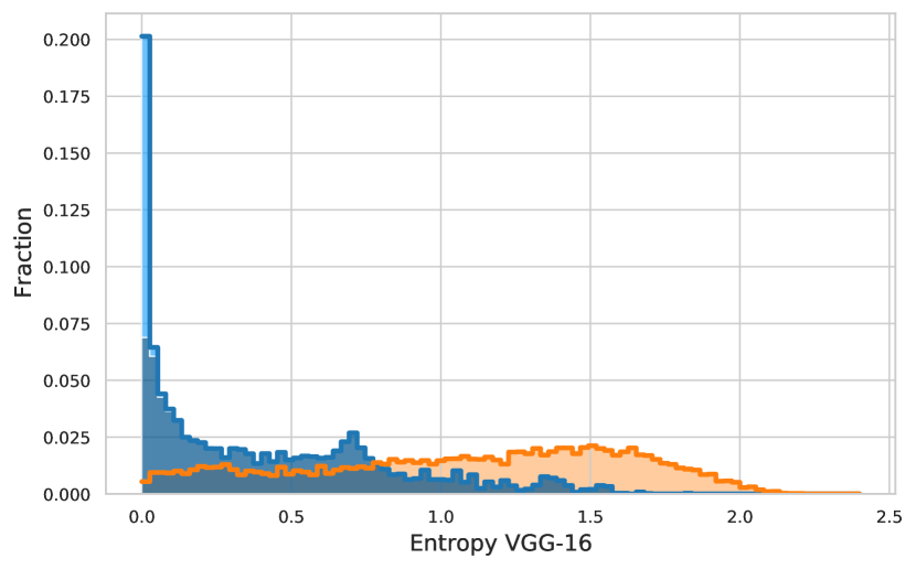
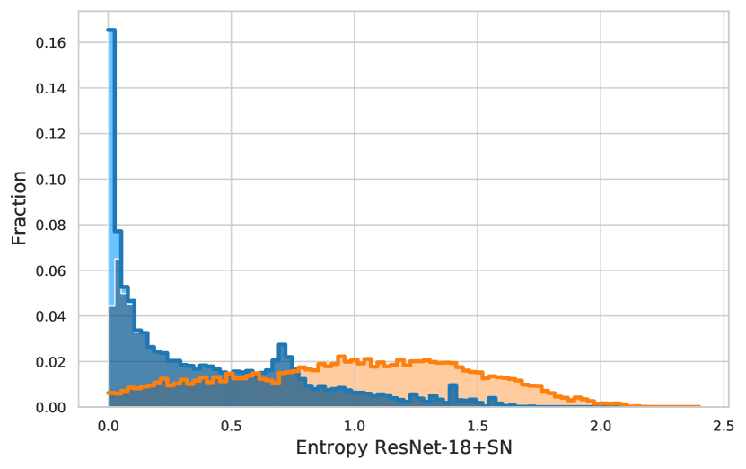
(b) Softmax entropy

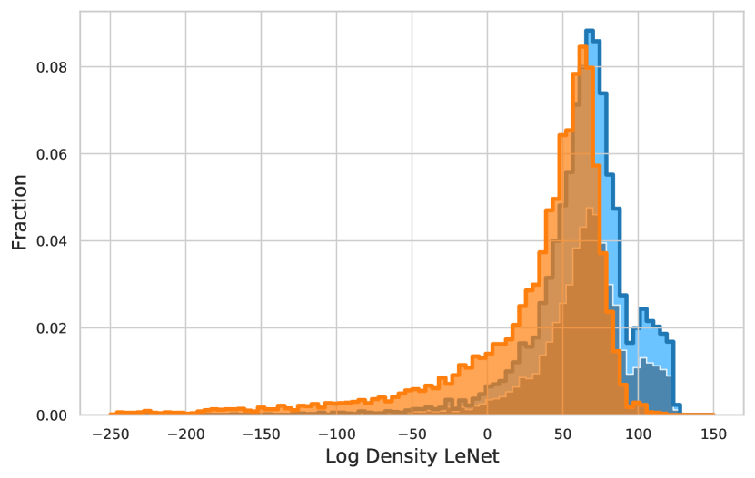
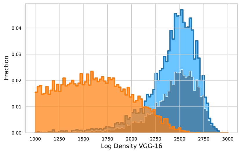
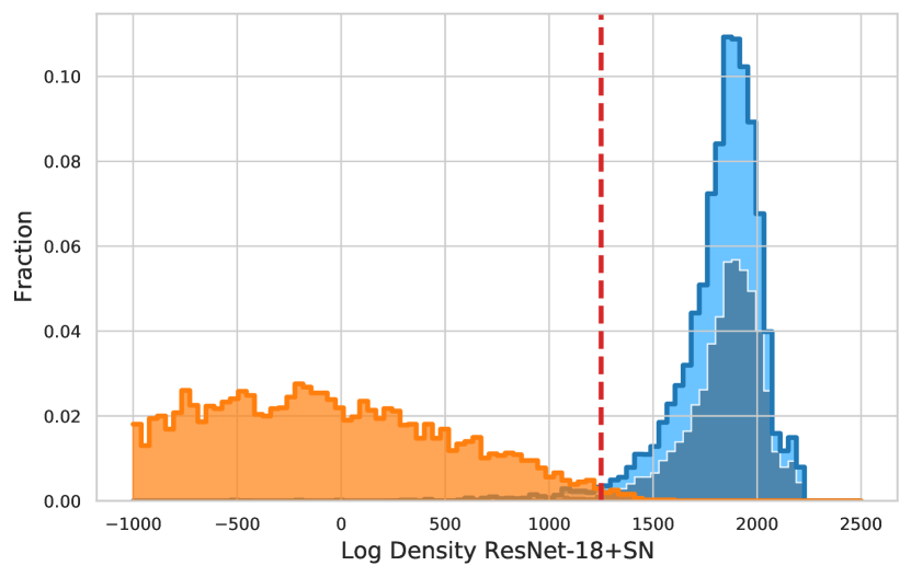
(c) Feature-space density

Figure 17: Disentangling aleatoric and epistemic uncertainty on Dirty-MNIST (iD) and Fashion-MNIST (OoD) 17(a) requires using softmax entropy 17(b) and feature-space density (GMM) 17(c) with appropriate inductive biases (ResNet-18+SN vs LeNet & VGG-16 without them). Enlarged version. 17(b): Softmax entropy captures aleatoric uncertainty for iD data (Dirty-MNIST), thereby separating unambiguous MNIST samples and Ambiguous-MNIST samples. However, iD and OoD are confounded: softmax entropy has arbitrary values for OoD, indistinguishable from iD. 17(c): With appropriate inductive biases (DDU with ResNet-18+SN), iD and OoD densities do not overlap, capturing epistemic uncertainty. However, without appropriate inductive biases (LeNet & VGG-16), feature density suffers from feature collapse: iD and OoD densities overlap. Generally, feature-space density confounds unambiguous and ambiguous iD samples as their densities overlap. Note: Unambiguous MNIST samples and Ambiguous-MNIST samples are shown as stacked histograms with the total fractions adding up to 1 for Dirty-MNIST.

References

- Blundell et al. (2015) Blundell, C., Cornebise, J., Kavukcuoglu, K., and Wierstra, D. Weight uncertainty in neural network. In International Conference on Machine Learning, pp. 1613–1622. PMLR, 2015.
- Buitinck et al. (2013) Buitinck, L., Louppe, G., Blondel, M., Pedregosa, F., Mueller, A., Grisel, O., Niculae, V., Prettenhofer, P., Gramfort, A., Grobler, J., Layton, R., VanderPlas, J., Joly, A., Holt, B., and Varoquaux, G. API design for machine learning software: experiences from the scikit-learn project. In ECML PKDD Workshop: Languages for Data Mining and Machine Learning, pp. 108–122, 2013.
- Cohn et al. (1996) Cohn, D. A., Ghahramani, Z., and Jordan, M. I. Active learning with statistical models. Journal of artificial intelligence research, 4:129–145, 1996.
- Cover (1999) Cover, T. M. Elements of information theory. John Wiley & Sons, 1999.
- Deng et al. (2009) Deng, J., Dong, W., Socher, R., Li, L.-J., Li, K., and Fei-Fei, L. Imagenet: A large-scale hierarchical image database. In 2009 IEEE conference on computer vision and pattern recognition, pp. 248–255. Ieee, 2009.
- Der Kiureghian & Ditlevsen (2009) Der Kiureghian, A. and Ditlevsen, O. Aleatory or epistemic? does it matter? Structural safety, 31(2):105–112, 2009.
- DeVries & Taylor (2018) DeVries, T. and Taylor, G. W. Learning confidence for out-of-distribution detection in neural networks. arXiv preprint arXiv:1802.04865, 2018.
- Dinh et al. (2015) Dinh, L., Krueger, D., and Bengio, Y. Nice: Non-linear independent components estimation, 2015.
- Dusenberry et al. (2020) Dusenberry, M., Jerfel, G., Wen, Y., Ma, Y., Snoek, J., Heller, K., Lakshminarayanan, B., and Tran, D. Efficient and scalable bayesian neural nets with rank-1 factors. In International conference on machine learning, pp. 2782–2792. PMLR, 2020.
- Esteva et al. (2017) Esteva, A., Kuprel, B., Novoa, R. A., Ko, J., Swetter, S. M., Blau, H. M., and Thrun, S. Dermatologist-level classification of skin cancer with deep neural networks. nature, 542(7639):115–118, 2017.
- Filos et al. (2019) Filos, A., Farquhar, S., Gomez, A. N., Rudner, T. G., Kenton, Z., Smith, L., Alizadeh, M., de Kroon, A., and Gal, Y. A systematic comparison of bayesian deep learning robustness in diabetic retinopathy tasks. arXiv preprint arXiv:1912.10481, 2019.
- Gal (2016) Gal, Y. Uncertainty in Deep Learning. PhD thesis, University of Cambridge, 2016.
- Gal & Ghahramani (2016) Gal, Y. and Ghahramani, Z. Dropout as a bayesian approximation: Representing model uncertainty in deep learning. In international conference on machine learning, pp. 1050–1059, 2016.
- Gal et al. (2017) Gal, Y., Islam, R., and Ghahramani, Z. Deep bayesian active learning with image data. In International Conference on Machine Learning, pp. 1183–1192. PMLR, 2017.
- Gneiting & Raftery (2007) Gneiting, T. and Raftery, A. E. Strictly proper scoring rules, prediction, and estimation. Journal of the American statistical Association, 102(477):359–378, 2007.
- Gouk et al. (2021) Gouk, H., Frank, E., Pfahringer, B., and Cree, M. J. Regularisation of neural networks by enforcing lipschitz continuity. Machine Learning, 110(2):393–416, 2021.
- Gulrajani et al. (2017) Gulrajani, I., Ahmed, F., Arjovsky, M., Dumoulin, V., and Courville, A. C. Improved training of wasserstein gans. In NeurIPS, 2017.
- Guo et al. (2017) Guo, C., Pleiss, G., Sun, Y., and Weinberger, K. Q. On calibration of modern neural networks. arXiv preprint arXiv:1706.04599, 2017.
- He et al. (2020) He, B., Lakshminarayanan, B., and Teh, Y. W. Bayesian Deep Ensembles via the Neural Tangent Kernel. In Advances in neural information processing systems, 2020.
- He et al. (2016) He, K., Zhang, X., Ren, S., and Sun, J. Deep residual learning for image recognition. In Proceedings of the IEEE conference on computer vision and pattern recognition, pp. 770–778, 2016.
- Hendrycks & Dietterich (2019) Hendrycks, D. and Dietterich, T. Benchmarking neural network robustness to common corruptions and perturbations. arXiv preprint arXiv:1903.12261, 2019.
- Hendrycks & Gimpel (2016) Hendrycks, D. and Gimpel, K. A baseline for detecting misclassified and out-of-distribution examples in neural networks. arXiv preprint arXiv:1610.02136, 2016.
- Hendrycks et al. (2018) Hendrycks, D., Mazeika, M., and Dietterich, T. Deep anomaly detection with outlier exposure. In International Conference on Learning Representations, 2018.
- Hendrycks et al. (2021) Hendrycks, D., Zhao, K., Basart, S., Steinhardt, J., and Song, D. Natural adversarial examples. In Proceedings of the IEEE/CVF Conference on Computer Vision and Pattern Recognition, pp. 15262–15271, 2021.
- Hernández-Lobato & Adams (2015) Hernández-Lobato, J. M. and Adams, R. Probabilistic backpropagation for scalable learning of bayesian neural networks. In International Conference on Machine Learning, pp. 1861–1869. PMLR, 2015.
- Hinton & Van Camp (1993) Hinton, G. E. and Van Camp, D. Keeping the neural networks simple by minimizing the description length of the weights. In Proceedings of the sixth annual conference on Computational learning theory, pp. 5–13, 1993.
- Hsu et al. (2020) Hsu, Y.-C., Shen, Y., Jin, H., and Kira, Z. Generalized odin: Detecting out-of-distribution image without learning from out-of-distribution data. In CVPR, 2020.
- Huang et al. (2017) Huang, G., Liu, Z., Van Der Maaten, L., and Weinberger, K. Q. Densely connected convolutional networks. In Proceedings of the IEEE conference on computer vision and pattern recognition, pp. 4700–4708, 2017.
- Huang & Chen (2020) Huang, Y. and Chen, Y. Autonomous driving with deep learning: A survey of state-of-art technologies. arXiv preprint arXiv:2006.06091, 2020.
- Kendall & Gal (2017) Kendall, A. and Gal, Y. What uncertainties do we need in bayesian deep learning for computer vision? In Advances in neural information processing systems, pp. 5574–5584, 2017.
- Kingma & Ba (2015) Kingma, D. P. and Ba, J. Adam: A method for stochastic optimization. In ICLR, 2015.
- Kingma & Welling (2014) Kingma, D. P. and Welling, M. Auto-encoding variational bayes. In ICLR, 2014.
- Kirsch et al. (2019) Kirsch, A., van Amersfoort, J., and Gal, Y. Batchbald: Efficient and diverse batch acquisition for deep bayesian active learning. In Advances in Neural Information Processing Systems, 2019.
- Kirsch et al. (2020) Kirsch, A., Lyle, C., and Gal, Y. Unpacking information bottlenecks: Unifying information-theoretic objectives in deep learning. arXiv preprint arXiv:2003.12537, 2020.
- Kristiadi et al. (2020) Kristiadi, A., Hein, M., and Hennig, P. Being bayesian, even just a bit, fixes overconfidence in relu networks. In ICML, 2020.
- Krizhevsky et al. (2009) Krizhevsky, A., Hinton, G., et al. Learning multiple layers of features from tiny images. 2009.