Quasi-Distributed Antenna Selection for Spectral Efficiency Maximization in Subarray Switching XL-MIMO Systems

Abstract

In this paper, we consider the downlink (DL) of a zero-forcing (ZF) precoded extra-large scale massive MIMO (XL-MIMO) system. The base-station (BS) operates with limited number of radio-frequency (RF) transceivers due to high cost, power consumption and interconnection bandwidth associated to the fully digital implementation. The BS, which is implemented with a subarray switching architecture, selects groups of active antennas inside each subarray to transmit the DL signal. This work proposes efficient resource allocation (RA) procedures to perform joint antenna selection (AS) and power allocation (PA) to maximize the DL spectral efficiency (SE) of an XL-MIMO system operating under different loading settings. Two metaheuristic RA procedures based on the genetic algorithm (GA) are assessed and compared in terms of performance, coordination data size and computational complexity. One algorithm is based on a quasi-distributed methodology while the other is based on the conventional centralized processing. Numerical results demonstrate that the quasi-distributed GA-based procedure results in a suitable trade-off between performance, complexity and exchanged coordination data. At the same time, it outperforms the centralized procedures with appropriate system operation settings.

I Introduction

The benefits of adopting a high number of antennas at the base-station (BS) have attracted the interest on the massive MIMO transceiver design for the multi-antenna wireless communications systems beyond the fifth generation (B5G) and of the sixth generation (6G). The main advantages are the large array gain, inter-channel orthogonality and channel hardening. Also, increasing the number of antenna elements can enhance the cell coverage, improving the quality-of-service (QoS) of the border-cell users [1].

When the BS array attains extreme physical dimensions to support crowded scenario locations, such as airports and large shopping malls, the system is classified as extra-large scale massive MIMO (XL-MIMO) [2]. The XL-MIMO array provides the benefits of massive MIMO with additional beam-forming resolution due to the large array aperture [3]. The XL-MIMO array is characterized by key changes in the electromagnetic propagation conditions when compared to the conventional spatial stationary massive MIMO regime. The first property is the spherical wavefront propagation feature for the received signal due to the distance between the BS and the users being less than the Rayleigh distance [4]. Second, each cluster of scatterers sees only a portion of the array. Thus, the transmitted signal by each user reaches a small group of antennas, which comprises the visibility region (VR) of this user [2]. Additionally, the different propagation paths experienced along the array result in variations on the average received power. Results in [5, 6] demonstrate that the spatial non-stationarities produced by these two properties limit the performance of the system in terms of spectral efficiency (SE) unless an appropriated signal processing technique is applied.

Despite the benefits of high numbers of antennas, the XL-MIMO scenario imposes challenges for transceiver design. The first of them is the high cost and power consumption of fully digital implementations, which require one radio-frequency (RF) transceiver per antenna element [7, 8]. In addition, adopting a large number of antennas demands a high interconnection bandwidth to transmit the baseband data throughout the links to the BS processing unit. This turns into a serious implementation bottleneck, since the required bandwidth can not be handled by the current radio interfaces [9, 10]. Lastly, handling the complexity of signal processing techniques is a relevant issue, since the number of executed operations in linear detectors, such as zero-forcing (ZF) and minimum mean-squared error (MMSE), scales with the number of antennas [11].

In order to design practical BS architectures, one can limit the number of RF transceivers to cope with the cost constraints. The implementation with a limited the number of RF transceivers can benefit from the large array by adopting techniques such as antenna selection (AS) and hybrid precoding. Often, hybrid precoding design is associated with the solution of intricate optimization problems [12]. In addition, the commonly employed analog phase shifters are more expensive and consume more power than conventional on-off switches [8]. For these reasons, combining the AS procedures with linear precoding designs result in attainable strategies aiming at robust and effective implementations. Different approaches and tools can be adopted to perform AS, such as convex optimization [13, 14, 7], greedy heuristics [7, 15], machine learning [16] and metaheuristics [17, 18, 19, 20].

One strategy to combat the problem of high interconnection bandwidth is to use hierarchical architectures. Adding multiple processing units to handle small groups of antennas and choosing the right signal processing methods can reduce significantly the amount of exchanged information in the regime of asymptotic number of antennas, as discussed in [10, 9]. However, the coordination of such processing units to perform different signal processing and resource allocation (RA) tasks constitutes a big challenge. In addition, many of these activities rely on the knowledge of fully reliable channel state information (CSI), which is hard to attain due to the high array dimensions. Many works on channel estimation [21], precoding and data detection [22, 23, 24, 25, 10, 9] in massive and XL-MIMO consider distributed pre-processing at local nodes. However, studies on the distributed RA strategies, mainly involving AS, are scarce.

The signal processing complexity is an important concern in XL-MIMO due to the high number of antenna elements. However, differently from the conventional massive MIMO, the XL-MIMO can benefit from the spatial non-stationarities adopting local signal processing strategies to treat the signals inside the VRs at the BS’ sub-arrays with reduced complexity [22, 24].

I-A Literature Review

AS strategies for MIMO systems are extensively discussed in the literature. One AS algorithm to improve capacity in low rank matrix channels on point-to-point MIMO was first introduced in [26]. Later, the capacity distribution of systems with receive AS has been derived in [27]. These results were extended to massive MIMO regime in [28] and [29]. In these papers, the authors derived capacity bounds for systems with transmit and receive AS, respectively.

The authors in [13, 14] proposed AS procedures respectively for the channel capacity and downlink (DL) sum-capacity maximization based on the convex optimization framework. One technique based on the branch-and-bound algorithm is used in [8]. Considering linearly-precoded systems, the problems of AS for SE and sum-SINR maximization are addressed respectively in [15, 30]. Differently, the work in [31] analyzed one joint AS and power allocation (PA) procedure in a system with spatially distributed antennas. The proposed procedure runs at each antenna with side-information shared within its neighborhood. Besides, AS considering limited connections in the RF transceivers switching matrices is examined in [7].

On the other hand, there are only a few works that consider the AS problem for the XL-MIMO systems. A spatial users mapping procedure to maximize SE implemented with convolutional neural networks (CNN) is proposed in [16]. The aim is to determine each effective subarray window to precode the users signals using ZF. Results demonstrate that the CNN-based procedure achieves SE values comparable to the optimal mapping algorithm. In [17], several transmit AS procedures to maximize the energy efficiency (EE) from the long-term fading coefficients are proposed. Asymptotic SINR expressions for the received signal with AS are derived. Since the derived optimization problem is NP-hard, three of the proposed procedures are implemented by metaheuristic techniques, one being the genetic algorithm (GA). The GA is a powerful evolutionary metaheuristic that was used in different contexts to solve AS problems, as it is considered in [18, 19, 20].

I-B Contribution

Motivated by the benefits of large numbers of antennas at the BS and the restricted number of RF transceivers, this work examines the joint AS and PA problem on the DL of a linearly-precoded XL-MIMO system. Differently from other papers adopting AS strategy, a distributed BS signal processing architecture is considered and the AS procedures are characterized in terms of the exchanged information between the processing nodes. Furthermore, we extend part of the results of [17] with the proposition of AS algorithms for XL-MIMO that use the short-term fading coefficients instead of the long-term ones. Additionally, we address the problem of joint AS and PA in XL-MIMO sub-arrays using a decentralized RA algorithm. The proposed RA algorithm uses the Sherman-Morrison-Woodbury (SMW) formula to perform optimal power allocation (OPA) and AS in a decentralized fashion.

The BS is constituted by multiple non-overlapping subarrays with dedicated remote processing units (RPUs), which perform independently channel estimation, precoding calculation and RA, mainly AS and PA. Each subarray is equipped with a fixed number of antenna elements and RF transceivers. Using the ZF precoding, the optimization goal is to maximize the SE subjected to the constraints of subarrays connections and maximum transmitted power.

The contribution of this work is fourfold. i) Description of a distributed transceiver design for XL-MIMO based on a subarray switching architecture; ii) proposition of a centralized procedure based on the evolutionary heuristic GA to perform joint AS and PA to maximize the SE with subarray connection and maximum transmitted power constraints; iii) proposition of a distributed version of the GA procedure for joint AS and PA which achieves performance tight to the centralized one but with low-size coordination data and less number of executed operations; iv) extensive analyses of the proposed procedures in terms of number of symbols for training, coordination data size and number of floating point operations per second (flops).

The numerical results corroborate the GA-based procedures in achieving high performance, specifically in crowded XL-MIMO applications. Additionally, the decentralized GA version offers a good trade-off between performance, number of operations and coordination data size, outperforming the centralized procedures by adopting proper settings.

The rest of the paper is organized as follows. In Section II is described the system model, including the distributed subarrays processing at the BS. Next, in Section III are described the centralized and distributed GA-based optimization procedures for joint AS and PA in XL-MIMO systems, while Section IV discusses two feasible AS procedures adopted as a result of decoupling the joint AS and PA optimization problem. Section V examines the complexity of the proposed algorithms. Extensive numerical results are discussed in Section VI. Final comments and conclusions are provided in Section VII.

I-C Notation

Boldface small $\mathbf{a}$ and capital $\mathbf{A}$ letters represent respectively vectors and matrices. Capital calligraphic letters $\mathcal{A}$ represent finite sets, and $|\mathcal{A}|$ denotes the cardinality of the set $\mathcal{A}$. $\mathbf{I}_{n}$ denotes the identity matrix of size $n$. $\{\cdot\}^{T}$ and $\{\cdot\}^{H}$ denote respectively the transpose and the conjugate transpose operators. $\textrm{diag}(\cdot)$, $\textrm{tr}(\cdot)$ and $\textrm{det}(\cdot)$ denote respectively the diagonal matrix, trace and determinant operators. $\left\lceil\cdot\right\rceil$ denotes the greatest integer operator. $\binom{n}{k}$ denotes the binomial coefficient. $\mathcal{CN}(\mu,\sigma^{2})$ is a circularly symmetric complex Gaussian distribution with mean $\mu$ and variance $\sigma^{2}$. $\mathbb{E}[\cdot]$ denotes the expectation operator.

II System Model

Consider the DL of a narrow-band multi-user XL-MIMO system with the BS equipped with $M$ antennas and $N$ RF transceivers serving $K$ single-antenna users, as is depicted in Fig. 1. During the DL, the BS uses $\eta_{\rm tr}$ symbols to perform channel estimation and $\eta_{\rm data}$ symbols to transmit the payload. We assume that the time interval used to send the total DL symbols $\eta_{\textsc{dl}}=\eta_{\rm tr}+\eta_{\rm data}$ is less than the channel coherence time.

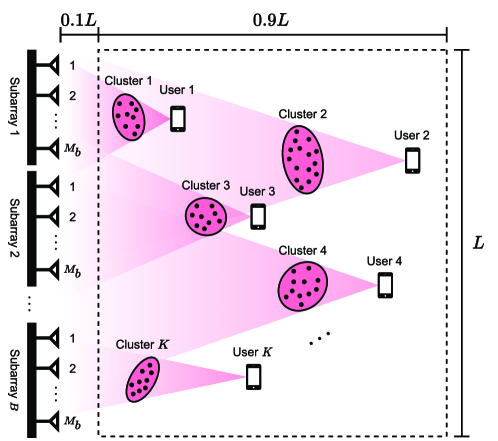
Figure 1: XL-MIMO system deployed inside a square cell with size $L$. The BS is a ULA with $M$ antennas divided into $B$ subarrays of $M_{b}$ antennas each one. The $K$ users are randomly distributed at a distance in the range $(0.1L,L)$ from the array.

The array in the BS is composed of $B$ independent subarrays, each with $M_{b}$ antennas and $N_{b}<M_{b}$ RF transceivers. The subarrays are equipped with a RPU to perform, in a distributed way, channel estimation, precoding calculation and RA tasks, specially AS and PA procedures. In addition, the BS has a central processing unit (CPU) to coordinate the subarrays operation. Fig. 2 depicts all the described BS blocks.

Assumption 1 (Subarray switching stage): A flexible switching stage is implemented in each XL subarray. This stage allows every antenna of the subarray $i$ to connect to any RF transceiver of it. Results in [7] demonstrate that partially connected architectures introduce lower insertion loss than fully-flexible matrices, which allows the connection of any antenna in the entire array to any RF transceiver.

We assume that each subarray has perfect knowledge of the channel coefficients associated to its antennas. See [21] for details on channel acquisition in distributed signal processing architectures. Besides, we deploy the ZF precoder to decode signals in each subarray. We adopt the technique in [21] to calculate the ZF precoder with low interconnection traffic, splitting the computations between the RPUs and the CPU.

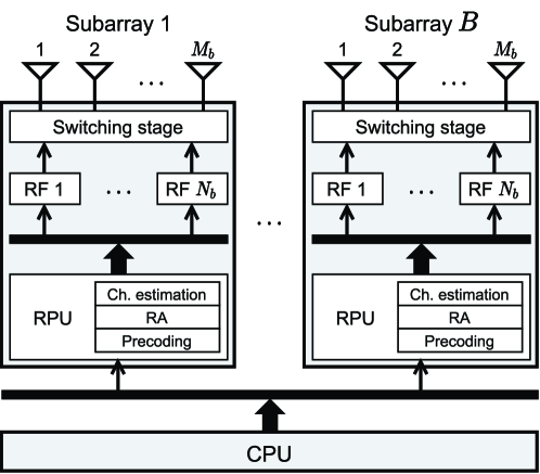
Figure 2: Diagram of the BS architecture for DL. The BS array is composed by $B$ subarrays containing $M_{b}$ antennas, $N_{b}$ RF transceivers and one RPU. Additionally, the BS has a CPU for subarrays coordination.

II-A Channel Model

In the XL-MIMO scenario, spatial non-stationarities arise due to the large array physical dimensions and number of antenna elements. Such non-stationarities are addressed in the adopted channel model as the variation of the mean received power along the array, as in [22, 17]. The path-loss coefficient associated to the BS antenna $m$ and the user $k$ is defined as

$$\beta_{m,k}=q_{0}d_{m,k}^{-\kappa}$$ (1)

where $q_{0}$ is the path-loss attenuation at a reference distance, $d_{m,k}$ is the distance between the antenna $m$ and the user $k$ and $\kappa$ is the path-loss exponent.

Let $\mathbf{R}_{k}\in\mathbb{C}^{M\times M}$, $\mathbf{R}_{k}=\textrm{diag}([\beta_{1,k}\;\cdots\;\beta_{M,k}]^{T})$ be the matrix with the long-term fading coefficients of the user $k$. The channel vector of the user $k$ is defined as

$$\mathbf{h}_{k}=\mathbf{R}_{k}^{\frac{1}{2}}\mathbf{h}_{k}^{\prime}$$ (2)

where $\mathbf{h}_{k}^{\prime}\in\mathbb{C}^{M\times 1}$, $\mathbf{h}_{k}^{\prime}\sim\mathcal{CN}\left(\mathbf{0},\mathbf{I}_{M}\right)$ is the short-term fading vector. From the users channel vectors, the channel matrix $\mathbf{H}\in\mathbb{C}^{M\times K}$ is defined as

$$\mathbf{H}=\begin{bmatrix}\mathbf{h}_{1}&\cdots&\mathbf{h}_{K}\end{bmatrix}=\begin{bmatrix}\mathbf{\underline{h}}_{1}^{T}&\cdots&\mathbf{\underline{h}}_{M}^{T}\end{bmatrix}^{T}$$ (3)

considering $\mathbf{\underline{h}}_{m}\in\mathbb{C}^{1\times K}$ as the channel vector with the coefficients associated to the antenna $m$.

During the DL, the BS activates a group of antennas represented by the set $\mathcal{S}\subseteq\left\{1,\dots,M\right\}$ such that $|\mathcal{S}|\leq N$. A partition of the set $\mathcal{S}$, i.e. $\{\mathcal{S}_{b}\}$, $\forall b=1,\dots,B$, contains the index of the selected antennas in the subarray $b$. This set is defined such that $|\mathcal{S}_{b}|\leq N_{b}\;\forall b$, meeting the adopted subarray structure. The equivalent channel matrix of the active antennas is defined as a row-wise submatrix of $\mathbf{H}$, $\mathbf{H}_{\mathcal{S}}{\in\mathbb{C}^{|\mathcal{S}|\times K}}$. Similarly, the matrix $\mathbf{H}_{\mathcal{S}_{b}}{\in\mathbb{C}^{|\mathcal{S}_{b}|\times K}}$ contains only the channel vectors related to the active antennas in the subarray $b$.

Let $D_{m}\in\left\{0,1\right\},\;\forall m=1,\dots,M$ be an indicator equal to 1 if the antenna $m$ is active during the DL and 0 otherwise. These indicators form the diagonal matrix $\mathbf{D}=\textrm{diag}([D_{1}\;\cdots\;D_{M}]^{T})$. During the precoding and SE computations, it is required to calculate the matrix product $\mathbf{H}_{\mathcal{S}}^{H}\mathbf{H}_{\mathcal{S}}$ of the active antennas channel matrix. Intended to enable this computation by the distributed signal processing architecture, the Gramian matrix is defined as in the following.

Remark 1 (Gramian matrix): Let $\mathbf{G}_{m}=\mathbf{\underline{h}}_{m}^{H}\mathbf{\underline{h}}_{m},\;\forall m=1,\dots,M$ be the Gramian matrix associated with the BS antenna $m$. The set $\mathcal{M}_{b}$ is defined for $b=1,\dots,B$ as the group of antennas in the subarray $b$. The Gramian matrix associated to the $b$-th subarray includes only the active antennas inside it, and it can be written as

$$\mathbf{G}_{\mathcal{S}_{b}}=\mathbf{H}_{\mathcal{S}_{b}}^{H}\mathbf{H}_{\mathcal{S}_{b}}=\sum_{m\in\mathcal{M}_{b}}D_{m}\mathbf{G}_{m}$$ (4)

Similarly, the array Gramian matrix considering only the active antennas is defined as

$$\mathbf{G}_{\mathcal{S}}=\mathbf{H}_{\mathcal{S}}^{H}\mathbf{H}_{\mathcal{S}}=\sum_{m=1}^{M}D_{m}\mathbf{G}_{m}$$ (5)

An upper bound for the system performance considering the active antennas in the set $\mathcal{S}$, namely the DL sum-capacity, is calculated by [14]:

$$C_{\textsc{dpc}} =\underset{\mathbf{P}}{\textrm{max}}\log_{2}\textrm{det}\left(\mathbf{I}_{K}+\frac{1}{\sigma_{z}^{2}}\mathbf{PH}_{\mathcal{S}}^{H}\mathbf{H}_{\mathcal{S}}\right)$$ (6)

$$=\underset{\mathbf{P}}{\textrm{max}}\log_{2}\textrm{det}\left(\mathbf{I}_{K}+\frac{1}{\sigma_{z}^{2}}\mathbf{PG}_{\mathcal{S}}\right)$$

where $\sigma_{z}^{2}$ is the additive noise power, while $\mathbf{P}=\textrm{diag}\left([p_{1}\;\cdots\;p_{K}]\right)$ denotes the matrix with the allocated power for each user. The powers $p_{k},\;\forall k=1,\dots,K$ are defined in order to meet the total power constraint $\sum_{k=1}^{K}p_{k}=P_{\max}$. The DL sum-capacity is achieved by the dirty paper coding (DPC) precoder, which has prohibitive high-complexity for practical implementations.

II-B Downlink Signal

The data signal transmitted by the BS is defined as $\mathbf{x}\in\mathbb{C}^{|\mathcal{S}|\times 1}$,

$$\mathbf{x}=\mathbf{FP}^{\frac{1}{2}}\mathbf{s}$$ (7)

where $\mathbf{F}{\in\mathbb{C}^{|\mathcal{S}|\times K}}$ denotes the ZF precoding matrix, calculated by

$$\mathbf{F} =\mathbf{H}_{\mathcal{S}}\left(\mathbf{H}_{\mathcal{S}}^{H}\mathbf{H}_{\mathcal{S}}\right)^{-1}$$ (8)

$$=\mathbf{H}_{\mathcal{S}}\mathbf{G}_{\mathcal{S}}^{-1}$$

$\mathbf{s}=[s_{1}\;\cdots\;s_{K}]^{T}$ denotes the vector of modulated data symbols such that $\mathbb{E}\left[\|s_{k}\|_{2}^{2}\right]=1,\;\forall k=1,\dots,K$ and $\mathbb{E}\left[s_{k}^{*}s_{k^{\prime}}\right]=0,\;\forall k\neq k^{\prime}$. The allocated powers in (7) are calculated in order to meet the following power constraint

$$\textrm{tr}\left[\mathbf{P}\left(\mathbf{H}_{\mathcal{S}}^{H}\mathbf{H}_{\mathcal{S}}\right)^{-1}\right]=\textrm{tr}\left(\mathbf{P}\mathbf{G}_{\mathcal{S}}^{-1}\right)=P_{\max}$$ (9)

Therefore, the entries of $\mathbf{P}$ depend on the active antennas set $\mathcal{S}$ and the PA policy.

The signal received by the users in the DL is defined as $\mathbf{y}\in\mathbb{C}^{K\times 1}$,

$$\mathbf{y} =\mathbf{H}_{\mathcal{S}}^{H}\mathbf{F}\mathbf{P}^{\frac{1}{2}}\mathbf{s}+\mathbf{z}$$ (10)

$$=\mathbf{P}^{\frac{1}{2}}\mathbf{s}+\mathbf{z}$$

where $\mathbf{z}\in\mathbb{C}^{K\times 1}$, $\mathbf{z}\sim\mathcal{CN}\left(\mathbf{0},\sigma_{z}^{2}\mathbf{I}_{K}\right)$ denotes the additive noise vector.

Given the ZF precoding design, the system SE is calculated by

$${\textsc{SE}}=\sum_{k=1}^{K}\log_{2}\left(1+\frac{p_{k}}{\sigma_{z}^{2}}\right)$$ (11)

which is equivalent to the SE of $K$ independent Gaussian channels with received signal-to-noise ratio (SNR) equal to $p_{k}/\sigma_{z}^{2}\;\forall k$.

II-C Optimal Power Allocation (OPA) Policy

The OPA policy is the one that solves the problem of maximizing the system SE at (11), subjected to the maximum power constraint in (9):

$$\underset{\mathbf{P}}{\textrm{maximize}} \hskip 14.22636pt{\textsc{SE}}=\sum_{k=1}^{K}\log_{2}\left(1+\frac{p_{k}}{\sigma_{z}^{2}}\right)$$ (12a)

subject to $$\hskip 14.22636pt\textrm{tr}\left[\mathbf{P}(\mathbf{H}_{\mathcal{S}}^{H}\mathbf{H}_{\mathcal{S}})^{-1}\right]\leq P_{\max}$$ (12b)

$$\hskip 14.22636ptp_{k}\geq 0,\;\forall k=1,\dots,K$$ (12c)

The optimization problem in (12) is equivalent to the well-known PA problem on independent Gaussian channels. It has an analytical closed-form solution derived by the Lagrange multipliers method (water filling solution). The optimal power distribution is calculated by [32]:

$$p_{k}=\left(\mu\left[(\mathbf{H}_{\mathcal{S}}^{H}\mathbf{H}_{\mathcal{S}})^{-1}\right]_{k,k}^{-1}-\sigma_{z}^{2}\right)^{+}$$ (13)

where $(x)^{+}=\textrm{max}(x,0)$ and $\mu$ is a constant calculated by

$$\mu=\frac{1}{K}\left\{P_{\max}+\sigma_{z}^{2}\textrm{tr}\left[(\mathbf{H}_{\mathcal{S}}^{H}\mathbf{H}_{\mathcal{S}})^{-1}\right]\right\}$$ (14)

If $p_{k}=0$ for some user $k$, the PA problem including this user is not feasible. For this reason, the $k$-th user is deactivated and the power distribution is recalculated considering only the group of the remaining active users. This process must be repeated until a group of users which results in a feasible solution is found.

III Algorithm for Joint Antenna Selection and Power Allocation

The problem of jointly selecting the antenna-elements of the BS and allocating appropriate power amounts to maximizing the ZF SE given the constraints of maximum RF transceivers, subarray connections, and maximum power is formulated as

$$\underset{\mathbf{D},\mathbf{P}}{\textrm{maximize}} \hskip 5.69054pt{\textrm{SE}}=\sum_{k=1}^{K}\log_{2}\left(1+\frac{p_{k}}{\sigma_{z}^{2}}\right)$$ (15a)

subject to $$\hskip 5.69054pt\sum_{m\in\mathcal{M}_{b}}D_{m}\leq N_{b},\;\forall b\in\{1,\dots,B\}$$ (15b)

$$\hskip 5.69054pt\textrm{tr}\left[\mathbf{P}(\mathbf{H}^{H}\mathbf{DH})^{-1}\right]\leq P_{\max}$$ (15c)

$$\hskip 5.69054ptD_{m}\in\{0,1\},\;\forall m\in\{1,\dots,M\}$$ (15d)

$$\hskip 5.69054ptp_{k}\geq 0,\;\forall k\in\{1,\dots,K\}$$ (15e)

The objective function in (15a) is the system SE. The constraints (15b) are the subarray connections constraints, which allow the activation of a maximum of $N_{b}$ RF transceivers in each subarray. Also, the constraint (15c) ensures that the maximum transmitted power is equal to or less than $P_{\max}$. Moreover, the constraints (15d) and (15e) define respectively the binary antenna association variables and non-negative allocated powers.

Since $\mathbf{D}$ is binary constrained, the problem (15) constitutes a non-convex combinatorial optimization problem. One approach to solve (15) comprises two steps: firstly, determining the optimal active antennas set via exhaustive search assuming equal PA; after that, given the result $\mathbf{D}^{\star}$ from the exhaustive search, the allocated power matrix $\mathbf{P}^{\star}$ is calculated adopting the OPA policy in (13).

The AS via exhaustive search considering the activation of all the RF transceivers requires testing $\binom{M_{b}}{N_{b}}^{B}$ candidate solutions, a number that attains prohibitive dimensions in the XL-MIMO regime. For instance, in a system with $B=8$ subarrays equipped with $M_{b}=64$ antennas and $N_{b}=32$ RF transceivers, there is a number of feasible solutions on the order of $10^{146}$. Testing all these solution candidates in a timely manner is impracticable. An efficient alternative to the exhaustive search is to perform a guided search along the feasible set using an intelligent metaheuristic procedure. In this way, a good quality solution can be obtained in feasible time testing only a few candidates.

III-A Genetic Algorithm

One metaheuristic procedure adopted to solve many different combinatorial problems in wireless communications is the GA. This technique implements different search phases to efficiently explore the feasible set and exploit the good candidates properties in order to find promising regions in the feasible sub-spaces. Differently from exact optimization methods, evolutionary metaheuristics do not require convex objective functions or constraints. In addition, the execution complexity can be fitted to the available computational burden by adjusting the input parameters and number of iterations. Despite the advantages, the GA, as well as other metaheuristics, does not ensure finding the optimal solution.

As the GA is a procedure inspired by principles of genetics and natural selection, it inherited several terms from biology. To simplify understanding, Table I contains a glossary of some common GA terms adopted throughout this work. In the following, the implemented GA procedures, phases and variables deployed to solve the problem (15) are briefly described.

Table I: Glossary of the genetic algorithm terms

Parameter	Description
Individual	Candidate solution for the optimization problem
Population	Set of candidate solutions for the optimization problem
Offspring	Set of candidate solutions generated during an iteration
Gene	One optimization variable of the candidate solution
Chromosome	Set of optimization variables of the candidate solution
Generation	Genetic algorithm iteration
Fitness	Objective function of the optimization problem
Score	Value of the objective function for a candidate solution

Optimization variables encoding: The optimization variables of the problem (15) are the antennas state indicators $D_{m}$ and the users allocated powers $p_{k}$. The powers $p_{k}$ are determined by the OPA, eq. (13). Therefore, only the antennas indicators should be encoded as individuals. Thus, $D_{m}$s are defined as genes and the column vectors $[\underline{\mathbf{d}}_{i,b}]_{m}=D_{m},\;\forall m\in\mathcal{M}_{b},\;b=1,\dots,B$ containing the optimization variables w.r.t. each subarray represent the chromosomes, where $i$ is the individual index. Every individual is defined by a vector $\mathbf{d}_{i}\in\{0,1\}^{M\times 1}$,

$$\mathbf{d}_{i}=\begin{bmatrix}\underline{\mathbf{d}}_{i,1}^{T}&\cdots&\underline{\mathbf{d}}_{i,B}^{T}\end{bmatrix}^{T}=\begin{bmatrix}D_{1}&\cdots&D_{M}\end{bmatrix}^{T}$$ (16)

Fitness function: The fitness function considered for the implementation is the ZF SE defined in (11), with the power distribution computed by the OPA policy.

The implemented GA contains the following phases: a) elitism, b) tournament selection, c) crossover and d) mutation. These phases require the definition of the parameters: population size $N_{p}$, number of individuals for elitism $N_{e}$, number of tournaments $N_{s}$, crossover probability $p_{c}$ and mutation probability $p_{m}$. Each procedure is summarized in the sequel.

Elitism: The elitism aims to keep the best individuals of the current generation without change. At every generation, the $N_{e}$ best individuals are chosen as the first individuals of the next generation. Elitism ensures that the SE obtained with the best AS indices of the GA iteration is always a non-decreasing value.

Tournament selection: During the tournament selection, the individuals are pairwise randomly compared according to their score values. The winners of the $N_{s}$ tournaments become candidates for the crossover phase. The selection step compares the sets of AS indices produced at each GA iteration according to the SE achieved by them.

Crossover: The crossover phase aims to mix the chromosomes of the tournaments winners in order to obtain new solutions. This phase exploits the good properties of the current set of AS indices. Two tournament winners, named parent 1 and parent 2, are randomly selected to generate two new individuals. Each chromosome of child 1 has the probability $p_{c}$ of being inherited from parent 1 and $1-p_{c}$ from parent 2. Considering child 2, every chromosome has the probability $p_{c}$ of being inherited from parent 2 and $1-p_{c}$ from parent 1.

Mutation: The mutation phase aims to add random small changes at the offspring generated by crossover. This phase promotes the variability among the set of AS indices, exploring different regions of the feasible set. The chromosomes are mutated with probability $p_{m}$, when one random selected gene of the chromosome is flipped. To preserve the solutions’ feasibility, the mutation phase is implemented by the scheme of Algorithm 1. The set $\mathcal{P}_{c}$ denotes the offspring generated during the crossover, and $\mathcal{P}_{m}$ is the offspring after mutation.

Input: Crossover offspring $\mathcal{P}_{c}$ $,p_{m},B,M_{b},N_{b}$

Output: Mutated offspring $\mathcal{P}_{m}$

1

2$\mathcal{P}_{m}\leftarrow\emptyset$;

3

4for $\mathbf{d}_{i}\in\mathcal{P}_{c}$ do

5       for $b=1:B$ do

6             if $\textrm{rand uniform}(0,1)\leq p_{m}$ then

7                   $k\leftarrow\textrm{rand discrete uniform}(1,M_{b})$;

8                  

9                  if $[\mathbf{\underline{d}}_{i,b}]_{m}==0$ and $\sum_{j=1}^{M_{b}}[\mathbf{\underline{d}}_{i,b}]_{j}==N_{b}$ then

10                         Go to line 5;

11                        

12                  

13                  $[\mathbf{\underline{d}}_{i,b}]_{m}\leftarrow\textrm{flip}([\mathbf{\underline{d}}_{i,b}]_{m})$;

14                  

15            

16      $\mathcal{P}_{m}\leftarrow\mathcal{P}_{m}\cup\mathbf{d}_{i}$;

17      

Algorithm 1 Mutation procedure

Convergence: There are several mechanisms to check the GA convergence. Herein, the implemented algorithm has two different criteria: the maximum number of generations $T_{\max}$ and the no improvement of the best score during the last $T_{\rm stall}$ generations.

Algorithm 2 summarizes the implemented procedure, named genetic algorithm for resource allocation (GA-RA). The set $\mathcal{P}_{0}$ denotes the initial population, $\mathcal{P}_{t}$ the population of the generation $t$, $\mathcal{P}_{s}$ the winners of the tournament selection and $\mathcal{P}_{\rm temp}$ a temporary set for the elitism phase.

Input: $N_{p},N_{e},N_{s},p_{c},p_{m},T_{\rm stall},B,M_{b},N_{b},\mathbf{H}$

Output: The best selected antennas set, $\mathbf{D}^{\star}$

1

2$\mathcal{P}_{0}\leftarrow\emptyset$;

3 $\mathcal{P}_{0}\leftarrow\mathcal{P}_{0}\cup\textrm{N-AS}(\mathbf{H})$ (Section IV-B);

4

5for $i=1:N_{p}-1$ do

6       $\mathcal{P}_{0}\leftarrow\mathcal{P}_{0}\cup\textrm{rand individual}()$;

7      

8

9for $t=0:T_{\max}$ do

10       $\mathcal{P}_{t+1},\mathcal{P}_{s},\mathcal{P}_{c}\leftarrow\emptyset$;

11       $\mathcal{P}_{\rm temp}\leftarrow\mathcal{P}_{t}$;

12      

13      for $i=1:N_{e}$ do Elitism

14             $\mathbf{d}_{e}\leftarrow\underset{\mathbf{d}_{j}}{\textrm{argmax}}\;\textrm{score}(\mathbf{d}_{j}),\;\mathbf{d}_{j}\in\mathcal{P}_{\rm temp}$;

15             $\mathcal{P}_{t+1}\leftarrow\mathcal{P}_{t+1}\cup\mathbf{d}_{e}$;

16             $\mathcal{P}_{\rm temp}\leftarrow\mathcal{P}_{\rm temp}\backslash\mathbf{d}_{e}$;

17            

18      

19      for $i=1:N_{s}$ do Tournament selection

20             $\mathbf{d}_{s_{1}},\mathbf{d}_{s_{2}}\leftarrow\textrm{rand}(\mathcal{P}_{t})$;

21             $\mathbf{d}_{s}\leftarrow\underset{\mathbf{d}_{j}}{\textrm{argmax}}\left[\textrm{score}(\mathbf{d}_{s_{1}}),\;\textrm{score}(\mathbf{d}_{s_{2}})\right]$;

22             $\mathcal{P}_{s}\leftarrow\mathcal{P}_{s}\cup\mathbf{d}_{s}$;

23            

24      

25      for $i=1:N_{e}$ do Crossover

26             $\mathbf{d}_{c_{1}},\mathbf{d}_{c_{2}}\leftarrow\textrm{rand}(\mathcal{P}_{s})$;

27             $\mathbf{d}_{o_{1}},\mathbf{d}_{o_{2}}\leftarrow\mathbf{0}_{M}$

28            for $j=1:B$ do

29                   if $\textrm{rand uniform}(0,1)\leq p_{c}$ then

30                         $\mathbf{\underline{d}}_{o_{1},j}\leftarrow\mathbf{\underline{d}}_{c_{1},j}$;

31                         $\mathbf{\underline{d}}_{o_{2},j}\leftarrow\mathbf{\underline{d}}_{c_{2},j}$;

32                        

33                  else

34                         $\mathbf{\underline{d}}_{o_{1},j}\leftarrow\mathbf{\underline{d}}_{c_{2},j}$;

35                         $\mathbf{\underline{d}}_{o_{2},j}\leftarrow\mathbf{\underline{d}}_{c_{1},j}$;

36                        

37                  

38            

39            $\mathcal{P}_{c}\leftarrow\mathcal{P}_{c}\cup\mathbf{d}_{o_{1}}\cup\mathbf{d}_{o_{2}}$;

40            

41      

42      $\mathcal{P}_{m}\leftarrow\textrm{mutation}(\mathcal{P}_{c})$ (Algorithm 1);

43      

44      $\mathcal{P}_{t+1}\leftarrow\mathcal{P}_{t+1}\cup\mathcal{P}_{m}$;

45      

46      $\mathbf{d}_{t+1}^{\star}\leftarrow\underset{\mathbf{d}_{i}}{\textrm{argmax}}\;\textrm{score}(\mathbf{d}_{i}),\;\mathbf{d}_{i}\in\mathcal{P}_{t+1}$;

47      

48      if $t>T_{\rm stall}$ then Stall convergence criterion

49             $\mathbf{d}_{\rm stall}\leftarrow\underset{\mathbf{d}_{i}}{\textrm{argmax}}\;\textrm{score}(\mathbf{d}_{i}),\;\mathbf{d}_{i}\in\mathcal{P}_{t-T_{\rm stall}}$;

50             if $\textrm{score}(\mathbf{d}_{t+1}^{\star})==\textrm{score}(\mathbf{d}_{\rm stall})$ then

51                   Break the loop;

52                  

53            

54      

55

56$\mathbf{D}^{\star}\leftarrow\textrm{diag}(\mathbf{d}_{t+1}^{\star})$;

57 return $\mathbf{D}^{\star}$;

Algorithm 2 GA-RA

III-B Quasi-Distributed Genetic Algorithm

The proposed GA-RA procedure requires the entire channel matrix $\mathbf{H}$ knowledge at the CPU to compute the individuals score values. Such requirement is unfeasible in the XL-MIMO scenario due to the high bandwidth to transfer all the channel coefficients associated to thousands of antennas to the CPU. For this reason, one solution that does not depend on the knowledge of full CSI at the CPU is preferable.

One solution to avoid the requirement of full knowledge of the $\mathbf{H}$ matrix consists of performing local AS at each subarray, considering fixed the AS indices in the other subarrays. The contribution of these fixed AS indices can be calculated previously by the CPU and transmitted to the RPUs with reduced bandwidth and processing power resources. Therefore, each subarray can selects its antennas using the GA. The proposed quasi-distributed genetic algorithm for resource allocation (DGA-RA) implements this concept and is presented in the following.

Analyzing the fitness function of the GA-RA procedure in (11), one can observe that it depends on the inverse of the array Gramian matrix, $\mathbf{G}_{\mathcal{S}}^{-1}=(\mathbf{H}_{\mathcal{S}}^{H}\mathbf{H}_{\mathcal{S}})^{-1}$. The computation of $\mathbf{G}_{\mathcal{S}}^{-1}$ can be done from the subarrays Gramian matrices by

$$\mathbf{G}_{\mathcal{S}}^{-1}=\left(\sum_{b=1}^{B}\mathbf{G}_{\mathcal{S}_{b}}\right)^{-1}$$ (17)

Therefore, the CPU can compute the inverse of the array Gramian matrix to calculate the GA-RA fitness function only with the subarrays Gramian matrices calculated locally at the RPUs. Each subarray Gramian matrix has $K^{2}$ entries, while the channel matrix has $MK$. Therefore, calulating the contribution of the selected antennas at the CPU using the Gramian matrix strategy requires less bandwidth than by using the centralized strategy if $BK^{2}<MK$ holds.

Based on (17), the DGA-RA procedure operates as follows. Initially, each subarray selects an active antennas set based on a simple criterion, such as the norm-based antenna selection (N-AS) described in the subsection IV-B. Then, the subarrays compute their Gramian matrices based on the selected set and transmit them to the CPU. At the CPU, the array Gramian matrix is computed by (17) and transmitted back to the subarrays. Afterwards, every subarray performs local antenna selection by a GA implementation, considering that the other subarrays are fixed. To evaluate the fitness function in eq. (11), the subarrays compute the array Gramian inverse matrix adopting the SMW formula for matrix inversion, as follows.

Remark 2 (SMW formula): The SMW formula [33] gives the inverse of the matrix $(\mathbf{A}+\mathbf{U}\mathbf{V}^{H})$ from $\mathbf{A}^{-1}$, $\mathbf{U}$ and $\mathbf{V}$ by computing:

$$(\mathbf{A}+\mathbf{U}\mathbf{V}^{H})^{-1}=\mathbf{A}^{-1}-\mathbf{A}^{-1}\mathbf{U}\left(\mathbf{I}+\mathbf{V}^{H}\mathbf{A}^{-1}\mathbf{U}\right)^{-1}\mathbf{V}^{H}\mathbf{A}^{-1}$$ (18)

Adopting this formulation, the array Gramian matrix can be calculated at the subarray $b$ during the iteration $n$ by letting

$$\mathbf{A}^{-1}=\left(\mathbf{G}_{\mathcal{S}}^{(n-1)}\right)^{-1},$$ (19)

$$\mathbf{U}=\begin{bmatrix}-\left(\mathbf{H}_{\mathcal{S}_{b}}^{(n-1)}\right)^{H}&\left(\mathbf{H}_{\mathcal{S}_{b}}^{(n)}\right)^{H}\end{bmatrix},$$ (20)

$$\mathbf{V}^{H}=\begin{bmatrix}\mathbf{H}_{\mathcal{S}_{b}}^{(n-1)}\\ \mathbf{H}_{\mathcal{S}_{b}}^{(n)}\end{bmatrix},$$ (21)

where the superscript $(n)$ denotes the variable during the $n$-th iteration of the DGA-RA procedure (proof in Appendix A).

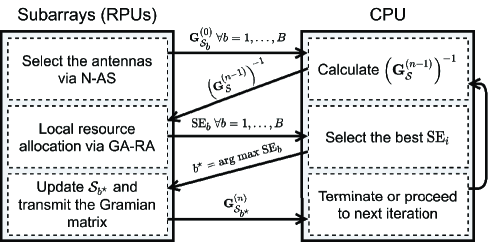
Figure 3: Proposed DGA-RA procedure steps with coordination between the CPU and the RPUs. The superscript $(n)$ denotes the $n$-th iteration.

After performing local AS, each subarray transmits their achieved SE values to the CPU. The CPU updates the AS indices of the subarray that has achieved the maximum SE values at the iteration $n$. Then, the CPU requests the subarray Gramian matrix of the updated subarray, and recalculates the inverse of the array Gramian matrix, $(\mathbf{G}_{\mathcal{S}}^{(n)})^{-1}$. The process can be executed iteratively following the scheme depicted in Fig. 3.

The GA implemented in the DGA-RA procedure is similar to that one described in the Algorithm 2, except for some details at the optimization variables encoding and the crossover phase. About the individual encoding, the optimization variables at each subarray are reduced from $M$ to $M_{b}$, since local AS is performed at each RPU. In addition, as the optimization variables consider only one subarray at each RPU, the individuals have two chromosomes: one represented by the first $M_{b}/2$ genes, and another composed by the remaining genes.

Due to this new chromosome definition, one further procedure after the crossover phase is required to preserve the solution’s feasibility. The chosen method is to deactivate antennas of individuals with more than $N_{b}$ antennas in a random fashion until they become feasible.

IV Antenna Selection Procedures

Two techniques to perform antenna selection are presented in the sequel, the DL sum-capacity maximization antenna selection (SCMAX-AS) and the N-AS method, proposed respectively in [14], [7]. The goal of solving only the antenna selection problem is to decouple the two RA problems associated to (15) aiming at obtaining tractable formulations.

IV-A Antenna Selection for DL Sum-Capacity Maximization

Firstly, we analize equal power allocation (EPA) strategy, i.e. $\mathbf{P}=\frac{P_{\max}}{K}\mathbf{I}_{K}$, intended to obtain a manageable optimization problem. The problem of selecting the set of active antennas in order to maximize the DL sum-capacity with the constraints of maximum number of RF transceivers and subarray connections is formulated as [14]:

$$\underset{\mathbf{D}}{\textrm{maximize}} \hskip 14.22636pt{C_{\textsc{epa}}=\log_{2}\textrm{det}\left(\mathbf{I}_{K}+\frac{P_{\max}}{K\sigma_{z}^{2}}\mathbf{H}^{H}\mathbf{DH}\right)}$$ (22a)

subject to $$\hskip 14.22636pt\sum_{m\in\mathcal{M}_{b}}D_{m}\leq N_{b},\;\forall b\in\{1,\dots,B\}$$ (22b)

$$\hskip 14.22636ptD_{m}\in\{0,1\},\;\forall m\in\{1,\dots,M\}$$ (22c)

Despite the concavity of the objective function in (22a) [13], the problem (22) is not convex due to the binary constraint in (22c). Hence, we define a convex relaxation of (22) by taking the variables $D_{m}$ in the range $(0,1)$. This new problem, which can be solved with convex optimization tools, has the constraint (22c) replaced by

$$0\leq D_{m}\leq 1,\;\forall m\in\{1,\dots,M\}$$ (23)

Notice that the solution of the convex relaxation results in non-binary values for the active antenna indicators $D_{m}$, which is outside the original problem domain.

One method for performing the antenna selection by solving the convex relaxation is to activate the $N_{b}$ antennas with the highest $D_{m}$ values at each subarray. This procedure is named in this work as SCMAX-AS, and is followed by the OPA policy in eq. (13). This AS procedure gives near-optimal results, except for $N\ll M$ [14]. Therefore, in a XL-MIMO system where the number of available RF transceivers is much less than the array antennas, the achieved system SE with the SCMAX-AS algorithm will be sub-optimal.

IV-B Norm-Based Antenna Selection (N-AS)

The N-AS procedure focus on selecting the subset of $N_{b}$ antennas with the highest channel vector norm values [7]. We adopt this method to initiate the population of the GA-based procedures due to its low computational cost. The N-AS method solves the optimization problem formulated as

$$\underset{\mathbf{D}}{\textrm{maximize}} \hskip 14.22636pt\Pi=\sum_{m=1}^{M}D_{m}\|\mathbf{\underline{h}}_{m}\|_{2}^{2}$$ (24a)

subject to $$\hskip 14.22636pt\sum_{m\in\mathcal{M}_{b}}D_{m}\leq N_{b},\;\forall b\in\{1,\dots,B\}$$ (24b)

$$\hskip 14.22636ptD_{m}\in\{0,1\},\;\forall m\in\{1,\dots,M\}$$ (24c)

where the objective function consists of the sum of the squared norms of the channel vectors associated to the selected antennas.

The problem (24) can be solved quickly by selecting the $N_{b}$ antennas with the highest channel vector norms at each subarray. After selection, the PA is performed by the OPA policy in (13).

V Complexity Analysis

The complexity of the presented procedures is evaluated in terms of the number of symbols required for channel acquisition, the size of the coordination data exchanged between the RPUs and the CPU, and the number of flops during execution.

V-A Training

In the following, we analyze the procedures in terms of training symbols for CSI acquisition. The length of the mutually orthogonal pilot signals used to estimate the channel vectors at the BS depends on: a) the number of users; b) the number of available RF transceivers; c) the number of antennas at the BS.

The number of symbols to acquire the entire channel matrix, required in all the presented procedures except in the N-AS, is $K\left\lceil\frac{M}{N}\right\rceil$. Particularly, the N-AS algorithm requires only the knowledge of the channel vector norms for selection. For this reason, the N-AS can be implemented without explicit channel estimation, supported by physical power-meters [21]. With this implementation, the N-AS requires a total of $2K$ symbols to operate. From this total, $K$ symbols are required to estimate the norms of the channel vectors, and the remaining $K$ symbols are used to estimate the channel vectors associated to the selected antennas.

V-B Coordination Data Size

The coordination data is defined as the data originated at the RPUs that is required at the CPU during the RA procedures. Determining the coordination data size is crucial since it can grow tremendously in the XL-MIMO scenario. In practical implementations, techniques as data compression helps alleviating the high interconnection bandwidth associated to the coordination data. However, such kind of consideration and optimization are out of the scope of this work.

Table II contains the coordination data size associated to the considered RA procedures, detailing the type of required data in each one. The GA-RA and SCMAX-AS procedures require the entire channel matrix at the CPU, while the DGA-RA one relies on the subarrays Gramian matrices. On the other hand, the N-AS procedure does not require any CSI knowledge at the CPU for antenna selection purpose, being the most appealing technique in terms of the coordination data size.

Table II: Coordination data exchanged between the RPUs and the CPU

Procedure	Implementation	Data type	Data size
GA-RA	Centralized	Channel matrix	$MK$
SCMAX-AS [14]	Centralized	Channel matrix	$MK$
N-AS [7]	Totally distributed	–	–
DGA-RA	Quasi-distributed	Gramian matrix	$(B+N_{\rm it})K^{2}$

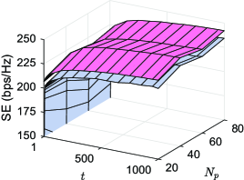
(a) Varying $N_{p}$

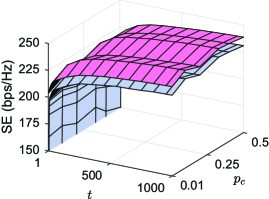
(b) Varying $p_{c}$

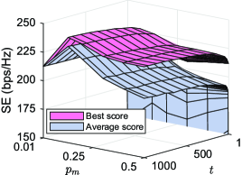
(c) Varying $p_{m}$

Figure 4: Convergence of the GA-RA with the number of generations $t$ varying the GA input parameters $N_{p}$, $p_{c}$ and $p_{m}$. The ”best” and ”average” SE surfaces are obtained over 20 realizations. In each plot, the values of the remaining input parameters are given in Table IV.

V-C Number of Flops

The third complexity metric is the number of flops executed by each procedure. The complexity analyses for the N-AS and the GA-based AS algorithms are as follows. The SCMAX-AS procedure is not considered due to the high complexity associated with computing the number of executed operations by the convex optimization solver.

N-AS: The operations executed at each subarray on the N-AS procedure consists of calculating the channel vectors’ norms then sorting the obtained values to get the $N_{b}$ largest ones. Assuming that the sorting operation has the complexity of the order $M_{b}\log(M_{b})$, the per-subarray flops for N-AS is

$$\mathcal{C}_{\textsc{n-as}}=M_{b}(2K-1)+M_{b}\log(M_{b})$$ (25)

GA-RA: The complexity of the GA-RA method is dominated by the number of operations required for the evaluation of the GA fitness function, eq. (11). At the first iteration, the algorithm evaluate the fitness function for $N_{p}$ individuals. During the remaining iterations, $(T-1)(N_{p}-N_{e})$ fitness function evaluations are done, where $T$ denotes the total number of generations.

As the OPA policy involves simple computations, the complexity of the fitness function is reduced to the inversion of the array Gramian matrix. The flops to compute the array Gramian matrix inverse is derived in Appendix B. From this result, the total flops for the GA-RA algorithm is

$$\mathcal{C}_{\textsc{ga-ra}}=\left[T(N_{p}-N_{e})+N_{e}\right]\left(\frac{7}{3}K^{3}+2NK^{2}-K^{2}\right)$$ (26)

DGA-RA: For the DGA-RA procedure, a similar approach to the one used for GA-RA can be followed. Despite that, the inverse of the array Gramian matrix is computed by the SMW formula, which is implemented with a different number of flops. The number of flops to obtain the inverse of the array Gramian matrix in the DGA-RA procedure is derived in Appendix C. Taking into account these differences and the fact that the DGA-RA procedure runs over $N_{\rm it}$ iterations, the total number of flops is given by:

$$\mathcal{C}_{\textsc{dga-ra}}=N_{\rm it}\left[T(N_{p}-N_{e})+N_{e}\right]\times$$ (27)

$$\hskip 42.67912pt\times\left[\frac{7}{3}N_{b}^{3}+2K^{3}+N_{b}^{2}(4K-1)\right.+$$

$$\hskip 56.9055pt+K^{2}(4N_{b}-2)+N_{b}^{2}(1-2K)+K\bigg{]}$$

VI Numerical Results

The numerical evaluations of the proposed methods as well as the benchmark techniques are presented in this section. The simulation system parameters are given in Table III. The users are randomly located inside a square cell of size $L$, and the BS is equipped with a uniform linear array (ULA) positioned on one side of the cell, as depicted in Fig. 1. Additionally, the users are random uniformly located at a distance in the range $(0.1L,L)$ from the array. Although the results in the following are obtained for the ULA, they can be easily extended to other array form factors, such as the uniform planar one.

Table III: Simulation parameters

Parameter	Value
Cell size	$L=30$ m
# Users	$K\in[1,217]$
Maximum transmitted power	$P_{\max}=230$ $\mu$W
Path-loss at the reference distance	$q_{0}=-35.3$ dB
Path-loss exponent	$\kappa=3$
Noise power	$\sigma_{z}^{2}=-96$ dBm
Uniform Linear Array (ULA) Setup
# Antennas	$M\in[32,2048]$
# RF transceivers	$N\in[64,256]$
# Subarrays	$B=\{2,4,8\}$
# Antennas per subarray	$M_{b}=M/B$
# RF transceivers per subarray	$N_{b}=N/B$

Before comparing the proposed techniques, it is necessary to tune the GA-RA and DGA-RA GA input parameters in order to obtain a suitable performance-complexity tradeoff. The input parameter $N_{p}$, $p_{c}$ and $p_{m}$ values are selected using the iterated local search algorithm [34]. The number of individuals for elitism is equal to 10% of the population size, and the number of tournaments is defined in order to fill the population after the elitism phase. Additionally, the stall convergence criterion parameter is approximately $30$% of the maximum number of generations. The selected parameters for the GA-based procedures are listed in Table IV. Notice that the DGA-RA procedure is set to run 10 times less generations than the GA-RA, since the number of optimization variables decrease from $M$ at the GA-RA to $M_{b}$ in the DGA-RA procedure.

Table IV: Genetic algorithm parameters

Symbol	Description	Parameter value
		GA-RA	DGA-RA
$N_{p}$	Population size	80	80
$N_{e}$	Elitism individuals	8	8
$N_{s}$	Tournaments	36	36
$p_{c}$	Crossover probability	0.33	0.35
$p_{m}$	Mutation probability	0.13	0.36
$T_{\max}$	Maximum generations	$10^{3}$	$10^{2}$
$T_{\rm stall}$	Stall generations	300	30

In Fig. 4, the quality of convergence of the GA-RA procedure is corroborated varying the parameters $N_{p}$, $p_{c}$ and $p_{m}$ independently. Each surface is computed by averaging the achieved scores over 20 realizations. These results on the best and average SE scores among the generations $t$ confirm the parameters’ values adopted in Table IV, while demonstrating a relative low tuning sensibility of the GA-RA convergence to the three input parameters.

Fig. 5 depicts the system SE achieved by the proposed RA procedures versus the number of available RF transceivers. In addition to the proposed solutions, the SE attained by random AS scheme and using all the $M$ antennas are plotted as the lower and upper performance bounds, respectively. The results consider $M=512$, $B=8$, $K=50$ and $N_{\rm it}\in\{5,16\}$ for the DGA-RA procedure. Observing the Fig. 5, one realize that the GA-based procedures achieve better SE results than the other ones. In the sequence, there are respectively the SCMAX-AS and N-AS. As expected, all the performance curves are upper and lower bounded by the SE achieved using full-array ZF and random AS, respectively. The SE gap between the procedures decreases as the number of RF transceivers increases. Analyzing the GA-based procedures, the DGA-RA achieves SE values tight to the GA-RA running with only five iterations. However, setting $N_{\rm it}=16$ makes the DGA-RA system SE values outperform marginally the ones obtained by the GA-RA procedure. Therefore, the quasi-distributed procedure can achieve a performance comparable, or even better, to the fully centralized approach by adopting a sufficient number of iterations.

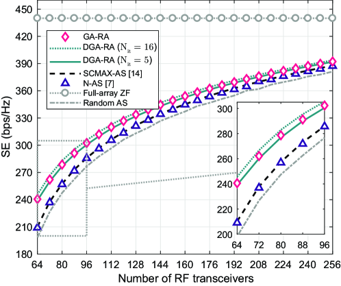
Figure 5: Comparison of SE vs the number of available RF transceivers. $M=512$, $B=8$, $K=50$ and, for the DGA-RA procedure $N_{\rm it}\in\{5,16\}$.

In the following, Fig. 6 depicts the system SE achieved by the proposed RA procedures versus the number of users. These numerical results consider $M=512$, $B=8$, $N=256$ and $N_{\rm it}\in\{5,16\}$ for the DGA-RA procedure. For better understanding, let $\mathcal{L}=K/N$ be the system effective loading factor. For all the proposed procedures, firstly the SE increases with $K$, assuming a decreasing behavior after a peak. This is due to the reduction of spatial degrees of freedom increasing the system loading factor, typically observed in linearly precoded systems [35]. Comparing the procedures, all of them get comparable SE values for a low loading factor. However, for high loading factor values, typically $\mathcal{L}=0.6$, the GA-RA and DGA-RA procedures get substantial better results. Again, the DGA-RA outperforms the GA-RA in terms of SE by setting $N_{\rm it}=16$. Combining the results in Figs. 5 and 6, we conclude that the GA-based procedures perform with higher SE gains over the other available AS schemes [7, 14] in crowded XL-MIMO scenarios, i.e., when the loading factor is high, $\mathcal{L}>0.25$.

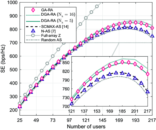
Figure 6: Comparison of SE vs the number of users. $M=512$, $B=8$, $N=256$ and, for the DGA-RA procedure $N_{\rm it}\in\{5,16\}$.

VI-A Complexity Analysis

The numerical results in the following cover the computational complexity of the proposed procedures. In Fig. 7 the coordination data size of the centralized procedures (GA-RA and SCMAX-AS) and the DGA-RA one versus the number of users is illustrated. The curves are evaluated by the expressions in Table II. The result considers $M\in\{512,2048\}$ and,for the DGA-RA procedure, $N_{\rm it}=16$ and $B\in\{2,4,8\}$. Comparing the RA approaches when the number of users is low, the quasi-distributed one get lower coordination data sizes than the centralized procedures. For higher numbers of users, the coordination data size associated to DGA-RA acquires larger values than the obtained by the centralized procedures. This point of inversion of behavior depends on the numbers of antennas, subarrays and iterations w.r.t. the DGA-RA procedure. It is worth mentioning that the coordination data size grows quadratically with $K$ for the DGA-RA procedure, while it grows linearly with $K$ for the centralized RA procedure.

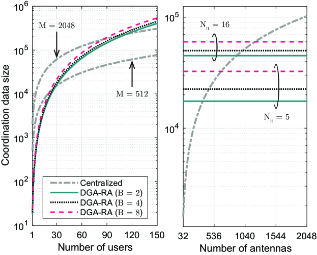
Figure 7: Coordination data size of the GA-based RA schemes vs the number of (a) users and (b) antennas. When it is not specified, $N_{\rm it}=16$ and $K=50$.

Fig. 7 depicts the coordination data size of the centralized procedures and the DGA-RA one versus the number of antennas in the BS. The results consider $K=50$ and, for the DGA-RA method, $N_{\rm it}\in\{5,16\}$ and $B\in\{2,4,8\}$. The coordination data size grows linearly with $M$ in the centralized procedures, while for the DGA-RA procedure, it does not depend on $M$. In fact, this is the primary aim for choosing a distributed RA technique in XL-MIMO, in which the BS is equipped with an asymptotically high number of antennas.

The next results are related to the complexity in terms of flops. Fig. 8 illustrates the number of flops per processing unit of the GA-based procedures versus the number of available RF transceivers. The curves are evaluated by the eqs. (26) and (27). Such results consider $K=50$ and, for the DGA-RA procedure, $B=8$ and $N_{\rm it}\in\{1,5,16\}$. For low numbers of RF transceivers, the flops’ values for the DGA-RA procedure are lower than the GA-RA algorithm. Again, after a point of inversion of behavior, the flops’ values for GA-RA get lower than the ones for the quasi-distributed procedure. This point of changing of behavior decreases as $N_{\rm it}$ increases.

The curves with the number of flops per processing unit of the GA-based procedures versus the number of users are depicted in Fig. 8. This result considers $N=256$ and, for the DGA-RA procedure, $B=8$ and $N_{\rm it}=\{1,5,16\}$. For low numbers of users, the flops’ values of the GA-RA procedure are lower than the ones get for the DGA-RA. However, this behavior inverts quickly, and the gap between the flops’ values for both centralized and distributed procedures becomes constant. This constant behavior for large $K$ is due to the fact that both eqs. (26) and (27) grow asymptotically with $K^{3}$.

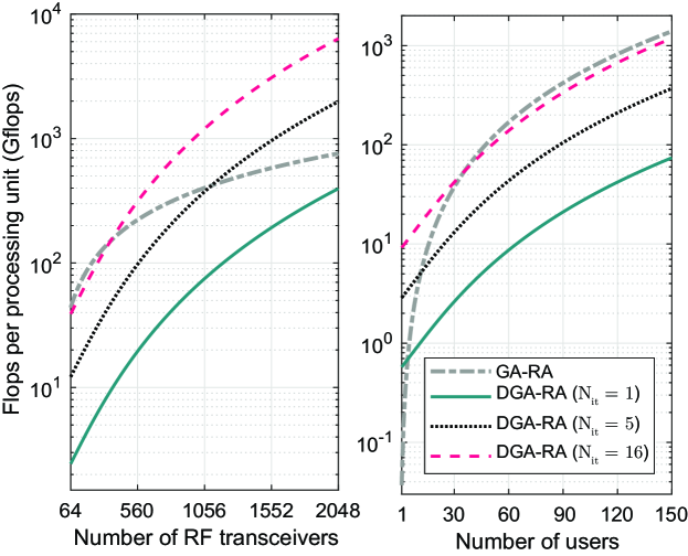
Figure 8: Flops per processing unit of the proposed GA-based procedures versus the number of (a) available RF transceivers and (b) users. $B=8$ and, when it is not specified, $K=50$ and $N=256$.

VII Conclusions

This works proposes a subarray switching architecture for the BS antenna array, while examining the problem of joint AS and PA optimization aiming at maximizing the SE of XL-MIMO systems with limited number of RF transceivers. Two GA-based near-optimal and low-complexity procedures are proposed. One is the centralized GA-RA, designed to operate with the entire channel matrix available at the CPU. The other is the quasi-distributed DGA-RA, based on the subarrays Gramian matrices. Both evolutionary metaheuristic optimization methods are analysed in terms of achieved SE, coordination data size and flops, and compared with benchmarks, including two procedures from the literature, the SCMAX-AS and the N-AS followed by optimal PA. Numerical results corroborate that the GA-based AS and PA procedures achieve high SE gains compared to the selected benchmarks, particularly in crowded XL-MIMO scenarios, i.e., when the effective loading factor $\mathcal{L}>0.25$. At the same time, the distributed DGA-RA method can outperform the other procedures with low-size coordination data and low computational complexity by taking the appropriate system operation settings.

Appendix A Local Computation of the Inverse of the Array Gramian Matrix via the Sherman-Morrison-Woodbury Formula

To compute the array Gramian matrix at the subarray $b$, the RPU must follow these two steps. Firstly, remove the contribution of the selected antennas at the subarray $b$ at the iteration $n-1$. Then, add the contribution of the selected antennas at the iteration $n$. Therefore, it needs to compute the inverse of the array Gramian matrix by the expression

$$\left(\mathbf{G}_{\mathcal{S}}^{(n)}\right)^{-1}=\left(\mathbf{G}_{\mathcal{S}}^{(n-1)}-\mathbf{G}_{\mathcal{S}_{b}}^{(n-1)}+\mathbf{G}_{\mathcal{S}_{b}}^{(n)}\right)^{-1}$$ (28)

which evaluation would be straightforward if all the terms were available at the subarray.

However, the subarray needs to compute $(\mathbf{G}_{\mathcal{S}}^{(n)})^{-1}$ knowing only $(\mathbf{G}_{\mathcal{S}}^{(n-1)})^{-1}$ and the local channel vectors, i.e. $\mathbf{\underline{h}}_{m}\;\forall m\in\mathcal{M}_{b}$ for the subarray $b$. Writing the subarray Gramian matrices of (28) in terms of the local channel matrices results in

$$-\mathbf{G}_{\mathcal{S}_{b}}^{(n-1)}+\mathbf{G}_{\mathcal{S}_{b}}^{(n)}$$

$$\hskip 28.45274pt=-\left(\mathbf{H}_{\mathcal{S}_{b}}^{(n-1)}\right)^{H}\mathbf{H}_{\mathcal{S}_{b}}^{(n-1)}+\left(\mathbf{H}_{\mathcal{S}_{b}}^{(n)}\right)^{H}\mathbf{H}_{\mathcal{S}_{b}}^{(n)}$$

$$\hskip 28.45274pt=\begin{bmatrix}-\left(\mathbf{H}_{\mathcal{S}_{b}}^{(n-1)}\right)^{H}&\left(\mathbf{H}_{\mathcal{S}_{b}}^{(n)}\right)^{H}\end{bmatrix}\begin{bmatrix}\mathbf{H}_{\mathcal{S}_{b}}^{(n-1)}\\ \mathbf{H}_{\mathcal{S}_{b}}^{(n)}\end{bmatrix}$$ (29)

From (28) and (29), it is possible to define the SMW formula variables, $\mathbf{A}^{-1}$, $\mathbf{U}$ and $\mathbf{V}^{H}$, in terms of the available information at the subarray as the eqs. (19), (20) and (21), respectively.

Appendix B Flops to Compute the Inverse of the Array Gramian Matrix via the Cholesky Decomposition

Initially, the computation of the array Gramian matrix is done by solving the product in (5), which costs $2K^{2}N-K^{2}$ flops [33]. Afterwards, define the Cholesky decomposition of the array Gramian matrix as

$$\mathbf{G}_{\mathcal{S}}=\mathbf{L}\mathbf{L}^{H}$$ (30)

where $\mathbf{L}$ is a lower triangular matrix. The computation of $\mathbf{L}$ can be done with $K^{3}/3$ flops [33]. Then, each column of the inverse of the Gramian matrix can be computed solving the set of linear systems below by backforward substitution,

$$\mathbf{L}\mathbf{L}^{H}\mathbf{x}=\mathbf{e}_{i},\;\forall i=1,\dots,K$$ (31)

where $\mathbf{e}_{i}$ denotes the canonical basis vector, i.e. a row vector with all entries equal to 0, except the entry $i$ which is equal to 1. Each linear system can be solved with $2K^{2}$ flops [33], totaling $2K^{3}$ flops for all the columns of $\mathbf{G}_{\mathcal{S}}^{-1}$. Therefore, the total flops for the array Gramian matrix computation and inversion is equal to

$$\mathcal{C}_{Chol.}=\frac{7}{3}K^{3}+2NK^{2}-K^{2}$$ (32)

Appendix C Flops to Compute the Inverse of the Array Gramian Matrix via the Sherman-Morrison-Woodbury Formula

To count the flops to compute the matrix inversion by the SMW formula, the eq. (18) is decomposed in six parts. The computations involved in each part and their respective flops are organized in Table V. The flops in Table V are counted assuming that the contribution of the selected antennas during the previous iteration is removed. Such assumption is reasonable since the expression in (28) can be done sequentially, by keeping only the terms $-\mathbf{G}_{\mathcal{S}_{b}}^{(n-1)}$ or $\mathbf{G}_{\mathcal{S}_{b}}^{(n)}$ at a time.

All the parts include only simple matrix multiplications and sums, except for the part $\mathbf{Q}_{3}$. This part can be efficiently computed by the Cholesky decomposition approach followed by the backforward substitution procedure described in Appendix B. Therefore, the total flops required to compute the inverse of the array Gramian matrix via the SMW formula is equal to

$$\mathcal{C}_{SMW}=\frac{7}{3}N_{b}^{3}+2K^{3}+N_{b}^{2}(4K-1)$$ (33)

$$\hskip 42.67912pt+K^{2}(4N_{b}-2)+N_{b}^{2}(1-2K)+K$$

Table V: Flops involved on the Sherman-Morrison-Woodbury formula computation

Symbol	Expression	Number of flops
$\mathbf{Q}_{1}$	$\mathbf{V}^{H}\mathbf{A}^{-1}$	$2N_{b}K^{2}-N_{b}K$
$\mathbf{Q}_{2}$	$\mathbf{I}+\mathbf{Q}_{1}\mathbf{U}$	$2N_{b}^{2}K-N_{b}^{2}+N_{b}$
$\mathbf{Q}_{3}$	$\mathbf{Q}_{2}^{-1}$	$7/3N_{b}^{3}$
$\mathbf{Q}_{4}$	$\mathbf{U}\mathbf{Q}_{3}$	$2N_{b}^{2}K-N_{b}K$
$\mathbf{Q}_{5}$	$\mathbf{I}-\mathbf{Q}_{4}\mathbf{Q}_{1}$	$2N_{b}K^{2}-K^{2}+K$
$\mathbf{Q}_{6}$	$\mathbf{A}^{-1}\mathbf{Q}_{5}$	$2K^{3}-K^{2}$

References

- [1] E. G. Larsson, O. Edfors, F. Tufvesson, and T. L. Marzetta, “Massive MIMO for next generation wireless systems,” IEEE Communications Magazine, vol. 52, no. 2, pp. 186–195, Feb. 2014.
- [2] E. D. Carvalho, A. Ali, A. Amiri, M. Angjelichinoski, and R. W. Heath, “Non-stationarities in extra-large-scale massive MIMO,” IEEE Wireless Communications, vol. 27, no. 4, pp. 74–80, Aug. 2020.
- [3] À. O. Martínez, E. De Carvalho, and J. Ø. Nielsen, “Towards very large aperture massive MIMO: A measurement based study,” in 2014 IEEE Globecom Workshops, Dec. 8–12 2014, pp. 281–286.
- [4] Z. Zhou, X. Gao, J. Fang, and Z. Chen, “Spherical wave channel and analysis for large linear array in LoS conditions,” in 2015 IEEE Globecom Workshops, Dec. 6–10 2015, pp. 1–6.
- [5] X. Li, S. Zhou, E. Björnson, and J. Wang, “Capacity analysis for spatially non-wide sense stationary uplink massive MIMO systems,” IEEE Transactions on Wireless Communications, vol. 14, no. 12, pp. 7044–7056, Dec. 2015.
- [6] A. Ali, E. D. Carvalho, and R. W. Heath, “Linear receivers in non-stationary massive MIMO channels with visibility regions,” IEEE Wireless Communications Letters, vol. 8, no. 3, pp. 885–888, Jun. 2019.
- [7] A. Garcia-Rodriguez, C. Masouros, and P. Rulikowski, “Reduced switching connectivity for large scale antenna selection,” IEEE Transactions on Communications, vol. 65, no. 5, pp. 2250–2263, May 2017.
- [8] Y. Gao, H. Vinck, and T. Kaiser, “Massive MIMO antenna selection: Switching architectures, capacity bounds, and optimal antenna selection algorithms,” IEEE Transactions on Signal Processing, vol. 66, no. 5, pp. 1346–1360, Mar. 2018.
- [9] K. Li, R. R. Sharan, Y. Chen, T. Goldstein, J. R. Cavallaro, and C. Studer, “Decentralized baseband processing for massive MU-MIMO systems,” IEEE Journal on Emerging and Selected Topics in Circuits and Systems, vol. 7, no. 4, pp. 491–507, Dec. 2017.
- [10] J. Rodríguez Sánchez, F. Rusek, O. Edfors, M. Sarajlić, and L. Liu, “Decentralized massive MIMO processing exploring daisy-chain architecture and recursive algorithms,” IEEE Transactions on Signal Processing, vol. 68, pp. 687–700, Jan. 2020.
- [11] A. Mueller, A. Kammoun, E. Björnson, and M. Debbah, “Linear precoding based on polynomial expansion: reducing complexity in massive MIMO,” EURASIP Journal on Wireless Communications and Networking, no. 63, pp. 1687–1499, Feb. 2016.
- [12] R. W. Heath, N. González-Prelcic, S. Rangan, W. Roh, and A. M. Sayeed, “An overview of signal processing techniques for millimeter wave MIMO systems,” IEEE Journal of Selected Topics in Signal Processing, vol. 10, no. 3, pp. 436–453, Apr. 2016.
- [13] A. Dua, K. Medepalli, and A. J. Paulraj, “Receive antenna selection in MIMO systems using convex optimization,” IEEE Transactions on Wireless Communications, vol. 5, no. 9, pp. 2353–2357, Sep. 2006.
- [14] X. Gao, O. Edfors, F. Tufvesson, and E. G. Larsson, “Massive MIMO in real propagation environments: Do all antennas contribute equally?” IEEE Transactions on Communications, vol. 63, no. 11, pp. 3917–3928, Nov. 2015.
- [15] P. Lin and S. Tsai, “Performance analysis and algorithm designs for transmit antenna selection in linearly precoded multiuser MIMO systems,” IEEE Transactions on Vehicular Technology, vol. 61, no. 4, pp. 1698–1708, May 2012.
- [16] A. Amiri, C. N. Manchon, and E. de Carvalho, “Deep learning based spatial user mapping on extra large MIMO arrays,” arXiv. 2002.00474, Feb. 2020.
- [17] J. C. Marinello, T. Abrão, A. Amiri, E. de Carvalho, and P. Popovski, “Antenna selection for improving energy efficiency in XL-MIMO systems,” IEEE Transactions on Vehicular Technology, vol. 69, no. 11, pp. 13 305–13 318, Nov. 2020.
- [18] H. Lu and W. Fang, “Joint transmit/receive antenna selection in MIMO systems based on the priority-based genetic algorithm,” IEEE Antennas and Wireless Propagation Letters, vol. 6, pp. 588–591, Dec. 2007.
- [19] J. Lain, “Joint transmit/receive antenna selection for MIMO systems: A real-valued genetic approach,” IEEE Communications Letters, vol. 15, no. 1, pp. 58–60, Jan. 2011.
- [20] B. Makki, A. Ide, T. Svensson, T. Eriksson, and M. Alouini, “A genetic algorithm-based antenna selection approach for large-but-finite MIMO networks,” IEEE Transactions on Vehicular Technology, vol. 66, no. 7, pp. 6591–6595, Jul. 2017.
- [21] J. R. Sánchez, J. Vidal Alegría, and F. Rusek, “Decentralized massive MIMO systems: Is there anything to be discussed?” in 2019 IEEE International Symposium on Information Theory, Jul. 7–12 2019, pp. 787–791.
- [22] A. Amiri, M. Angjelichinoski, E. de Carvalho, and R. W. Heath, “Extremely large aperture massive MIMO: Low complexity receiver architectures,” in 2018 IEEE Globecom Workshops, Dec. 9–13 2018, pp. 1–6.
- [23] A. Amiri, C. N. Manchón, and E. de Carvalho, “A message passing based receiver for extra-large scale mimo,” in 2019 IEEE 8th International Workshop on Computational Advances in Multi-Sensor Adaptive Processing (CAMSAP), 2019, pp. 564–568.
- [24] A. Amiri, S. Rezaie, C. N. Manchon, and E. de Carvalho, “Distributed receivers for extra-large scale MIMO arrays: A message passing approach,” arXiv. 2007.06930, Jul. 2020.
- [25] X. Yang, F. Cao, M. Matthaiou, and S. Jin, “On the uplink transmission of multi-user extra-large scale massive MIMO systems,” arXiv. 1909.06760, Nov. 2019.
- [26] D. A. Gore, R. U. Nabar, and A. Paulraj, “Selecting an optimal set of transmit antennas for a low rank matrix channel,” in 2000 International Conference on Acoustics, Speech, and Signal Processing, vol. 5, Jun. 5–9 2000, pp. 2785–2788.
- [27] A. F. Molisch, M. Z. Win, Yang-Seok Choi, and J. H. Winters, “Capacity of MIMO systems with antenna selection,” IEEE Transactions on Wireless Communications, vol. 4, no. 4, pp. 1759–1772, Jul. 2005.
- [28] S. Asaad, A. M. Rabiei, and R. R. Müller, “Massive MIMO with antenna selection: Fundamental limits and applications,” IEEE Transactions on Wireless Communications, vol. 17, no. 12, pp. 8502–8516, Dec. 2018.
- [29] C. Ouyang, Z. Ou, L. Zhang, P. Yang, and H. Yang, “Asymptotic upper capacity bound for receive antenna selection in massive MIMO systems,” in 2019 IEEE International Conference on Communications, May. 20–24 2019, pp. 1–6.
- [30] Z. Abdullah, C. C. Tsimenidis, G. Chen, M. Johnston, and J. A. Chambers, “Efficient low-complexity antenna selection algorithms in multi-user massive MIMO systems with matched filter precoding,” IEEE Transactions on Vehicular Technology, vol. 69, no. 3, pp. 2993–3007, Mar. 2020.
- [31] H. Siljak, I. Macaluso, and N. Marchetti, “Distributing complexity: A new approach to antenna selection for distributed massive MIMO,” IEEE Wireless Communications Letters, vol. 7, no. 6, pp. 902–905, Dec. 2018.
- [32] P. He, L. Zhao, S. Zhou, and Z. Niu, “Water-filling: A geometric approach and its application to solve generalized radio resource allocation problems,” IEEE Transactions on Wireless Communications, vol. 12, no. 7, pp. 3637–3647, Jun. 2013.
- [33] G. H. Golub and C. F. V. Loan, Matrix Computations. Baltimore, MD, USA: Johns Hopkins University Press, 2013.
- [34] E. Montero, M.-C. Riff, and B. Neveu, “A beginner’s guide to tuning methods,” Applied Soft Computing, vol. 17, pp. 39–51, Apr. 2014.
- [35] T. L. Marzetta, E. G. Larsson, H. Yang, and H. Q. Ngo, Fundamentals of Massive MIMO. Cambridge, Cambridgeshire, UK: Cambridge University Press, 2016.