intRinsic: an R Package for Model-Based Estimation of the Intrinsic Dimension of a Dataset

Abstract

This article illustrates intRinsic, an R package that implements novel state-of-the-art likelihood-based estimators of the intrinsic dimension of a dataset, an essential quantity for most dimensionality reduction techniques. In order to make these novel estimators easily accessible, the package contains a small number of high-level functions that rely on a broader set of efficient, low-level routines. Generally speaking, intRinsic encompasses models that fall into two categories: homogeneous and heterogeneous intrinsic dimension estimators. The first category contains the two nearest neighbors estimator, a method derived from the distributional properties of the ratios of the distances between each data point and its first two closest neighbors. The functions dedicated to this method carry out inference under both the frequentist and Bayesian frameworks. In the second category, we find the heterogeneous intrinsic dimension algorithm, a Bayesian mixture model for which an efficient Gibbs sampler is implemented. After presenting the theoretical background, we demonstrate the performance of the models on simulated datasets. This way, we can facilitate the exposition by immediately assessing the validity of the results. Then, we employ the package to study the intrinsic dimension of the Alon dataset, obtained from a famous microarray experiment. Finally, we show how the estimation of homogeneous and heterogeneous intrinsic dimensions allows us to gain valuable insights into the topological structure of a dataset.

Keywords: intrinsic dimension, nearest neighbors, likelihood-based method, heterogeneous intrinsic dimension, Bayesian mixture model, R

1 Introduction

Statisticians and data scientists are often called to manipulate, analyze, and summarize datasets that present high-dimensional and elaborate dependency structures. In numerous cases, these large datasets contain variables characterized by a considerable amount of redundant information. One can exploit these redundancies to represent a large dataset on a much lower-dimensional scale. This summarization procedure, called dimensionality reduction, is a fundamental step in many statistical analyses. For example, dimensionality reduction techniques grant the feasibility of otherwise challenging tasks such as large data manipulation and visualization by reducing computational time and memory requirements.

More formally, dimensionality reduction is possible whenever the data points take place on one or more manifolds characterized by a lower dimension than what has been observed initially. In this context, the word manifold is used to indicate a constraint surface embedded in high-dimensional space along which dissimilarities between data points are best represented (Tenenbaum et al., 2000; Lee et al., 2008). We call the dimension of a latent, potentially nonlinear manifold the intrinsic dimension (ID). Several other definitions of ID exist in the literature. For example, we can regard the ID as the minimal number of parameters needed to represent all the information contained in the data without significant information loss (Ansuini et al., 2019; Rozza et al., 2011; Bennett, 1969).
Intuitively, the ID is an indicator of the complexity of the features of a dataset. It is a necessary piece of information to have before attempting to perform any dimensionality reduction, manifold learning, or visualization tasks. Indeed, most dimensionality reduction methods would be worthless without a reliable estimate of the true ID they need to target: an underestimated ID value can cause needless information loss. At the same time, the reverse can lead to an unnecessary waste of time and computational resources (Hino et al., 2017). Beyond dimensionality reduction, ID estimation methods have been successfully employed, for instance, in studying physical systems (Mendes-Santos et al., 2021) and analyzing neural networks (Ansuini et al., 2019). For more examples of applications, see also Carter et al. (2010) and the references in the discussion in Bac et al. (2021).

Over the past few decades, a vast number of methods for ID estimation and dimensionality reduction have been developed. The algorithms can be broadly classified into two main categories: projection and geometric approaches. The former maps the original data to a lower-dimensional space. The projection function can be linear, as in the case of Principal Component Analysis (PCA) (Hotelling, 1933) or nonlinear, as in the case of Locally Linear Embedding (Roweis and Lawrence, 2000), Isomap (Tenenbaum et al., 2000), and the tSNE (Laurens and Geoffrey, 2009). For more examples, see Jollife and Cadima (2016) and the references therein. In consequence, there is a plethora of R packages that implement these types of algorithms. To mention some examples, one can use the packages RDRToolbox (Bartenhagen, 2020), lle (Kayo, 2006), Rtsne (Krijthe, 2015), and the classic princomp() function from the default package stats (R Core Team, 2021).

Instead, geometric approaches rely on the topology of a dataset, exploiting the properties of the distances between data points. Within this family, we can find fractal methods (Falconer, 2003), graphical methods (Costa and Hero, 2004), model-based likelihood approaches (Levina and Bickel, 2005), and methods based on nearest neighbors distances (Pettis et al., 1979). Also in this case, numerous packages are available: for example, for fractal methods alone there are fractaldim (Sevcikova et al., 2014), nonlinearTseries (Garcia, 2020), and tseriesChaos (Di Narzo, 2019), among others. For a recent review of the methodologies used for ID estimation we refer to Campadelli et al. (2015).

Given the abundance of approaches in this area, several R developers have also attempted to provide unifying collections of dimensionality reduction and ID estimation techniques. For example, remarkable ensembles of methodologies are implemented in the packages ider (Hino, 2017), dimred and coRanking (Kraemer et al., 2018), dyndimred (Cannoodt and Saelens, 2020), IDmining (Golay and Kanevski, 2017), and intrinsicDimension (Johnsson and Lund University, 2019). Among the various options, the package Rdimtools (You, 2020b) stands out, implementing 150 different algorithms, 17 of which are exclusively dedicated to ID estimation (You, 2020a). Finally, it is worth mentioning that there are also Python packages implementing different methods for ID estimation: two prominent examples are scikit-learn (Bac et al., 2021) and DADApy (Glielmo et al., 2022). See Section B of the Appendix for more details.

In this paper, we introduce and discuss the R package intRinsic (version 0.2.2). The package is openly available from the Comprehensive R Archive Network (CRAN) at https://CRAN.R-project.org/package=intRinsic, and can be installed by running

R> install.packages("intRinsic")

Future developments and updates will be uploaded both on CRAN and GitHub at https://github.com/Fradenti/intRinsic.

The package implements the two nearest neighbors (TWO-NN), the generalized ratio ID estimator (GRIDE), and the heterogeneous ID algorithm (HIDALGO) models, three state-of-the-art ID estimators recently introduced in Facco et al. (2017); Denti et al. (2022) and Allegra et al. (2020), respectively. These methods are likelihood-based estimators that rely on the theoretical properties of the distances among nearest neighbors. The first two models estimate a global, unique ID of a dataset and are implemented under both the frequentist and Bayesian paradigms. Moreover, one can exploit these models to study how the ID depends on the scale of the neighborhood considered for its estimation. On the contrary, HIDALGO is a Bayesian mixture model that allows for the estimation of clusters of points characterized by heterogeneous ID. In this article, we focus our attention on the exposition of TWO-NN and HIDALGO, and we discuss the pros and cons of both models with the aid of simulated data. More details about the additional routines, such as GRIDE, are reported in Section A of the Appendix. Finally, in Section B of the Appendix, we elaborate more on the strengths and weaknesses of the methods implemented in intRinsic in comparison to the other existing packages.

Broadly speaking, the package contains two sets of functions, organized into high-level and low-level routines. The former set contains user-friendly and straightforward R functions. Our goal is to make the package as accessible and intuitive as possible by automating most tasks. The low-level routines are not exported, as they represent the package’s core. The most computationally-intensive low-level functions are written in C++, exploiting the interface with R provided by the packages Rcpp and RcppArmadillo (Eddelbuettel and François, 2011; Eddelbuettel and Sanderson, 2014). The C++ implementation considerably speeds up time-consuming tasks, like running the Gibbs sampler for the Bayesian mixture model HIDALGO. Moreover, intRinsic is well integrated with external R packages. For example, we enriched the package’s functionalities defining ad-hoc methods for generic functions like autoplot() from the ggplot2 package (Wickham, 2016) to produce the detailed graphical outputs.

The article is structured as follows. Section 2 introduces and describes the theoretical background of the TWO-NN and HIDALGO methods. Section 3 illustrates the basic usage of the implemented routines on simulated data. We show how to obtain, manipulate, and interpret the different outputs. Additionally, we assess the robustness of the methods by monitoring how the results vary when the input parameters change. Section 4 presents an application to a famous real microarray dataset. Finally, Section 5 concludes by discussing future directions and potential extensions to the package.

2 The modeling background

Let $\bm{X}$ be a dataset with $n$ data points measured over $D$ variables. We denote each observation as $x_{i}\in\mathbb{R}^{D}$, with $i=1,\ldots,n$. Despite being observed over a $D$-dimensional space, we suppose that the points take place on a latent manifold $\mathcal{M}$ with intrinsic dimension $d\leq D$. Generally, we expect that $d<<D$. Thus, we postulate that a low-dimensional data-generating mechanism can accurately describe the dataset.
Then, consider a single data point $x_{i}$. Starting from this point, one can order the remaining $n-1$ observations according to their distance from $x_{i}$. This way, we obtain a list of nearest neighbors (NNs) of increasing order. Formally, let $\Delta:\mathbb{R}^{D}\times\mathbb{R}^{D}\rightarrow\mathbb{R}^{+}$ be a generic distance function between data points. We denote with $x_{i}^{(l)}$ the $l$-th NN of $x_{i}$ and with $r_{i,l}=\Delta\left(x_{i},x_{i}^{(l)}\right)$ their distance, for $l=1,\ldots,n-1$. Given the sequence of NNs for each data point, we can define the volume of the hyper-spherical shell enclosed between two successive neighbors of $x_{i}$ as

$$\nu_{i,l}=\omega_{d}\left(r_{i,l}^{d}-r_{i,l-1}^{d}\right),\quad\quad\text{for }l=1,\ldots,n-1,\;\text{ and }\;i=1,\ldots,n,$$ (1)

where $d$ is the dimensionality of the latent manifold in which the points are embedded (the ID) and $\omega_{d}$ is the volume of the $d$-dimensional hyper-sphere with unitary radius. For this formula to hold, we need to set $x_{i,0}\equiv x_{i}$ and $r_{i,0}=0$. We provide a visual representation of the introduced quantities in Figure 1 for $l=1,2$, which depicts the three-dimensional case.

From a modeling perspective, we assume that the dataset $\bm{X}$ is a realization of a Poisson point process characterized by density function $\rho\left(x\right)$. Facco et al. (2017) showed that the hyper-spherical shells defined in Equation 1 are the multivariate extension of the well-known inter-arrival times (Kingman, 1992). Indeed, they proved that under the assumption of homogeneity of the Poisson point process, i.e., $\rho(x)=\rho\>\>\forall x$, all the $\nu_{i,l}$’s are independently drawn from an Exponential distribution with rate equal to the density $\rho$: $\nu_{i,l}\sim Exp(\rho)$, for $l=1,\ldots,n-1,$ and $i=1,\dots,n$. This fundamental result motivates the derivation of the estimators we will introduce in the following.

Figure 1: An illustration in three dimensions of the quantities involved in the TWO-NN modeling framework. The central dot represents the $i$-th data point. The selected observation is connected by dashed lines, representing the distances $r_{i,j}$, $j=1,2,3$, to its first three NNs. The different spherical shells have volumes $v_{i,j}$, $j=1,2,3$.

2.1 The TWO-NN estimator

Building on the distribution of the hyper-spherical shells, Facco et al. (2017) noticed that if the intensity of the underlying Poisson point process is assumed to be constant on the scale of the second NN, the following distributional result holds:

$$\mu_{i,1,2}=\frac{r_{i,2}}{r_{i,1}}\sim Pareto(1,d),\quad\quad\mu_{i}\in\left[1,+\infty\right)\quad\quad i=1,\ldots,n.$$ (2)

In other words, if the intensity of the Poisson point process that generates the data can be regarded as locally constant (on the scale of the second NN), the ratio of the first two NN distances from each point is Pareto distributed. Recall that the Pareto random variable is characterized by a scale parameter $a$, shape parameter $b$, and density function $f_{X}(x)=ab^{a}x^{-a-1}$ defined over $x\in\left[a,+\infty\right)$. Remarkably, Equation 2 states that the ratio ${r_{i,2}}/{r_{i,1}}$ follows a Pareto distribution with scale $a=1$ and shape $b=d$, i.e., the shape parameter can be interpreted as the ID of the dataset. Estimating $d$ by exploiting the ratios of distances between each point and its first two NNs is the core of the TWO-NN procedure.

One can also attain more general results by considering ratios of distances with NNs of generic orders. A generalized ratio will be denoted with $\mu_{i,n_{1},n_{2}}=r_{i,n_{2}}/r_{i,n_{1}}$ for $i=1,\ldots,n$. Here, $n_{1}$ and $n_{2}$ are the NN orders, integer numbers that need to comply with the following constraint: $1\leq n_{1}<n_{2}\leq n$. In this paper, we will mainly focus on methods involving the ratio of the first two NN distances. The generalized ratios will be only mentioned when discussing the function compute_mus(), for the sake of completeness. Therefore, to simplify the notation, we will write $\mu_{i}=\mu_{i,1,2}$ and $\bm{\mu}=\left(\mu_{i}\right)_{i=1}^{n}$.
Once the vector $\bm{\mu}$ is computed, we can employ different estimation techniques for the TWO-NN model. All of the following methods can be called via the intRinsic function twonn(). The reader can find examples of its usage in Section 3.3.

Linear estimator. Facco et al. (2017) proposed to estimate the ID via the linearization of the Pareto c.d.f. $F({\mu_{i}})=(1-\mu_{i}^{-d})$. The estimate $\hat{d}_{OLS}$ is obtained as the solution of

$$-\log(1-\hat{F}(\mu_{(i)}))=d\log(\mu_{(i)}),$$ (3)

where $\hat{F}(\cdot)$ denotes the empirical c.d.f. of the sample and the $\mu_{(i)}$’s are the ratios defined in Equation 2 sorted by increasing order. The authors also suggested trimming from $\bm{\mu}$ a percentage $c_{TR}$ of the most extreme values to obtain a more robust estimation. This choice is justified because the extreme ratios often correspond to observations that do not comply with the local homogeneity assumption.

Maximum likelihood estimator. In a similar spirit, Denti et al. (2022) took advantage of the distributional results in Equation 2 to derive a simple maximum likelihood estimator (MLE) and the corresponding confidence interval (CI). Trivially, the (unbiased) MLE for the shape parameter of a Pareto distribution is given by:

$$\hat{d}=\frac{n-1}{\sum_{i}^{n}\log(\mu_{i})},$$ (4)

while the CI of level (1-$\alpha$) is defined as

$$CI(d,1-\alpha)=\left[\frac{\hat{d}}{q^{1-\alpha/2}_{IG_{n,(n-1)}}},\frac{\hat{d}}{q^{\alpha/2}_{IG_{n,(n-1)}}}\right],$$ (5)

where $q^{\alpha/2}_{IG_{a,b}}$ denotes the quantile of order $\alpha/2$ of an Inverse-Gamma distribution of shape $a$ and scale $b$.

Bayesian estimator. It is also straightforward to derive an estimator according to a Bayesian perspective (Denti et al., 2022), obtained with the specification of a prior distribution on the shape parameter $d$. The most natural prior to choose is a conjugate $d\sim Gamma(a,b)$. It is immediate to derive the posterior distribution for the shape parameter:

$$d|\bm{\mu}\sim Gamma\left(a+n,b+\sum_{i=1}^{n}\log(\mu_{i})\right).$$ (6)

With this method, one can quickly recover the principal quantiles of the posterior distribution and obtain point estimates and uncertainty quantification with a credible interval (CRI) of level $\alpha$.

2.2 HIDALGO: the heterogeneous intrinsic dimension algorithm

The TWO-NN model implicitly assumes the existence of a single manifold. However, postulating a global, unique ID value for the entire dataset can often be limiting, especially when the data present complex dependence structures among variables. To extend the previous modeling framework, one can imagine that the data points are divided into clusters, each belonging to a latent manifold with its specific ID. Allegra et al. (2020) employed this heterogeneous ID estimation approach in their model: the heterogeneous ID algorithm (HIDALGO). The authors proposed as density function of the generating point process a mixture of $K$ distributions defined on $K$ different latent manifolds, expressed as $\rho\left(\bm{x}\right)=\sum_{k=1}^{K}\pi_{k}\rho_{k}\left(\bm{x}\right)$, where $\bm{\pi}=\left(\pi_{1},\ldots,\pi_{K}\right)$ is the vector of mixture weights. This assumption induces a mixture of Pareto distributions as the distribution of the ratios $\mu_{i}$’s:

$$f(\mu_{i}|\bm{d},\bm{\pi})=\sum_{k=1}^{K}\pi_{k}\>d_{k}\mu_{i}^{-(d_{k}+1)},\quad\quad i=1,\ldots,n,$$ (7)

where $\bm{d}=\left(d_{1},\ldots,d_{K}\right)$ is the vector of ID parameters. Allegra et al. (2020) adopted a Bayesian perspective, specifying independent Gamma priors for each element of $\bm{d}:$ $d_{k}\sim Gamma(a_{d},b_{d})$, and a Dirichlet prior for the mixture weights $\bm{\pi}\sim Dirichlet(\alpha_{1},\ldots,\alpha_{K})$. Regarding the latter, we suggest setting $\alpha_{1}=\ldots=\alpha_{K}=\alpha<0.05$, fitting a sparse mixture model as indicated by Malsiner-Walli et al. (2017). This prior specification encourages the data to populate only the necessary number of mixture components. Thus, we see $K$ as an upper bound on the number of active clusters $K^{*}\leq K$.

Unfortunately, a model-based clustering approach like the one presented in Equation 7 is ineffective at modeling the distance ratios. The problem lies in the fact that the different Pareto kernels have extremely similar shapes. Therefore, Pareto densities with varying shape parameters can fit the same data points equally well, compromising the clustering allocation and the consequent ID estimation. Even when considering very diverse shape parameters, the right tails of the resulting Pareto distributions overlap to a great extent. This issue is evident in Figure 2, where we depict examples of various $Pareto(1,d)$ densities.

Figure 2: Density functions of Pareto distributions characterized by different shape parameters.

To address this problem, Allegra et al. (2020) introduced a local homogeneity assumption, assuming that neighboring points are more likely to be part of the same latent manifold. To incorporate this idea in the model, the authors added an extra penalizing term in the likelihood. We now summarize their approach.
First, they introduced the latent membership labels $\bm{z}=(z_{1},\ldots,z_{n})$ to assign each observation to a cluster, where $z_{i}=k$ means that the $i$-th observation belongs to the $k$-th mixture component. Then, they defined the binary adjacency matrix $\mathcal{N}^{(q)}$, whose entries are $\mathcal{N}_{i,j}^{(q)}=1$ if the point $x_{j}$ is among the first $q$ NNs of $x_{i}$, and 0 otherwise. Finally, they assumed the following probabilities: $\mathbb{P}\left[\mathcal{N}_{i,j}^{(q)}=1|z_{i}=z_{j}\right]=\zeta_{1}$, with $\zeta_{1}>0.5$ and $\mathbb{P}\left[\mathcal{N}_{i,j}^{(q)}=1|z_{i}\neq z_{j}\right]=\zeta_{0}$, with $\zeta_{0}<0.5$. These probabilities are employed to define a distribution over the neighboring structure of each data point $x_{i}$: $\pi(\mathcal{N}_{i}^{(q)}|\bm{z})=\prod_{j=1}^{n}\zeta_{0}^{\mathds{1}_{z_{i}\neq z_{j}}}\zeta_{1}^{\mathds{1}_{z_{i}=z_{j}}}/\mathcal{Z}_{i}$, where $\mathcal{Z}_{i}$ is the normalizing constant and $\mathds{1}_{A}$ is the indicator function, equal to 1 when the event $A$ is true, 0 otherwise. A more technical discussion of this model extension and the validity of the underlying hypotheses can be found in the Supplementary Material of Allegra et al. (2020). For simplicity, we assume $\zeta_{0}=\zeta$ and $\zeta_{1}=1-\zeta$. The new likelihood becomes

$$\mathcal{L}\left(\mu_{i},\mathcal{N}^{(q)}|\bm{d},\bm{z},\zeta\right)=\>d_{z_{i}}\mu_{i}^{-(d_{z_{i}}+1)}\times\prod_{i=1}^{n}\frac{\zeta^{\mathds{1}_{z_{i}\neq z_{j}}}(1-\zeta)^{\mathds{1}_{z_{i}=z_{j}}}}{\mathcal{Z}_{i}},\quad\quad z_{i}|\bm{\pi}\sim Cat_{K}(\bm{\pi}),$$ (8)

where $Cat_{K}$ denotes a Categorical distribution over the set $\{1,\ldots,K\}$. A closed-form for the posterior distribution is not available, so we rely on MCMC techniques to simulate a posterior sample.

In our package, this Bayesian mixture model is implemented by the function Hidalgo(). For the ID parameters, we use conjugate Gamma prior specifications or variations thereof to account for modeling inconsistencies. For example, when the nominal dimension $D$ is low, the unbounded support of a Gamma prior may provide unrealistic results, where the posterior distribution assigns positive density to the interval $\left(D,+\infty\right)$. Santos-Fernandez et al. (2022) proposed to employ a more informative prior for $\bm{d}$:

$$\pi(d_{k})=\hat{\rho}\cdot d_{k}^{a-1}\exp^{-bd_{k}}\frac{\mathbbm{1}_{(0,D)}}{\mathcal{C}_{a,b,D}}+(1-\hat{\rho})\cdot\delta_{D}(d_{k})\quad\forall k,$$ (9)

where they denoted the normalizing constant of a $Gamma(a,b)$ truncated over $\left(0,D\right]$ with $\mathcal{C}_{a,b,D}$. That is, the prior distribution for $d_{k}$ is a mixture between a truncated Gamma distribution over $\left(0,D\right]$ and a point mass located at $D$. The parameter $\rho$ denotes the mixing proportion. When $\rho=1$, the distribution in Equation 9 reduces to a simple truncated Gamma. Both approaches are implemented in intRinsic, but we recommend using the latter. We report the details of the implemented Gibbs sampler in Section C of the Appendix, while in Section F we comment more on the concept of heterogeneous ID estimation related to global and local ID definitions.

3 Examples using intRinsic

This section illustrates the main routines of the intRinsic package. Here, we indicate the number of observations and the observed nominal dimension with n and D, respectively. Also, $\mathcal{N}_{k}(m,\Sigma)$ represents a multivariate normal distribution of dimension $k$, mean $m$, and covariance matrix $\Sigma$. Moreover, let $\mathcal{U}^{(k)}_{\left(a,b\right)}$ represent a multivariate Uniform distribution with support $\left(a,b\right)$ in $k$ dimensions. Finally, we denote with $\mathbb{I}_{k}$ an identity matrix of dimension $k$.
To start, we load our package by running:

R> library("intRinsic")

3.1 Simulated datasets

To illustrate how to apply the different ID estimation techniques available in the package, we will use three simulated datasets: Swissroll, Hypercube, and GaussMix. This way, we can compare the results of the experiments with the ground truth. One can generate the exact replica of the three simulated datasets used in this paper by running the code reported below.

The first dataset, Swissroll, is obtained via the classical Swissroll transformation $\mathcal{S}:\mathbb{R}^{2}\rightarrow\mathbb{R}^{3}$ defined as $\mathcal{S}(x,y)=(x\cos(x),y,x\sin(x))$, where each pair of points $\left(x,y\right)$ is sampled from two independent Uniform distributions on $\left(0,10\right)$. To simulate such a dataset, we can use the intRinsic function Swissroll(), specifying the number of observations n as the input parameter.

R> set.seed(123456)
R> Swissroll <- Swissroll(n = 1000)

The second dataset, Hypercube, contains a cloud of 500 points sampled from $\mathcal{U}^{(5)}_{\left(0,1\right)}$ embedded in an eight-dimensional space $\mathbb{R}^{8}$. To fill the gap between the nominal dimension (8) and the ID (5), we add three columns of zeros.

R> HyperCube  <- cbind(replicate(5, runif(500)), 0, 0, 0)

Lastly, the dataset GaussMix contains 1500 data points generated from three random variables all contained in a five-dimensional Euclidean space. More precisely, we consider a bivariate random variable defined as $X_{1}=(X_{0},3X_{0})$ where $X_{0}\sim\mathcal{N}_{1}(-5,1)$, and the three- and five-dimensional variables

$$X_{2}\sim\mathcal{N}_{3}(0,\mathbbm{I}_{3}),\quad X_{3}\sim\mathcal{N}_{5}(5,\mathbbm{I}_{5}).$$

We embed each of them in a five-dimensional space by adding the corresponding number of columns of zeros, as we did for the HyperCube dataset.

R> x0 <- rnorm(500, mean = -5, sd = 1)
R> x1 <- cbind(x0, 3 * x0, 0, 0, 0)
R> x2 <- cbind(replicate(3, rnorm(500)), 0, 0)
R> x3 <- replicate(5, rnorm(500, 5))
R> GaussMix <- rbind(x1, x2, x3)
R> class_GMix <- rep(c("A", "B", "C"), rep(500, 3))

Next, we need to establish the true values of the ID for the different datasets. Scatterplots are useful exploratory tools to spot any clear dependence across the columns of a dataset. For example, if we plot all the possible two-dimensional scatterplots from the Swissroll dataset, we obtain Figure 3. The different panels show that two of the three coordinates are free, and we can recover the last coordinate as a function of the others. Therefore, the ID of Swissroll is equal to 2. Moreover, from the description of the data simulation, it is also evident that the ID is equal to 5 for the Hypercube dataset. However, it is not as simple to figure out the value of the true ID for GaussMix, given the heterogeneity of its data-generating mechanism. Table 1 summarizes the sample sizes along with the true nominal dimensions D and IDs that characterize the three datasets.

Figure 3: Scatterplots of the three variables in the Swissroll dataset. The dependence among the coordinates $x$ and $z$ is evident.

Name	n	D	ID
Swissroll	1000	3	2
Hypercube	500	8	5
GaussMix	1500	5	?

Table 1: Summary of the characteristics of the three simulated datasets.

3.2 Ratios of nearest neighbors distances

The ratios of NN distances constitute the core quantities on which the theoretical development presented in Section 2 is based. We can compute the ratios $\mu_{i}$ defined in Equations 2 with the function compute_mus(). All in all, the function can also compute the generalized ratios $\bm{\mu}_{n_{1},n_{2}}$, where n1 < n2, as presented in Section 2.1. In fact, the function needs the following arguments:

• X: a dataset of dimension n$\times$D of which we want to compute the distance ratios;

• dist_mat: a n$\times$n symmetric matrix containing the distances between data points which one can pass instead of X;

• n1 and n2: the orders of the closest and furthest nearest neighbors to consider, respectively. As default, n1 = 1 and n2 = 2.

The function has two additional arguments, Nq and q, that we will introduce later in Section 3.4 when we will illustrate the HIDALGO model.
Note that the specification of dist_mat overrides the argument passed as X. Instead, if the distance matrix dist_mat is not specified, generate_mus() relies on the function get.knn() from the package FNN (Beygelzimer et al., 2019), which implements fast NN-search algorithms on the original dataset.

The main output of the function is the vector of ratios $\bm{\mu}_{n_{1},n_{2}}$, an object of class mus for which appropriate print() and plot() methods are defined. To use the function, we can easily write:

R> mus_Swissroll <- compute_mus(X = Swissroll)
R> mus_HyperCube <- compute_mus(X = HyperCube)
R> mus_GaussMix <- compute_mus(X = GaussMix)

Calling the function with default arguments produces $\bm{\mu}=\bm{\mu}_{1,2}$. To explicitly compute generalized ratios, we need to specify the NN orders n1 and n2. Here, we report two different examples:

R> mus_Swissroll_1 <- compute_mus(X = Swissroll, n1 = 5, n2 = 10)
R> mus_HyperCube_1 <- compute_mus(X = HyperCube, n1 = 5, n2 = 10)
R> mus_GaussMix_1 <- compute_mus(X = GaussMix, n1 = 5, n2 = 10)

and

R> mus_Swissroll_2 <- compute_mus(X = Swissroll, n1 = 10, n2 = 20)
R> mus_HyperCube_2 <- compute_mus(X = HyperCube, n1 = 10, n2 = 20)
R> mus_GaussMix_2 <- compute_mus(X = GaussMix, n1 = 10, n2 = 20)
R> mus_GaussMix_2

Ratio statistics mu’s:
NN orders: n1 = 10, n2 = 20.
Sample size: 1500.
Nominal Dimension: 5.

Figure 4: Histograms of the ratios $\bm{\mu}_{n_{1},n_{2}}$ for the Swissroll, Hypercube, and GaussMix datasets. The shape of the histograms in the first column suggests that a Pareto distribution could be a good fit, according to the TWO-NN model.

The histograms of the computed ratios are presented in Figure 4. The panels in each row correspond to different datasets, while the varying NN orders are reported by column. The horizontal axes are truncated over the interval $\left[0,4\right]$ to improve the visualization. The histograms present the right-skewed shape typical of the Pareto distribution. However, some ratios could assume extreme values, especially when low values of NN orders are chosen. To provide an example, in Table 2 we display the summary statistics of the three vectors of ratios computed on GaussMix. The maximum in the first line has a high magnitude, but it significantly reduces when higher NN orders are considered. It is also interesting to observe how the distribution for the ratios of GaussMix when $\texttt{n1}=10$ and $\texttt{n2}=20$ (bottom-right panel) is multimodal, a symptom of the presence of heterogeneous manifolds. We remark again that we will focus on the TWO-NN and HIDALGO models for the rest of the paper. Therefore, we will only use compute_mus() in its default specification, simply computing $\bm{\mu}=\left(\mu_{i}\right)_{i=1}^{n}$. The ratios of NNs of generic order are necessary when using the GRIDE model. See Section A of the Appendix and Denti et al. (2022) for more details.

n1	n2	Minimum	1st quartile	Median	Mean	3rd quartile	Maximum
1	2	1.0002	1.1032	1.3048	18.4239	1.9228	5874.3666
5	10	1.0234	1.1627	1.2858	1.5344	1.7043	6.9533
10	20	1.0472	1.1685	1.2613	1.4987	1.7250	4.0069

Table 2: Summary statistics of the generalized ratios obtained from the GaussMix dataset. Each row corresponds to a different combination of NN orders.

Finally, recall that the model is based on the assumption that a Poisson point process is the generating mechanism of the dataset. Ergo, the model cannot handle ties among data points. From a more practical point of view, if $\exists i\neq j$ such that $x_{i}=x_{j}$, the computation of $\mu_{i}$ would be unfeasible since $r_{i,1}=0$. We devised the function compute_mus() to automatically detect if duplicates are present in a dataset. In that case, the function removes the duplicates and provides a warning. We showcase this behavior with a simple example:

R> Dummy_Data_with_replicates <- rbind(
+     c(1, 2, 3), c(1, 2, 3),
+     c(1, 4, 3), c(1, 4, 3),
+     c(1, 4, 5) )
R> mus_shorter <- compute_mus(X = Dummy_Data_with_replicates)

Warning:
Duplicates are present and will be removed.

Original sample size: 5. New sample size: 3.

The function compute_mus() is at the core of many other high-level routines we use to estimate the ID. The following subsection shows how to implement the TWO-NN model to obtain a point estimate of a global, homogeneous ID accompanied by the corresponding CIs or CRIs.

3.3 Estimating a global ID value with TWO-NN

We showcase how to carry out inference on the ID with the TWO-NN model using linear, MLE, and Bayesian estimation methods. The low-level functions that implement these methods are twonn_mle(), twonn_linfit(), and twonn_bayes(), respectively. One can call these low-level functions via the high-level function twonn(). Regardless of the preferred estimation method, the twonn() function takes the following arguments: the dataset X or the distance matrix dist_mat (refer to previous input descriptions for more details), along with

• mus: the vector of second-to-first NN distance ratios. If this argument is provided, X and dist_mat will be ignored;

• method: a string stating the preferred estimation method. Could be "mle" (the default), "linfit", or "bayes";

• alpha: the confidence level (for "mle" and "linfit") or the posterior probability included in the CRI ("bayes");

• c_trimmed: the proportions of most extreme ratios to exclude from the analysis.

The object that the function returns is a list,characterized by a class that varies according to the selected estimation method. Tailored R methods have been devised to extend the generic functions print(), summary(), plot(), and autoplot() to interact with these new classes. The first element of the returned list always contains the estimates, while the others provide additional information about the chosen estimation process.

Linear estimator. We apply the linear estimator to the Swissroll dataset. As an example, we fit five linear models by setting method = "linfit", adopting different trimming proportions. The function summary() provides an informative recap of the estimation process. We show the results for lin_2 as an example.

R> lin_1 <- twonn(X = Swissroll, method = "linfit", c_trimmed = 0)
R> lin_2 <- twonn(X = Swissroll, method = "linfit", c_trimmed = 0.001)
R> lin_3 <- twonn(X = Swissroll, method = "linfit", c_trimmed = 0.01)
R> lin_4 <- twonn(X = Swissroll, method = "linfit", c_trimmed = 0.05)
R> lin_5 <- twonn(X = Swissroll, method = "linfit", c_trimmed = 0.1)
R> summary(lin_2)

Model: TWO-NN
Method: Least Squares Estimation
Sample size: 1000, Obs. used: 999. Trimming proportion: 0.1%
ID estimates (confidence level: 0.95)

| Lower Bound| Estimate| Upper Bound|
|-----------:|--------:|-----------:|
|    1.986659| 1.999682|    2.012705|

The results of these experiments are collected in Table 3. This first example allows us to comment on the trimming level to choose. Trimming the most extreme observations may be fundamental since outliers may distort the estimate. However, too much trimming would remove important information regarding the tail of the Pareto distribution, which is essential for the correct estimation of the ID. The estimates improve for very low levels of trimming but start to degenerate as more than 5% of observations are removed from the dataset.

Trimming percentage	0%	0.1%	1%	5%	10%
Lower bound	1.9524	1.9867	2.2333	2.5709	2.9542
Estimate	1.9669	1.9997	2.2457	2.5988	2.9974
Upper bound	1.9814	2.0127	2.2581	2.6267	3.0407

Table 3: Point estimates and relative CIs for the ID values retrieved from the Swissroll dataset with the linear estimator. Each column displays the results for a specific trimming level.

We can also visually assess the goodness of fit via a dedicated autoplot() function, which displays the data and the estimated regression line. The slope of the regression lines corresponds to the linear fit ID estimates. For example, we obtain the plots in Figure 5 with the following two lines of code:

R> autoplot(lin_1, title = "No trimming")
R> autoplot(lin_5, title = "10% trimming")

Figure 5: Swissroll dataset. Regression lines estimated from $-\log(1-\hat{F}(\mu_{i}))=d\log(\mu_{i})$ with no trimming (left panel) and 10% of trimmed observations (right panel).

MLE. A second way to obtain an ID estimate, along with its CI, is via MLE. The formulas implemented are presented in Equations 4 and 5. We compute the MLE by calling the low-level twonn_mle() function setting method = "mle". In addition to the previous arguments, one can also specify

• unbiased: logical, if TRUE the point estimate according to the unbiased estimator (where the numerator is $n-1$, as in Equation 4) is computed.

We compute the ID on Hypercube via MLE using different distance definitions: Euclidean, Manhattan, and Canberra. These distances are calculated with the dist() function of the stats package.

R> dist_Eucl_D2 <- dist(HyperCube)
R> dist_Manh_D2 <- dist(HyperCube, method = "manhattan")
R> dist_Canb_D2 <- dist(HyperCube, method = "canberra")

Other distance matrices can be employed as well. In this example, we also show how the widths of the CIs change by varying the confidence levels. We print the results stored in the object mle_12 as an example. We write:

R> mle_11 <- twonn(dist_mat = dist_Eucl_D2)
R> mle_12 <- twonn(dist_mat = dist_Eucl_D2, alpha = .99)
R> mle_21 <- twonn(dist_mat = dist_Manh_D2)
R> mle_22 <- twonn(dist_mat = dist_Manh_D2, alpha = .99)
R> mle_31 <- twonn(dist_mat = dist_Canb_D2)
R> mle_32 <- twonn(dist_mat = dist_Canb_D2, alpha = .99)
R> summary(mle_12)

Model: TWO-NN
Method: MLE
Sample size: 500, Obs. used: 495. Trimming proportion: 1%
ID estimates (confidence level: 0.99)

| Lower Bound| Estimate| Upper Bound|
|-----------:|--------:|-----------:|
|    3.968082| 4.459427|     5.00273|

The results are reported in Table 4. The type of distance can lead to differences in the results. Overall, the estimators agree with each other, obtaining values close to the ground truth.

dist()	Euclidean		Manhattan		Canberra
$\alpha$	$0.95$	$0.99$	$0.95$	$0.99$	$0.95$	$0.99$
Lower bound	4.0834	3.9681	4.0736	3.9585	4.6001	4.4701
Estimate	4.4594	4.4594	4.4487	4.4487	5.0237	5.0237
Upper bound	4.8706	5.0027	4.8588	4.9906	5.4868	5.6357

Table 4: MLEs obtained with the TWO-NN model applied to the Hypercube dataset. Different distance functions and confidence level specifications are adopted.

Bayesian estimator. The third option for ID estimation is to adopt a Bayesian perspective and specify a prior distribution for the parameter $d$. To obtain the Bayesian estimates, we call the low-level function twonn_bayes() setting method = "bayes" in twonn(). Along with the arguments mentioned above, we can also specify the following:

• a_d and b_d: shape and rate parameters of the Gamma prior distribution on $d$. A vague specification is adopted as default with a_d = 0.001 and b_d = 0.001. This implies $\mathbb{E}(d)=1,$ and $\mathbb{V}ar(d)=1000$.

Differently from the previous two cases, alpha is now assumed to be the probability contained in the CRI computed from the posterior distribution. Along with the CRI, the function outputs the posterior mean, median, and mode. In the following, four examples showcase the usage of this function on the Swissroll dataset with different combinations of alpha and Gamma hyperparameters. The results are summarized in Table 5.

R> bay_1 <- twonn(X = Swissroll, method = "bayes")
R> bay_2 <- twonn(X = Swissroll, method = "bayes", alpha = 0.99)
R> bay_3 <- twonn(X = Swissroll, method = "bayes", a_d = 1, b_d = 1)
R> bay_4 <- twonn(X = Swissroll, method = "bayes", a_d = 1, b_d = 1, alpha = 0.99)

We can plot the posterior density of the parameter $d$ using autoplot(), as displayed in Figure 6. When plotting an object of class twonn_bayes, we can also specify the following parameters:

• plot_low and plot_upp: lower and upper extremes of the support on which the posterior is evaluated;

• by: increment of the sequence going from plot_low to plot_upp that defines the support.

As an example, we compare the prior specification used for the object bay_4 ($d\sim Gamma(1,1)$) with a more informative one ($d\sim Gamma(10,10)$) by writing:

R> bay_5 <- twonn(X = Swissroll, method = "bayes", a_d = 10, b_d = 10,
+                 alpha = 0.99)
R> summary(bay_5)

Model: TWO-NN
Method: Bayesian Estimation
Sample size: 1000, Obs. used: 990. Trimming proportion: 1%
Prior d ~ Gamma(10, 10)
Credibile Interval quantiles: 0.5%, 99.5%
Posterior ID estimates:

| Lower Bound|     Mean|   Median|     Mode| Upper Bound|
|-----------:|--------:|--------:|--------:|-----------:|
|    1.991901| 2.164113| 2.163391| 2.161949|    2.344453|

The posterior distribution is depicted in black, the prior in blue, and the dashed vertical red lines represent the estimates.

Figure 6: Swissroll dataset. Graphical representation of the posterior distribution (black line), prior distribution (blue line), and main quantiles and average (vertical dotted red lines) under $d\sim Gamma(1,1)$ (left panel) and $d\sim Gamma(10,10)$ (right panel) prior specifications.

Prior	Default		$d\sim Gamma(1,1)$
$\alpha$	$0.95$	$0.99$	$0.95$	$0.99$
Lower bound	2.0556	2.0147	2.0532	2.0124
Mean	2.1899	2.1899	2.1872	2.1872
Median	2.1891	2.1891	2.1865	2.1865
Mode	2.1876	2.1876	2.1850	2.1850
Upper bound	2.3284	2.3733	2.3255	2.3703

Table 5: Swissroll dataset. Posterior estimates under the Bayesian specification according to different prior specifications and CRI levels $\alpha$.

So far, we have discussed methods to determine a global ID estimate accurately and efficiently. Knowing the simulated data-generating processes, we could easily compare the obtained estimates with the ground truth for the Swissroll and Hypercube datasets. However, the same task is not immediate when dealing with GaussMix. For GaussMix, relying only on a global ID estimate may constitute an oversimplification since the data points are generated from Gaussian distributions defined over different manifolds of heterogeneous dimensions. This scenario is more likely to occur with datasets describing real phenomena, often characterized by complex dependencies, and it will be the focus of the next section.

3.4 Detecting manifolds with heterogeneous ID using HIDALGO

3.4.1 Detecting the presence of multiple manifolds

In contexts where data may exhibit heterogeneous ID, we face two main challenges: (i) detect the actual presence of multiple manifolds in the data, and (ii) accurately estimate their IDs. To tackle these problems, we start by applying the twonn() function to GaussMix with method equal to "linfit" and "mle".

R> mus_gm <- compute_mus(GaussMix)
R> summary(twonn(mus = mus_gm, method = "linfit"))

Model: TWO-NN
Method: Least Squares Estimation
Sample size: 1500, Obs. used: 1485. Trimming proportion: 1%
ID estimates (confidence level: 0.95)

| Lower Bound| Estimate| Upper Bound|
|-----------:|--------:|-----------:|
|    1.438657| 1.456325|    1.473992|

R> summary(twonn(mus = mus_gm, method = "mle"))

Model: TWO-NN
Method: MLE
Sample size: 1500, Obs. used: 1485. Trimming proportion: 1%
ID estimates (confidence level: 0.95)

| Lower Bound| Estimate| Upper Bound|
|-----------:|--------:|-----------:|
|    1.739329| 1.830063|    1.925601|

The estimates obtained with the different methods do not agree. Figure 7 raises concerns about the appropriateness of a model postulating the existence of a single, global manifold. In the top panel of Figure 7, the data points are colored according to their generating mixture component. The sorted log-ratios present a non-linear pattern, where the slope values vary across the different mixture components A, B, and C.

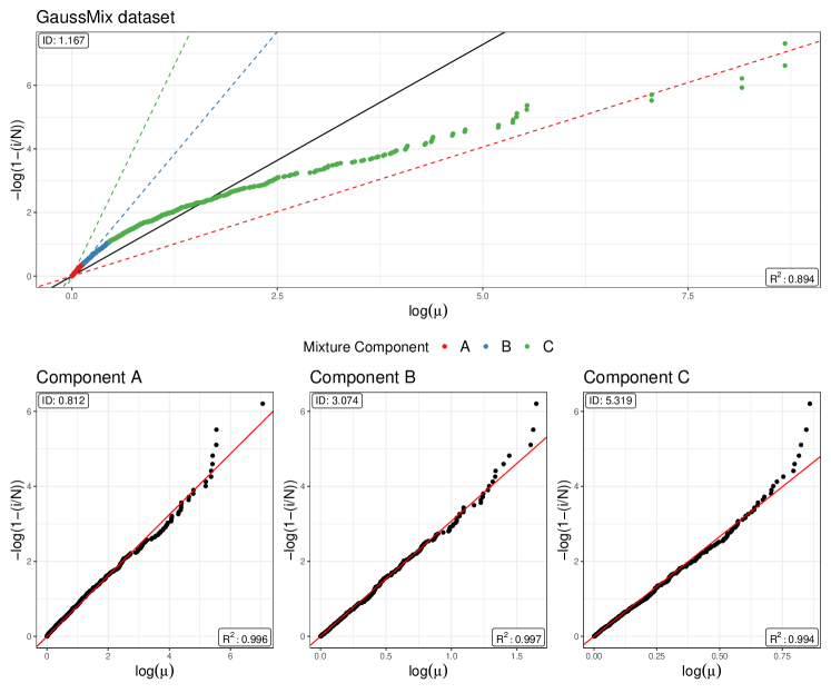
Figure 7: Linear estimators applied to the GaussMix dataset. In the top panel, the estimator is applied to the entire dataset. The points are colored according to the mixture component from which they originate, and the corresponding colored dashed lines result from applying the estimator to each known subset of points. The bottom three panels explicitly report the estimates within each mixture component.

We can get another empirical assessment by inspecting the evolution of the cumulative average distances between a point and its nearest neighbors. More formally, for each point $x_{i}$ we consider the evolution of the ergodic mean of the sorted sequence of distances $\left(r_{i,1},\ldots,r_{i,n}\right)$, given by $r_{i}(j)=\sum_{k=1}^{j}r_{i,k}/k,\>\forall i,j$. Figure 8 compares the Hypercube (left panel – exemplifying the homogeneous case) and GaussMix (right panel – representing the heterogeneous case) datasets. On the one hand, the left plot displays the ideal condition: there are no visible departures from the overall mean distance, which reassures us about the homogeneity assumption we made about the data. But, on the other hand, the right panel tells a different story. We immediately detect the different clusters in the data by focusing on their different starting values. The ergodic means remain approximately constant until the 500th NN, which corresponds to the size of each subgroup. The behavior of the cumulative means abruptly changes after the 500th NN, negating the presence of a unique manifold. This type of plot provides an empirical but valuable overview of the structure between data points, highlighting clusters that may reflect the existence of multiple manifolds.

These visual assessments help detect signs of the inappropriateness of the global ID assumption. The most direct approach to adopt in this case would be to divide the dataset into homogeneous subgroups and apply the TWO-NN estimator within each cluster. Such an approach is highlighted in the bottom panels of Figure 7. However, knowing ex-ante such well-separated groups is not a realistic expectation to have about actual data. Therefore, we will rely on Hidalgo(), the Bayesian finite mixture model for heterogeneous ID estimation described in Section 2.2.

Figure 8: Evolution of the cumulative means of NN distances computed for all the observations in the Hypercube (left panel) and GaussMix (right panel) datasets. In the right panel, the colors highlight the different mixture components.

3.4.2 Fitting the HIDALGO model

HIDALGO allows for the presence of multiple manifolds in the same dataset, yielding a vector of different estimated ID values. As already discussed, estimating a mixture model with Pareto components is challenging because of their extensive overlap. A naive model-based estimation can lead to inaccurate results since there is no clear separation between the kernel densities. The extra term $\prod_{i=1}^{n}\pi(\mathcal{N}_{i}^{(q)}|\bm{z})$ added into the likelihood in Equation 8 induces local homogeneity, which helps identify the model parameters.

The adjacency matrix $\mathcal{N}^{(q)}$ can be easily computed by specifying two additional arguments in the function compute_mus():

• Nq: logical, if TRUE, the function adds the adjacency matrix to the output;

• q: integer, the number of NNs to be considered in the construction of the matrix $\mathcal{N}^{(q)}$. The default value is 3.

To provide an idea of the structure of the adjacency matrix $\mathcal{N}^{(q)}$, we report three examples obtained from a random sub-sample of the GaussMix dataset for increasing values of q. We display the heatmaps of the resulting matrices in Figure 9.

R> set.seed(12345)
R> ind <- sort(sample(1:1500, 100, F))
R> Nq1 <- compute_mus(GaussMix[ind, ], Nq = T, q = 1)$NQ
R> Nq2 <- compute_mus(GaussMix[ind, ], Nq = T, q = 5)$NQ
R> Nq3 <- compute_mus(GaussMix[ind, ], Nq = T, q = 10)$NQ

As q increases, the binary matrix becomes more populated, uncovering the neighboring structure of the data points. Allegra et al. (2020) investigated how the performance of the model changes as q varies. They suggest fixing $\texttt{q}=3$, a value that provides a good trade-off between the flexibility of the mixture allocations and local homogeneity.

Figure 9: Heatmaps of the adjacency matrices $\mathcal{N}^{(q)}$ computed on a subset of observations of the GaussMix dataset. Different values of $q$ are assumed.

Given this premise, we are now ready to discuss Hidalgo(), the high-level function that fits the Bayesian mixture. It implements the Gibbs sampler described in Section C of the Appendix, relying on low-level Rcpp routines. Also, the function internally calls compute_mus() to automatically generate the ratios of distances and the adjacency matrix needed to evaluate the likelihood from the data points.

The function has the following arguments: X, dist_mat, q, D, and

• K: integer, number of mixture components;

• nsim, burn_in, and thinning: number of MCMC iterations to collect, initial iterations to discard, and thinning interval, respectively;

• verbose: logical, if TRUE, the progress of the sampler is printed;

• xi: real number between 0 and 1, a local homogeneity parameter. The default is 0.75;

• alpha_Dirichlet: hyperparameter of the Dirichlet prior on the mixture weights;

• a0_d and b0_d: shape and rate parameters of the Gamma prior on $d$. The default is 1 for both values;

• prior_type: string, type of Gamma prior on $d$ which can be

  • "Conjugate": a classic Gamma prior is adopted (default);

  • "Truncated": a truncated Gamma prior on the interval $\left(0,D\right)$ is used. This specification is advised when dealing with datasets characterized by a small number of columns, to avoid the estimated ID exceeding the nominal dimension D;

  • "Truncated_PointMass": same as Truncated, but a point mass is placed on $D$. That is, the estimated ID is allowed to be exactly equal to the nominal dimension D;

• pi_mass: probability placed a priori on $D$ when a Truncated_PointMass prior specification is chosen.

We apply the HIDALGO model on the GaussMix dataset with two different prior configurations: conjugate and truncated with point mass at $\texttt{D}=5$. The code we used to run the models is:

R> set.seed(1234)
R> hid_fit <- Hidalgo(X = GaussMix, K = 10,  alpha_Dirichlet = .05,
+                    nsim = 2000,   burn_in = 2000,  thinning = 5,
+                    verbose = FALSE)
R> set.seed(12345)
R> hid_fit_TR <- Hidalgo(X = GaussMix, K = 10, alpha_Dirichlet = .05,
+                       prior_type = "Truncated_PointMass", D = 5,
+                       nsim = 2000, burn_in = 2000, thinning = 5,
+                       verbose = FALSE)

We can print one of the returned objects to visualize a short summary of the run:

R> hid_fit_TR

Model: Hidalgo
Method: Bayesian Estimation
Prior d ~ Gamma(1, 1), type = Truncated_PointMass
Prior on mixture weights: Dirichlet(0.05) with 10 mixture components
MCMC details:
Total iterations: 4000, Burn in: 2000, Thinning: 5
Used iterations: 2000
Elapsed time: 2.2978 mins

By using alpha_Dirichlet = 0.05, we have adopted a sparse mixture modeling approach in the spirit of Malsiner-Walli et al. (2016). The sparse mixture approach would automatically let the data estimate the number of mixture components required. As a consequence, the argument K should be interpreted as an upper bound on the number of active clusters. Nonetheless, we stress that estimating the number of well-separated clusters with Pareto kernels is challenging. Hence, we will discuss how to analyze the output to perform proper inference. The output object hid_fit is a list of class Hidalgo, containing six elements:

• cluster_prob: matrix of dimension nsim$\times$K. Each column contains the MCMC sample of a mixing weight for every mixture component;

• membership_labels: matrix of dimension nsim$\times$n. Each column contains the MCMC sample of a membership label for every observation;

• id_raw: matrix of dimension nsim$\times$K. Each column contains the MCMC sample for the ID estimated in every cluster;

• id_postpr: matrix of dimension nsim$\times$n. It contains a chain for each observation, corrected for label-switching;

• id_summary: a matrix containing the posterior mean and the 5%, 25%, 50%, 75%, 95% quantiles for each observation;

• recap: a list with the specifications passed to the function as inputs.

To inspect the output, we can employ the dedicated autoplot() function devised for objects of class Hidalgo. There are several arguments that can be specified, producing different graphs. The most important is

• type: string that indicates the type of plot that is requested. It can be:

  • "raw_chains": plot the MCMC and the ergodic means not corrected for label-switching (default);

  • "point_estimates": plot the posterior mean and median ID for each observation, along with their CRIs;

  • "class_plot": plot the estimated ID distributions stratified by the groups specified in an additional class vector;

  • "clustering": plot the posterior co-clustering matrix. Rows and columns can be stratified by and exogenous class and/or a clustering structure.

For example, we can plot the raw chains of the two models with the aid of the patchwork package (Pedersen, 2020), producing Figure 10, via:

R> autoplot(hid_fit) / autoplot(hid_fit_TR)

Plotting the traceplots of the elements in $\bm{d}$ allows us to assess the convergence of the algorithm. First, however, we need to be aware that these chains may suffer from label-switching issues, preventing us from directly drawing inference from the MCMC output. Due to label-switching, mixture components can be discarded, emptied, or repopulated across iterations. This behavior is observed in Figure 10, which shows the MCMC traceplots of the two models, with the ergodic means for each mixture component superimposed. In this type of plot, we can often notice that various chains overlap around the prior mean of $d_{k}$. These chains represent the parameters of the empty clusters, which are sampled from the prior. For example, in the top panel of Figure 10 (Conjugate prior), $\mathbb{E}\left[d_{k}\right]=a_{d}/b_{d}=1$. Recall that the presence of empty clusters is favored by the sparse mixture setting.
Additionally, we can see that if no constraint is imposed on the support of the prior distribution for $\bm{d}$ (top panel), the posterior estimates can exceed the nominal dimension D = 5 of the GaussMix dataset. However, this problem disappears when imposing a truncation on the prior support (bottom panel).

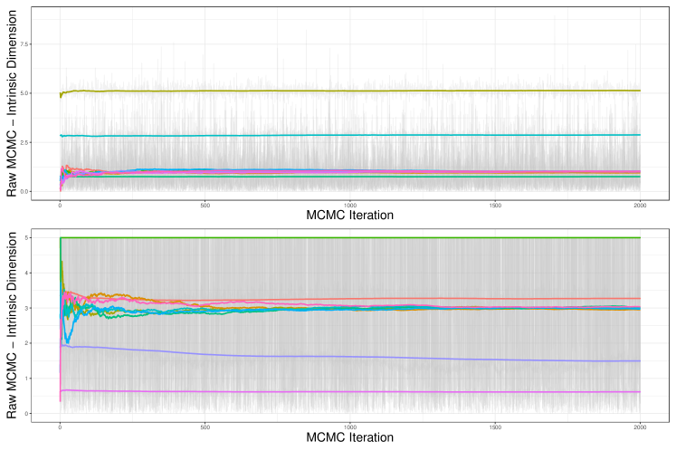
Figure 10: MCMC traceplots and superimposed ergodic means of the components of the ID vector. Top panel: conjugate prior specification. Bottom panel: truncated with point mass prior specification.

To address the label-switching issue and perform meaningful inference, the raw MCMC needs to be postprocessed. In Section D of the Appendix, we discuss the algorithm used to map the $K$ chains to $n$ observation-specific chains that can be employed for inference. The algorithm is already implemented in Hidalgo(), and produces the elements id_postpr and id_summary in the returned list. We can obtain a visual summary of the postprocessed estimates via

R> autoplot(hid_fit, type = "point_estimates") +
+  autoplot(hid_fit_TR, type = "point_estimates")

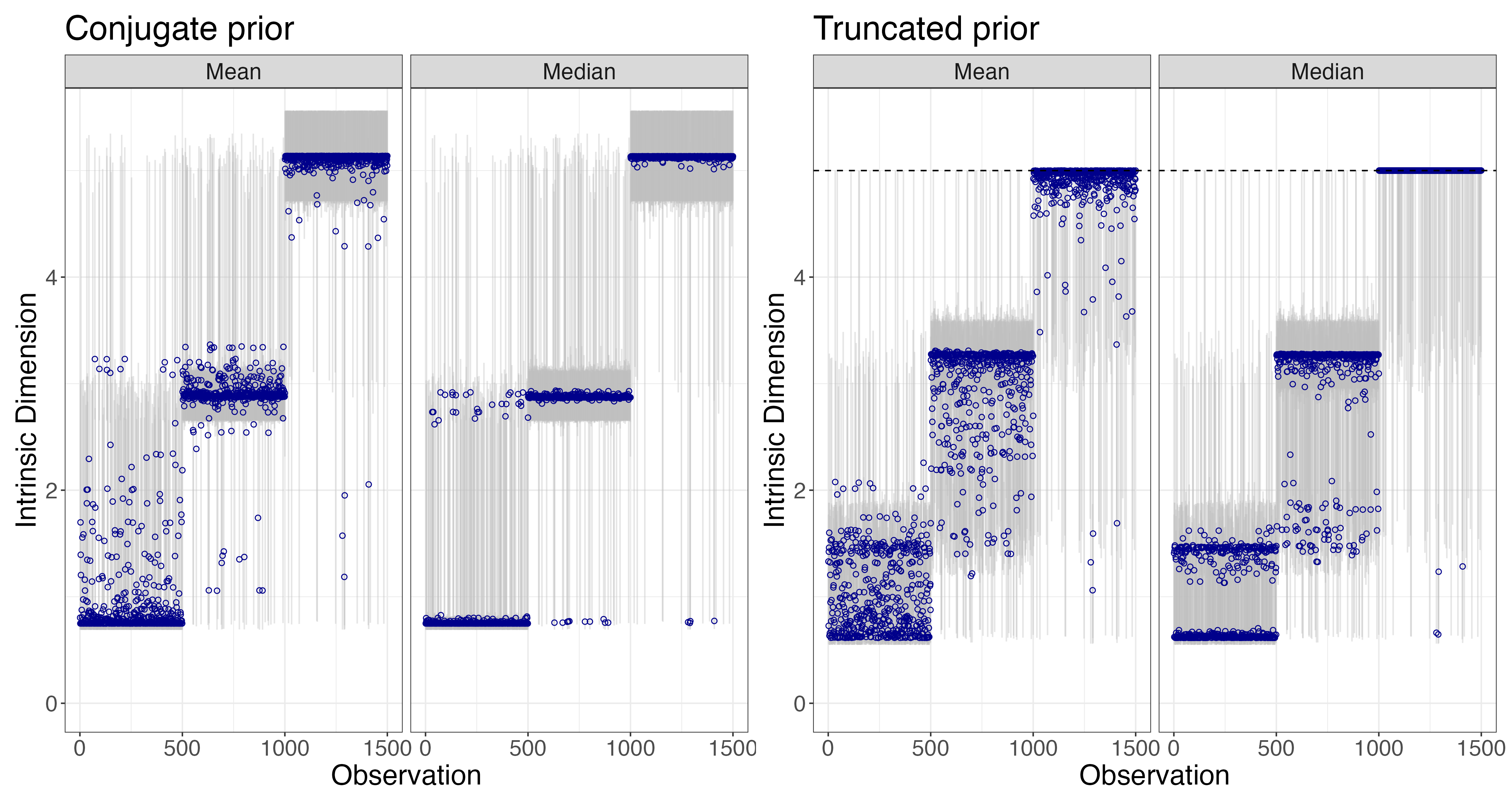
Figure 11: Observation-specific posterior means (left panels) and medians (right panels) ID represented with blue dots. The gray bars represent the $90\%$ CRIs. The two plots correspond to two different prior specifications.

The resulting plots are shown in Figure 11. The panels display the mean and median ID estimates for each data point. Here, the separation of the data into different generating manifolds is evident. Also, we notice that some of the estimates in the conjugate case are incorrectly above the nominal value D = 5, once again justifying the need for a truncated prior. The default plots were modified with coord_cartesian(ylim = c(0, 5.5)) to highlight the effect of the truncation.

3.4.3 Estimated clustering solutions

It is natural to seek model-based clustering solutions when dealing with a mixture model. To this extent, the key source of information is the posterior similarity – or co-clustering – matrix (PSM). The entries $\{s_{i,j}\}_{i,j=1}^{n}$ of this matrix are computed as the proportion of times in which two observations have been assigned to the same mixture component across the MCMC iterations. Thus, the PSM describes the underlying clustering structure of the data detected by HIDALGO. Given the PSM, one can evaluate various loss functions on the space of the partitions. By minimizing the loss functions, we can retrieve the optimal partition of the dataset into clusters. To obtain such estimate, we rely on the function salso() from the R packages salso (Dahl et al., 2021). Otherwise, a faster alternative method proceeds by building a dendrogram from the implied posterior dissimilarity matrix (PDM), whose entries are given by $\{d_{i,j}\}_{i,j=1}^{n}$ where $d_{i,j}=1-s_{i,j}$, $\forall i,j$. Once the dendrogram is built, we can threshold it to segment the data into a pre-specified number of clusters K.

These approaches are implemented in the dedicated function clustering() which takes as arguments, along the object output from the Hidalgo() function,

• clustering_method: string indicating the method to use to perform clustering. It can be "dendrogram" or "salso". The former method thresholds the dendrogram constructed from the PDM to retrieve exactly K clusters. The latter method estimates the optimal clustering solution by minimizing a loss function on the space of the partitions. The default loss function is the variation of information (VI, Wade and Ghahramani, 2018). For additional details about the VI loss function, see Section E of the Appendix;

• K: integer, used when "dendrogram" is chosen. It corresponds to the number of clusters to recover when thresholding the dendrogram obtained from the PDM;

• nCores: integer, argument used in the functions called from salso. It represents the number of cores used to compute the PSM and the optimal clustering solution.

Additional arguments can be passed to personalize the partition estimation via salso(). Given the large sample size of the GaussMix dataset, we opt for the dendrogram approach, truncating the dendrogram at K = 3 groups. We highlight that relying on the minimization of a loss function is a more principled approach. However, the method can be misled by the strongly overlapping clusters estimated across the MCMC iterations, providing overly conservative solutions.

R> psm_cl <- clustering(object = hid_fit_TR,
+                      clustering_method = "dendrogram",
+                      K=3, nCores = 5)
R> psm_cl

Estimated clustering solution summary:

Method: dendrogram
Retrieved clusters: 3
Clustering frequencies:

| Cluster 1| Cluster 2| Cluster 3|
|---------:|---------:|---------:|
|       554|       450|       496|

To visualize the results, we can also plot the PSM by passing an object of class Hidalgo to autoplot() with type = "clustering". autoplot() internally calls the function clustering() to compute the PSM. One can also specify an additional argument class to stratify the observations according to exogenous factors.

3.4.4 The presence of patterns in the data uncovered by the ID

Once the observation-specific estimates are computed, we can investigate the presence of potential patterns between the recovered IDs and given exogenous variables. To explore these possible relations, we can use the function id_by_class(). Along with an object of class Hidalgo, we need to specify:

• class: factor, a variable used to stratify the ID posterior estimates.

For the GaussMix dataset, the exogenous information is contained in the class_GMix vector, which we pass as class.

R> id_by_class(object = hid_fit_TR, class = class_GMix)

Posterior ID by class:

|class |     mean|    median|        sd|
|:-----|--------:|---------:|---------:|
|A     | 1.031105| 0.9019793| 0.3781802|
|B     | 2.961009| 3.2068593| 0.4683262|
|C     | 4.864018| 4.9685900| 0.3774186|

The estimates in the three classes are very close to the ground truth. The same argument, class, can be passed to the autoplot() function, in combination with

• class_plot_type: string, if type = "class_plot", one can visualize the stratified ID estimates with a "density" plot or a "histogram", or using "boxplots" or "violin" plots;

• class: a vector containing a class used to stratify the observations;

to visualize ID estimates of the GaussMix dataset stratified by the generating manifold of the observations. As an example of possible graphs, Figure 12 shows the stratified boxplots (left panel) and histograms (right panel).

R> autoplot(hid_fit_TR, type = "class", class = class_GMix,
+          class_plot_type = "boxplot") +
+ autoplot(hid_fit_TR, type = "class", class = class_GMix,
+           class_plot_type = "histogram")

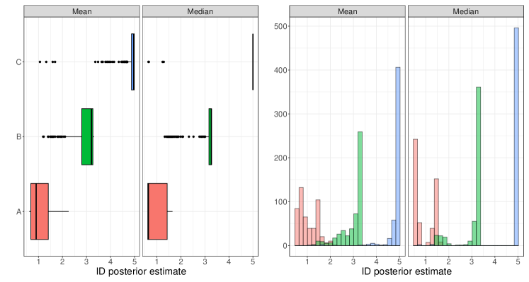
Figure 12: Two different types of graphs used to stratify the estimated IDs by a given exogenous variable.

We have introduced and discussed the principal functions of the intRinsic package concerning the TWO-NN and HIDALGO models. Then, by employing simulated data with known IDs, we have suggested a pipeline to guide our study. In the next section, we present a real data analysis, highlighting how the ID estimation can be used to effectively reduce the size of a dataset while capturing and preserving important features.

4 The ID of gene microarray measurements

In this section, we present a real data example investigating the ID of the Alon dataset. The dataset, first presented in Alon et al. (1999), contains microarray measurements for 2000 genes measured on 62 patients. Among the patients, 40 were diagnosed with colon cancer, and 22 were healthy subjects. A factor variable named status describes the patient health condition (coded as "Cancer" vs. "Healthy"). A copy of this famous dataset can be found in the R package HiDimDA (Silva, 2015). We store the gene measurements in the object Xalon, a matrix of nominal dimension D = 2000, with n = 62 observations. To load and prepare the data, we write:

R> data("AlonDS", package = "HiDimDA")
R> status <- factor(AlonDS$grouping, labels = c("Cancer", "Healthy"))
R> Xalon  <- as.matrix(AlonDS[, -1])

To obtain a visual summary of the dataset, we plot the heatmap of the log-data values annotated by status. The result is shown in Figure 13. No clear structure is immediately visible.

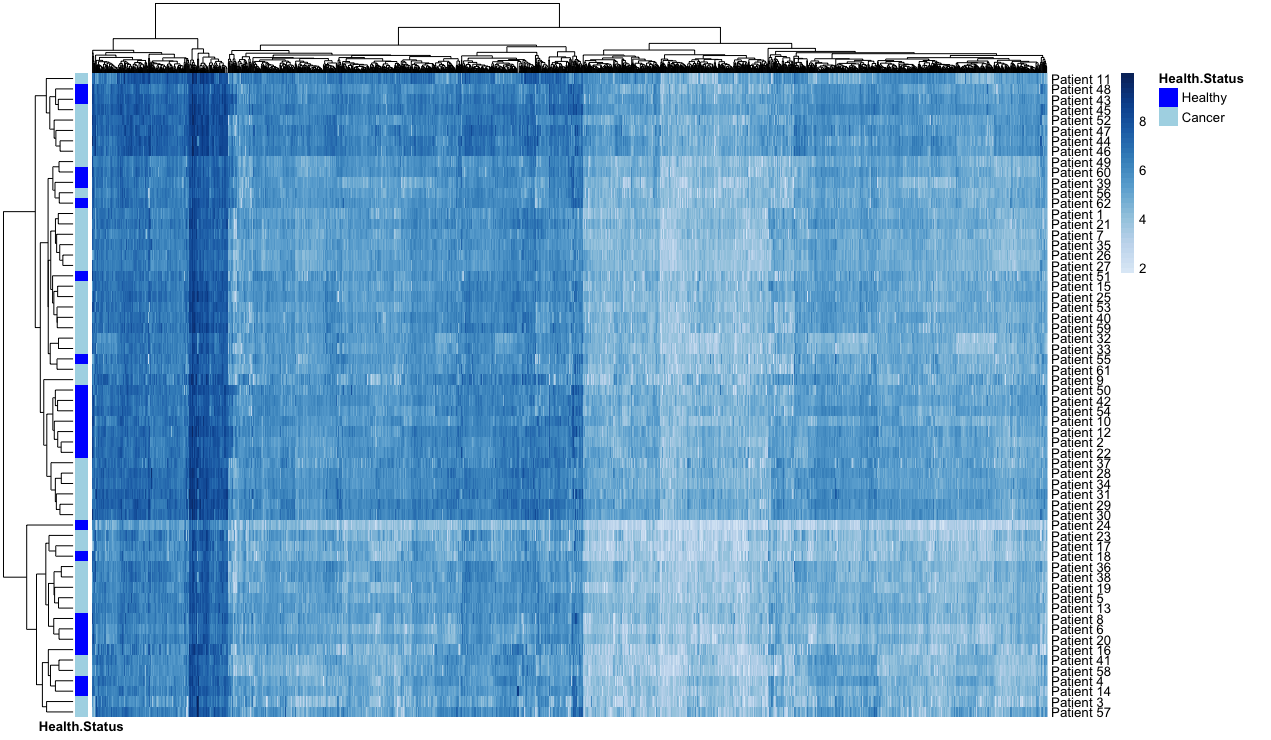
Figure 13: Heatmap of the log-values of the Alon microarray dataset. The patients on the rows are labeled according to their health status.

We ultimately seek to uncover hidden patterns in this dataset. The task is challenging, especially given the small number of available observations. As a first step, we investigate how well a unique, global ID estimate can represent the data.

4.1 Homogeneous ID estimation

Let us start by describing the overall complexity of the dataset by estimating a homogeneous ID value. Using the TWO-NN model, we can compute:

R> Alon_twonn_1 <- twonn(Xalon,method = "linfit")
R> summary(Alon_twonn_1)

Model: TWO-NN
Method: Least Squares Estimation
Sample size: 62, Obs. used: 61. Trimming proportion: 1%
ID estimates (confidence level: 0.95)

| Lower Bound| Estimate| Upper Bound|
|-----------:|--------:|-----------:|
|    10.00382| 10.34944|    10.69506|

R> Alon_twonn_2 <- twonn(Xalon,method = "bayes")
R> summary(Alon_twonn_2)

Model: TWO-NN
Method: Bayesian Estimation
Sample size: 62, Obs. used: 61. Trimming proportion: 1%
Prior d ~ Gamma(0.001, 0.001)
Credibile Interval quantiles: 2.5%, 97.5%
Posterior ID estimates:

| Lower Bound|     Mean|   Median|     Mode| Upper Bound|
|-----------:|--------:|--------:|--------:|-----------:|
|    7.784152| 10.17639| 10.12084| 10.00957|    12.88427|

R> Alon_twonn_3 <- twonn(Xalon,method = "mle")
R> summary(Alon_twonn_3)

Model: TWO-NN
Method: MLE
Sample size: 62, Obs. used: 61. Trimming proportion: 1%
ID estimates (confidence level: 0.95)

| Lower Bound| Estimate| Upper Bound|
|-----------:|--------:|-----------:|
|    7.785304| 10.01107|    12.88623|

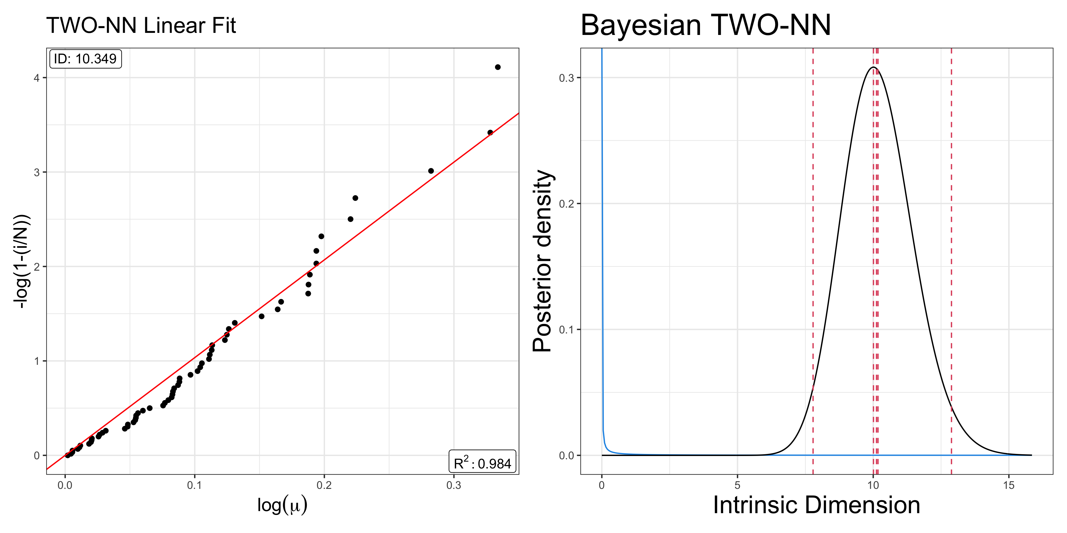
Figure 14: Alon dataset. The left panel shows the result of the linear estimator, while the right panel depicts the posterior distribution obtained via the Bayesian approach.

The estimates based on the TWO-NN model obtained with different methods are very similar. The results are also illustrated in Figure 14, which shows the linear fit (left panel) and posterior distribution (right panel) for the TWO-NN model. According to these results, we conclude that the information contained in the D = 2000 genes can be summarized with approximately ten variables. For example, the first ten eigenvalues computed from the spectral decomposition of the matrix $\Lambda=X_{Alon}^{{}^{\prime}}X^{\>}_{Alon}$ contribute to explaining the 95.4% of the total variance.

Although the linear fit plot and the TWO-NN estimates do not raise any evident sign of concern, as a final check, we explore the evolution of the average distances between NN, reported in Figure 15. As expected, the plot does not highlight any abrupt change in the evolution of the ergodic means. However, it suggests that investigating the presence of multiple manifolds could be interesting. In fact, despite the evolution of most of the ergodic means being stationary, their heterogeneous levels highlight some potential data inhomogeneities that should be deepened.

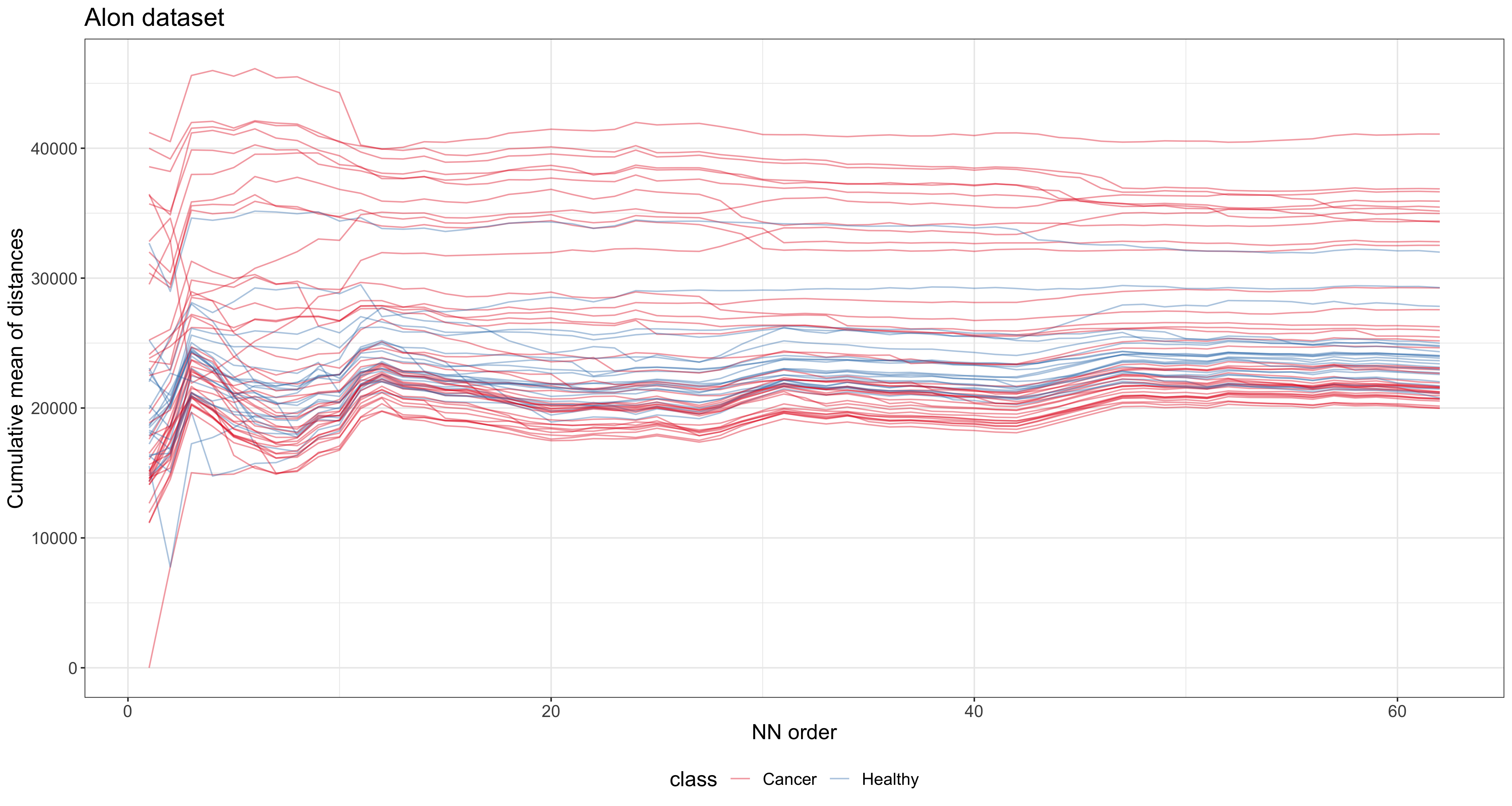
Figure 15: Evolution of the cumulative means of NN distances computed for all the observations in the Alon dataset.

4.2 Heterogeneous ID estimation

To investigate the presence of heterogeneous latent manifolds in the Alon dataset, we employ Hidalgo(). Since the nominal dimension D is large, we do not need to truncate the prior on $d$. Moreover, given the small number of data points, we opt for an informative and regularizing prior $Gamma(1,1)$ (the default) instead of a vague specification. Also, we set a conservative upper bound for the mixing component K = 15 and choose again $\alpha=0.05$ to fit a sparse mixture. We run:

R> set.seed(1234)
R> Alon_hid <- Hidalgo(X = Xalon,  K = 15, a0_d = 1, b0_d = 1,
+             alpha_Dirichlet = .05,
+             nsim = 10000, burn_in = 100000, thin = 5)

R> Alon_hid

Model: Hidalgo
Method: Bayesian Estimation
Prior d ~ Gamma(1, 1), type = Conjugate
Prior on mixture weights: Dirichlet(0.05) with 15 mixture components
MCMC details:
Total iterations: 110000, Burn in: 1e+05, Thinning: 5
Used iterations: 10000
Elapsed time: 38.3067 secs

Once the model is fitted, we first explore the estimated clustering structure. Here, instead of directly plotting the heatmap of the PSM, we build the dendrogram from the PDM, and we report it in the top panel of Figure 16. We construct such a plot with the help of the package ggdendro (de Vries and Ripley, 2020). We can detect four clusters, and therefore we decide to set K = 4 when running

R> Alon_psm <- clustering(Alon_hid, K = 4)

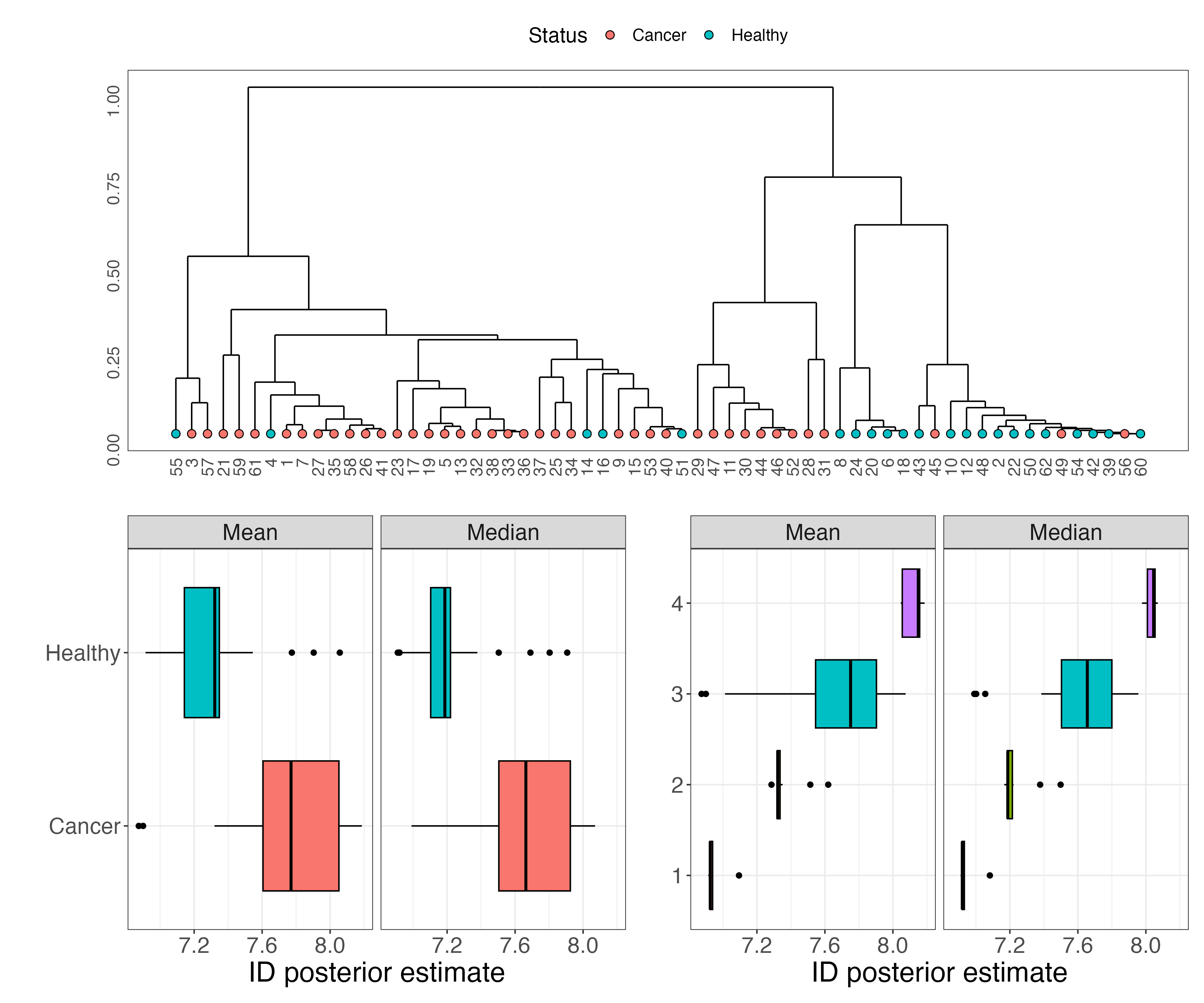
Figure 16: Alon dataset. Top panel: dendrogram obtained from the PDM. Bottom panel: boxplots of the ID estimates stratified by health status (left) and estimated partition (right).

As illustrated in the previous section, all these plots can be obtained by calling autoplot() with the proper argument specifications. The next natural step is to investigate how strongly the estimated partition and, in general, the estimated IDs are associated with health status. The bottom two panels of Figure 16 display the boxplots of the values (means and medians) of the postprocessed, observation-specific IDs stratified by status (left) and estimated cluster (right). We can also run

R> id_by_class(Alon_hid,class = status)
R> id_by_class(Alon_hid,class = Alon_psm$clust)

to obtain summary results linking the variations in the ID with health status and cluster. We report the output in Table 6. As the estimated ID increases, the proportion of healthy subjects in each cluster decreases. This result suggests that the microarray profiles of people diagnosed with cancer are slightly more complex than healthy patients’ ones.

Cluster	# Cancer	# Healthy	% Healthy	Average ID	Median ID	Std. Dev.
1	0	5	1.0000	6.9595	6.9252	0.0761
2	3	12	0.8000	7.3564	7.3222	0.0889
3	28	5	0.1515	7.6883	7.7513	0.3083
4	9	0	0.0000	8.1198	8.1493	0.0546

Table 6: Stratification by cluster of the health status (frequencies and proportions of healthy patients) and ID estimates (mean, median, and standard deviation).

The analyses conducted so far helped us uncover interesting descriptive characteristics of the IDs in the dataset. Nevertheless, these results can also be effectively used as a representative data summary. Here, we show how the estimated individual IDs are valid to potentially classify the health status of new patients according to their genomic profiles. As a simple example, we perform a classification analysis using two random forest models, predicting the target variable Y = status. To train the models, we use two different sets of covariates: X_OR, the original dataset composed of 2000 genes,

R> X_OR <- data.frame(Y = status, X = Xalon)
R> set.seed(1231)
R> rfm1 <- randomForest::randomForest(Y ~ ., data = X_OR,
+                                    type = "classification", ntree=100)

and X_ID, the observation-specific ID summary returned by Hidalgo(), along with our estimated partition.

R> X_ID <- data.frame(Y     = status,
+                    X     = summary(Alon_hid),
+                    clust = factor(Alon_psm$clust))
R> set.seed(1231)
R> rfm2 <- randomForest::randomForest(Y ~ ., data = X_ID,
+                                    type = "classification", ntree=100)

The classification results are reported in Table 7.

rfm1	Cancer	Healthy	class.err	rfm2	Cancer	Healthy	class.err
Cancer	36	4	0.100	Cancer	35	5	0.1250
Healthy	9	13	0.409	Healthy	6	16	0.273
Dataset:	X_OR	OOB err:	20.97%	Dataset:	X_ID	OOB err:	17.74%

Table 7: Confusion matrices summarizing the classification performance of the two random forest models, trained with the orginal gene expressions (rfm1, left) and with a summary of the ID estimates (rfm2, right).

Remarkably, a simple dataset with seven variables summarizing the main distributional traits of the observation-specific posterior IDs obtains good performance in predicting health status, similar to the original dataset. More precisely, the random forest on the original dataset got an out-of-bag estimated error rate of 20.97%, while the error is reduced to 17.74% when using our ID-based covariates. We can conclude that, in this case, the topological properties of the dataset are associated with the outcome of interest and convey important information.

We showed how the estimation of heterogeneous ID provides a reliable complexity index for elaborate data structures and helps unveil relationships among data points hidden at the topological level. The application to the Alon dataset showcases how reliable ID estimates give additional fundamental perspectives that help us discover non-trivial data patterns. Furthermore, one can exploit the extracted information in many downstream investigations, such as patient segmentation or predictive analyses.

5 Summary and discussion

In this paper, we illustrated intRinsic, an R package that implements novel routines for the ID estimation according to the models recently developed in Facco et al. (2017); Allegra et al. (2020); Denti et al. (2022), and Santos-Fernandez et al. (2022). intRinsic consists of a collection of high-level, user-friendly functions that, in turn, rely on efficient, low-level routines implemented in R and C++. We also remark that intRinsic integrates functionalities from external packages. For example, all the graphical outputs returned by the functions are built using the well-known package ggplot2. Therefore, they are easily customizable using the grammar of graphics (Wilkinson, 2005).

The package includes frequentist and Bayesian model specifications for the TWO-NN global ID estimator. Moreover, it implements the Gibbs sampler for posterior simulation of the HIDALGO model, which can capture the presence of heterogeneous ID within a single dataset. We showed how discovering multiple latent manifolds could help unveil the topological traits of a dataset, primarily when additional exogenous variables are used to stratify the ID estimates.

As a general analysis pipeline for practitioners, we suggested starting with the efficient TWO-NN functions to understand how appropriate the hypothesis of homogeneity is for the data at hand. If departures from the assumptions are visible from nonuniform estimates obtained with different estimation methods and from visual assessment of the evolution of the average NN distances, one should rely on HIDALGO.

The most promising future research directions stem from HIDALGO. First, we plan to develop more reliable methods to obtain an optimal partition of the data based on the ID estimates since the one proposed heavily relies on a mixture model of overlapping distribution. Moreover, another research avenue worth exploring is a version of HIDALGO with likelihood distributions based on generalized NN ratios, exploiting the information coming from varying neighborhood sizes.
We also know that the mixture model fitting may become computationally expensive if the analyzed datasets are large. Therefore, faster solutions, such as the Variational Bayes approach, will be explored. Also, we highlight that HIDALGO, a mixture model within a Bayesian framework, lacks a frequentist-based estimation counterpart, such as an Expectation Maximization algorithm. Its derivation is not immediate since the neighboring structure introduced via the $\mathcal{N}^{(q)}$ matrix makes the problem non-trivial. We plan to keep working on this package and continuously update it in the long run as contributions to this line of research become available. The novel ID estimators we discussed have started a lively research branch, and we intend to include all the future advancements in intRinsic.

Appendix

A - Additional methods implemented in the package

In this paper, we have focused our attention on the TWO-NN and the HIDALGO models. In Section 2, we explained that both methods are based on the distributional properties of the ratios of distances between a point and its first two NNs. However, this modeling framework has been extended by Denti et al. (2022), where the authors developed a novel ID estimator called GRIDE. This new estimator is based upon the ratios of distances between a point two of its NNs of generic order, namely $n_{1}$ and $n_{2}$. Extending the neighborhood size leads to two major implications: more stringent local homogeneity assumptions and the possibility of computing ID estimates as a function of the chosen NN orders. Monitoring the ID evolution as the order of the furthest NN $n_{2}$ increases allows the extraction of meaningful information regarding the link between the ID and the scale of the considered neighborhood. In doing so, GRIDE produces estimates that are more robust to noise present in the data, which is not directly addressed by the model formulation.

The GRIDE model is implemented in intRinsic, and the estimation can be carried out under both the frequentist and Bayesian frameworks via the function gride(), which is very similar to twonn() in its usage. Additionally, one can use the functions twonn_decimation() and gride_evolution() to study the ID dynamics. More details about these functions are available in the package documentation.

The map in Figure 17 provides a visual summary of the most important functions contained in the package. The main topics are reported in the diamonds, while the high-level, exported functions are displayed in the blue rectangles. These routines are linked to the (principal) low-level function via dotted lines. Finally, the light-blue area highlights the functions discussed in this paper.

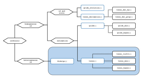
Figure 17: A conceptual map summarizing the most important functions contained in intRinsic. The blue squares contain the names of the principal, high-level functions. Dotted lines connect these functions with the most important low-level functions (not exported). The light-blue area represents the topics that have been discussed in this paper.

B - intRinsic and other packages

As mentioned in Section 1, there is a large number of ID estimators available in the literature, and many of them have been implemented in R. A valuable survey of the availability of dimensionality reduction methods and ID estimators has been recently reported in You (2020a). From there, we see that two packages are the most important when it comes to ID estimation: Rdimtools and intrinsicDimension. Rdimtools, in particular, is comprised of an unprecedented collection of methods – including also the least-squares TWO-NN.
At the moment of writing, two main traits of intRinsic are unique to this package.
First, our package is devoted to the recently proposed likelihood-based estimation methods introduced by the seminal work of Facco et al. (2017) and the literature that followed. Therefore, as of today, many of the R implementations presented here are exclusively contained in this package. This is true, for example, for the MLE and Bayesian versions of the TWO-NN model, the HIDALGO model, and all the routines linked to GRIDE. To the best of our knowledge, the function Hidalgo() is available outside this package. However, one can only find it on GitHub repositories, coded in Python and C++. Note that Python versions of the TWO-NN estimator have also been implemented in the recent scikit-dimension and DADApy packages (Bac et al., 2021; Glielmo et al., 2022). Moreover, DADApy contains routines dedicated to GRIDE. Table 8 presents a summary of recent software packages containing ensembles of ID estimation methods.
Second, all the functions in our package allow – and emphasize – the uncertainty quantification around the ID estimates, which is a crucial component granted by our model-based approach. This feature is often overlooked in other implementations.

Package	Language	ID estimation methods	Overlap with intrRinsic
intrinsicDimension	R	5	–
Rdimtools	R	17	TWO-NN§
ider	R	7	–
DADApy	Python	2	TWO-NN†,‡,§, GRIDE†
scikit-dimension	Python	19	TWO-NN§

Table 8: A non-exhaustive list of the most recent software packages for ID estimation in R and Python. The superscripts indicate the implemented estimation procedures. In detail: ^†MLE; ^‡Bayesian estimation; ^§linear fit.

Overall, the wide variety of methods and ongoing research in this area indicate that there is no globally optimal estimator to employ regardless of the application. Thus, a practitioner should be aware of the strengths and limitations of every method.
One limitation of the likelihood-based models offered in this package, shared with many other ID estimators in general, is the underestimation of the ID when the true latent manifold’s dimension is large. As an empirical rule, for cases where the estimated ID is large (e.g., $d>20$), the retrieved value should be cautiously regarded as a lower bound for the actual ID (Ansuini et al., 2019). An alternative method we found particularly robust to this issue is the Expected Simplex Skewness (ESS) algorithm proposed by Johnsson et al. (2015). For example, consider 5000 observations sampled from a $D=d=50$ dimensional Gaussian distribution. With the following code, we can see how twonn() underestimates the true ID, which the ESS instead recovers well.

R> set.seed(12211221)
R> X_highdim <- replicate(50, rnorm(5000))
R> intrinsicDimension::essLocalDimEst(X_highdim)

Dimension estimate: 49.05083
Additional data: ess

R> summary(twonn(X_highdim))

Model: TWO-NN
Method: MLE
Sample size: 5000, Obs. used: 4950. Trimming proportion: 1%
ID estimates (confidence level: 0.95)

| Lower Bound| Estimate| Upper Bound|
|-----------:|--------:|-----------:|
|    34.92154| 35.90791|    36.92254|

However, the ESS is not uniformly optimal. For example, for the Swissroll data, the twonn() performs better:

R> intrinsicDimension::essLocalDimEst(Swissroll)

Dimension estimate: 2.898866
Additional data: ess

R> summary(twonn(Swissroll, c_trimmed = .001))

Model: TWO-NN
Method: MLE
Sample size: 1000, Obs. used: 999. Trimming proportion: 0.1%
ID estimates (confidence level: 0.95)

| Lower Bound| Estimate| Upper Bound|
|-----------:|--------:|-----------:|
|    1.945607|  2.07005|    2.202571|

When dealing with a dataset characterized by many columns, we suggest checking the discrepancy between our methods and different competitors. A marked difference in the results should flag the likelihood-based findings as less reliable. At this point, a legitimate doubt that may arise regards the validity of the findings we obtained studying the Alon dataset. Because of its high number of columns (D = 2000), the ID we recovered may have been strongly underestimated. To validate our results, we run the ESS estimator on the Alon dataset, obtaining

R> intrinsicDimension::essLocalDimEst(data = Xalon)

Dimension estimate: 7.752803
Additional data: ess

which is very close to the estimates obtained with our methods, reassuring us about our conclusions.

C - Gibbs sampler for Hidalgo()

The steps of the Gibbs sampler are the following:

1. Sample the mixture weights according to

   $$\bm{\pi}|\cdots\sim Dirichlet\left(\alpha_{1}+\sum_{i=1}^{n}\mathds{1}_{z_{i}=1},\ldots,\alpha_{K}+\sum_{i=1}^{n}\mathds{1}_{z_{i}=K}\right)$$

2. Let $\bm{z}_{-i}$ denote the vector $\bm{z}$ without its $i$-th element. Sample the cluster indicators $z_{i}$ according to:

   $$\mathbb{P}\left(z_{i}=k|\bm{z}_{-i},\cdots\right)\propto\pi_{z_{i}}f\left(\mu_{i},\mathcal{N}_{i}^{(q)}|z_{1},\ldots,z_{i-1},k,z_{i+1},\ldots,z_{n},\bm{d}\right)$$

   We emphasize that, given the new likelihood we are considering, the cluster labels are no longer independent given all the other parameters. Let us define

   $$\bm{z}_{i}^{k}=\left(z_{1},\ldots,z_{i-1},k,z_{i-1},\ldots,z_{n}\right).$$

   Then, let $N_{z_{i}}(\bm{z}_{-i})$ be the number of elements in the $(n-1)$-dimensional vector $\bm{z}_{-i}$ that are assigned to the same manifold (mixture component) as $z_{i}$. Moreover, let $m_{i}^{in}=\sum_{l}\mathcal{N}_{li}^{(q)}\mathds{1}_{z_{l}=z_{i}}$ be the number of points sampled from the same manifold of the $i$-th observation that have ${x}_{i}$ as neighbor, and let $n_{i}^{in}(\bm{z})=\sum_{l}\mathcal{N}_{il}^{(q)}\mathds{1}_{z_{l}=z_{i}}\leq q$ be the number of neighbors of ${x}_{i}$ sampled from the same manifold. Then, we can simplify the previous formula, obtaining the following full conditional:

   $$\mathbb{P}\left(z_{i}=k|\bm{z}_{-i},\cdots\right)\propto \frac{\pi_{k}d_{k}\mu_{i}^{-(d_{k}+1)}}{\mathcal{Z}\left(\zeta,N_{z_{i}=k}(\bm{z}_{-i})+1\right)}\times\left(\frac{\zeta}{1-\zeta}\right)^{n_{i}^{in}(\bm{z}_{i}^{k})+m_{i}^{in}(\bm{z}_{i}^{k})}$$ (10)

   $$\times \left(\frac{\mathcal{Z}\left(\zeta,N_{z_{i}=k}(\bm{z}_{-i})\right)}{\mathcal{Z}\left(\zeta,N_{z_{i}=k}(\bm{z}_{-i})+1\right)}\right)^{N_{z_{i}=k}(\bm{z}_{-i})}.$$

   See Facco and Laio (2017) for a detailed derivation of this result.

3. The posterior distribution for $\bm{d}$ depends on the prior specification we adopt:

   1. If we assume a conjugate Gamma prior, we obtain

      $$d_{k}|\cdots\sim Gamma\left(a_{0}+n_{k},b_{0}+\sum_{i:z_{i}=k}\log\mu_{i}\right),$$

      where $n_{k}=\sum_{i=1}^{n}\mathds{1}_{z_{i}=k}$ is the number of observations assigned to the $k$-th group;
      

   2. If $G_{0}$ is assumed to be a truncated Gamma distribution on $\left(0,D\right)$, then

      $$d_{k}|\cdots\sim Gamma\left(a_{0}+n_{k},b_{0}+\sum_{i:z_{i}=k}\log\mu_{i}\right)\mathds{1}(\cdot)_{\left(0,D\right)};$$

   3. Finally, let us define $a^{*}=a_{0}+n_{k}$ and $b^{*}=b_{0}+\sum_{i:z_{i}=k}\log\mu_{i}$, if $G_{0}$ is assumed to be a truncated Gamma with point mass at $D$ we obtain

      $$d_{k}|\cdots\sim\frac{\hat{\rho}_{1}^{*}}{\hat{\rho}_{1}^{*}+\hat{\rho}_{0}^{*}}\>Gamma\left(a^{*},b^{*}\right)\mathds{1}(\cdot)_{\left(0,D\right)}+\frac{\hat{\rho}_{0}^{*}}{\hat{\rho}_{1}^{*}+\hat{\rho}_{0}^{*}}\>\delta_{D}(\cdot),$$

      where $\hat{\rho}_{1}^{*}=\hat{\rho}\cdot(\mathcal{C}_{a^{*},b^{*},D}/\mathcal{C}_{a,b,D})$ and $\hat{\rho}_{0}^{*}=(1-\hat{\rho})\cdot D^{n_{k}}\cdot\exp\{-D\sum_{i:z_{i}=k}\log\mu_{i}\}$.

D - Postprocessing to address label-switching

The postprocessing procedure adopted for the raw chains fitted by Hidalgo() works as follows.

Recall that we are working with $n$ observations and $K$ mixture components. Let us consider an MCMC sample of length $T$, and denote a particular MCMC iteration with $t$, $t=1,\ldots,T$. Let $z_{i}{(t)}$ indicate the cluster membership of observation $i$ at the $t$-th iteration, with $i=1,\ldots,n$. Similarly, $d_{k}{(t)}$ represents the value of the estimated ID in the $k$-th mixture component at the $t$-th iteration, where $k=1,\ldots,K$.
We map the $K$ chains of the parameters in $\bm{d}$ to each data point via the values of $\bm{z}$. That is, we construct $n$ chains, one for each observation. At the $t$-th iteration, we will have $\{d_{z_{i}{(t)}}{(t)}\}_{i=1}^{n}$. In so doing, we obtain a collection of $n$ chains that link every observation to its ID estimate. When the chains have been postprocessed, the local observation-specific ID can be estimated by the ergodic mean or median.

E - The variation of information metric

This section provides additional details regarding the variation of information (VI) distance between partitions, a quantity often employed to estimate optimal posterior clustering configurations.

First, let $|A|$ denote the cardinality of a generic set $A$. Then, consider two different partitions of $n$ elements defined as $\rho_{1}=\{S^{1}_{1}\ldots,S^{1}_{p_{1}}\}$ and ${\rho_{2}}=\{S^{2}_{1}\ldots,S^{2}_{p_{2}}\}$. By definition, for $q=1,2$, we have that $S^{q}_{i}\cap S^{q}_{j}=\varnothing$ when $i\neq j$, that $|\rho_{1}|=p_{1}$, $|\rho_{2}|=p_{2}$, and that $\sum_{l=1}^{p_{q}}|S^{q}_{l}|=n$. Following the notation in Dahl et al. (2022), we define the individual entropy function as $H(\rho_{q})=-\sum_{S\in\rho_{q}}|S|/n\log_{2}\left(|S|/n\right)$ for $q=1,2$. Moreover, the joint entropy $H(\rho_{1},\rho_{2})$ and mutual information $I(\rho_{1},\rho_{2})$ are defined as

$$H(\rho_{1},{\rho_{2}}) =-\sum_{S^{1}\in\rho_{1}}\sum_{S^{2}\in{\rho_{2}}}\frac{|S^{1}\cap S^{2}|}{n}\log_{2}\left(\frac{|S^{1}\cap S^{2}|}{n}\right),$$

$$I(\rho_{1},{\rho_{2}}) =H(\rho_{1})+H({\rho_{2}})-H(\rho_{1},{\rho_{2}}).$$

Given these quantities, Meila, Marina (2007); Vinh et al. (2010) considered the variation of information as a distance between partitions:

$$\mathcal{L}_{VI}(\rho_{1},\rho_{2})=H(\rho_{1})+H(\rho_{2})-2I(\rho_{1},\rho_{2})=-H(\rho_{1})-H(\rho_{2})+2H(\rho_{1},\rho_{2}).$$ (11)

Wade and Ghahramani (2018) used Equation 11 as a loss function to measure the discrepancy between the targeted posterior partition $\rho_{1}=\rho$ and an estimated one $\rho_{2}=\hat{\rho}$. By minimizing the posterior expectation of $\mathcal{L}_{VI}(\rho,\hat{\rho})$ w.r.t. $\hat{\rho}$, one obtains the optimal clustering solution:

$$\hat{\rho}^{*}=\arg\min_{\hat{\rho}}\mathbb{E}\left[\mathcal{L}_{VI}(\rho,\hat{\rho})\mid\mathcal{D}\right],$$

where $\mathcal{D}$ denotes the data. Unfortunately, minimizing the previous quantity (or one of its variations) over the partition space is extremely challenging. Therefore, numerous authors focused on developing efficient algorithms for this task: see, for example, Wade and Ghahramani (2018); Rastelli and Friel (2018) and the review in Dahl et al. (2022).

F - Global and local intrinsic dimensions

In Section 2.2, we introduced HIDALGO as a heterogeneous ID estimator. The Bayesian mixture segments the data into groups, each belonging to a specific manifold with a specific ID. However, to be more precise, we provide additional comments on the meaning of the word heterogeneous. In the ID literature, there is a clear distinction between global and local ID estimators.
On the one hand, methods in the former group estimate a single ID value for the whole dataset. A single measure for the complexity data is extremely useful, for example, as a starting point for dimensionality reduction techniques.
On the other hand, the latter group contains methods that attribute a specific ID to each data point. Such output is instrumental in monitoring the behavior of the ID across the entire dataset to detect significant differences in its topology. Moreover, local ID estimation has an impact when employed for subspace outlier detection, subspace clustering, or, more in general, other applications in which the ID can vary from location to location (Amsaleg et al., 2019). Finally, we can recover a global ID value by aggregating local ID estimates.

Broadly speaking, HIDALGO can be seen as both a global and local estimator. Its mixture formulation allows the segmentation of the observations in homogeneous and spatially related model-based clusters. Hence, we can see HIDALGO as an estimator for multiple global IDs (one for each manifold but not for each point). Nonetheless, we can take advantage of the Bayesian framework and the postprocessing procedure we propose to deal with the label-switching issue (see Section D of the Appendix for more details). Indeed, while solving for label-switching, our procedure delivers a valuable byproduct. By mapping the $K$ mixture parameters $\{d_{k}\}_{k=1}^{K}$ into $n$ different observation-specific chains, we can effortlessly obtain an ID value for each data point. For example, see Figure 11, where observation-specific posterior mean and median ID estimates are displayed.

G - System configuration

We obtained the results in this vignette by running our R code on a MacBook Pro with a 2.6 GHz 6-Core Intel Core i7 processor.

References

- Allegra et al. [2020] Michele Allegra, Elena Facco, Francesco Denti, Alessandro Laio, and Antonietta Mira. Data Segmentation Based on the Local Intrinsic Dimension. Scientific Reports, 10(1):1–27, 2020. ISSN 20452322. 10.1038/s41598-020-72222-0. URL https://arxiv.org/abs/1902.10459.
- Alon et al. [1999] U. Alon, N. Barkai, D. A. Notterman, K. Gish, S. Ybarra, D. Mack, and A. J. Levine. Broad Patterns of Gene Expression Revealed by Clustering Analysis of Tumor and Normal Colon Tissues Probed by Oligonucleotide Arrays. Proceedings of the National Academy of Sciences, 96(12):6745–6750, 1999. ISSN 0027-8424. 10.1073/pnas.96.12.6745.
- Amsaleg et al. [2019] Laurent Amsaleg, Oussama Chelly, Michael E. Houle, Ken-ichi Kawarabayashi, Miloš Radovanović, and Weeris Treeratanajaru. Intrinsic Dimensionality Estimation Within Tight Localities. SIAM International Conference on Data Mining, SDM 2019, pages 181–189, 2019. 10.1137/1.9781611975673.21.
- Ansuini et al. [2019] Alessio Ansuini, Alessandro Laio, Jakob H. Macke, and Davide Zoccolan. Intrinsic Dimension of Data Representations in Deep Neural Networks. Advances in Neural Information Processing Systems, 32, 2019. ISSN 10495258. URL https://arxiv.org/abs/1905.12784.
- Bac et al. [2021] Jonathan Bac, Evgeny M. Mirkes, Alexander N. Gorban, Ivan Tyukin, and Andrei Zinovyev. Scikit-Dimension: a Python Package for Intrinsic Dimension Estimation. Entropy, 23(10):1–12, 2021. ISSN 10994300. 10.3390/e23101368.
- Bartenhagen [2020] Christoph Bartenhagen. RDRToolbox: A Package for Nonlinear Dimension Reduction With Isomap and LLE., 2020. R package version 1.38.0.
- Bennett [1969] Robert S. Bennett. The Intrinsic Dimensionality of Signal Collections. IEEE Transactions on Information Theory, 15(5):517–525, 1969. ISSN 15579654. 10.1109/TIT.1969.1054365.
- Beygelzimer et al. [2019] Alina Beygelzimer, Sham Kakadet, John Langford, Sunil Arya, David Mount, and Shengqiao Li. FNN: Fast Nearest Neighbor Search Algorithms and Applications, 2019. URL https://CRAN.R-project.org/package=FNN. R package version 1.1.3.
- Campadelli et al. [2015] P. Campadelli, E. Casiraghi, C. Ceruti, and A. Rozza. Intrinsic Dimension Estimation: Relevant Techniques and a Benchmark Framework. Mathematical Problems in Engineering, 2015, 2015. ISSN 15635147. 10.1155/2015/759567.
- Cannoodt and Saelens [2020] Robrecht Cannoodt and Wouter Saelens. dyndimred: Dimensionality Reduction Methods in a Common Format, 2020. URL https://CRAN.R-project.org/package=dyndimred. R package version 1.0.3.
- Carter et al. [2010] Kevin M. Carter, Raviv Raich, and Alfred O. Hero. On Local Intrinsic Dimension Estimation and Its Applications. IEEE Transactions on Signal Processing, 58(2):650–663, 2010. ISSN 1053587X. 10.1109/TSP.2009.2031722.
- Costa and Hero [2004] Jose A. Costa and Alfred O. Hero. Geodesic Entropic Graphs for Dimension and Entropy Estimation in Manifold Learning. IEEE Transactions on Signal Processing, 52(8):2210–2221, 2004. ISSN 1053587X. 10.1109/TSP.2004.831130.
- Dahl et al. [2021] David B. Dahl, Devin J. Johnson, and Peter Müller. salso: Search Algorithms and Loss Functions for Bayesian Clustering, 2021. URL https://CRAN.R-project.org/package=salso. R package version 0.3.0.
- Dahl et al. [2022] David B. Dahl, Devin J. Johnson, and Peter Müller. Search Algorithms and Loss Functions for Bayesian Clustering. Journal of Computational and Graphical Statistics, 2022. ISSN 15372715. 10.1080/10618600.2022.2069779.
- de Vries and Ripley [2020] Andrie de Vries and Brian D. Ripley. ggdendro: Create Dendrograms and Tree Diagrams Using ‘ggplot2’, 2020. URL https://CRAN.R-project.org/package=ggdendro. R package version 0.1.22.
- Denti et al. [2022] Francesco Denti, Diego Doimo, Alessandro Laio, and Antonietta Mira. The Generalized Ratios Intrinsic Dimension Estimator. Scientific Reports, 12(1), 2022. ISSN 20452322. 10.1038/s41598-022-20991-1.
- Di Narzo [2019] Antonio Fabio Di Narzo. tseriesChaos: Analysis of Nonlinear Time Series, 2019. URL https://CRAN.R-project.org/package=tseriesChaos. R package version 0.1-13.1.
- Eddelbuettel and François [2011] Dirk Eddelbuettel and Romain François. Rcpp: Seamless R and C++ Integration. Journal of Statistical Software, 40(8):1–18, 2011. ISSN 15487660. 10.18637/jss.v040.i08.
- Eddelbuettel and Sanderson [2014] Dirk Eddelbuettel and Conrad Sanderson. RcppArmadillo: Accelerating R With High-Performance C++ Linear Algebra. Computational Statistics and Data Analysis, 71:1054–1063, March 2014. URL https://dx.doi.org/10.1016/j.csda.2013.02.005.
- Facco and Laio [2017] Elena Facco and Alessandro Laio. The Intrinsic Dimension of Biological Data Landscapes. PhD thesis, SISSA, Trieste, 2017. URL https://core.ac.uk/download/pdf/144263715.pdf.
- Facco et al. [2017] Elena Facco, Maria D’Errico, Alex Rodriguez, and Alessandro Laio. Estimating the Intrinsic Dimension of Datasets by a Minimal Neighborhood Information. Scientific Reports, 7(1):1–8, 2017. ISSN 20452322. 10.1038/s41598-017-11873-y.
- Falconer [2003] K. Falconer. Fractal Geometry - Mathematical Foundations and Applications. John Wiley & Sons, 2003.
- Garcia [2020] Constantino A. Garcia. nonlinearTseries: Nonlinear Time Series Analysis, 2020. URL https://CRAN.R-project.org/package=nonlinearTseries. R package version 0.2.10.
- Glielmo et al. [2022] Aldo Glielmo, Iuri Macocco, Diego Doimo, Matteo Carli, Claudio Zeni, Romina Wild, Maria D’Errico, Alex Rodriguez, and Alessandro Laio. DADApy: Distance-Based Analysis of Data-Manifolds in Python. Patterns, 3(10), 2022. ISSN 26663899. 10.1016/j.patter.2022.100589.
- Golay and Kanevski [2017] Jean Golay and Mikhail Kanevski. Unsupervised Feature Selection Based on the Morisita Estimator of Intrinsic Dimension. Knowledge-Based Systems, 135:125–134, 2017. ISSN 09507051. 10.1016/j.knosys.2017.08.009.
- Hino [2017] Hideitsu Hino. ider: Intrinsic Dimension Estimation With R. R Journal, 9(2):329–341, 2017. ISSN 20734859. 10.32614/rj-2017-054.
- Hino et al. [2017] Hideitsu Hino, Jun Fujiki, Shotaro Akaho, and Noboru Murata. Local Intrinsic Dimension Estimation by Generalized Linear Modeling. Neural Computation, 29(7):1838–1878, 2017. ISSN 1530888X. 10.1162/NECO_a_00969.
- Hotelling [1933] H. Hotelling. Analysis of a Complex of Statistical Variables Into Principal Components. Journal of Educational Psychology, 24(7):498–520, 1933. ISSN 00220663. 10.1037/h0070888.
- Johnsson and Lund University [2019] Kerstin Johnsson and Lund University. intrinsicDimension: Intrinsic Dimension Estimation, 2019. URL https://CRAN.R-project.org/package=intrinsicDimension. R package version 1.2.0.
- Johnsson et al. [2015] Kerstin Johnsson, Charlotte Soneson, and Magnus Fontes. Low Bias Local Intrinsic Dimension Estimation From Expected Simplex Skewness. IEEE Transactions on Pattern Analysis and Machine Intelligence, 37(1):196–202, 2015. ISSN 01628828. 10.1109/TPAMI.2014.2343220.
- Jollife and Cadima [2016] Ian T. Jollife and Jorge Cadima. Principal Component Analysis: A Review and Recent Developments. Philosophical Transactions of the Royal Society A: Mathematical, Physical and Engineering Sciences, 374(2065), 2016. ISSN 1364503X. 10.1098/rsta.2015.0202.
- Kayo [2006] Olga Kayo. Locally Linear Embedding Algorithm Extensions and Applications. PhD thesis, University of Oulu, Faculty of Technology, Department of Electrical and Information Engineering, 2006. URL internal-pdf://isbn9514280415-4255035408/isbn9514280415.pdf.
- Kingman [1992] J. F. C. Kingman. Poisson Processes., volume 3. Oxford University Press, 1992. ISBN 0191591246.
- Kraemer et al. [2018] Guido Kraemer, Markus Reichstein, and Miguel D. Mahecha. dimRed and coRanking—Unifying Dimensionality Reduction in R. The R Journal, 10(1):342–358, 2018. URL https://journal.r-project.org/archive/2018/RJ-2018-039/index.html. coRanking version 0.2.3.
- Krijthe [2015] Jesse H. Krijthe. Rtsne: T-Distributed Stochastic Neighbor Embedding using Barnes-Hut Implementation, 2015. URL https://github.com/jkrijthe/Rtsne. R package version 0.15.
- Laurens and Geoffrey [2009] van der Maaten Laurens and Hinton Geoffrey. Visualizing Data Using t-SNE. Journal of Machine Learning Research, 9:2579–2605, 2009. ISSN 15729338.
- Lee et al. [2008] George Lee, Carlos Rodriguez, and Anant Madabhushi. Investigating the Efficacy of Nonlinear Dimensionality Reduction Schemes in Classifying Gene and Protein Expression Studies. IEEE/ACM Transactions on Computational Biology and Bioinformatics, 5(3):368–384, 2008. ISSN 15455963. 10.1109/TCBB.2008.36.
- Levina and Bickel [2005] Elizaveta Levina and Peter J Bickel. Maximum Likelihood Estimation of Intrinsic Dimension. In L K Saul, Y Weiss, and L Bottou, editors, Advances in Neural Information Processing Systems 17, pages 777–784. MIT Press, 2005. URL https://papers.nips.cc/paper/2577-maximum-likelihood-estimation-of-intrinsic-dimension.pdf.
- Malsiner-Walli et al. [2016] Gertraud Malsiner-Walli, Sylvia Frühwirth-Schnatter, and Bettina Grün. Model-Based Clustering Based on Sparse Finite Gaussian Mixtures. Statistics and Computing, 26(1-2):303–324, 2016. ISSN 15731375. 10.1007/s11222-014-9500-2.
- Malsiner-Walli et al. [2017] Gertraud Malsiner-Walli, Sylvia Frühwirth-Schnatter, and Bettina Grün. Identifying Mixtures of Mixtures Using Bayesian Estimation. Journal of Computational and Graphical Statistics, 26(2):285–295, 2017. ISSN 15372715. 10.1080/10618600.2016.1200472.
- Meila, Marina [2007] Meila, Marina. Comparing Clusterings—An Information Based Distance. Journal of Multivariate Analysis, 98:873 – 895, 2007.
- Mendes-Santos et al. [2021] T. Mendes-Santos, X. Turkeshi, M. Dalmonte, and Alex Rodriguez. Unsupervised Learning Universal Critical Behavior Via the Intrinsic Dimension. Physical Review X, 11(1), 2021. ISSN 21603308. 10.1103/PhysRevX.11.011040.
- Pedersen [2020] Thomas Lin Pedersen. patchwork: The Composer of Plots, 2020. URL https://CRAN.R-project.org/package=patchwork. R package version 1.1.1.
- Pettis et al. [1979] Karl W. Pettis, Thomas A. Bailey, Anil K. Jain, and Richard C. Dubes. An Intrinsic Dimensionality Estimator from Near-Neighbor Information. IEEE Transactions on Pattern Analysis and Machine Intelligence, PAMI-1(1):25–37, 1979. ISSN 01628828. 10.1109/TPAMI.1979.4766873.
- Rastelli and Friel [2018] Riccardo Rastelli and Nial Friel. Optimal Bayesian Estimators for Latent Variable Cluster Models. Statistics and Computing, 28(6):1169–1186, 2018. ISSN 15731375. 10.1007/s11222-017-9786-y.
- R Core Team [2021] R Core Team. R: A Language and Environment for Statistical Computing. R Foundation for Statistical Computing, Vienna, Austria, 2021. URL https://www.R-project.org/.
- Roweis and Lawrence [2000] T. S. Roweis and K. Saul Lawrence. Nonlinear Dimensionality Reduction by Locally Linear Embedding. Science, 290:2323–2326, 2000.
- Rozza et al. [2011] Alessandro Rozza, Gabriele Lombardi, Marco Rosa, Elena Casiraghi, and Paola Campadelli. IDEA: Intrinsic Dimension Estimation Algorithm. Lecture Notes in Computer Science (including subseries Lecture Notes in Artificial Intelligence and Lecture Notes in Bioinformatics), 6978 LNCS(PART 1):433–442, 2011. ISSN 03029743. 10.1007/978-3-642-24085-0_45.
- Santos-Fernandez et al. [2022] Edgar Santos-Fernandez, Francesco Denti, Kerrie Mengersen, and Antonietta Mira. The Role of Intrinsic Dimension in High-Resolution Player Tracking Data — Insights in Basketball. The Annals of Applied Statistics, 16(1), 2022. ISSN 19417330. 10.1214/21-aoas1506.
- Sevcikova et al. [2014] Hana Sevcikova, Don Percival, and Tilmann Gneiting. fractaldim: Estimation of Fractal Dimensions, 2014. URL https://CRAN.R-project.org/package=fractaldim. R package version 0.8-4.
- Silva [2015] Antonio Pedro Duarte Silva. HiDimDA: High Dimensional Discriminant Analysis, 2015. URL https://CRAN.R-project.org/package=HiDimDA. R package version 0.2-4.
- Tenenbaum et al. [2000] J. B. Tenenbaum, V. De Silva, and J. C. Langford. A Global Geometric Framework for Nonlinear Dimensionality Reduction. Science, 290(5500):2319–2323, 2000. ISSN 00368075. 10.1126/science.290.5500.2319.
- Vinh et al. [2010] Nguyen Xuan Vinh, Julien Epps, and James Bailey. Information Theoretic Measures for Clusterings Comparison: Variants, Properties, Normalization and Correction for Chance. Journal of Machine Learning Research, 11:2837–2854, 2010. ISSN 15324435.