MixUp Training Leads to Reduced Overfitting and Improved Calibration for the Transformer Architecture

Abstract

MixUp is a computer vision data augmentation technique that uses convex interpolations of input data and their labels to enhance model generalization during training. However, the application of MixUp to the natural language understanding (NLU) domain has been limited, due to the difficulty of interpolating text directly in the input space. In this study, we propose MixUp methods at the Input, Manifold, and sentence embedding levels for the transformer architecture, and apply them to finetune the BERT model for a diverse set of NLU tasks. We find that MixUp can improve model performance, as well as reduce test loss and model calibration error by up to $50\%$.

1 Introduction

MixUp is a data augmentation technique originated from computer vision, where convex interpolations of input images and their corresponding labels are used as additional training source. It has empirically been shown to improve the performance of image classifiers, and leads to decision boundaries that transition linearly between classes, providing a smoother estimate of uncertainty  (Zhang et al., 2018).

Adapting MixUp to language is non-trivial and not well explored. Unlike with images, one can not interpolate texts in the input space directly. Several studies get around this issue by interpolating sentence or word embeddings, and show that MixUp can improve model performance for sentence classification (Guo et al., 2019; Sun et al., 2020).

We investigate whether MixUp can be extended to a wider range of NLU tasks including sentiment classification, multiclass classification, sentence acceptability, natural language inference (NLI), and question answering (QA). In addition, we propose a more diverse set of MixUp methods at the 1) Input, 2) Manifold, and 3) sentence-embedding levels for BERT (Devlin et al., 2019), and compare their performance for different task types at different resource settings. At last, we study the effect of MixUp on BERT’s calibration, which tells us about the quality of a model’s predictive uncertainty (Guo et al., 2017).

We find that 1) MixUp improves model performance over baselines for IMDb and AGNews, particularly at lower resource settings. 2) MixUp can significantly reduce the test loss and calibration error of BERT by up to $50\%$ without sacrificing performance. 3) While MixUp of sentence embeddings can be universally applied to a diverse set of NLU tasks, MixUp methods that interpolate individual tokens, such as Input and Manifold MixUp, are more appropriate for simpler tasks that do not necessarily require syntactic knowledge (eg. sentiment analysis).

2 Background

2.1 MixUp

In MixUp, convex interpolations of training input and their labels are used instead of the original data for training, with the effect of improved generalization and robustness against adversarial attacks. The following describes the MixUp process:

$$\begin{gathered}\widetilde{x}=\lambda x_{i}+(1-\lambda)x_{j}\\ \widetilde{y}=\lambda y_{i}+(1-\lambda)y_{j}\end{gathered}$$ (1)

where $x_{i},x_{j}$ are the input vectors, $y_{i},y_{j}$ their one-hot coded labels, and $\lambda\in[0,1]$ is sampled from the Beta distribution: $\lambda\sim\beta(\alpha,\alpha)$ during every mini-batch, where $\alpha$ is a hyperparameter. Lower $\alpha$ leads to more even proportions between $\lambda$ and $1-\lambda$.

The application of MixUp can also be extended to the hidden representations. This is referred to as Manifold MixUp (Verma et al., 2019).

2.2 MixUp for Language

Guo et al. (2019) investigate two strategies to apply MixUp to language using an RNN architecture: 1) sentence-level MixUp interpolates the sentence embeddings of two sentences, while 2) word-level MixUp interpolate individual word embeddings at each position between two sentences. Both strategies have been shown to improve accuracy and regularize the training for simple sentence classification tasks such as sentiment analysis.

In a similar work done concurrently at the time of our experiments, Sun et al. (2020) applied sentence embedding MixUp to finetune transformers on GLUE tasks (Wang et al., 2018), and reported improved predictive performance for most tasks.

While (Sun et al., 2020) focused on sentence embedding MixUp as the augmentation strategy and predictive performance as the evaluation metric, we evaluated a more diverse set of MixUp methods, including those operating on the input and manifold levels, on additional metrics including negative log-likelihood and model calibration. Unlike the previous work, we did not find significant predictive improvement for the shared GLUE tasks. On the other hand, we showed that MixUp can significantly improve model calibration and reduce overfitting for transformers, and that Input and Manifold MixUp methods work better than sentence embedding MixUp for content-based tasks.

2.3 Model Calibration

As neural networks become more widely used in high risk fields such as medical diagnosis and autonomous vehicles, the quality of their predictive uncertainty becomes an important feature. Models should not only be accurate, but also know when they are likely to be wrong.

To quantitatively evaluate a model’s predictive uncertainty, Guo et al. (2017) defines calibration as the degree to which a model’s predictive scores are indicative of the actual likelihood of correctness. Thulasidasan et al. (2019) show that MixUp can improve calibration for CNN based models. Desai and Durrett (2020) evaluate the calibration of pretrained transformers and finds it to substantially deteriorate under data shift.

3 Methods

3.1 Architecture

We used the bert-base-uncased pretrained model based on Hugging Face’s implementation (Wolf et al., 2019).

3.2 Training

Baseline models are trained using Empirical Risk Minimization (no MixUp) with cross entropy loss. Hyperparameters are given in Appendix C.

MixUp models are trained using the MixUp methods discussed below, with otherwise identical architecture, hyperparameters, and training dataset (prior to augmentation).

Results are reported for the epoch with the best performance metric (accuracy or MCC).

3.3 Datasets

We choose to test on a diverse set of tasks in terms of both difficulties and task types. In particular:

• IMDb: Sentiment classification for positive and negative movie reviews  (Maas et al., 2011)

• AGNews: Multi-class classification for 4 topics of News articles.  (Zhang et al., 2015)

• CoLA: Classification for grammatically correct/incorrect sentences  (Wang et al., 2018)

• RTE: Natural language inference task, with entailment and no-entailment classes.  (Wang et al., 2018)

• BoolQ: Question-answering task that matches a short passage with a yes / no question about the passage. (Wang et al., 2019)

Task	Metric	Train	Dev	Test
IMDb	Accuracy	25000	3200	21800
AGNews	Accuracy	120000	2400	5200
CoLA	Matt Corr	8551	1043	1064
RTE	Accuracy	2491	278	3000
BoolQ	Accuracy	9427	3270	3245

Table 1: Datasets sizes (unit: sentence)

We simulated low resource settings for IMDb and AGNews by training only using a random sample of 32 training examples.

3.4 Metrics

We evaluate our models based on 1) Accuracy, 2) Cross Entropy Loss, and 3) Expected Calibration Error (ECE).

Classifiers capable of reliably forecasting their accuracy are considered to be well-calibrated. For instance, a calibrated classifier should be correct $80\%$ of the time on examples to which it assigns $80\%$ confidence (the winning probability). Let the classifier’s confidence for its prediction $\hat{Y}$ be $C$. Then, the Expected Calibration Error is the expectation of the absolute difference between the accuracy at a given confidence level and the actual confidence level:

$$\begin{gathered}\mathrm{E_{C}}[|P(Y=\hat{Y}|C=c)-c|]\end{gathered}$$ (2)

Details on how to empirically estimate this quantity can be found in Appendix A.

3.5 MixUp for Transformers

We investigate three variants of MixUp that can be applied to the transformer architecture, in particular BERT: 1) CLS MixUp, 2) input-token MixUp, and 3) Manifold MixUp. As we shall see, the last is a generalization of the former two.

3.5.1 CLS MixUp

Unlike in computer vision, where inputs are preprocessed to the same dimensions, it is not straightforward to interpolate texts in the input space directly. Instead, we can perform MixUp on the sentence embeddings, which in the specific case of BERT are represented by the pooled CLS tokens from the final layer. Formally, given a pair of training input sentences $x_{1},x_{2}$, their one hot label vectors $y_{1},y_{2}$, and the sentence embeddings $f(x_{1}),f(x_{2})$ generated using the BERT encoder, we interpolate their embeddings and the labels:

$$\begin{gathered}\widetilde{x}=\lambda\>f(x_{1})+(1-\lambda)\>f(x_{2})\\ \widetilde{y}=\lambda y_{1}+(1-\lambda)y_{2}\\ \widetilde{y_{p}}=\mathrm{Classifier}(\widetilde{x})\end{gathered}$$ (3)

MixUp samples, in this case embeddings and labels, are generated by interpolating each sample in the batch with another randomly selected sample. We feed the interpolated embeddings into the classifier (while discarding the unmixed embeddings, thus maintaining the same batch size) and minimize the cross entropy loss between the predictions $\tilde{y_{p}}$ and the interpolated labels $\tilde{y}$ in a given batch by summing their losses and backpropagating it through the entire computational graph.

We repeat this process stochastically for every batch, where a new $\lambda$ is sampled every time (Eq 1).

3.5.2 Input MixUp

Though less intuitive, we can also interpolate individual input token embeddings at each index between two sentences.

Given sentences $x_{1}=\left[x_{1}^{1},x_{1}^{2},\cdots,x_{1}^{m}\right]$, $x_{2}=\left[x_{2}^{1},x_{2}^{2},\cdots,x_{2}^{n}\right]$ and their one hot label vectors $y_{1}$ and $y_{2}$, where $m\geq n$ and $x^{i}$ represents the $i^{\mathrm{th}}$ input token embedding, we pad $x_{1}$ and $x_{2}$ to the same length using the SEP token from BERT vocabulary (see Appendix B for an evaluation of different padding options). We can then generate a new sentence $\widetilde{x}$ by taking a MixUp of individual input token embeddings from each position:

$$\begin{gathered}\widetilde{x}^{i}=\lambda x_{1}^{i}+(1-\lambda)x_{2}^{i}\ ;\ i\in(1,...,m)\\ \widetilde{x}=[\widetilde{x}^{1},\widetilde{x}^{2},...,\widetilde{x}^{m}]\\ \widetilde{y}=\lambda y_{1}+(1-\lambda)y_{2}\\ \widetilde{y_{p}}=\mathrm{Classifier}(f(\widetilde{x}))\end{gathered}$$ (4)

Where $f(x)$ is the sentence embedding returned by the BERT encoder given input tokens $x$.

3.5.3 Manifold MixUp

Verma et al. (2019) demonstrated that applying MixUp to the hidden represenations, in addition to the inputs, yields additional benefit in reducing test errors in computer vision. Given that BERT consists of multiple layers, we also investigate the effect of this technique on its training.

We proceed as follows: for each batch, select a random layer $k$ from a set of eligible layers $S$ in the BERT with $n$ encoder layers. This set may include the input layer $0$ as well as the pooled sentence embedding layer $n+1$. We apply MixUp on the hidden representation embeddings, before feeding the interpolated embeddings to the next layer to continue with training. The loss is computed using the logits and the interpolated labels (Figure 1).

When $S$ only contains $0$, Manifold MixUp reduces to Input MixUp. When $S$ only contains $n+1$, it reduces to CLS MixUp.

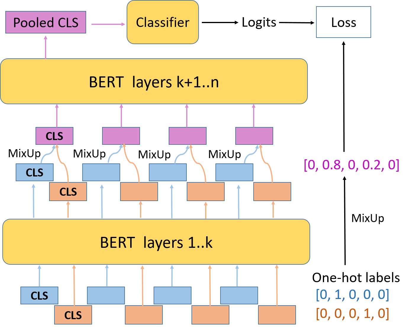
Figure 1: Schematics of Manifold MixUp. We mix the layer $k$ embeddings and the one-hot labels of two training samples using the same proportions $\lambda$ and $(1-\lambda)$ (See eq 1).

4 Results

Our IMDB (Table 2) and AGNews (Table 3) results indicate that Manifold, Input, and CLS MixUp methods improve model robustness and calibration across a range of data regimes; the improvements are more significant when the amount of training data is scarce, which matches our expectation since MixUp can be seen as a form of data augmentation. Manifold MixUp offers the best improvement for model calibration; in fact, the Manifold MixUp model trained on merely 32 samples is equally or more calibrated in comparison to the baseline model trained using the full training set.

Both sentiment analysis on IMDB and news category classification on AGNews are relatively simple tasks that do not necessarily require the model to have syntactic knowledge; instead, they are likely to be solved by only inspecting the sentiment or classification of the individual words. For example, a movie review with more negative words than positive ones is likely to be negative overall. Therefore, we expect Input and Manifold MixUp, which interpolate embeddings at the token level, to work well here; indeed, they outperform baseline and CLS MixUp in these simpler scenarios.

Size	Model	Acc	Loss	ECE
Full	Base	$91.8\pm 0.1$	$61\pm 8$	$7.7\pm 0.1$
	CLS	$92.0\pm 0.1$	$29\pm 1$	$5.8\pm 0.2$
	Input	$92.1\pm 0.1$	$37\pm 2$	$6.8\pm 0.2$
	Mani	$91.8\pm 0.1$	$27\pm 1$	$4.4\pm 0.6$
$32$	Base	$68.2\pm 1.6$	$180\pm 19$	$29.0\pm 1.5$
	CLS	$69.6\pm 1.7$	$86\pm 4$	$21.0\pm 2.8$
	Input	$70.8\pm 1.2$	$61\pm 7$	$8.9\pm 2.3$
	Mani	$72.3\pm 1.0$	$55\pm 2$	$3.4\pm 0.9$

Table 2: MixUp experiments for IMDB using various models (baseline, cls, input, manifold), train sizes. Standard errors over five runs.

Size	Model	Acc	Loss	ECE
Full	Base	$93.7\pm 0.1$	$36\pm 7$	$5.0\pm 0.6$
	CLS	$93.7\pm 0.1$	$28\pm 1$	$4.3\pm 0.3$
	Input	$93.8\pm 0.1$	$25\pm 1$	$4.1\pm 0.3$
	Man	$93.7\pm 0.1$	$23\pm 5$	$3.0\pm 0.2$
$32$	Base	$81.9\pm 0.6$	$72\pm 9$	$9.9\pm 1.9$
	CLS	$83.4\pm 0.6$	$55\pm 2$	$7.2\pm 0.7$
	Input	$82.9\pm 0.3$	$53\pm 2$	$6.2\pm 2.4$
	Mani	$82.3\pm 0.4$	$52\pm 1$	$4.8\pm 1.8$

Table 3: MixUp experiments for AGNews using various train sizes. Standard errors over five runs.

Unlike IMDB and AGNews, the remaining tasks CoLA (acceptability), RTE (NLI), and BoolQ (QA) rely on syntactic knowledge. Therefore, we would expect Input and Manifold MixUp to work relatively poorly for these tasks, since they can disrupt sentence syntax (eg. by interpolating nouns with verbs). This is empirically confirmed when we applied the three MixUp methods to training on the CoLA dataset (Table 4), where the Input and Manifold MixUp models under-perform baseline.

Task	Model	MCC/Acc	Loss	ECE
CoLA	Base	$52.5\pm 0.6$	$56\pm 4$	$11.5\pm 0.3$
	CLS	$52.8\pm 0.6$	$48\pm 1$	$9.7\pm 0.1$
	Input	$50.8\pm 0.8$	$48\pm 8$	$10.1\pm 1.4$
	Mani	$51.0\pm 1.0$	$45\pm 2$	$9.0\pm 0.9$
RTE	Base	$63.8\pm 1.4$	$125\pm 20$	$27.6\pm 1.9$
	CLS	$63.8\pm 1.0$	$80\pm 4$	$20.8\pm 1.3$
BoolQ	Base	$73.4\pm 0.3$	$170\pm 7$	$24.8\pm 0.3$
	CLS	$73.1\pm 0.3$	$89\pm 1$	$21.8\pm 0.3$

Table 4: MixUp experiments for CoLA, RTE, and BoolQ. CoLA is evaluated using Test Matthew Correlation Coefficient (MCC), others using Test Accuracy. Standard errors over five runs.

For the three more advanced tasks, while CLS MixUp exerts negligible effect on the model’s predictive performance, it still significantly reduces test loss and improves calibration without sacrificing performance. The evolution of test losses across training steps for MixUp and baseline models are plotted in Appendix D, demonstrating the ability of MixUp to reduce model overfitting. We note that in contrast to our experiments, Sun et al. (2020) were able to obtain improvements using CLS MixUp for CoLA and RTE using a different training regimen, where MixUp is only applied during the last half of training epochs.

5 Conclusion

In this work, we propose CLS, Input, and Manifold MixUp methods for the transformer architecture and apply them to a range of NLU tasks including sentiment analysis, multi-class classification, acceptability, NLI, and QA. We find that MixUp can improve the predictive performance of simpler tasks. More generally, MixUp can significantly reduce model overfitting and improve model calibration.

Appendix A Calibration Metrics

As in the work of Guo et al. (2017), we calculate the expected calibration error (ECE) of our model as follows: Predictions are grouped into $15$ interval bins of equal size ordered by prediction confidence. Let $B_{m}$ be the set of samples that fall into bin $m$. The accuracy and confidence of $B_{m}$ are defined as:

$$\mathrm{acc}(B_{m})=\frac{1}{|B_{m}|}\sum_{i\in B_{m}}1(\hat{y_{i}}=y_{i})$$

$$\mathrm{conf}(B_{m})=\frac{1}{|B_{m}|}\sum_{i\in B_{m}}\hat{p_{i}}$$

where $\hat{p_{i}}$ is the confidence (winning score) of sample $i$. The Expected Calibration Error (ECE) is then defined as:

$$\mathrm{ECE}=\sum^{M}_{m=1}\frac{|B_{m}|}{n}\Big{|}\mathrm{acc}(B_{m})-\mathrm{conf}(B_{m})\Big{|}$$

Appendix B Padding Options for Input and Manifold MixUp

In the previous MixUp study in language (Guo et al., 2019), all sentences are padded to the same length prior to training using Input MixUp. We believe that while sentences should be padded to the same length, it ought to be done using the minimum amount of padding tokens possible, as the introduction of excessive padding tokens can disrupt performance. Instead of uniformly padding all sentences to length of the longest sentence, we propose to pad pairs of sentences about to be interpolated during training to the length of the longer sentence.

We consider SEP, unused0, PAD tokens from the BERT vocabulary to be potential padding candidates. We empirically evaluate the effect of using each of these paddings for Input MixUp, both when using our proposal (pair) and the one in which all sentences are padded to the length of the longest sequence (max).

We performed padding experiments on SST-2 dataset  (Wang et al., 2018) due to its short training sentence lengths, which leaves more room for padding. We simulate low resource setting by using a random sample of 64 training samples to increase task difficulty, thereby making it easier to detect performance differences.

Our results (Table 5) confirm that pair-wise padding works better than no padding at all as well as the uniform padding of sentences to the maximum length, while the choice of SEP results in the best performance.

Type	Accuracy
No Pad	$78.38\pm 3.2$
unused (pair)	$80.22\pm 1.2$
SEP (pair)	$\boldsymbol{82.00\pm 1.4}$
PAD (pair)	$81.20\pm 1.0$
unused (max)	$68.14\pm 5.3$
SEP (max)	$69.21\pm 5.6$
PAD (max)	$73.61\pm 3.3$

Table 5: The effect of different padding strategies on finetuning BERT on the SST-2 dataset using Input MixUp.

Appendix C Hyperparameters

Hyperparameters for training downstream tasks are shown in Table 6.

	LR	BS	EP	DR	MSL	$\alpha$
IMDB	$1E-5$	$16$	$10$	0.1	$128$	$1.00$
AGNews	$2E-5$	$16$	$10$	0.1	$128$	$1.00$
CoLA	$2E-5$	$16$	$5$	0.1	$128$	$0.75$
RTE	$3E-5$	$16$	$5$	0.1	$128$	$1.00$
BoolQ	$2E-5$	$16$	$10$	0.1	$256$	$1.00$

Table 6: Hyperparameters for training downstream tasks. LR: Learning Rate. BS: Batch Size. EP: Training Epochs. DR: Dropout rate for BERT and classifier. MSL: Maximum Sequence Length. $\alpha$: hyperparameter for beta distribution used in MixUp.

Appendix D Evolution of test loss

Evolution of test losses across training steps for CoLA, RTE, and BoolQ (2) are plotted. MixUp reduces overfitting by allowing the model to converge to a much lower test loss.

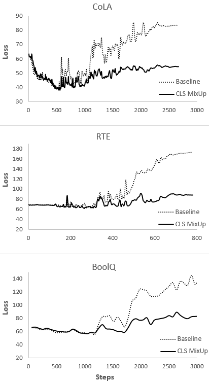
Figure 2: Test losses obtained by the baseline models versus CLS MixUp models across training steps

References

- Desai and Durrett (2020) Shrey Desai and Greg Durrett. 2020. Calibration of pre-trained transformers. arXiv:3003.07892.
- Devlin et al. (2019) Jacob Devlin, Ming-Wei Chang, Kenton Lee, and Kristina Toutanova. 2019. Bert: Pre-training of deep bidirectional transformers for language understanding. In Proceedings of NAACL-HLT.
- Guo et al. (2017) Chuan Guo, Geoff Pleiss, Yu Sun, and Kilian Q. Weinberger. 2017. On calibration of modern neural networks. In Proceedings of the 34th International Conference on Machine Learning.
- Guo et al. (2019) Hongyu Guo, Yongyi Mao, and Richong Zhang. 2019. Augmenting data with mixup for sentence classification: An empirical study. arXiv:1905.08941.
- Maas et al. (2011) Andrew L. Maas, Raymond E. Daly, Peter T. Pham, Dan Huang, Andrew Y. Ng, and Christopher Potts. 2011. Learning word vectors for sentiment analysis. In Proceedings of the 49th Annual Meeting of the Association for Computational Linguistics: Human Language Technologies, pages 142–150, Portland, Oregon, USA. Association for Computational Linguistics.
- Sun et al. (2020) Lichao Sun, Congying Xia, Wenpeng Yin, Tingtin Liang, Philip S. Yu, and Lifang He. 2020. Mixup-transformer: Dynamic data augmentation for nlp tasks. In The 28th International Conference on Computational Linguistics.
- Thulasidasan et al. (2019) Sunil Thulasidasan, Gopinath Chennupati, Jeff Bilmes, Tanmoy Bhattacharya, and Sarah Michalak. 2019. On mixup training: Improved calibration and predictive uncertainty for deep neural networks. In 33rd Conference on Neural Information Processing Systems.
- Verma et al. (2019) Vikas Verma, Alex Lamb, Christopher Beckham, Amir Najafi, Ioannis Mitliagkas, Aaron Courville, David Lopez-Paz, and Yoshua Bengio. 2019. Manifold mixup: Better representations by interpolating hidden states. In Proceedings of the 36th International Conference on Machine Learning.
- Wang et al. (2019) Alex Wang, Yada Pruksachatkun, Nikita Nangia, Amanpreet Singh, Julian Michael, Felix Hill, Omer Levy, and Samuel Bowman. 2019. Superglue: A stickier benchmark for general-purpose language understanding systems. 33rd Conference on Neural Information Processing Systems.
- Wang et al. (2018) Alex Wang, Amanpreet Singh, Julian Michael, Felix Hill, Omer Levy, and Samuel Bowman. 2018. Glue: A multi-task benchmark and analysis platform for natural language understanding. Proceedings of the 2018 EMNLP Workshop BlackboxNLP: Analyzing and Interpreting Neural Networks for NLP.
- Wolf et al. (2019) Thomas Wolf, Lysandre Debut, Victor Sanh, Julien Chaumond, Clement Delangue, Anthony Moi, Pierric Cistac, Tim Rault, R’emi Louf, Morgan Funtowicz, and Jamie Brew. 2019. Huggingface’s transformers: State-of-the-art natural language processing. ArXiv, abs/1910.03771.
- Zhang et al. (2018) Hongyi Zhang, Moustapha Cisse, Yann N. Dauphin, and David Lopez-Paz. 2018. mixup: Beyond empirical risk minimization. In International Conference on Learning Representations.
- Zhang et al. (2015) Xiang Zhang, Junbo Zhao, and Yann LeCun. 2015. Character-level convolutional networks for text classification.