Abstract

In this paper, we learn dynamics models for parametrized families of dynamical systems with varying properties. The dynamics models are formulated as stochastic processes conditioned on a latent context variable which is inferred from observed transitions of the respective system. The probabilistic formulation allows us to compute an action sequence which, for a limited number of environment interactions, optimally explores the given system within the parametrized family. This is achieved by steering the system through transitions being most informative for the context variable.

We demonstrate the effectiveness of our method for exploration on a non-linear toy-problem and two well-known reinforcement learning environments.

1 INTRODUCTION

Learning dynamics models for model-based control and model-based reinforcement learning has recently attracted significant attention by the machine learning community (Chua et al.,, 2018; Hafner et al.,, 2019, 2020). In this paper, we depart from the setting of learning a single forward dynamics model per system. Instead, we learn the dynamics of a distribution of systems which are parameterized by a latent context variable. The latent variable is only observable through the modulations it causes in the dynamics of the systems. Our modeling approach is based on the Neural Processes (NP) (Garnelo et al., 2018b, ) framework: The dynamics model, which is shared across all systems we train on, can be conditioned on context observations from a particular system instance, similar to Gaussian Process dynamics models (Deisenroth and Rasmussen,, 2011). Conditioning on context observations implicitly requires performing inference on the latent variables that govern the dynamics. This process can also be interpreted as a form of meta-learning, as we learn to adapt a shared model for a specific task. Our shared dynamics model then becomes system-specific.

Our main contribution is the proposal of an informed calibration scheme in that framework. We ask the question: Given a system from a family of systems (e.g., the family of pendulums with varying pole masses), what action sequence should one apply to the (unknown) system to identify it as quickly as possible within that family (e.g., to infer the mass of the pendulum’s pole). An optimization procedure seeks for transitions of the system being most informative for the latent variable, while respecting the dynamical constraints of the system.

To this end, we build upon the NP formulation from Garnelo et al., 2018b to construct a context-conditional dynamics model with a probabilistic context encoder which regresses the belief over a latent context variable (Section 3). This allows us to formulate a calibration procedure which optimizes for a sequence of actions that minimizes uncertainty in the latent context variable. We formulate an open-loop and model-predictive calibration algorithm to plan for the optimal sequence of actions to execute. In Figure 1(a) we sketch an overview of our proposed calibration scheme.

On an illustrative toy environment (Section 4.2), we show that the uncertainty in the latent context variable corresponds to the informativeness of the set of context observations about the latent factors.

We also apply our method to a modified "Pendulum" environment from OpenAI Gym (Brockman et al.,, 2016) and a modified "MountainCar" environment (Moore,, 1990) which we both extended by varying properties of the underlying dynamics (Sections 4 and 4.4). Our algorithm exhibits a reasonable and explainable behavior for the given task. The calibration procedure we propose yields a calibration sequence which outperforms a random calibration sequence in terms of prediction accuracy of the conditioned dynamics model.

In summary, our contributions are as follows:

• We apply the framework of Neural Processes (Garnelo et al., 2018b, ) with a probabilistic context encoder to formulate a latent dynamics model. We demonstrate in experiments that the probabilistic model yields meaningful posterior uncertainties in the context variable given observations of dynamical systems.

• Based on this probabilistic formulation, we develop an information-theoretic calibration scheme based on expected information gain (EIG) and model-predictive control (MPC). We further demonstrate that our calibration scheme outperforms a baseline which generates actions randomly.

Code and further resources to reproduce the experiments are available at
https://explorethecontext.is.tue.mpg.de.

2 RELATED WORK

Neural Processes

The idea of context-conditional modeling of distributions over functions using a permutation invariant context embedding was first introduced by Garnelo et al., 2018a as Conditional Neural Processes (CNPs). The authors apply CNPs on image completion and classification tasks. While Garnelo et al., 2018a mainly use a deterministic belief for the context encoding, also a latent variable model is introduced, but a deterministic influence of the latent context encoding on function predictions remains. Garnelo et al., 2018b present a more formal treatment of the latent variable model formulation coined Neural Processes (NPs). Sequential Neural Processes (Singh et al.,, 2019) extend the original Neural Processes formulation by a temporal dynamics model on the latent context embedding. Another application of the Neural Process framework has recently been proposed for the domain of learning dynamics models for physics-based systems (Zhu et al.,, 2020). We ground our work on these results to learn a model which allows to globally reason about the uncertainty in the dynamics from the uncertainty in the context encoding, which is crucial for our proposed calibration approaches.

Dynamics Model Learning

In the seminal PILCO approach (Deisenroth and Rasmussen,, 2011), Gaussian Process (GP) dynamics models are learned for control tasks such as cart-poles. Fraccaro et al., (2017) propose an approach for modelling systems with partial observability through linear time-dependent models, with state inference performed by Kalman filtering in the latent space of a variational autoencoder. To enable planning in the learned dynamics models, Watter et al., (2015) learn locally linear models. Probabilistic dynamics models in combination with planning based on the cross-entropy method (Rubinstein,, 1999) have shown to outperform model-free reinforcement learning approaches in terms of sample efficiency (Chua et al.,, 2018) and can be trained directly on image representations (Hafner et al.,, 2019). These methods do not consider variations in the underlying system which can be explained through context variables. We develop a probabilistic context-dependent dynamics model and an information-theoretic planning scheme for calibration based on model-predictive control.

Meta-Learning

Neural and Gaussian Processes can be seen as types of meta learning algorithms which facilitate few-shot learning of the data distribution (Garnelo et al., 2018b, ; Garnelo et al., 2018a, ). Meta learning of dynamics models has been explored in the domain of model-based reinforcement learning (Nagabandi et al.,, 2019; Sæmundsson et al.,, 2018). Nagabandi et al., (2019) propose to combine gradient-based (Finn et al.,, 2017) and recurrence-based (Duan et al.,, 2016) meta learning for online adaptation of the dynamics model. Different to our approach, this meta learning scheme does not explicitly model the dynamics model dependent on a context variable. Calibration on the target system requires fine-tuning the deep neural network. We propose a deep probabilistic model and a learning scheme which allows for inferring such a context variable through calibration. Similar to our approach Sæmundsson et al., (2018) include a latent context variable into a probabilistic hierarchical dynamics model which they choose to model using Gaussian Processes. The method uses probabilistic inference to determine a Gaussian context variable from data. We use a deep encoder to regress probabilistic beliefs on the context variable and propose an information-theoretic approach for dynamics model calibration.

Active Learning and Exploration

The method we propose for system calibration differs in substantial points from what is termed exploration in reinforcement learning. While in exploration the goal of the agent is to visit previously unseen regions of the state space for potentially finding behaviors yielding higher returns, we assume to stay in the domain of systems we observed during training. However, some concepts from exploration approaches in reinforcement learning translate to our method, especially those based on uncertainty- and information-theoretic active learning principles (Epshteyn et al.,, 2008; Golovin et al.,, 2010; Shyam et al.,, 2019; Sekar et al.,, 2020; Tschantz et al.,, 2020). Buisson-Fenet et al., (2020) develop an active learning approach for GP dynamics models exploiting the GP predictive uncertainty. Popular examples of active learning strategies are expected error reduction (EER) (Roy and McCallum,, 2001) or expected information gain (EIG) (MacKay,, 1992). Our information-theoretic calibration approach is formulated based on a variant of EIG.

Optimal Experimental Design

Broadly speaking, the idea of Optimal Experimental Design is to select experiments which reveal maximal information about quantities of interest (Franceschini and Macchietto,, 2008). An information theoretic approach based on EIG as utility function dates even back to the 1950s (Lindley,, 1956). Foster et al., (2019) propose variational approximations for EIG estimation to infer an informative sequence of experiments. Differently, we learn a context-dependent dynamics model which facilitates EIG estimation from the latent context posterior under dynamics constraints. However, their approach relates to our method as they proposed to use function approximators for amortized inference, which is similar to our context encoder, giving an amortized posterior for the latent context variable.

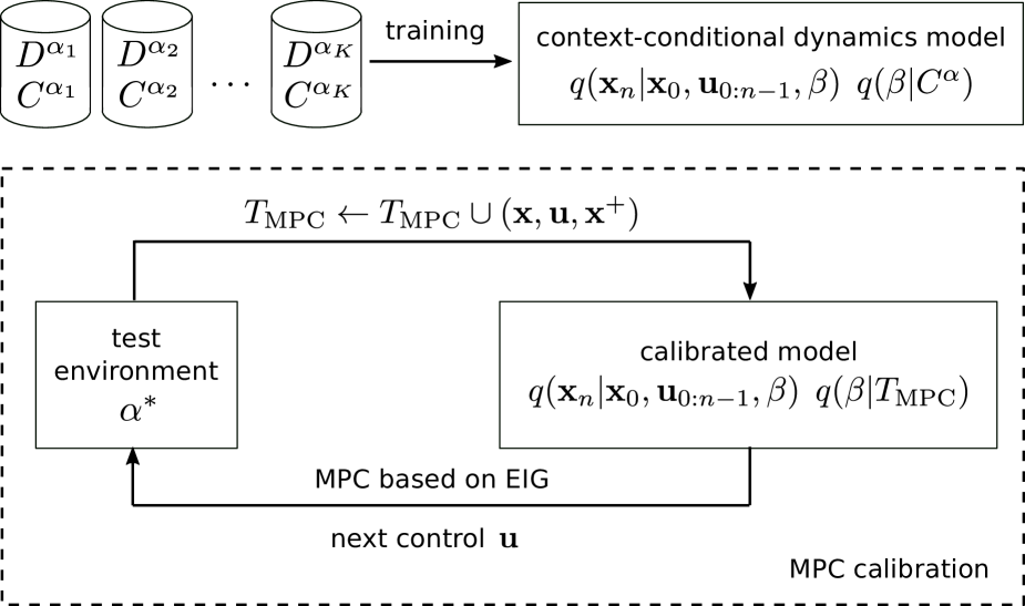
(a) Overview of our proposed model training and model-predictive calibration approach. First, we learn a context-conditional dynamics model on rollouts from a set of $K$ parameterized environments which yield target data ($D^{\alpha}_{1}...D^{\alpha}_{K}$) and context data ($C^{\alpha}_{1}...C^{\alpha}_{K}$). To optimally calibrate a previously unseen test environment $\alpha^{*}$, we employ the context-conditional model for active data collection in a model-predictive control scheme. We then obtain the calibrated model by conditioning on the observations from the calibration rollout $T_{\text{MPC}}$.

(b) Graphical model depicting the proposed context-conditional forward dynamics. The action-conditioned Markovian dynamics are modeled deterministically in a latent space. Observations ${\bm{x}}_{n}$ of the system are random variables conditioned on their respective latent state ${\bm{z}}_{n}$. The dynamics are conditioned on actions $\mathbf{u}_{n}$ and a latent context belief $\bm{\beta}$ which encodes an observed context set $C^{\alpha}$. For prediction, the initial latent state is inferred from the first observation ${\bm{x}}_{0}$ (dashed line).

Figure 1: (a) overview of our proposed calibration approach and (b) context-conditional dynamics model.

3 METHOD

We assume that the observed data of a dynamical system is generated by the following parametrized Markovian discrete-time state-space model

$${\bm{x}}_{n+1}=f({\bm{x}}_{n},{\bm{u}}_{n},\bm{\alpha})+\bm{\epsilon}$$ (1)

with $n\in\mathbb{N}_{0}$, ${\bm{x}}_{n}\in\mathcal{X}\subseteq\mathbb{R}^{\mathrm{dim}(\mathcal{X})}$, ${\bm{x}}_{0}\in\mathcal{X}_{0}\subseteq\mathcal{X}$, ${\bm{u}}_{n}\in\mathcal{U}\subseteq\mathbb{R}^{\mathrm{dim}(\mathcal{U})}$, $\bm{\alpha}\in\mathcal{A}\subseteq\mathbb{R}^{\mathrm{dim}(\mathcal{A})}$, $\bm{\epsilon}\sim\mathcal{N}(0,{\bm{Q}})$. In the following, the term rollout of length $N$ refers to a sequence of states and actions $[{\bm{x}}_{0},{\bm{u}}_{0},{\bm{x}}_{1},{\bm{u}}_{1},...,{\bm{u}}_{N-1},{\bm{x}}_{N}]$, with equation 1 holding for each transition $({\bm{x}}_{n},{\bm{u}}_{n},{\bm{x}}_{n+1})$.

The target data ${D}^{\alpha}$ consists of rollouts of the system for fixed parameters $\bm{\alpha}$ and randomly sampled initial states ${\bm{x}}_{0}$ and action sequences ${\bm{u}}_{0:N-1}:=[{\bm{u}}_{0},...,{\bm{u}}_{N-1}]$. Context data $C^{\alpha}=\left\{({\bm{x}},{\bm{u}},{\bm{x}}^{+})\right\},{\bm{x}}^{+}=f({\bm{x}},{\bm{u}},\bm{\alpha})+\bm{\epsilon}$ is a set of transitions generated by the system with parameters $\bm{\alpha}$. We aim at determining a probabilistic context-conditional dynamics model $p({\bm{x}}_{n}|{\bm{x}}_{0:n-1},{\bm{u}}_{0:n-1},C^{\alpha})$ which maximizes the expected data log-likelihood

$$\max\>\mathbb{E}_{\alpha\sim{A}}\left[\log p(D^{\alpha}|C^{\alpha})\right]$$ (2)

where ${A}$ denotes the empirical distribution of parameter values $\bm{\alpha}$ and $p(D^{\alpha}|C^{\alpha})=\prod_{n=1}^{N}p({\bm{x}}_{n}|{\bm{x}}_{0:n-1},{\bm{u}}_{0:n-1},C^{\alpha})$. For a graphical depiction of our modeling approach, see Figure 1(b).

Latent context variable

Since we cannot directly observe $\bm{\alpha}$ and also do not know its representation, we introduce a latent variable $\bm{\beta}\in\mathbb{R}^{B}$ whose representation we learn and which encodes context information corresponding to $\bm{\alpha}$ contained in the context set,

$$\log p(D^{\alpha}|C^{\alpha})=\log\int p(D^{\alpha}|\bm{\beta})p(\bm{\beta}|C^{\alpha})\,\mathrm{d}\bm{\beta}.$$ (3)

We model $p(D^{\alpha}|\bm{\beta})$ by $q(D^{\alpha}|\bm{\beta})=\prod_{n=1}^{N}q({\bm{x}}_{n}|{\bm{x}}_{0},{\bm{u}}_{0:n-1},\bm{\beta})$ with transition model $q({\bm{x}}_{n}|{\bm{x}}_{0},{\bm{u}}_{0:n-1},\bm{\beta})$ and approximate $p(\bm{\beta}|C^{\alpha})$ by $q(\bm{\beta}|C^{\alpha})$, the context encoder.

Transition model

To model transition sequences of length $H$ starting at index $n$, we assume non-linear dynamics parametrized by $\bm{\beta}$ and disturbed by additive zero-mean Gaussian noise $\bm{\epsilon}$

$$\bm{\hat{x}}_{n+H}=h({\bm{x}}_{n},{\bm{u}}_{n},...,{\bm{u}}_{n+H-1},\bm{\beta})+\bm{\epsilon}.$$ (4)

We implement the dynamics by a recurrent GRU cell (Cho et al.,, 2014) which operates in an embedding space. The encoders $g_{\mathrm{state}}$, $g_{\mathrm{action}}$ and $g_{\bm{\beta}}$ lift, respectively, the state observation ${\bm{x}}_{n}$, action ${\bm{u}}_{n}$ and latent context variable $\bm{\beta}$ to the embedding space in which the GRU operations are performed

$$\begin{split}{\bm{z}}_{n}&=g_{\mathrm{state}}({\bm{x}}_{n}),\\ {\bm{z}}_{n+1}&=h_{\mathrm{RNN}}({\bm{z}}_{n},[g_{\mathrm{action}}(\bm{u}_{n}),{g_{\bm{\beta}}}(\bm{\beta})])\end{split}$$ (5)

where $[\cdot,\cdot]$ denotes concatenation. The decoders $d_{\mathrm{state},\mu}$ and $d_{\mathrm{state},\sigma^{2}}$ map the propagated hidden state back to a distribution on the state space

$$\bm{\hat{x}}_{n+H}\sim\mathcal{N}(d_{\mathrm{state},\mu}({\bm{z}}_{n+H}),\mathrm{diag}(d_{\mathrm{state},\sigma^{2}}({\bm{z}}_{n+H})).$$ (6)

Context encoder

The context encoder $q(\bm{\beta}|C^{\alpha})$ encodes a set of transitions $C^{\alpha}$ into a Gaussian belief over the latent context variable

$$q(\bm{\beta}|C^{\alpha})=\mathcal{N}\left(\bm{\beta}\>|\>{\bm{\mu}_{\bm{\beta}}}(C^{\alpha}),{\mathrm{diag}(\bm{\sigma^{2}}_{\bm{\beta}}}(C^{\alpha})\right).$$ (7)

As a first step of the encoding procedure, every transition is lifted separately into an embedding space $\mathcal{Z}=\mathbb{R}^{Z}_{\geq 0}$ using the transition encoder $g_{\mathrm{trans}}$, which is non-negative due to its terminal ReLU activation function. Then, the embedded transitions are aggregated by max pooling, making the aggregated embedding invariant to the ordering of transitions in the context set $C^{\alpha}$, which is a common set embedding technique (Zaheer et al.,, 2017; Garnelo et al., 2018a, )

$$g_{\mathrm{trans}}:\mathcal{X}\times\mathcal{U}\times\mathcal{X}\rightarrow\mathcal{Z},\>\bm{z}=g_{\mathrm{trans}}(\bm{x},\bm{u},\bm{x}^{+})$$ (8)

$$[{\bm{z}_{\bm{\beta}}}]_{i}=\max_{(\bm{x},\bm{u},\bm{x}^{+})\in{C^{\alpha}}}[g_{\mathrm{trans}}(\bm{x},\bm{u},\bm{x}^{+})]_{i}.$$ (9)

where $[\cdot]_{i}$ denotes the $i$-th element of a vector. For an empty context set, we fix ${\bm{z}_{\bm{\beta}}}=0$. The mean and diagonal elements of the covariance matrix of the Gaussian belief over $\bm{\beta}$ are computed from the aggregated embedding using multilayer perceptrons

$${\bm{\hat{\mu}}_{\bm{\beta}}}:\mathcal{Z}\rightarrow\mathbb{R}^{B},\quad{\bm{\hat{\sigma}^{2}}_{\bm{\beta}}}:\mathcal{Z}\rightarrow\mathbb{R}^{B}_{>0}.$$ (10)

While ${\bm{\hat{\mu}}_{\bm{\beta}}}$ follows a standard architecture, we structure ${\bm{\hat{\sigma}^{2}}_{\bm{\beta}}}$ to resemble the behavior of Bayesian inference of a latent variable given noisy measurements (Murphy,, 2012). In this setting, adding a datapoint to the set of measurements cannot increase uncertainty over the latent variable. Due to the non-negativity of $g_{\mathrm{trans}}$ and the monotonicity of the max pooling operation, this can be achieved by requiring ${\bm{\hat{\sigma}^{2}}_{\bm{\beta}}}(\cdot)$ to be monotonically decreasing in the sense

$$\begin{split}[{\bm{\hat{\sigma}^{2}}_{\bm{\beta}}}(\bm{z})]_{i}\geq[{\bm{\hat{\sigma}^{2}}_{\bm{\beta}}}(\bm{z}+\bm{\Delta_{z}})]_{i}\\ \forall\bm{z}\in\mathbb{R}^{Z}_{\geq 0},\bm{\Delta_{z}}\in\mathbb{R}^{Z}_{\geq 0},i\in\{1,...,B\}.\end{split}$$ (11)

To model this strictly positive, monotonically decreasing function, we squash the negated output of a multilayer perceptron having non-negative weights and activations, ${g_{\mathrm{non-neg}}}({\bm{z}_{\bm{\beta}}})$ through a Softplus activation function $\zeta(x)=\ln(1+\exp(x))$

$${\bm{\hat{\sigma}^{2}}_{\bm{\beta}}}({\bm{z}_{\bm{\beta}}})=\zeta\left(-g_{\mathrm{non-neg}}({\bm{z}_{\bm{\beta}}})\right).$$ (12)

We fix the scale of the latent belief by forcing the latent belief for an empty context set to the unit Gaussian $\mathcal{N}(0,\bm{I})$ with a KL divergence penalty term $\mathcal{L}_{\mathrm{KL}}=\mathrm{KL}(q(\bm{\beta}|C^{\alpha}=\{\})\|\mathcal{N}(0,\bm{I}))$.

Evidence maximization

For general non-linear dynamics models, the integral in equation 3 cannot be solved analytically. Similar to Garnelo et al., 2018b , we formulate a lower bound on the log evidence

$$\begin{split}&\log p(D^{\alpha}|C^{\alpha})\geq\mathcal{J}\\ &\quad=\mathbb{E}_{\bm{\beta}\sim q(\bm{\beta}|D^{\alpha}\cup C^{\alpha})}\left[\mathcal{J}_{\mathrm{logll}}(D^{\alpha},\bm{\beta})\right]\\ &\quad\quad-\lambda_{\mathrm{KL}}\mathrm{KL}(q(\bm{\beta}|D^{\alpha}\cup C^{\alpha})\>||\>q(\bm{\beta}|C^{\alpha}))\end{split}$$ (13)

where $\mathcal{J}_{\mathrm{logll}}$ denotes the log-likelihood of a target chunk $D^{\alpha}=[{\bm{x}}_{n},{\bm{u}}_{n},{\bm{x}}_{n+1},...,{\bm{u}}_{n+H-1},{\bm{x}}_{n+H}]$ and $\lambda_{\mathrm{KL}}$ is a weighting factor for the KL divergence. To reduce gradient variance, especially in the beginning of training, we evaluate $\mathcal{J}_{\mathrm{logll}}=\mathcal{J}_{\mathrm{ms}}+\mathcal{J}_{\mathrm{ss}}+\mathcal{J}_{\mathrm{rec}}$ as a combination of multi-step and single-step prediction log-likelihood and the immediate reconstruction likelihood in each time step.

The multi-step log-likelihood is given by $\mathcal{J}_{\mathrm{ms}}=\sum_{h=2}^{H}\log q(\bm{{x}}_{n+h}|{\bm{x}}_{n},{\bm{u}}_{n:n+h-1},\bm{\beta}),$ while the term for single-step predictions is $\mathcal{J}_{\mathrm{ss}}=\sum_{h=0}^{H-1}\log q(\bm{{x}}_{n+h+1}|{\bm{x}}_{n+h},{\bm{u}}_{n+h},\bm{\beta}).$ The reconstruction term is $\mathcal{J}_{\mathrm{rec}}=\sum_{h=0}^{H}\log q({\bm{{\hat{x}}}_{n+h}=\bm{{x}}_{n+h}}|{\bm{x}}_{n+h}).$

The final loss $\mathcal{L}$ we minimize states

$$\mathcal{L}=-\mathcal{J}+\mathcal{L}_{\mathrm{KL}}.$$ (14)

Further architectural details are given in the supplementary material.

3.1 Computing optimal action sequences for calibration

We will now discuss algorithms to utilize the learned models from above to define optimal calibration schemes. We refer to "calibration" as the process of inferring unknown latent variables governing the dynamics of a system, while assuming that the model is a member of the family of dynamics models seen during training.

We formulate finding optimal actions to apply to a system for calibration as a Bayesian optimal experimental design problem with an information-theoretic utility function (Lindley,, 1956; Chaloner and Verdinelli,, 1995). We choose an action sequence ${\bm{u}}_{0},...,{\bm{u}}_{N-1}$ to maximize the expected information gain

$$\begin{split}&\mathrm{EIG}({\bm{u}}_{0:N-1}|{\bm{x}}_{0},{T}_{0})=\\ &\mathbb{E}_{{T}\sim q({T}|{\bm{x}}_{0},{\bm{u}}_{0:N-1},{T}_{0})}\left[H[q(\bm{\beta}|{T}_{0})]-H[q(\bm{\beta}|{T}_{0}\cup{T})]\right]\end{split}$$ (15)

where ${\bm{x}}_{0}$ is the current state of the system, ${T}_{0}$ are already observed transitions on the system to calibrate and $H[\cdot]$ represents the entropy. The belief over the latent context variable $q(\bm{\beta}|{T})$ after observing a set of calibration transitions ${T}$ is given by the context encoder. The distribution of imagined rollouts of the system $q({T}|{\bm{x}}_{0},{\bm{u}}_{0},...,{\bm{u}}_{N-1},{T}_{0})$ is generated from the multi-step transition model while marginalizing out the prior belief over the latent context variable

$$\begin{split}&q({T}|{\bm{x}}_{0},{\bm{u}}_{0:N-1},{T}_{0})=\\ &\quad\int q({T}|{\bm{x}}_{0},{\bm{u}}_{0:N-1},\bm{\beta})q(\bm{\beta}|{T}_{0})\mathrm{d}\bm{\beta}.\end{split}$$ (16)

We get a Monte Carlo approximation to the expectation in equation 15 by approximate sampling from the above distribution. To obtain a sample, we first sample from the latent context distribution $\bm{\beta}_{0}\sim q(\bm{\beta}|{T}_{0})$. Next, we form the set of calibration transitions ${T}=\{({\bm{x}}_{n},{\bm{u}}_{n},{\bm{x}}_{n+1})\}_{n=\{0,...N-1\}}$, where ${\bm{x}}_{n}$ for all $1\leq n\leq N$ are predictions from the learned transition model ${\bm{x}}_{n}=\mathbb{E}[q({\bm{x}}_{n}|{\bm{x}}_{0},{\bm{u}}_{0},...,{\bm{u}}_{n-1},\bm{\beta}_{0})]$.

The action sequence which the $\mathrm{EIG}$ maximization yields is most informative for the latent context variable (minimizes the posterior entropy) given the a-priori belief, i.e., taking the a-priori uncertainty about the context variable into account.

Open-Loop calibration

In the open-loop calibration case, we initialize the set of already observed transitions as the empty set ${T}_{0}=\{\}$. We then optimize for a sequence of actions ${\bm{u}}_{0}^{*},...,{\bm{u}}_{N-1}^{*}$ to fulfill

$$\begin{split}&{\bm{u}}_{0}^{*},...,{\bm{u}}_{N-1}^{*}=\\ &\quad\operatorname*{arg\,max}_{{\bm{u}}_{0},...,{\bm{u}}_{N-1}\in\mathcal{U}}\mathrm{EIG}({\bm{u}}_{0},...,{\bm{u}}_{N-1}|{\bm{x}}_{0},{T}_{0}=\{\})\end{split}$$ (17)

using the cross-entropy method (Rubinstein,, 1999). We call $N$ calibration horizon.

MPC calibration

The Open-Loop calibration scheme computes a static action sequence at the beginning of the calibration procedure. The planned action sequence is not updated during calibration. However, knowledge about the system obtained through already executed system interactions may be valuable to re-plan the remaining calibration actions. Therefore, we propose a calibration method which resembles a model-predictive control scheme known from feedback control theory, which we term MPC calibration. For MPC calibration, we compute an Open-Loop calibration sequence at every timestep, with ${T}_{n}$ containing already observed transitions (${T}_{0}=\{\}$). From this calibration sequence, the first action is applied to the system and the resulting transition is appended to ${T}_{n}$, giving ${T}_{n+1}$. This is repeated for a fixed number of timesteps $N$. Let ${\bm{x}}_{n}$ be the current state of the system and ${T}_{n}$ contain already observed transitions. At each timestep, we optimize

$$\begin{split}&{\bm{u}}_{n}^{*},...,{\bm{u}}_{n+H-1}^{*}=\\ &\quad\operatorname*{arg\,max}_{{\bm{u}}_{n},...,{\bm{u}}_{n+H-1}\in\mathcal{U}}\mathrm{EIG}({\bm{u}}_{n},...,{\bm{u}}_{n+H-1}|{\bm{x}}_{n},{T}_{n}),\end{split}$$ (18)

and apply ${\bm{u}}_{n}^{*}$ as next action to the system. The planning horizon $H$ is upper bounded by the maximal planning horizon $H_{\mathrm{max}}$ and the remaining steps to reach the calibration horizon as $H=\min(H_{\mathrm{max}},N-n)$. Due to the repeated optimization, the MPC calibration scheme is more computationally intensive than the Open-Loop scheme.

4 EXPERIMENTS

We evaluate our approach for learning and calibrating context-dependent dynamics models on an illustrative toy problem, a modified Pendulum environment from OpenAI Gym and a MountainCar environment with randomly sampled terrain profiles. We present further ablation studies in the supplementary material.

4.1 General procedure

Data collection

For each experiment, we collect random data from the respective environments. For this, we first sample environment instances for each experiment, varying in their hidden parameters $\bm{\alpha}$. The respective samples of $\bm{\alpha}$ constitute the empirical distribution $A$. Then, we simulate two rollouts of length 100 on each sampled environment instance, by applying independently sampled actions starting from a random initial state. More specific details are given in the "Data collection" paragraph of each experiment.

Model training

From the pre-generated data, we sample target chunks $D^{\alpha}$ and context sets $C^{\alpha}$ for empirical loss minimization

$$\min\>\mathbb{E}_{\alpha\sim{A},D^{\alpha},C^{\alpha}}\left[\mathcal{L(D^{\alpha},C^{\alpha})}\right],$$ (19)

where $A$ denotes the empirical distribution of parameter values $\bm{\alpha}$. We refer to the supplementary material for details on the sampling procedure. We train all models using the Adam optimizer (Kingma and Ba,, 2015). For evaluation, we select the model which reaches minimal validation loss within 50k steps for the toy problem and 100k steps for Pendulum and MountainCar. We perform all evaluations on 3 independently trained models per environment and model configuration. We set the KL divergence scaling factor in equation 13 to $\lambda_{\mathrm{KL}}=5$. For more details on the training procedure, we refer to the supplementary material.

4.2 Toy system

First, we introduce an illustrative toy-problem showcasing the fundamental principles of our method. It is a discrete-time dynamical system in state-space notation

$${\bm{x}}_{n+1} =\begin{pmatrix}0.8&0.2\\ -0.2&0.8\end{pmatrix}{\bm{x}}_{n}+\begin{pmatrix}\alpha\\ 0\end{pmatrix}\delta(u_{n})+\bm{\epsilon}$$ (20)

with $\bm{\epsilon}\sim\mathcal{N}(0,\bm{I}\cdot(0.01)^{2}),\bm{x}_{0}\sim\mathcal{N}(0,\bm{I}),\alpha\in[-1,1],u_{n}\in[-2,2]$. The state transition matrix leads to a damped oscillation when the system is not excited. A non-linear function $\delta$ squashes the input $u_{n}$ before it is applied to the system. Inference about the parameter $\alpha$ from empirical system trajectories is only possible when at least one transition $({\bm{x}}_{n},u_{n},{\bm{x}}_{n+1})$ is observed with $\delta(u_{n})\neq 0$. As squashing functions we define $\delta^{<1}(u_{n})=\max(1-|u_{n}|,0)$ and $\delta^{>1}(u_{n})=\max(|u_{n}|-1,0)$, with the superscript denoting which $u_{n}$ are mapped to non-zero values, thus, being informative for the value of $\alpha$. We train separate models for each squashing function $\delta^{<1}(u_{n})$, $\delta^{>1}(u_{n})$. As we assume homoscedastic noise in this experiment, we learn a constant $d_{\mathrm{state},\sigma^{2}}$ independent of $\bm{z}$.

Data collection

To collect training and validation data, we sample 6k values of $\alpha\sim\mathrm{Uniform}[-1,1]$ and generate a rollout pair for each $\alpha$, with the initial state sampled from $\bm{x}_{0}\sim\mathcal{N}(0,\bm{I})$ and the control inputs from $u_{n}\in\mathrm{Uniform}[-2,2]$.

Evaluation

As a first evaluation, we visualize the entropy of the latent context variable for informative and non-informative context sets. We generate random transitions $({\bm{x}}_{0},u,{\bm{x}}_{1})$ with $\bm{\beta}\sim q(\bm{\beta}|C^{\alpha}=\{\})$, ${\bm{x}}_{0}=0$, $u_{n}\sim\mathrm{Uniform}[-2,2]$ using the learned transition models for both squashing functions $\delta^{<1}(u_{n})$ and $\delta^{>1}(u_{n})$. We use the learned model instead of the known ground-truth model for generating transitions to simulate the first step of a calibration procedure, in which the true model is unknown. From each transition, we construct a single-element context set and compute the latent context belief using the learned context encoder. In Figure 2, we plot the entropy of the latent context belief for each action $u_{n}$, averaged over samples from $\bm{\beta}$. For the posed systems with $\delta^{<1}(u_{n})$ ($\delta^{>1}(u_{n})$), a single-element context is informative for $\alpha$ if and only if it contains a transition with an action $|u_{n}|<1$ ($|u_{n}|>1$). We observe that the entropy is minimized correspondingly for our learned model which demonstrates that the context encoder predicts uncertainty well.

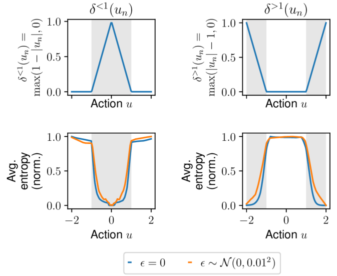
Figure 2: Characteristic behavior of the latent context belief encoder on the toy problem. First row: Depiction of the action squashing functions $\delta^{<1}(u_{n})$, $\delta^{>1}(u_{n})$ (effective action magnitude). Action regions which are informative for inferring the hidden parameter $\alpha$ are shaded in gray ($\delta(u_{n})\neq 0$). Second row: Average entropy (normalized to $[0,1]$) of the latent context belief $H[q(\beta|C=\{\bm{x},{u},\bm{x}^{+}\})]$ for actions ${u}$ in systems with Gaussian observation noise $\bm{\epsilon}\sim\mathcal{N}(0,\bm{I}\cdot(0.01)^{2})$ (orange) and $\bm{\epsilon}=0$ (blue). Non-informative actions yield a high entropy of the latent context belief, for informative actions, the entropy negatively correlates to the effective action magnitude. Without observation noise, the entropy attains its minimum faster for increasing effective action magnitude as $\alpha$ can be inferred from low-magnitude actions with low variance.

In a second experiment, we evaluate the model accuracy in terms of prediction error after calibration on a set of random rollouts for 3 independently trained models. We sample 50 system instances with $\alpha\sim\mathrm{Uniform}[-1,1]$, and for each instance we generate 20 random rollouts. For calibration, we limit the maximum number of transitions to $\{1,2,3\}$ and perform open-loop calibration (see section 3.1) on each system instance. As baseline, we use randomly sampled transitions for calibration. Each calibration rollout is initialized at ${\bm{x}}_{0}=0$, for the random calibration rollouts we uniformly sample actions from $\mathrm{Uniform}[-2,2]$. In Figure 3 we depict the mean squared prediction error of the learned models for open-loop optimal and random calibration sequences of different lengths. The prediction error is significantly lower for optimally calibrated models compared to randomly calibrated models. As a single informative transition is sufficient to calibrate the system, MPC calibration has no advantage over Open-Loop calibration for this system.

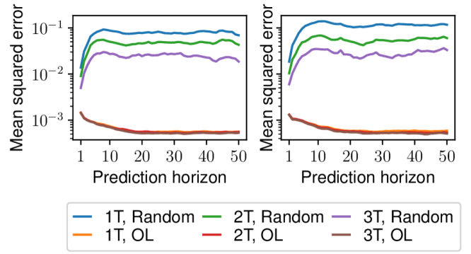
Figure 3: Evaluation of model prediction error for the toy problem. Depicted is the prediction error (lower is better) of models with random and optimal (open-loop) calibration with $\{1,2,3\}$ calibration transitions, for both action squashing schemes $\delta^{<1}(u_{n})$ (left) and $\delta^{>1}(u_{n})$ (right).

4.3 OpenAI Gym Pendulum

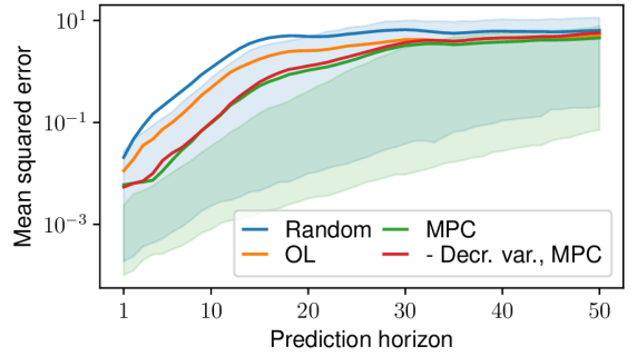
(a) Pendulum

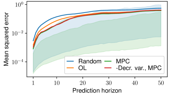
(b) MountainCar

Figure 4: Prediction error (lower is better) of the learned (a) Pendulum and (b) MountainCar models, either conditioned on calibration data obtained with a random rollout (blue), Open-Loop calibration (orange), MPC calibration (green). For the red curve, we train models without the strictly-decreasing variance constraint in the context encoder and perform MPC calibration. We plot mean (line) and $20\%$ / $80\%$ quantiles (shaded area, for random and MPC calibration only for visual clarity) over 3000 rollouts. Our proposed calibration schemes reduce prediction error compared to random calibration. MPC calibration compares favourably to Open-Loop calibration. Enforcing the decreasing variance constraint in the context encoder slightly reduces model error after calibration for Pendulum. For MountainCar, both model variants perform similarly. Calibration rollouts contain 30 transitions for the Pendulum and 50 transitions for the MountainCar environment.

In addition to the toy problem presented above, we evaluate our calibration method on a modified Pendulum environment from OpenAI Gym (Brockman et al.,, 2016). The Pendulum environment is a simulation of an inverted pendulum subject to gravitational force and actuable by a motor in the central rotary joint (see Figure 5(a)). Due to torque limits, the pendulum cannot reach an upright pose without following a swing-up trajectory.

After the motor torque $u$ is clipped to a maximum magnitude of $2$, we multiply it with an angle-dependent factor $u\leftarrow u\cdot s_{i}\cdot\alpha_{i}$. The sign $s_{i}$ and factor $\alpha_{i}$ are sampled independently for every quadrant of the pendulum system ($i\in\{1,2,3,4\}$) from $\alpha_{i}\sim\mathrm{Uniform}[0.5,2]$, $s_{i}\sim\mathrm{Uniform}\{-1,1\}$ (see Figure 5(a)).

Data collection To collect training and validation data, we first sample 110k environments with $s_{i}$ and $\alpha_{i}$ sampled as above. For each environment, we generate 2 independent rollouts with $u_{n}\sim\mathrm{Uniform}[-2,2]$ and ${\bm{x}}_{0}\sim\mathrm{Uniform}[-\pi,\pi]\times\mathrm{Uniform}[-8,8]$, with the first dimension being the pendulum angle and the second dimension its angular velocity.

Evaluation The initial state of the pendulum for calibration is sampled from $\mathrm{Uniform}[\pi-0.05,\pi+0.05]\times\mathrm{Uniform}[-0.05,0.05]$, i.e. with the pole pointing nearly downwards with small angular velocity. In contrast to the toy problem, we use the MPC calibration scheme with a CEM planning horizon of $H_{\mathrm{max}}=20$ and a calibration rollout length of $30$. To approximate the expected information gain from equation 15, we use 20 Monte Carlo samples. We generate 50 environments for calibration with independently sampled $s_{i}$, $\alpha_{i}$. For each environment, we generate 20 random rollouts with ${\bm{x}}_{0}$, $u_{n}$ sampled as in the "Data collection" paragraph. On each environment, we apply our proposed calibration schemes and compare the predictive performance of the learned dynamics model for Open-Loop, MPC and random calibration. For random calibration, we sample random actions $u_{n}\sim\mathrm{Uniform}[-2,2]$.

Figure 5(b) depicts the angle of the pendulum over time for random and MPC calibration rollouts. Due to gravitational forces and inertia of the pendulum, the rollouts only cover the lower two quadrants. Thus, with these random calibration rollouts, the dynamics in the upper two quadrants cannot be inferred. In contrast, the MPC rollouts exhibit a swing-up behavior to reason about the dynamics in all four quadrants. Note that this behavior solely comes from the objective to miminize entropy over the latent context variable and not through explicit modelling, e.g. via rewards.

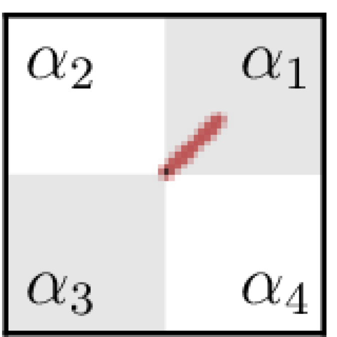
(a) Pendulum dynamics vary per quadrant. The pendulum pole is depicted in red.

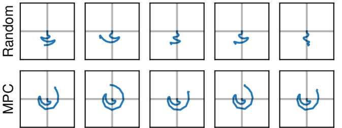
(b) Pendulum angle extruded over time (starting at center) for random and MPC calibration rollouts. In contrast to random calibration rollouts, MPC calibration rollouts cover all quadrants to infer their dynamics.

Figure 5: Properties of the Pendulum environment

In Figure 4(a) we show the prediction error of the learned dynamics model when calibrated in the Open-Loop, MPC and random scheme. For each predicted state we compute the mean squared error to the ground-truth state (with the angle represented as $[\sin(\theta),\cos(\theta)]$) and plot its statistics (mean and quantiles) aggregated over 50 randomly sampled systems, 20 rollouts per system and 3 independently trained models, giving 3000 rollouts. Similarly to the results from section 4.2, the prediction error for models calibrated with the proposed calibration schemes is lower than when calibrated with random system interventions.

As for the pendulum task in principle a single transition is sufficient to infer the dynamics in the quadrant covered by the transition, one can expect that (1) the entropy of the latent context belief decreases for an increasing number of quadrants covered by a context set; (2) adding transitions from an already covered quadrant to the context set does not lead to a strong reduction of entropy; (3) the entropy is minimized when all four quadrants are covered. Our learned context encoder features all of those properties, as we evaluate in Figure 6. The figure depicts how the information (entropy) of the latent context belief behaves for different context sets covering different numbers of quadrants. See Figure 6 for more details.

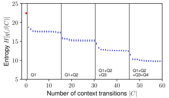
Figure 6: Entropy of the latent context belief mainly depends on the number of covered quadrants by the context set and is barely affected by the number of context transitions larger one in each quadrant. We randomly generate 15 transitions with $u\sim\mathrm{Uniform}[-1,1]$ in all four quadrants (Q1–Q4) of several differently parameterized pendulum environments and sequentially add them to the context set, starting with quadrant 1. Each dot corresponds to the entropy $H[q(\bm{\beta}|C)]$ of the encoded context set $C$, limited to the number of transitions given on the x-axis. The red dot corresponds to an empty context set. The entropy of the latent context belief saturates when transitions from already explored quadrants are added to the context set and is decreased by adding transitions from unobserved quadrants.

Control experiment

In this experiment, we evaluate the performance of the calibrated models for serving as forward dynamics models in a model predictive control setting. The task is to swing-up the Pendulum into an upright pose, which requires careful trajectory planning as, due to torque limits, the Pendulum cannot be driven to the upright pose directly. Consequently, the calibrated dynamics model has to yield accurate predictions for successfully solving the task. Planning is conducted using CEM with a planning horizon of 20 and a manually constructed swing-up reward function from the OpenAI Gym Pendulum implementation (Brockman et al.,, 2016). For all experiments, the number of transitions in a calibration rollout is set to $30$.

As depicted in Figure 7, planning with a dynamics model conditioned on data collected using the MPC calibration scheme gives similar performance (return) to using a ground-truth model of the Pendulum environment. In contrast, planning with a model conditioned on randomly sampled transitions yields a significantly lower performance.

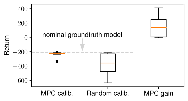
Figure 7: Swingup task cumulative reward (return) on 50 randomly sampled environment instances using a learned context-conditional model and an analytic reward function for planning. The learned model is conditioned on 30 transitions collected using the MPC calibration scheme or random sampling, respectively. "MPC gain" is gain in return when using MPC calibration scheme instead of random calibration. "Nominal groundtruth model" refers to the baseline performance when planning using groundtruth dynamics as forward model with $\alpha_{i}=1.25$.

4.4 MountainCar environment

(a) Sampled terrain profiles of the MountainCar environment.

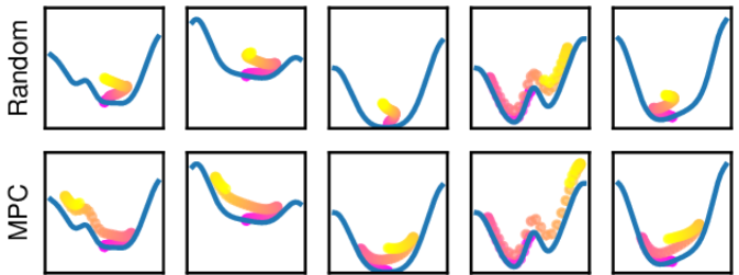
(b) Random (top) vs MPC (bottom) calibration rollouts on 5 sampled MountainCar profiles (pink: t=1, yellow: t=50). The MPC rollouts cover larger extents of the profile to infer its shape. For better visibility, rollouts are extruded over time towards the positive y-direction.

Figure 8: Properties of the MountainCar environment

The MountainCar environment was first introduced by Moore, (1990) and is a common benchmarking problem for reinforcement learning algorithms. In its original formulation, the task is to steer a car from a valley to a hill on a 2D profile. Due to throttle constraints on the car, the agent has to learn to gain momentum by first steering in the opposite direction of the goal. We extend the MountainCar environment to randomly sampled 2D terrain shapes, train context-conditional dynamics models on random rollouts and evaluate our proposed calibration routines. Figure 8(a) illustrates randomly sampled terrain profiles. The supplementary material provides further details on the environment.

Data collection

For data collection, we generate random rollouts on 60k MountainCar environment instances with randomly sampled terrain profiles.

Evaluation

All calibration rollouts contain 50 transitions and are initialized at $x_{0}=\dot{x}_{0}=0$. We depict the resulting random and MPC calibration rollouts in Figure 8(b). Similar to the Pendulum environment, the MPC calibration exhibits an explorative behavior to gain information about the terrain shape. The prediction error is evaluated on $50$ randomly sampled terrain profiles, $20$ randomly generated rollouts per profile and 3 independently trained models, giving 3000 rollouts in total. The model prediction error is depicted in Figure 4(b) for different calibration schemes. Again, our proposed calibration schemes compare favourably to using random transitions for calibration. The CEM planning horizon for MPC calibration for this environment is set to $H_{\mathrm{max}}=30$ in our experiments.

5 CONCLUSION

In this paper, we propose a learning method for context-dependent probabilistic dynamics models and an information-theoretic calibration approach to adapt the dynamics models to target environments from experience. We apply the framework of Neural Processes (Garnelo et al., 2018b, ) with a probabilistic context encoder to formulate our latent dynamics model and propose a learning approach that learns meaningful predictions of the uncertainty in the context variable. Our calibration approach uses expected information gain in the latent context variable as optimization criterion for model-predictive control. For evaluation, we construct an illustrative toy environment, on which we can easily distinct informative and non-informative actions for inferring a latent parameter. Experiments on this toy problem reveal the characteristics of the probabilistic encoding for informative and non-informative actions. We also introduce parameterized pendulum and mountain car environments to demonstrate our method on more complex systems. On the systems, our proposed calibration methods yield models with significantly lower prediction errors compared to random calibration. In future work, we plan to extend our method for learning dynamics models of real systems and for model-based control and reinforcement learning. Modelling partially observable environments also is an interesting avenue of future research.

Acknowledgements

This work has been supported by Cyber Valley and the Max Planck Society. The authors thank the International Max Planck Research School for Intelligent Systems (IMPRS-IS) for supporting Jan Achterhold. We thank the anonymous reviewers for their insightful comments.

References

- Brockman et al., (2016) Brockman, G., Cheung, V., Pettersson, L., Schneider, J., Schulman, J., Tang, J., and Zaremba, W. (2016). Openai gym. arXiv:1606.01540.
- Buisson-Fenet et al., (2020) Buisson-Fenet, M., Solowjow, F., and Trimpe, S. (2020). Actively learning gaussian process dynamics. In Proceedings of the 2nd Conference on Learning for Dynamics and Control (L4DC), volume 120 of Proceedings of Machine Learning Research, pages 5–15. PMLR.
- Chaloner and Verdinelli, (1995) Chaloner, K. and Verdinelli, I. (1995). Bayesian experimental design: A review. Statistical Science, 10(3):273–304.
- Cho et al., (2014) Cho, K., van Merrienboer, B., Gülçehre, Ç., Bahdanau, D., Bougares, F., Schwenk, H., and Bengio, Y. (2014). Learning phrase representations using RNN encoder-decoder for statistical machine translation. In Proceedings of the Conference on Empirical Methods in Natural Language Processing (EMNLP), pages 1724–1734. ACL.
- Chua et al., (2018) Chua, K., Calandra, R., McAllister, R., and Levine, S. (2018). Deep reinforcement learning in a handful of trials using probabilistic dynamics models. In Advances in Neural Information Processing Systems (NeurIPS), volume 31. Curran Associates, Inc.
- Deisenroth and Rasmussen, (2011) Deisenroth, M. and Rasmussen, C. (2011). PILCO: A model-based and data-efficient approach to policy search. In Proceedings of the 28th International Conference on Machine Learning (ICML), pages 465–472. Omnipress.
- Duan et al., (2016) Duan, Y., Schulman, J., Chen, X., Bartlett, P. L., Sutskever, I., and Abbeel, P. (2016). RL2: Fast reinforcement learning via slow reinforcement learning. CoRR, abs/1611.02779.
- Epshteyn et al., (2008) Epshteyn, A., Vogel, A., and DeJong, G. (2008). Active reinforcement learning. In Cohen, W. W., McCallum, A., and Roweis, S. T., editors, Proceedings of the International Conference on Machine Learning (ICML), volume 307 of ACM International Conference Proceeding Series, pages 296–303. ACM.
- Finn et al., (2017) Finn, C., Abbeel, P., and Levine, S. (2017). Model-agnostic meta-learning for fast adaptation of deep networks. In Proceedings of the International Conference on Machine Learning (ICML), volume 70 of Proceedings of Machine Learning Research, pages 1126–1135. PMLR.
- Foster et al., (2019) Foster, A., Jankowiak, M., Bingham, E., Horsfall, P., Teh, Y. W., Rainforth, T., and Goodman, N. D. (2019). Variational bayesian optimal experimental design. In Advances in Neural Information Processing Systems (NeurIPS), pages 14036–14047.
- Fraccaro et al., (2017) Fraccaro, M., Kamronn, S., Paquet, U., and Winther, O. (2017). A disentangled recognition and nonlinear dynamics model for unsupervised learning. In Advances in Neural Information Processing Systems (NeurIPS), pages 3601–3610.
- Franceschini and Macchietto, (2008) Franceschini, G. and Macchietto, S. (2008). Model-based design of experiments for parameter precision: State of the art. Chemical Engineering Science, 63(19):4846–4872.
- (13) Garnelo, M., Rosenbaum, D., Maddison, C., Ramalho, T., Saxton, D., Shanahan, M., Teh, Y. W., Rezende, D. J., and Eslami, S. M. A. (2018a). Conditional neural processes. In Proceedings of the International Conference on Machine Learning (ICML), volume 80 of Proceedings of Machine Learning Research, pages 1690–1699. PMLR.
- (14) Garnelo, M., Schwarz, J., Rosenbaum, D., Viola, F., Rezende, D. J., Eslami, S. M. A., and Teh, Y. W. (2018b). Neural processes. CoRR, abs/1807.01622.
- Golovin et al., (2010) Golovin, D., Krause, A., and Ray, D. (2010). Near-optimal bayesian active learning with noisy observations. In Advances in Neural Information Processing Systems (NeurIPS), pages 766–774.
- Hafner et al., (2019) Hafner, D., Lillicrap, T., Fischer, I., Villegas, R., Ha, D., Lee, H., and Davidson, J. (2019). Learning latent dynamics for planning from pixels. In Proceedings of the International Conference on Machine Learning (ICML), volume 97 of Proceedings of Machine Learning Research, pages 2555–2565. PMLR.
- Hafner et al., (2020) Hafner, D., Lillicrap, T. P., Ba, J., and Norouzi, M. (2020). Dream to control: Learning behaviors by latent imagination. In International Conference on Learning Representations (ICLR). OpenReview.net.
- Kingma and Ba, (2015) Kingma, D. P. and Ba, J. (2015). Adam: A method for stochastic optimization. In Proc. of the International Conference on Learning Representations (ICLR).
- Lindley, (1956) Lindley, D. V. (1956). On a measure of the information provided by an experiment. The Annals of Mathematical Statistics, 27(4):986–1005.
- MacKay, (1992) MacKay, D. J. C. (1992). Information-based objective functions for active data selection. Neural Comput., 4(4):590–604.
- Moore, (1990) Moore, A. (1990). Efficient Memory-based Learning for Robot Control. PhD thesis.
- Murphy, (2012) Murphy, K. P. (2012). Machine learning - a probabilistic perspective. Adaptive computation and machine learning series. MIT Press.
- Nagabandi et al., (2019) Nagabandi, A., Clavera, I., Liu, S., Fearing, R. S., Abbeel, P., Levine, S., and Finn, C. (2019). Learning to adapt in dynamic, real-world environments through meta-reinforcement learning. In International Conference on Learning Representations (ICLR). OpenReview.net.
- Roy and McCallum, (2001) Roy, N. and McCallum, A. (2001). Toward optimal active learning through monte carlo estimation of error reduction. In Proceedings of the International Conference on Machine Learning (ICML).
- Rubinstein, (1999) Rubinstein, R. (1999). The cross-entropy method for combinatorial and continuous optimization. Methodology And Computing In Applied Probability, 1(2):127–190.
- Sekar et al., (2020) Sekar, R., Rybkin, O., Daniilidis, K., Abbeel, P., Hafner, D., and Pathak, D. (2020). Planning to explore via self-supervised world models. In Proceedings of the International Conference on Machine Learning (ICML), Proceedings of Machine Learning Research, pages 8583–8592. PMLR.
- Shyam et al., (2019) Shyam, P., Jaskowski, W., and Gomez, F. (2019). Model-based active exploration. In Proceedings of the International Conference on Machine Learning (ICML), volume 97 of Proceedings of Machine Learning Research, pages 5779–5788. PMLR.
- Singh et al., (2019) Singh, G., Yoon, J., Son, Y., and Ahn, S. (2019). Sequential neural processes. In Advances in Neural Information Processing Systems (NeurIPS), pages 10254–10264.
- Sæmundsson et al., (2018) Sæmundsson, S., Hofmann, K., and Deisenroth, M. P. (2018). Meta reinforcement learning with latent variable gaussian processes. In Conference on Uncertainty in Artificial Intelligence (UAI).
- Tschantz et al., (2020) Tschantz, A., Millidge, B., Seth, A. K., and Buckley, C. L. (2020). Reinforcement learning through active inference. CoRR, abs/2002.12636.
- Watter et al., (2015) Watter, M., Springenberg, J., Boedecker, J., and Riedmiller, M. (2015). Embed to control: A locally linear latent dynamics model for control from raw images. In Advances in Neural Information Processing Systems (NeurIPS), pages 2746–2754. Curran Associates, Inc.
- Zaheer et al., (2017) Zaheer, M., Kottur, S., Ravanbakhsh, S., Póczos, B., Salakhutdinov, R., and Smola, A. J. (2017). Deep sets. In Advances in Neural Information Processing Systems (NeurIPS), pages 3391–3401.
- Zhu et al., (2020) Zhu, B., Wang, S., and Zhang, J. (2020). Neural physicist: Learning physical dynamics from image sequences. CoRR, abs/2006.05044.