MagNet: A Neural Network for Directed Graphs

Abstract

The prevalence of graph-based data has spurred the rapid development of graph neural networks (GNNs) and related machine learning algorithms. Yet, despite the many datasets naturally modeled as directed graphs, including citation, website, and traffic networks, the vast majority of this research focuses on undirected graphs. In this paper, we propose MagNet, a spectral GNN for directed graphs based on a complex Hermitian matrix known as the magnetic Laplacian. This matrix encodes undirected geometric structure in the magnitude of its entries and directional information in their phase. A “charge” parameter attunes spectral information to variation among directed cycles. We apply our network to a variety of directed graph node classification and link prediction tasks showing that MagNet performs well on all tasks and that its performance exceeds all other methods on a majority of such tasks. The underlying principles of MagNet are such that it can be adapted to other spectral GNN architectures.

1 Introduction

Endowing a collection of objects with a graph structure allows one to encode pairwise relationships among its elements. These relations often possess a natural notion of direction. For example, the WebKB dataset [32] contains a list of university websites with associated hyperlinks. In this context, one website might link to a second without a reciprocal link to the first. Such datasets are naturally modeled by directed graphs. In this paper, we introduce MagNet, a graph convolutional neural network for directed graphs based on the magnetic Laplacian.

Most graph neural networks fall into one of two families, spectral networks or spatial networks. Spatial methods define graph convolution as a localized averaging operation with iteratively learned weights. Spectral networks, on the other hand, define convolution on graphs via the eigendecompositon of the (normalized) graph Laplacian. The eigenvectors of the graph Laplacian assume the role of Fourier modes, and convolution is defined as entrywise multiplication in the Fourier basis. For a comprehensive review of both spatial and spectral networks, we refer the reader to [42] and [40].

Many spatial graph CNNs have natural extensions to directed graphs. However, it is common for these methods to preprocess the data by symmetrizing the adjacency matrix, effectively creating an undirected graph. For example, while [38] explicitly notes that their network is well-defined on directed graphs, their experiments treat all citation networks as undirected for improved performance.

Extending spectral methods to directed graphs is not straightforward since the adjacency matrix is asymmetric and, thus, there is no obvious way to define a symmetric, real-valued Laplacian with a full set of real eigenvalues that uniquely encodes any directed graph. We overcome this challenge by constructing a network based on the magnetic Laplacian $\mathbf{L}^{(q)}$ defined in Section 2. Unlike the directed graph Laplacians used in works such as [26, 30, 36, 37], the magnetic Laplacian is not a real-valued symmetric matrix. Instead, it is a complex-valued Hermitian matrix that encodes the fundamentally asymmetric nature of a directed graph via the complex phase of its entries.

Since $\mathbf{L}^{(q)}$ is Hermitian, the spectral theorem implies it has an orthonormal basis of complex eigenvectors corresponding to real eigenvalues. Moreover, Theorem 1, stated in Appendix E, shows that $\mathbf{L}^{(q)}$ is positive semidefinite, similar to the traditional Laplacian. Setting $q=0$ is equivalent to symmetrizing the adjacency matrix and no importance is given to directional information. When $q=.25$, on the other hand, we have that $\mathbf{L}^{(.25)}(u,v)=-\mathbf{L}^{(.25)}(v,u)$ whenever there is an edge from $u$ to $v$ but not from $v$ to $u$. Different values of $q$ highlight different graph motifs [16, 17, 19, 29], and therefore the optimal choice of $q$ varies. Learning the appropriate value of $q$ from data allows MagNet to adaptively incorporate directed information. We also note that $\mathbf{L}^{(q)}$ has been applied to graph signal processing [18], community detection [17], and clustering [10, 16, 15].

In Section 3, we show how the networks constructed in [6, 13, 22] can be adapted to directed graphs by incorporating complex Hermitian matrices, such as the magnetic Laplacian. When $q=0$, we effectively recover the networks constructed in those previous works. Therefore, our work generalizes these networks in a way that is suitable for directed graphs. Our method is very general and is not tied to any particular choice of network architecture. Indeed, the main ideas of this work could be adapted to nearly any spectral network.

In Section 4, we summarize related work on directed graph neural networks as well as other papers studying the magnetic Laplacian and its applications in data science. In Section 5, we apply our network to node classification and link prediction tasks. We compare against several spectral and spatial methods as well as networks designed for directed graphs. We find that MagNet obtains the best or second-best performance on five out of six node-classification tasks and has the best performance on seven out of eight link-prediction tasks tested on real-world data, in addition to providing excellent node-classification performance on difficult synthetic data. In the appendix, we provide full implementation details, theoretical results concerning the magnetic Laplacian, extended examples, and further numerical details.

2 The magnetic Laplacian

Spectral graph theory has been remarkably successful in relating geometric characteristics of undirected graphs to properties of eigenvectors and eigenvalues of graph Laplacians and related matrices. For example, the tasks of optimal graph partitioning, sparsification, clustering, and embedding may be approximated by eigenvectors corresponding to small eigenvalues of various Laplacians (see, e.g., [9, 34, 2, 35, 11]). Similarly, the graph signal processing research community leverages the full set of eigenvectors to extend the Fourier transform to these structures [31]. Furthermore, numerous papers [6, 13, 22] have shown that this eigendecomposition can be used to define neural networks on graphs. In this section, we provide the background needed to extend these constructions to directed graphs via complex Hermitian matrices such as the magnetic Laplacian.

We let $G=(V,E)$ be a directed graph where $V$ is a set of $N$ vertices and $E\subseteq V\times V$ is a set of directed edges. If $(u,v)\in E$, then we say there is an edge from $u$ to $v$. For the sake of simplicity, we will focus on the case where the graph is unweighted and has no self-loops, i.e., $(v,v)\notin E$, but our methods have natural extensions to graphs with self-loops and/or weighted edges. If both $(u,v)\in E$ and $(v,u)\in E$, then one may consider this pair of directed edges as a single undirected edge.

A directed graph can be described by an adjacency matrix $(\mathbf{A}(u,v))_{u,v\in V}$ where $\mathbf{A}(u,v)=1$ if $(u,v)\in E$ and $\mathbf{A}(u,v)=0$ otherwise. Unless $G$ is undirected, $\mathbf{A}$ is not symmetric, and, indeed, this is the key technical challenge in extending spectral graph neural networks to directed graphs. In the undirected case, where the adjacency matrix $\mathbf{A}$ is symmetric, the (unnormalized) graph Laplacian can be defined by $\mathbf{L}=\mathbf{D}-\mathbf{A},$ where $\mathbf{D}$ is a diagonal degree matrix. It is well-known that $\mathbf{L}$ is a symmetric, positive-semidefinite matrix and therefore has an orthonormal basis of eigenvectors associated with non-negative eigenvalues. However, when $\mathbf{A}$ is asymmetric, direct attempts to define the Laplacian this way typically yield complex eigenvalues. This impedes the straightforward extension of classical methods of spectral graph theory and graph signal processing to directed graphs.

A key point of this paper is to represent the directed graph through a complex Hermitian matrix $\bm{\mathcal{L}}$ such that: (1) the magnitude of $\bm{\mathcal{L}}(u,v)$ indicates the presence of an edge, but not its direction; and (2) the phase of $\bm{\mathcal{L}}(u,v)$ indicates the direction of the edge, or if the edge is undirected. Such matrices have been explored in the directed graph literature (see Section 4), but not in the context of graph neural networks. They have several advantages over their real-valued matrix counterparts. In particular, a single symmetric real-valued matrix will not uniquely represent a directed graph. Instead, one must use several matrices, as in [37], but this increases the complexity of the resulting network. Alternatively, one can work with an asymmetric, real-valued matrix, such as the adjacency matrix or the random walk matrix. However, the spatial graph filters that result from such matrices are typically limited by the fact that they can only aggregate information from the vertices that can be reached in one hop from a central vertex, but ignore the equally important subset of vertices that can reach the central vertex in one hop. Complex Hermitian matrices, however, lead to filters that aggregate information from both sets of vertices. Finally, one could use a real-valued skew-symmetric matrix but such matrices do not generalize well to graphs with both directed and undirected edges.

The optimal choice of complex Hermitian matrix is an open question. Here, we utilize a parameterized family of magnetic Laplacians, which have proven to be useful in other data-driven contexts [17, 10, 16, 15]. We first define the symmetrized adjacency matrix and corresponding degree matrix by,

$$\mathbf{A}_{s}(u,v)\coloneqq\frac{1}{2}(\mathbf{A}(u,v)+\mathbf{A}(v,u)),\,\>\>1\leq u,v\leq N,\quad\mathbf{D}_{s}(u,u)\coloneqq\sum_{v\in V}\mathbf{A}_{s}(u,v),\>\>1\leq u\leq N\,,$$

with $\mathbf{D}_{s}(u,v)=0$ for $u\neq v$. We capture directional information via a phase matrix, $\bm{\Theta}^{(q)}$,

$$\bm{\Theta}^{(q)}(u,v)\coloneqq 2\pi q(\mathbf{A}(u,v)-\mathbf{A}(v,u))\,,\quad q\geq 0\,,$$

where $\exp(i\bm{\Theta}^{(q)})$ is defined component-wise by $\exp(i\bm{\Theta}^{(q)})(u,v)\coloneqq\exp(i\bm{\Theta}^{(q)}(u,v))$. Letting $\odot$ denotes componentwise multiplication, we define the complex Hermitian adjacency matrix $\mathbf{H}^{(q)}$ by

$$\mathbf{H}^{(q)}\coloneqq\mathbf{A}_{s}\odot\exp(i\bm{\Theta}^{(q)})\,.$$

Since $\bm{\Theta}^{(q)}$ is skew-symmetric, $\mathbf{H}^{(q)}$ is Hermitian. When $q=0$, we have $\bm{\Theta}^{(0)}=\bm{0}$ and so $\mathbf{H}^{(0)}=\mathbf{A}_{s}$. This effectively corresponds to treating the graph as undirected. For $q\neq 0$, the phase of $\mathbf{H}^{(q)}$ encodes edge direction. For example, if there is an edge from $u$ to $v$ but not from $v$ to $u$ we have

$$\mathbf{H}^{(.25)}(u,v)=\frac{i}{2}=-\mathbf{H}^{(.25)}(v,u)\,.$$

Thus, in this setting, an edge from $u$ to $v$ is treated as the opposite of an edge from $v$ to $u$. On the other hand, if $(u,v),(v,u)\in E$ (which can be interpreted as a single undirected edge), then $\mathbf{H}^{(q)}(u,v)=\mathbf{H}^{(q)}(v,u)=1$, and we see the phase, $\bm{\Theta}^{(q)}(u,v)=0$, encodes the lack of direction in the edge. For the rest of this paper, we will assume that $q$ lies in between these two extreme values, i.e., $0\leq q\leq.25.$ We define the normalized and unnormalized magnetic Laplacians by

$$\mathbf{L}_{U}^{(q)}\coloneqq\mathbf{D}_{s}-\mathbf{H}^{(q)}=\mathbf{D}_{s}-\mathbf{A}_{s}\odot\exp(i\bm{\Theta}^{(q)}),\quad\mathbf{L}_{N}^{(q)}\coloneqq\mathbf{I}-\left(\mathbf{D}_{s}^{-1/2}\mathbf{A}_{s}\mathbf{D}_{s}^{-1/2}\right)\odot\exp(i\bm{\Theta}^{(q)})\,.$$ (1)

Note that when $G$ is undirected, $\mathbf{L}_{U}^{(q)}$ and $\mathbf{L}_{N}^{(q)}$ reduce to the standard undirected Laplacians.

$\mathbf{L}_{U}^{(q)}$ and $\mathbf{L}_{N}^{(q)}$ are Hermitian. Theorem 1 (see Appendix E) shows they are positive-semidefinite and thus are diagonalized by an orthonormal basis of complex eigenvectors $\mathbf{u}_{1},\ldots,\mathbf{u}_{N}$ associated to real, nonnegative eigenvalues $\lambda_{1},\ldots,\lambda_{N}$. Similar to the traditional normalized Laplacian, Theorem 2 (see Appendix E) shows that the eigenvalues of $\mathbf{L}^{q}_{N}$ lie in $[0,2]$, and we may factor $\mathbf{L}_{N}^{(q)}=\mathbf{U}\bm{\Lambda}\mathbf{U}^{\dagger}$, where $\mathbf{U}$ is the $N\times N$ matrix whose $k$-th column is $\mathbf{u}_{k}$, $\bm{\Lambda}$ is the diagonal matrix with $\bm{\Lambda}(k,k)=\lambda_{k}$, and $\mathbf{U}^{\dagger}$ is the conjugate transpose of $\mathbf{U}$ (a similar formula holds for $\mathbf{L}^{(q)}_{U}$). The magnetic Laplacian encodes geometric information in its eigenvectors and eigenvalues. In the directed star graph (see Appendix F), for example, directional information is contained in the eigenvectors only, whereas the eigenvalues are invariant to the direction of the edges. On the other hand, for the directed cycle graph the magnetic Laplacian encodes the directed nature of the graph solely in its spectrum. In general, both the eigenvectors and eigenvalues may contain important information. In Section 3, we will introduce MagNet, a network designed to leverage this spectral information.

3 MagNet

Most graph neural network architectures can be described as being either spectral or spatial. Spatial networks such as [38, 20, 1, 14] typically extend convolution to graphs by performing a weighted average of features over neighborhoods $\mathcal{N}(u)=\{v:(u,v)\in{E}\}$. These neighborhoods are well-defined even when ${E}$ is not symmetric, so spatial methods typically have natural extensions to directed graphs. However, such simplistic extensions may miss important information in the directed graph. For example, filters defined using $\mathcal{N}(u)$ are not capable of assimilating the equally important information contained in $\{v:(v,u)\in E\}$. Alternatively, these methods may also use the symmetrized adjacency matrix, but they cannot learn to balance directed and undirected approaches.

In this section, we show how to extend spectral methods to directed graphs using the magnetic Laplacian introduced in Section 2. To highlight the flexibility of our approach, we show how three spectral graph neural network architectures can be adapted to incorporate the magnetic Laplacian. Our approach is very general, and so for most of this section, we will perform our analysis for a general complex Hermitian, positive semidefinite matrix. However, we view the magnetic Laplacian as our primary object of interest (and use it in all of our experiments in Section 5) because of the large body of literature studying its spectral properties and applying it to data science (see Section 4).

3.1 Spectral convolution via the magnetic Laplacian

In this section, we let $\bm{\mathcal{L}}$ denote a Hermitian, positive semidefinite matrix, such as the normalized or unnormalized magnetic Laplacian introduced in Section 2, on a directed graph $G=(V,E)$, $|V|=N$. We let $\mathbf{u}_{1}\ldots,\mathbf{u}_{N}$ be an orthonormal basis of eigenvectors for $\bm{\mathcal{L}}$ and let $\mathbf{U}$ be the $N\times N$ matrix whose $k$-th column is $\mathbf{u}_{k}$. We define the directed graph Fourier transform for a signal $\mathbf{x}:V\rightarrow\mathbb{C}$ by $\widehat{\mathbf{x}}=\mathbf{U}^{\dagger}\mathbf{x}$, so that $\widehat{\mathbf{x}}(k)=\langle\mathbf{x},\mathbf{u}_{k}\rangle\,.$ We regard the eigenvectors $\mathbf{u}_{1},\ldots,\mathbf{u}_{N}$ as the generalizations of discrete Fourier modes to directed graphs. Since $\mathbf{U}$ is unitary, we have the Fourier inversion formula

$$\mathbf{x}=\mathbf{U}\widehat{\mathbf{x}}=\sum_{k=1}^{N}\widehat{\mathbf{x}}(k)\mathbf{u}_{k}\,.$$ (2)

In Euclidean space, convolution corresponds to pointwise multiplication in the Fourier basis. Thus, we define the convolution of $\mathbf{x}$ with a filter $\mathbf{y}$ in the Fourier domain by $\widehat{\mathbf{y}\ast\mathbf{x}}(k)=\widehat{\mathbf{y}}(k)\widehat{\mathbf{x}}(k)$. By (2), this implies $\mathbf{y}\ast\mathbf{x}=\mathbf{U}\text{Diag}(\widehat{\mathbf{y}})\widehat{\mathbf{x}}=(\mathbf{U}\text{Diag}(\widehat{\mathbf{y}})\mathbf{U}^{\dagger})\mathbf{x}$, and so we say $\mathbf{Y}$ is a convolution matrix if

$$\mathbf{Y}=\mathbf{U}\bm{\Sigma}\mathbf{U}^{\dagger}\,,$$ (3)

for a diagonal matrix $\bm{\Sigma}.$ This is the natural generalization of the class of convolutions used in [6].

Next, following [13] (see also [21]), we show that a spectral network can be implemented in the spatial domain via polynomials of $\bm{\mathcal{L}}$ by having $\bm{\Sigma}$ be a polynomial of $\bm{\Lambda}$ in (3). This reduces the number of trainable parameters to prevent overfitting, avoids explicit diagonalization of the matrix $\bm{\mathcal{L}}$, (which is expensive for large graphs), and improves stability to perturbations [24]. As in [13], we define a normalized eigenvalue matrix, with entries in $[-1,1]$, by $\widetilde{\bm{\Lambda}}=\frac{2}{\lambda_{\max}}\bm{\Lambda}-\mathbf{I}$ and assume

$$\bm{\Sigma}=\sum_{k=0}^{K}\theta_{k}T_{k}(\widetilde{\bm{\Lambda}})\,,$$

for some real-valued $\theta_{1},\ldots,\theta_{k},$ where for $k\geq 0$, $T_{k}$ is the Chebyshev polynomial defined by $T_{0}(x)=1,T_{1}(x)=x,$ and $T_{k}(x)=2xT_{k-1}(x)+T_{k-2}(x)$ for $k\geq 2.$ One can use the fact that $(\mathbf{U}\widetilde{\bm{\Lambda}}\mathbf{U}^{\dagger})^{k}=\mathbf{U}\widetilde{\bm{\Lambda}}^{k}\mathbf{U}^{\dagger}$ to see

$$\mathbf{Y}\mathbf{x}=\mathbf{U}\sum_{k=0}^{K}\theta_{k}T_{k}(\widetilde{\bm{\Lambda}})\mathbf{U}^{\dagger}\mathbf{x}=\sum_{k=0}^{K}\theta_{k}T_{k}(\widetilde{\bm{\mathcal{L}}})\mathbf{x}\,,$$ (4)

where, analogous to $\widetilde{\bm{\Lambda}}$, we define $\widetilde{\bm{\mathcal{L}}}\coloneqq\frac{2}{\lambda_{\text{max}}}\bm{\mathcal{L}}-\mathbf{I}$. It is important to note that, due to the complex Hermitian structure of $\widetilde{\bm{\mathcal{L}}}$, the value $\mathbf{Y}\mathbf{x}(u)$ aggregates information both from the values of $\mathbf{x}$ on $\mathcal{N}_{k}(u)$, the $k$-hop neighborhood of $u$, and the values of $\mathbf{x}$ on $\{v:\mathrm{dist}(v,u)\leq k\}$, which consists of those of vertices that can reach $u$ in $k$-hops. While in an undirected graph these two sets of vertices are the same, that is not the case for general directed graphs. Furthermore, due to the difference in phase between an edge $(u,v)$ and an edge $(v,u)$, the filter matrix $\mathbf{Y}$ is also capable of aggregating information from these two sets in different ways. This capability is in contrast to any single, symmetric, real-valued matrix, as well as any matrix that encodes just $\mathcal{N}(u)$.

To obtain a network similar to [22], we set $K=1$, assume that $\bm{\mathcal{L}}=\mathbf{L}^{(q)}_{N}$, using $\lambda_{\max}\leq 2$ (see Theorem 2 in Appendix E) make the approximation $\lambda_{\max}\approx 2$, and set $\theta_{1}=-\theta_{0}.$ With this, we obtain

$$\mathbf{Y}\mathbf{x}=\theta_{0}(\mathbf{I}+(\mathbf{D}_{s}^{-1/2}\mathbf{A}_{s}\mathbf{D}_{s}^{-1/2})\odot\exp(i\bm{\Theta}^{(q)}))\mathbf{x}\,.$$

As in [22], we substitute $(\mathbf{I}+(\mathbf{D}_{s}^{-1/2}\mathbf{A}_{s}\mathbf{D}_{s}^{-1/2})\odot\exp(i\bm{\Theta}^{(q)})\rightarrow\widetilde{\mathbf{D}}_{s}^{-1/2}\widetilde{\mathbf{A}}_{s}\widetilde{\mathbf{D}}_{s}^{-1/2}\exp(i\bm{\Theta}^{(q)}).$ This renormalization helps avoid instabilities arising from vanishing/exploding gradients and yields

$$\mathbf{Y}\mathbf{x}=\theta_{0}\widetilde{\mathbf{D}}_{s}^{-1/2}\widetilde{\mathbf{A}}_{s}\widetilde{\mathbf{D}}_{s}^{-1/2}\odot\exp(i\bm{\Theta}^{(q)})\,,$$ (5)

where $\widetilde{\mathbf{A}}_{s}=\mathbf{A}_{s}+\mathbf{I}$ and $\widetilde{\mathbf{D}}_{s}(i,i)=\sum_{j}\widetilde{\mathbf{A}}_{s}(i,j)$.

3.2 The MagNet architecture

We now define our network. Let $L$ be the number of convolution layers in our network, and let $\mathbf{X}^{(0)}$ be an $N\times F_{0}$ input feature matrix with columns $\mathbf{x}^{(0)}_{1},\ldots\mathbf{x}^{(0)}_{F_{0}}$. Since our filters are complex, we use a complex version of ReLU defined by $\sigma(z)=z$, if $-\pi/2\leq\arg(z)<\pi/2$, and $\sigma(z)=0$ otherwise (where $\arg(z)$ is the complex argument of $z\in\mathbb{C}$). We let $F_{\ell}$ be the number of channels in layer $\ell$, and for $1\leq\ell\leq L$, $1\leq i\leq F_{\ell-1}$, and $1\leq j\leq F_{\ell},$ we let $\mathbf{Y}^{(\ell)}_{ij}$ be a convolution matrix defined in the sense of either (3), (4), or (5). To obtain the layer $\ell$ channels from the layer $\ell-1$ channels, we define the matrix $\mathbf{X}^{(\ell)}$ with columns $\mathbf{x}^{(\ell)}_{1},\ldots\mathbf{x}^{(\ell)}_{F_{\ell}}$ as:

$$\mathbf{x}^{(\ell)}_{j}=\sigma\left(\sum_{i=1}^{F_{\ell-1}}\mathbf{Y}_{ij}^{(\ell)}\mathbf{x}^{(\ell-1)}_{i}\right).$$ (6)

In matrix form we write $\mathbf{X}^{(\ell)}=\mathbf{Z}^{(\ell)}\left(\mathbf{X}^{(\ell-1)}\right)$, where $\mathbf{Z}^{(\ell)}$ is a hidden layer of the form (6).

After the convolutional layers, we unwind the complex $N\times F_{L}$ matrix $\mathbf{X}^{(L)}$ into a real-valued $N\times 2F_{L}$ matrix, apply a linear layer, consisting of right-multiplication by a $2F_{L}\times n_{c}$ weight matrix $\mathbf{W}^{(L+1)}$ (where $n_{c}$ is the number of classes) and apply softmax. In our experiments, we set $L=2$ or $3$. When $L=2$, our network applied to node classification, as illustrated in Figure 1, is given by

$$\text{softmax}(\text{unwind}(\mathbf{Z}^{(2)}(\mathbf{Z}^{(1)}(\mathbf{X}^{(0)})))\mathbf{W}^{\mathrm{(3)}})\,.$$

For link-prediction, we apply the same method through the unwind layer, and then concatenate the rows corresponding to pairs of nodes to obtain the edge features.

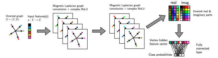
Figure 1: MagNet ($L=2$) applied to node classification. After two complex convolutional layers, we unwind the real and imaginary parts of our feature matrix and apply a fully connected layer.

4 Related work

In Section 4.1, we describe other graph neural networks designed specifically for directed graphs. Notably, none of these methods encode directionality with complex numbers, instead opting for real-valued, symmetric matrices. In Section 4.2, we review other work studying the magnetic Laplacian which has been studied for several decades and lately has garnered interest in the network science and graph signal processing communities. However, to the best of our knowledge, this is the first work to use it to construct a graph neural network. We also note there are numerous approaches to graph signal processing on directed graphs. Many of these rely on a natural analog of Fourier modes. These Fourier modes are typically defined through either a factorization of a graph shift operator or by solving an optimization problem. For further review, we refer the reader to [27].

4.1 Neural networks for directed graphs

In [26], the authors construct a directed Laplacian, via identities involving the random walk matrix and its stationary distribution $\bm{\Pi}$. When $G$ is undirected, one can use the fact that $\bm{\Pi}$ is proportional to the degree vector to verify this directed Laplacian reduces to the standard normalized graph Laplacian. However, this method requires $G$ to be strongly connected, unlike MagNet. The authors of [37] use a first-order proximity matrix $\mathbf{A}_{F}$ (equivalent to $\mathbf{A}_{s}$ here), as well as two second-order proximity matrices $\mathbf{A}_{S_{\text{in}}}$ and $\mathbf{A}_{S_{\text{out}}}$. $\mathbf{A}_{S_{\text{in}}}$ is defined by $\mathbf{A}_{S_{\text{in}}}(u,v)\neq 0$ if there exists a $w$ such that $(w,u),(w,v)\in E$, and $\mathbf{A}_{S_{\text{out}}}$ is defined analogously. These three matrices collectively describe and distinguish the neighborhood of each vertex and those vertices that can reach a vertex in a single hop. The authors construct three different Laplacians and use a fusion operator to share information across channels. Similarly, inspired by [3], in [30], the authors consider several different symmetric Laplacian matrices corresponding to a number of different graph motifs.

The method of [36] builds upon the ideas of both [26] and [37] and considers a directed Laplacian similar to the one used in [26], but with a PageRank matrix in place of the random-walk matrix. This allows for applications to graphs which are not strongly connected. Similar to [37], they use higher-order receptive fields (analogous to the second-order adjacency matrices discussed above) and an inception module to share information between receptive fields of different orders. We also note [23], which uses an approach based on PageRank in the spatial domain.

4.2 Related work on the magnetic Laplacian and Hermitian adjacency matrices

The magnetic Laplacian has been studied since at least [25]. The name originates from its interpretation as a quantum mechanical Hamiltonian of a particle under magnetic flux. Early works focused on $d$-regular graphs, where the eigenvectors of the magnetic Laplacian are equivalent to those of the Hermitian adjacency matrix. The authors of [19], for example, show that using a complex-valued Hermitian adjacency matrix rather than the symmetrized adjacency matrix reduces the number of small, non-isomorphic cospectral graphs. Topics of current research into Hermitian adjacency matrices include clustering tasks [12] and the role of the parameter $q$ [29].

The magnetic Laplacian is also the subject of ongoing research in graph signal processing [18], community detection [17], and clustering [10, 16, 15]. For example, [16] uses the phase of the eigenvectors to construct eigenmap embeddings analogous to [2]. The role of $q$ is highlighted in the works of [16, 17, 19, 29], which show how particular choices of $q$ may highlight various graph motifs. In our context, this indicates that $q$ should be carefully tuned via cross-validation. Lastly, we note that numerous other directed graph Laplacians have been studied and applied to data science [7, 8, 39]. However, as alluded to in Section 2, these methods typically do not use complex Hermitian matrices.

5 Numerical experiments

We test the performance of MagNet for node classification and link prediction on a variety of benchmark datasets as well as a directed stochastic block model.

5.1 Datasets

5.1.1 Directed Stochastic Block Model

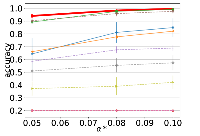
(a) Ordered DSBM with varying edge density.

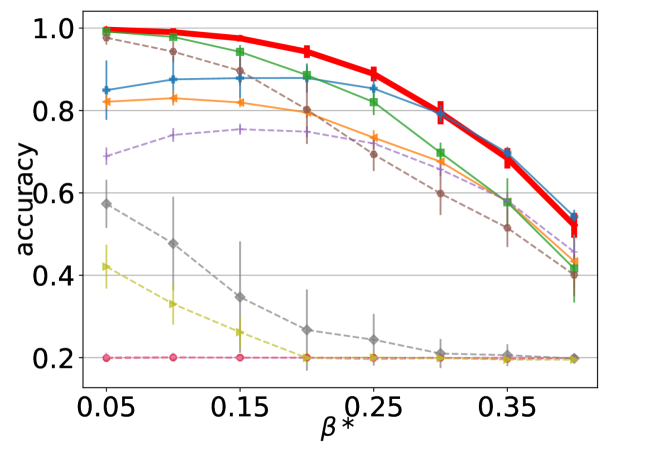
(b) Ordered DSBM with varying net flow.

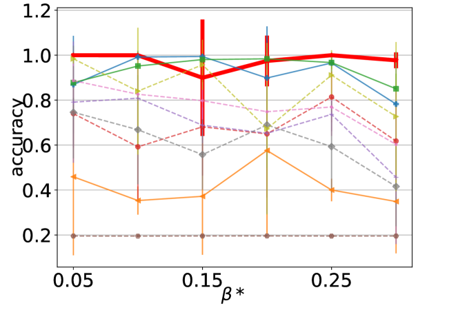
(c) Cyclic DSBM with varying net flow.

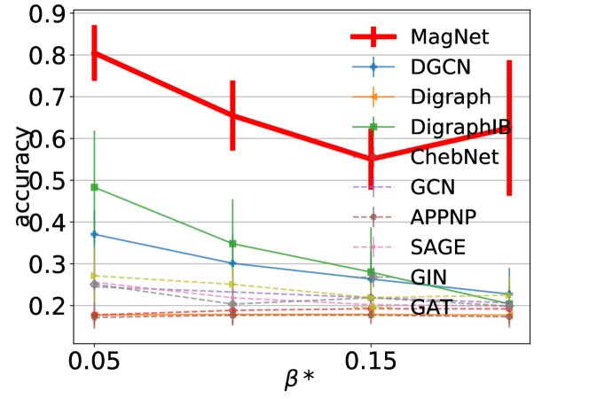
(d) Noisy Cyclic DSBM with varying net flow.

Figure 2: Node classification accuracy. Error bars are one standard error. MagNet is bold red.

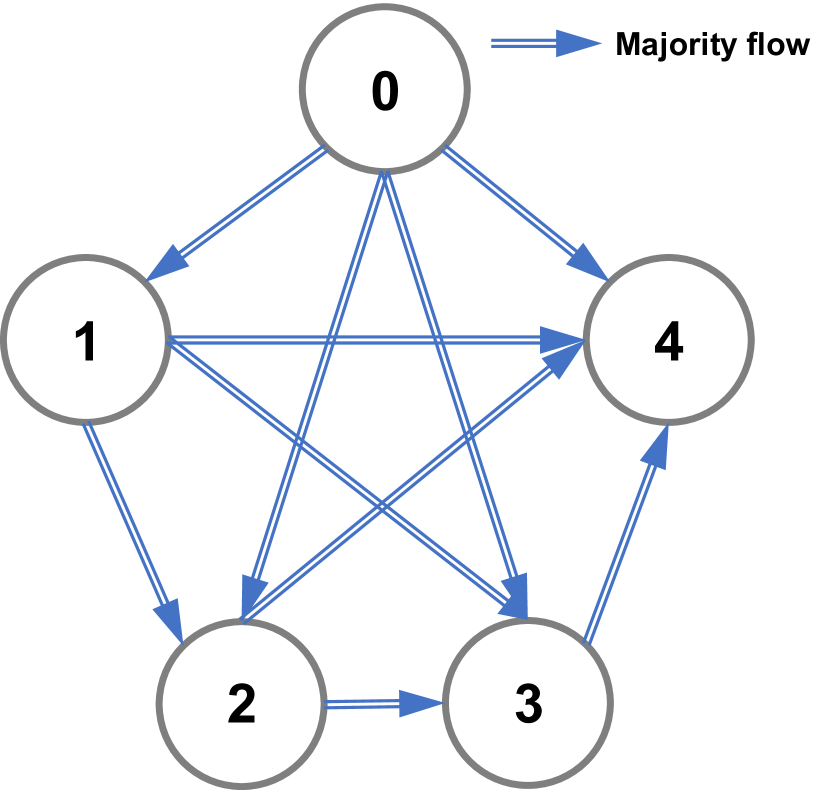
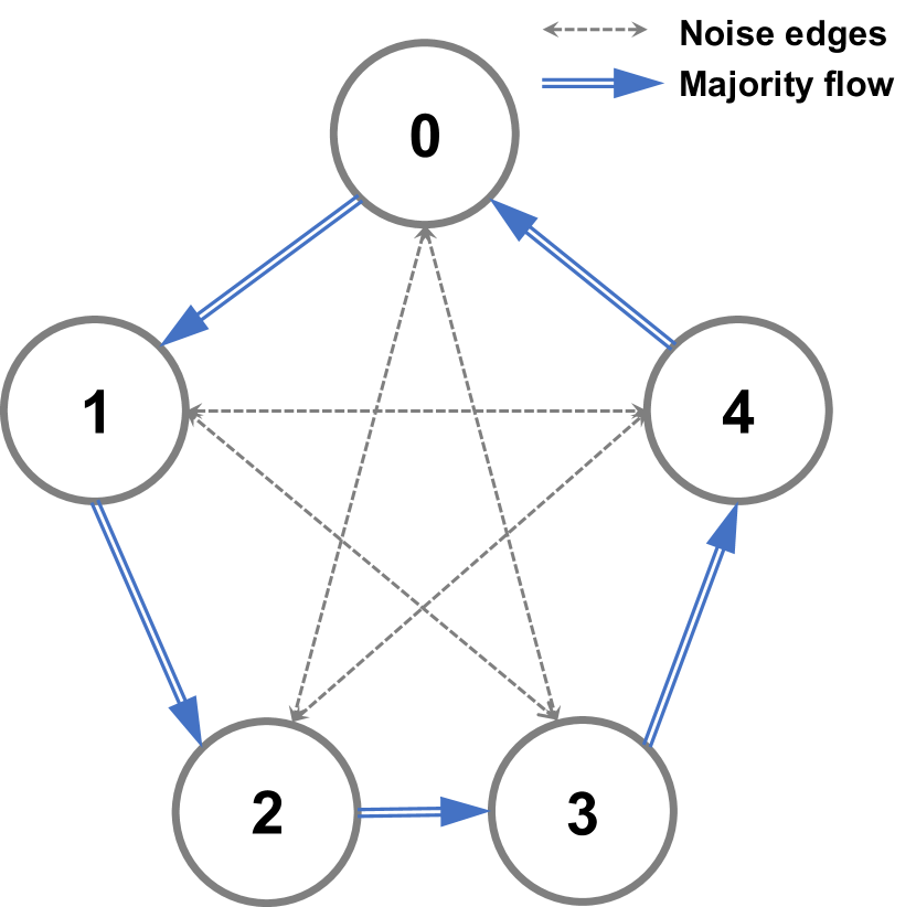
(e) Ordered meta-graph.

(f) Cyclic meta-graph.

Figure 3: Meta-graphs for the synthetic data sets.

We construct a directed stochastic block (DSBM) model as follows. First we divide $N$ vertices into $n_{c}$ equally-sized clusters $C_{1},\ldots,C_{n_{c}}$. We define $\{\alpha_{i,j}\}_{1\leq i,j\leq n_{c}}$ to be a collection of probabilities, $0<\alpha_{i,j}\leq 1$ with $\alpha_{i,j}=\alpha_{j,i}$, and for an unordered pair $u\neq v$ create an undirected edge between $u$ and $v$ with probability $\alpha_{i,j}$ if $u\in C_{i},v\in C_{j}$. To turn this undirected graph into a directed graph, we next define $\{\beta_{i,j}\}_{1\leq i,j\leq n_{c}}$ to be a collection of probabilities such that $0\leq\beta_{i,j}\leq 1$ and $\beta_{i,j}+\beta_{j,i}=1$. For each undirected edge $\{u,v\}$, we assign that edge a direction by the rule that the edge points from $u$ to $v$ with probability $\beta_{i,j}$ if $u\in C_{i}$ and $v\in C_{j}$, and points from $v$ to $u$ otherwise. We note that if $\alpha_{i,j}$ is constant, then the only way to determine the clusters will be from the directional information.

In Figure 2, we plot the performance of MagNet and other methods on variations of the DSBM. In each of these, we set $n_{c}=5$ and the goal is to classify the vertices by cluster. We set $N=2500$, except in Figure 2(d) where $N=500$. In Figure 2(a), we plot the performance of our model on the DSBM with $\alpha_{i,j}\coloneqq\alpha^{*}=.1,.08$, and $.05$ for $i\neq j$, which varies the density of inter-cluster edges, and set $\alpha_{i,i}=.1$. Here we set $\beta_{i,i}=.5$ and $\beta_{i,j}=.05$ for $i>j$. This corresponds to the ordered meta-graph in Figure 3. Figure 2(b) also uses the ordered meta-graph, but here we fix $\alpha_{i,j}=.1$ for all $i,j$, and set $\beta_{i,j}=\beta^{*},$ for $i>j$, and allow $\beta^{*}$ to vary from .05 to .4, which varies the net flow from one cluster to another. The results in Figure 2(c) utilize a cyclic meta-graph structure as in Figure 3 (without the gray noise edges). Specifically, we set $\alpha_{i,j}=.1$ if $i=j$ or $i=j\pm 1\mod 5$ and $\alpha_{i,j}=0$ otherwise. We define $\beta_{i,j}=\beta^{*}$, $\beta_{j,i}=1-\beta^{*}$ when $j=(i-1)\mod 5$, and $\beta_{i,j}=0$ otherwise. In Figure 2(d) we add noise to the cyclic structure of our meta-graph by setting $\alpha_{i,j}=.1$ for all $i,j$ and $\beta_{i,j}=.5$ for all $(i,j)$ connected by a gray edge in Figure 3 (keeping $\beta_{i,j}$ the same as in Figure 2(c) for the blue edges).

5.1.2 Real datasets

Texas, Wisconsin, and Cornell are WebKB datasets modeling links between websites at different universities [32]. We use these datasets for both link prediction and node classification with nodes labeled as student, project, course, staff, and faculty in the latter case. Telegram [5] is a pairwise influence network between $245$ Telegram channels with $8,912$ links. To the best of our knowledge, this dataset has not previously been studied in the graph neural network literature. Labels are generated from the method discussed in [5], with a total of four classes. The datasets Chameleon and Squirrel [33] represent links between Wikipedia pages related to chameleons and squirrels. We use these datasets for link prediction. Likewise, WikiCS [28] is a collection of Computer Science articles, which we also use for link prediction (see the tables in Appendix G). Cora-ML and CiteSeer are popular citation networks with node labels corresponding to scientific subareas. We use the versions of these datasets provided in [4]. Further details are given in the Appendix D.

5.2 Training and implementation details

Node classification is performed in a semi-supervised setting (i.e., access to the test data, but not the test labels, during training). For the datasets Cornell, Texas, Wisconsin, and Telegram we use a 60%/20%/20% training/validation/test split, which might be viewed as more akin to supervised learning, because of the small graph size. For Cora-ML and CiteSeer, we use the same split as [36]. For all of these datasets we use 10 random data splits. For the DSBM datasets, we generated 5 graphs randomly for each type and for each set of parameters, each with 10 different random node splits. We use $20\%$ of the nodes for validation and we vary the proportion of training samples based on the classification difficulty, using 2%, 10%, and 60% of nodes per class for the ordered, cyclic, and noisy cyclic DSBM graphs, respectively, during training, and the rest for testing. Hyperpameters were selected using one of the five generated graphs, and then applied to the other four generated graphs.

In the main text, there are two types of link prediction tasks conducted for performance evaluation. The first type is to predict the edge direction of pairs of vertices $u,v$ for which either $(u,v)\in E$ or $(v,u)\in E$. The second type is existence prediction. The model is asked to predict if $(u,v)\in E$ by considering ordered pairs of vertices $(u,v)$. For both types of link prediction, we removed 15% of edges for testing, 5% for validation, and use the rest of the edges for training. The connectivity was maintained during splitting. 10 splits were generated randomly for each graph and the input features are in-degree and out-degree of nodes. In the appendix, we report on two additional link prediction tasks based on a three-class classification setup: $(u,v)\in E$, $(v,u)\in E$, or $(u,v),(v,u)\notin E$. Full details are provided in Appendix D.

In all experiments, we used the normalized magnetic Laplacian and implement MagNet with convolution defined as in (4), meaning that our network may be viewed as the magnetic Laplacian generalization of ChebNet. We compare with multiple baselines in three categories: (i) spectral methods: ChebNet [13], GCN [22]; (ii) spatial methods: APPNP [23], SAGE [20], GIN [41], GAT [38]; and (iii) methods designed for directed graphs: DGCN [37], and two variants of [36], a basic version (DiGraph) and a version with higher order inception blocks (DiGraphIB). All baselines in the experiments have two graph convolutional layers, except for the node classification on the DSBM using the cyclic meta-graphs (Figures 2(c), 2(d), and 3) for which we also tested three layers during the grid search. For ChebNet, we use the symmetrized adjacency matrix. For the spatial networks we apply both the symmetrized and asymmmetric adjacency matrix for node classification. The results reported are the better of the two results. Full details are provided in the Appendix C.

Table 1: Node classification accuracy (%). The best results are in bold and the second are underlined.

Type	Method		Cornell	Texas	Wisconsin	Cora-ML	CiteSeer	Telegram
Spectral	ChebNet		79.8$\pm$5.0	79.2$\pm$7.5	81.6$\pm$6.3	80.0$\pm$1.8	66.7$\pm$1.6	70.2 $\pm$6.8
	GCN		59.0$\pm$6.4	58.7$\pm$3.8	55.9$\pm$5.4	82.0$\pm$1.1	66.0$\pm$1.5	73.4 $\pm$5.8
Spatial	APPNP		58.7$\pm$4.0	57.0$\pm$4.8	51.8$\pm$7.4	82.6$\pm$1.4	66.9$\pm$1.8	67.3 $\pm$3.0
	SAGE		80.0$\pm$6.1	84.3$\pm$5.5	83.1$\pm$4.8	82.3$\pm$1.2	66.0$\pm$1.5	56.6 $\pm$6.0
	GIN		57.9$\pm$5.7	65.2$\pm$6.5	58.2$\pm$5.1	78.1$\pm$2.0	63.3$\pm$2.5	74.4 $\pm$8.1
	GAT		57.6$\pm$4.9	61.1$\pm$5.0	54.1$\pm$4.2	81.9$\pm$1.0	67.3$\pm$1.3	72.6 $\pm$7.5
Directed	DGCN		67.3$\pm$4.3	71.7$\pm$7.4	65.5$\pm$4.7	81.3$\pm$1.4	66.3$\pm$2.0	90.4 $\pm$5.6
	Digraph		66.8$\pm$6.2	64.9$\pm$8.1	59.6$\pm$3.8	79.4$\pm$1.8	62.6$\pm$2.2	82.0 $\pm$3.1
	DiGraphIB		64.4$\pm$9.0	64.9$\pm$13.7	64.1$\pm$7.0	79.3$\pm$ 1.2	61.1$\pm$1.7	64.1$\pm$7.0
This paper	MagNet		84.3$\pm$7.0	83.3$\pm$6.1	85.7$\pm$3.2	79.8$\pm$2.5	67.5$\pm$1.8	87.6 $\pm$2.9
	Best $q$		0.25	0.15	0.05	0.0	0.0	0.15

5.3 Results

We see that MagNet performs well across all tasks. As indicated in Table 1, our cross-validation procedure selects $q=0$ for node classification on the citation networks Cora-ML and CiteSeer. This means we achieved the best performance when regarding directional information as noise, suggesting symmetrization-based methods are appropriate in the context of node classification on citation networks. This matches our intuition. For example, in Cora-ML, the task is to classify research papers by scientific subarea. If the topic of a given paper is “machine learning,” then it is likely to both cite and be cited by other machine learning papers. For all other datasets, we find the optimal value of $q$ is nonzero, indicating that directional information is important. Our network exhibits the best performance on three out of six of these datasets and is a close second on Texas and Telegram. We also achieve an at least four percentage point improvement over both ChebNet and GCN on the four data sets for which $q>0$. These networks are similar to ours but with the classical graph Laplacian. This isolates the effects of the magnetic Laplacian and shows that it is a valuable tool for encoding directional information. MagNet also compares favorably to non-spectral methods on the WebKB networks (Cornell, Texas, Wisconsin). Indeed, MagNet obtains a $\sim 4$% improvement on Cornell and a $\sim 2.5$% improvement on Wisconsin, while on Texas it has the second best accuracy, close behind SAGE. We also see the other directed methods have relatively poor performance on the WebKB networks, perhaps since these graphs are fairly small and have very few training samples.

On the DSBM datasets, as illustrated in Figure 2 (see also the tables in Appendix G), we see that MagNet generally performs quite well and is the best performing network in the vast majority of cases (for full details, see Appendix G). The networks DGCN and DiGraphIB rely on second order proximity matrices. As demonstrated in Figure 2(c), these methods are well suited for networks with a cyclic meta-graph structure since nodes in the same cluster are likely to have common neighbors. MagNet, on the other hand, does not use second-order proximity, but can still learn the clusters by stacking multiple layers together. This improves MagNet’s ability to adapt to directed graphs with different underlying topologies. This is illustrated in Figure 2(d) where the network has an approximately cyclic meta-graph structure. In this setting, MagNet continues to perform well, but the performance of DGCN and DiGraphIB deteriorate significantly. Interestingly, MagNet performs well on the DSBM cyclic meta-graph (Figure 2(c)) with $q\approx.1$, whereas $q\geq.2$ is preferred for the other three DSBM tests; we leave a more in-depth investigation for future work. Further details are available in Appendix H.

Table 2: Link prediction accuracy (%). The best results are in bold and the second are underlined.

Direction prediction Existence prediction Cornell Wisconsin Cora-ML CiteSeer Cornell Wisconsin Cora-ML CiteSeer ChebNet 71.0$\pm$5.5 67.5$\pm$4.5 72.7$\pm$1.5 68.0$\pm$1.6 80.1$\pm$2.3 82.5$\pm$1.9 80.0$\pm$0.6 77.4$\pm$0.4 GCN 56.2$\pm$8.7 71.0$\pm$4.0 79.8$\pm$1.1 68.9$\pm$2.8 75.1$\pm$1.4 75.1$\pm$1.9 81.6$\pm$0.5 76.9$\pm$0.5 APPNP 69.5$\pm$9.0 75.1$\pm$3.5 83.7$\pm$0.7 77.9$\pm$1.6 74.9$\pm$1.5 75.7$\pm$2.2 82.5$\pm$0.6 78.6$\pm$0.7 SAGE 75.2$\pm$11.0 72.0$\pm$3.5 68.2$\pm$0.8 68.7$\pm$1.5 79.8$\pm$2.4 77.3$\pm$2.9 75.0$\pm$0.0 74.1$\pm$1.0 GIN 69.3$\pm$6.0 74.8$\pm$3.7 83.2$\pm$0.9 76.3$\pm$1.4 74.5$\pm$2.1 76.2$\pm$1.9 82.5$\pm$0.7 77.9$\pm$0.7 GAT 67.9$\pm$11.1 53.2$\pm$2.6 50.0$\pm$0.1 50.6$\pm$0.5 77.9$\pm$3.2 74.6$\pm$0.0 75.0$\pm$0.0 75.0$\pm$0.0 DGCN 80.7$\pm$6.3 74.5$\pm$7.2 79.6$\pm$1.5 78.5$\pm$2.3 80.0$\pm$3.9 82.8$\pm$2.0 82.1$\pm$0.5 81.2$\pm$0.4 DiGraph 79.3$\pm$1.9 82.3$\pm$4.9 80.8$\pm$1.1 81.0$\pm$1.1 80.6$\pm$2.5 82.8$\pm$2.6 81.8$\pm$0.5 82.2$\pm$0.6 DiGraphIB 79.8$\pm$4.8 82.0$\pm$4.9 83.4$\pm$1.1 82.5$\pm$1.3 80.5$\pm$3.6 82.4$\pm$2.2 82.2$\pm$0.5 81.0$\pm$0.5 MagNet 80.7$\pm$2.7 83.6$\pm$2.8 86.1$\pm$0.9 85.1$\pm$0.8 80.6$\pm$3.8 82.9$\pm$2.6 82.8$\pm$0.7 79.9$\pm$0.5 Best $q$ 0.10 0.05 0.05 0.15 0.25 0.25 0.05 0.05

For link prediction, we achieve the best performance on seven out of eight tests as shown in Table 2. We also note that Table 2 reports optimal non-zero $q$ values for each task. This indicates that incorporating directional information is important for link prediction, even on citation networks such as Cora and CiteSeer. This matches our intuition, since there is a clear difference between a paper with many citations and one with many references. More results on different datasets, and closely related tasks (including a three-class classification problem), are provided in Appendix G.

6 Conclusion

We have introduced MagNet, a neural network for directed graphs based on the magnetic Laplacian. This network can be viewed as the natural extension of spectral graph convolutional networks to the directed graph setting. We demonstrate the effectiveness of our network, and the importance of incorporating directional information via a complex Hermitian matrix, for link prediction and node classification on both real and synthetic datasets. Interesting avenues of future research would be using multiple $q$’s along different channels, exploring the role of different normalizations of the magnetic Laplacian, and incorporating the magnetic Laplacian into other network architectures.

Limitations and Ethical Considerations: Our method has natural extensions to weighted, directed graphs when all edges are directed. However, it not clear what is the best way to extend it to weighted mixed graphs (with both directed and undirected edges). Our network does not incorporate an attention mechanism and, similar to many other networks, is not scalable to large graphs in its current form (although this may be addressed in future work). All of our data is publicly available for research purposes and does not contain personally identifiable information or offensive content. The method presented here has no greater or lesser impact on society than other graph neural network algorithms.

Appendix A Github repository

A Github repository containing code needed to reproduce the results is https://github.com/matthew-hirn/magnet.

Appendix B List of method abbreviations

• MagNet (this paper)

• ChebNet [13]

• GCN [22]

• APPNP [23]

• GAT [38]

• SAGE [20]

• GIN [41]

• DGCN [37]

• DiGraph [36]

• DiGraphIB [36]: DiGraph with inception blocks

Appendix C Further implementation details

We set the parameter $K=1$ in our implementation of both ChebNet and MagNet. We train all models with a maximum of $3000$ epochs and stop early if the validation error doesn’t decrease after $500$ epochs for both node classification and link prediction tasks. One dropout layer with a probability of $0.5$ is created before the last linear layer. The model is picked with the best validation accuracy during training for testing. We tune the number of filters in [$16,32,48$] for the graph convolutional layers for all models, except DigraphIB, since the inception block has more trainable parameters. For node classification, we tune the learning rate in [$1e^{-3},5e^{-3},1e^{-2}$] for all models. Compared with node classification, the number of available samples for link prediction is much larger. Thus, we set a relatively small learning rate of $1e^{-3}$.

We use Adam as the optimizer and $\ell_{2}$ regularization with the hyperparameter set as $5e^{-4}$ to avoid overfitting. We post the best testing performance by grid-searching based on validation accuracy. For node classification on the synthetic datasets, we generate a one-dimensional node feature sampled from the standard normal distribution. We use the original features for the other node classification datasets. For link prediction, we use the in-degree and out-degree as the node features for all datasets instead the original features. This allows all models to learn directed information from the adjacency matrix. Our experiments were conducted on 8 compute nodes each with 1 Nvidia Tesla V100 GPU, $120$G RAM, and $32$ Intel Xeon E5-2660 v3 CPUs; as well as on a compute node with 8 Nvidia RTX 8000 GPUs, $1000$GB RAM, and 48 Intel Xeon Silver 4116 CPUs.

Here are implementation details specific to certain methods:

• We set the parameter $\epsilon$ to $0$ in GIN for both tasks.

• For GAT, the number of heads tuned is in [$2,4,8$].

• For APPNP, we set $K=10$ for node classification (following the original paper [23]), and search K in [$1,5,10$] for link prediction.

• The coefficient $\alpha$ for PageRank-based models (APPNP, DiGraph) is searched in [$0.05,0.1,0.15,0.2$].

• For DiGraph, the model includes graph convolutional layers without the high-order approximation and inception module. The high order Laplacian and the inception module is included in DigraphIB.

• DigraphIB is a bit different than other networks because it requires generating a three-channel Laplacian tensor. For this network, the number of filters for each channel is searched in [$6,11,21$] for node classification and link prediction.

• For GCN, the out-degree normalized, directed adjacency matrix, including self-loops is also tried in addition to the symmetrized adjacency matrix for node classification tasks, except for synthetic datasets since symmetrization will break the cluster pattern.

• For other spatial methods, including APPNP, GAT, SAGE, and GIN, we tried both the symmetrized adjacency matrices and the original directed adjacency matrices for node classification tasks except for synthetic datasets.

Appendix D Datasets

D.1 Node classification

As shown in Table 3, we use six real datasets for node classification. A directed edge is defined as follows. If the edge $(u,v)\in E$ but $(v,u)\notin E$, then $(u,v)$ is a directed edge. If $(u,v)\in E$ and $(v,u)\in E$, then $(u,v)$ and $(v,u)$ are undirected edges (in other words, undirected edges that are not self-loops are counted twice). For the citation datasets, Cora-ML and Citeseer, we randomly select $20$ nodes in each class for training, $500$ nodes for validation, and the rest for testing following [36]. For the synthetic datasets (ordered DSBM graphs, cyclic DSBM graphs, noisy cyclic DSBM graphs), we generate a one-dimensional node feature sampled from the standard normal distribution.

Ten folds are generated randomly for each dataset, except for Cornell, Texas and Wisconsin. For Cornell, Texas, and Wisconsin, we use the same training, validation, and testing folds as [32]. For Telegram, we treat it as a directed, unweighted graph and randomly generate 10 splits for training/validation/testing with 60%/20%/20% of the nodes. The node features are sampled from the normal distribution.

Table 3: Real datasets for node classification.

		Cornell	Texas	Wisconsin	Cora-ML	Citeseer	Telegram
$\#$ Nodes		183	183	251	2,995	3,312	245
$\#$ Edges		295	309	499	8,416	4,715	8,912
% Directed edges		86.9	76.6	77.9	93.9	95.0	82.4
$\#$ Features		1,703	1,703	1,703	2,879	3,703	1
$\#$ Classes		5	5	5	7	6	4

D.2 Link prediction

We use eight real datasets in link prediction as demonstrated in Table 4. Instead of using the original features, we use the in-degree and out-degree as the node features in order to allow the models to learn structural information from the adjacency matrix directly. The connectivity is maintained by getting the undirected minimum spanning tree before removing edges for validation and testing. For the results in the main text, undirected edges and, if they exist, pairs of vertices with multiple edges between them, may be placed in the training/validation/testing sets. However, labels that indicate the direction of such edges are not well defined, and therefore can be considered as noisy labels from the machine learning perspective. In order to obtain a full set of well-defined, noiseless labels, we also run experiments in which undirected edges and pairs of vertices with multiple edges between them are ignored when sampling edges for training/validation/testing (in other words, only directed edges, and the absence of an edge, are included). We evaluated all models on four prediction tasks, which we now describe.

To construct the datasets that we use for training, validation and testing, which consist of pairs of vertices in the graph, we do the following. (1) Existence prediction. If $(u,v)\in E$, we give $(u,v)$ the label 0, otherwise its label is 1. The proportion of the two classes of edges is 25% and 75%, respectively, when undirected edges and multi-edges are included, and 50% and 50%, respectively, when only directed edges are included. (2) Direction prediction. Given an ordered node pair $(u,v)$, we give the label 0 if $(u,v)\in E$ and the label 1 if $(v,u)\in E$, conditioning on $(u,v)\in E$ or $(v,u)\in E$. The proportion of the two types of edges is 50% and 50%. (3) Three-class link prediction. For a pair of ordered nodes $(u,v)$, if $(u,v)\in E$, we give the label 0, if $(v,u)\in E$, we give the label 1, if $(u,v)\notin E$ and $(v,u)\notin E$, we give the label 2. The proportion of the three types of edges is 25%, 25%, and 50%. (4) Direction prediction by three classes training. This task is based on the training of task (3). We only evaluate the performance with ordered node pairs $(u,v)$ when $(u,v)\in E$ or $(v,u)\in E$. We randomly generated ten folds for all datasets. We used 15% and 5% of edges for testing and validation for all datasets. The classification results are in Appendix G.

Table 4: Datasets for link prediction.

Cornell Texas Wisconsin Cora-ML CiteSeer WikiCS Chameleon Squirrel $\#$ Nodes 183 183 251 2,995 3,312 11,701 2,277 5,201 $\#$ Edges 295 309 499 8,416 4,715 216,123 36,101 217,073 % Directed edges 86.9 76.6 77.9 93.9 95.0 45.9 73.9 82.8 $\#$ Features 2 2 2 2 2 2 2 2

Appendix E Eigenvalues of the magnetic Laplacian

In this section we state and prove two theorems. Theorem 1, which shows that both the normalized and unnormalized magnetic Laplacian a postive semidefinite, is well known (see e.g. [16]). Theorem 2, which shows that the eigenvalues of the normalized magnetic Laplacian lie in the interval $[0,2]$, is a straightforward adaption of the corresponding result for the traditional normalized graph Laplacian. We give full proofs of both results for completeness.

Theorem 1.

Let $G=(V,E)$ be a directed graph where $V$ is a set of $N$ vertices and $E\subseteq V\times V$ is a set of directed edges. Then, for all $q\geq 0,$ both the unnormalized magnetic Laplacian $\mathbf{L}_{U}^{(q)}$ and its normalized counterpart $\mathbf{L}_{N}^{(q)}$ are positive semidefinite.

Proof.

Let $\mathbf{x}\in\mathbb{C}^{N}.$ We first note that since $\mathbf{L}^{(q)}_{U}$ is Hermitian we have $\text{Imag}(\mathbf{x}^{\dagger}\mathbf{L}^{(q)}_{U}\mathbf{x})=0$. Next, we use the definition of $\mathbf{D}_{s}$ and the fact that $\mathbf{A}_{s}$ is symmetric to observe that

$$2\text{Real}\left(\mathbf{x}^{\dagger}\mathbf{L}^{(q)}_{U}\mathbf{x}\right)$$

$$= 2\sum_{u,v=1}^{N}\mathbf{D}_{s}(u,v)\mathbf{x}(u)\overline{\mathbf{x}(v)}-2\sum_{u,v=1}^{N}\mathbf{A}_{s}(u,v)\mathbf{x}(u)\overline{\mathbf{x}(v)}\cos(i\bm{\Theta}^{(q)}(u,v))$$

$$= 2\sum_{u=1}^{N}\mathbf{D}_{s}(u,u)\mathbf{x}(u)\overline{\mathbf{x}(u)}-2\sum_{u,v=1}^{N}\mathbf{A}_{s}(u,v)\mathbf{x}(u)\overline{\mathbf{x}(v)}\cos(i\bm{\Theta}^{(q)}(u,v))$$

$$= 2\sum_{u,v=1}^{N}\mathbf{A}_{s}(u,v)|\mathbf{x}(u)|^{2}-2\sum_{u,v=1}^{N}\mathbf{A}_{s}(u,v)\mathbf{x}(u)\overline{\mathbf{x}(v)}\cos(i\bm{\Theta}^{(q)}(u,v))$$

$$= \sum_{u,v=1}^{N}\mathbf{A}_{s}(u,v)|\mathbf{x}(u)|^{2}+\sum_{u,v=1}^{N}\mathbf{A}_{s}(v,u)|\mathbf{x}(v)|^{2}-2\sum_{u,v=1}^{N}\mathbf{A}_{s}(u,v)\mathbf{x}(u)\overline{\mathbf{x}(v)}\cos(i\bm{\Theta}^{(q)}(u,v))$$

$$= \sum_{u,v=1}^{N}\mathbf{A}_{s}(u,v)|\mathbf{x}(u)|^{2}+\sum_{u,v=1}^{N}\mathbf{A}_{s}(u,v)|\mathbf{x}(v)|^{2}-2\sum_{u,v=1}^{N}\mathbf{A}_{s}(u,v)\mathbf{x}(u)\overline{\mathbf{x}(v)}\cos(i\bm{\Theta}^{(q)}(u,v))$$

$$= \sum_{u,v=1}^{N}\mathbf{A}_{s}(u,v)\left(|\mathbf{x}(u)|^{2}+|\mathbf{x}(v)|^{2}-2\mathbf{x}(u)\overline{\mathbf{x}(v)}\cos(i\bm{\Theta}^{(q)}(u,v))\right)$$ (7)

$$\geq \sum_{u,v=1}^{N}\mathbf{A}_{s}(u,v)\left(|\mathbf{x}(u)|^{2}+|\mathbf{x}(v)|^{2}-2|\mathbf{x}(u)||\mathbf{x}(v)|\right)$$

$$= \sum_{u,v=1}^{N}\mathbf{A}_{s}(u,v)(|\mathbf{x}(u)|-|\mathbf{x}(v)|)^{2}$$

$$\geq 0.$$

Thus, $\mathbf{L}_{U}^{(q)}$ is positive semidefinite. For the normalized magnetic Laplacian, we note that

$$\left(\mathbf{D}_{s}^{-1/2}\mathbf{A}_{s}\mathbf{D}_{s}^{-1/2}\right)\odot\exp(i\bm{\Theta}^{(q)})=\mathbf{D}_{s}^{-1/2}\left(\mathbf{A}_{s}\odot\exp(i\bm{\Theta}^{(q)})\right)\mathbf{D}_{s}^{-1/2},$$

and therefore

$$\mathbf{L}^{(q)}_{N}=\mathbf{D}_{s}^{-1/2}\mathbf{L}^{(q)}_{U}\mathbf{D}_{s}^{-1/2}.$$ (8)

Thus, letting $\mathbf{y}=\mathbf{D}_{s}^{-1/2}\mathbf{x},$ the fact that $\mathbf{D}_{s}$ is diagonal implies

$$\mathbf{x}^{\dagger}\mathbf{L}^{(q)}_{N}\mathbf{x}=\mathbf{x}^{\dagger}\mathbf{D}_{s}^{-1/2}\mathbf{L}^{(q)}_{U}\mathbf{D}_{s}^{-1/2}\mathbf{x}=\mathbf{y}^{\dagger}\mathbf{L}^{(q)}_{U}\mathbf{y}\geq 0.$$

∎

Theorem 2.

Let $G=(V,E)$ be a directed graph where $V$ is a set of $N$ vertices and $E\subseteq V\times V$ is a set of directed edges. Then, for all $q\geq 0$, the eigenvalues of the normalized magnetic Laplacian $\mathbf{L}_{N}^{(q)}$ are contained in the interval $[0,2]$.

Proof.

By Theorem 1, we know that $\mathbf{L}^{(q)}_{N}$ has real, nonnegative eigenvalues. Therefore, we need to show that the lead eigenvalue, $\lambda_{N},$ is less than or equal to 2. The Courant-Fischer theorem shows that

$$\lambda_{N}=\max_{\mathbf{x}\neq 0}\frac{\mathbf{x}^{\dagger}\mathbf{L}^{(q)}_{N}\mathbf{x}}{\mathbf{x}^{\dagger}\mathbf{x}}.$$

Therefore, using (8) and setting $\mathbf{y}=\mathbf{D}_{s}^{-1/2}\mathbf{x}$, we have

$$\lambda_{N}=\max_{\mathbf{x}\neq 0}\frac{\mathbf{x}^{\dagger}\mathbf{D}_{s}^{-1/2}\mathbf{L}^{(q)}_{U}\mathbf{D}_{s}^{-1/2}\mathbf{x}}{\mathbf{x}^{\dagger}\mathbf{x}}=\max_{\mathbf{y}\neq 0}\frac{\mathbf{y}^{\dagger}\mathbf{L}^{(q)}_{U}\mathbf{y}}{\mathbf{y}^{\dagger}\mathbf{D}_{s}\mathbf{y}}.$$

First, we observe that since $\mathbf{D}_{s}$ is diagonal, we have

$$\mathbf{y}^{\dagger}\mathbf{D}_{s}\mathbf{y}=\sum_{u,v=1}^{N}\mathbf{D}_{s}(u,v)\mathbf{y}(u)\overline{\mathbf{y}(v)}=\sum_{u=1}^{N}\mathbf{D}_{s}(u,u)|\mathbf{y}(u)|^{2}$$

Next, we note that by (7), we have

$$\mathbf{y}^{\dagger}\mathbf{L}^{(q)}_{U}\mathbf{y} =\frac{1}{2}\sum_{u,v=1}^{N}\mathbf{A}_{s}(u,v)\left(|\mathbf{x}(u)|^{2}+|\mathbf{x}(v)|^{2}-2\mathbf{x}(u)\overline{\mathbf{x}(v)}\cos(i\bm{\Theta}^{(q)}(u,v))\right)$$

$$\leq\frac{1}{2}\sum_{u,v=1}^{N}\mathbf{A}_{s}(u,v)(|\mathbf{x}(u)|+|\mathbf{x}(v)|)^{2}$$

$$\leq\sum_{u,v=1}^{N}\mathbf{A}_{s}(u,v)(|\mathbf{x}(u)|^{2}+|\mathbf{x}(v)|^{2}).$$

Therefore, since $\mathbf{A_{s}}$ is symmetric, we have

$$\mathbf{y}^{\dagger}\mathbf{L}^{(q)}_{U}\mathbf{y} \leq 2\sum_{u,v=1}^{N}\mathbf{A}_{s}(u,v)|\mathbf{x}(u)|^{2}$$

$$=2\sum_{u=1}^{N}|\mathbf{x}(u)|^{2}\left(\sum_{v=1}^{N}\mathbf{A}_{s}(u,v)\right)$$

$$=2\sum_{u=1}^{N}\mathbf{D}_{s}(u,u)|\mathbf{x}(u)|^{2}$$

$$=2\mathbf{y}^{\dagger}\mathbf{D}_{s}\mathbf{y}.$$

∎

Appendix F The eigenvectors and eigenvalues of directed stars and cycles

In this section, we examine the eigenvectors and eigenvalues of the unnormalized magnetic Laplacian on two example graphs. As alluded to in the main text, in the directed star graph directional information is contained in the eigenvectors only. For the directed cycle, on the other hand, the magnetic Laplacian encodes the directed nature of the graph only through the eigenvalues. Both examples can be verified via direct pen and paper calculation.

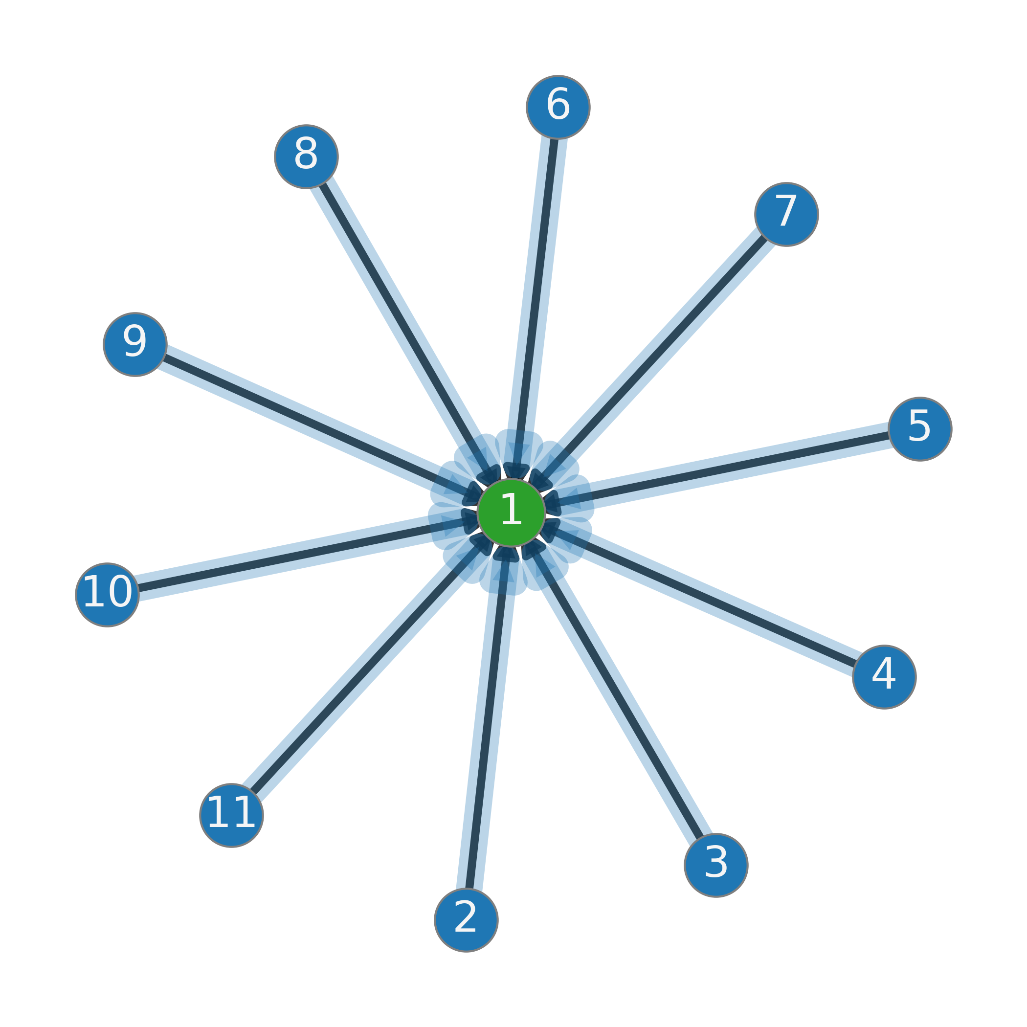
(a)

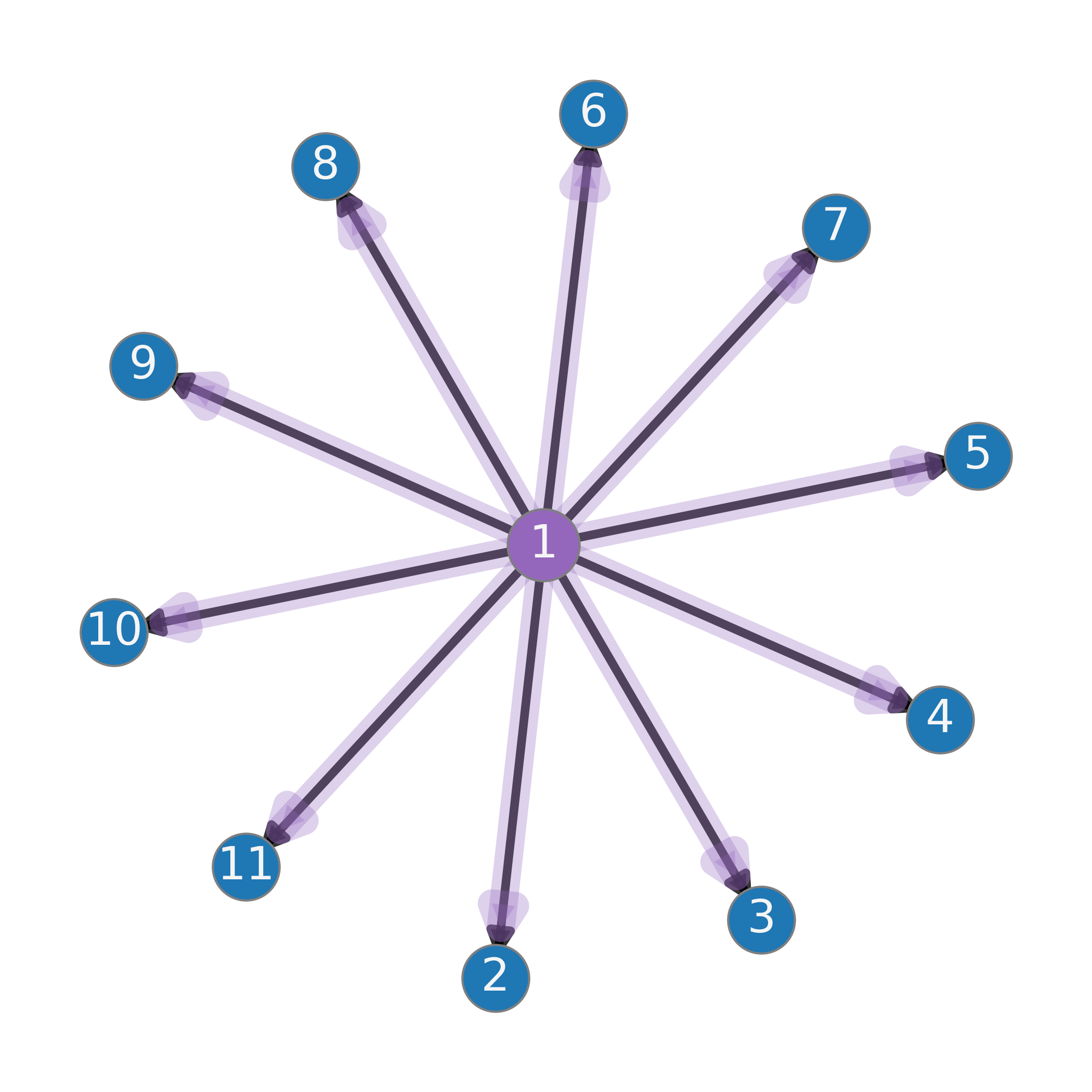
(b)

Figure 4: Directed stars (a) $G^{(\text{in})}$, and (b) $G^{(\text{out})}$

Example 1.

Let $G^{(\text{in})}$ and $G^{(\text{out})}$ be the directed star graphs with vertices $V=\{1,\ldots,N\}$ and edges pointing in/out to the central vertex as shown in Figure 4. Then the eigenvalues of $\mathbf{L}_{U}^{(q,\text{in})}$, the unnormalized magnetic Laplacian on $G^{\text{in}}$, are given by

$$\lambda_{1}^{\text{in}}=0,\quad\lambda_{k}^{\text{in}}=\frac{1}{2}\>\>\text{for }\>2\leq k\leq N-1,\quad\text{ and }\quad\lambda_{N}^{\text{in}}=\frac{N}{2}.$$

If we let $v=1$ be the central vertex, then the lead eigenvector is given by

$$\mathbf{u}^{\text{in}}_{1}(1)=e^{2\pi iq},\quad\mathbf{u}^{\text{in}}_{1}(n)=1,\>2\leq n\leq N.$$

For $2\leq k\leq N-1$, the eigenvectors are

$$\mathbf{u}^{\text{in}}_{k}=\bm{\delta}_{k}-\bm{\delta}_{k+1},$$

and the final eigenvector is given by

$$\mathbf{u}^{\text{in}}_{N}(1)=-e^{2\pi iq},\quad\mathbf{u}^{\text{in}}_{N}(n)=\frac{1}{N-1},\>2\leq n\leq N.$$

The phase matrices satisfies $\bm{\Theta}^{(q,\text{in})}=-\bm{\Theta}^{(q,\text{out})}$. Therefore, the associated magnetic Laplacians satisfy $\mathbf{L}_{U}^{(q,\text{in})}(u,v)=\overline{\mathbf{L}_{U}^{(q,\text{out})}(u,v)}.$ Since these matrices are Hermitian, this implies that the corresponding eigenvalue-eigenvector pairs satisfy $\lambda_{k}^{\text{in}}=\lambda_{k}^{\text{out}}$, and $\mathbf{u}_{k}^{\text{in}}=\overline{\mathbf{u}_{k}^{\text{out}}}$. Hence, $\mathbf{u}^{\text{in}}_{1}$ and $\mathbf{u}_{1}^{\text{out}}$ identify the central vertex, and the sign of their imaginary parts at this vertex identifies whether it is a source or a sink. On the other hand, the eigenvalues give no directional information.

Example 2.

Let $G$ be the directed cycle. Then, then the eigenvalues of $\mathbf{L}^{(q)}_{U}$ is are the classical Fourier modes $\mathbf{u}_{k}(n)=e^{(2\pi ikn/N)}$, independent of $q$. The eigenvalues, however, do depend on $q$ and are given by

$$\lambda_{k}=1-\cos\left(2\pi\left(\frac{k}{N}+q\right)\right),\quad 1\leq k\leq N.$$

Appendix G Expanded details of numerical results

Here we present more details on our node classification results in Tables 5, 6, 7, 8, and 9; and more details of our link prediction results in Tables 10, 11, 12, 13, 14, and 15. We present our results in the form mean $\pm$ standard deviation.

The networks GCN, APPNP, GAT, SAGE, and GIN were not designed with directed graphs as the primary motivation. Therefore, we implemented these methods in two ways: (i) with the original asymmetric adjacency matrix; and (ii) with a symmetrized adjacency matrix. For node classification, symmetrizing the adjacency matrix improved performance for most of these networks on most of the real datasets. We did not test the symmetric implementations on our synthetic DSBM datasets because these datasets, by design, place a heavy importance on directional information. For link prediction, on the other hand, we only use asymmetric adjacency matrices. In our tables below, GCN, APPNP, GAT, SAGE, and GIN refer to the implementations with the symmetrized adjacency matrix and GCN-D, APPNP-D, GAT-D, SAGE-D, and GIN-D refer to our implementation with the asymmetric matrix.

Tables 5, 6, 7, and 8 provide the precise node classification results for the four types of DSBM graphs introduced in Section 5.1.1 of the main text; they correspond to the plots in Figure 2 of the main text. Table 9 contains all of the information contained in Table 1 from the main text, but reports separately the results of GCN, APPNP, GAT, SAGE, and GIN (which use the symmetrized adjacency matrix) and the results of GCN-D, APPNP-D, GAT-D, SAGE-D, and GIN-D (which use the asymmetric adjacency matrix), whereas Table 1 in the main text reported only the best-performer between the two variants.

With respect to link prediction, there are many results here in the appendix in addition to what is reported in the main text. Table 10 is the same as Table 2 from the main text, except here in the appendix we also include the Texas data set. Table 11 expands upon Table 10 by considering the more difficult three-class classification problems described in Appendix D.2. All of the results in these tables include undirected edges and, if present, multi-edges, which have essentially random labels with respect to their directionality (see also Section D.2), and hence these results indicate the model’s ability to ignore these noisy labels. MagNet performs quite well across this slate of link prediction experiments (top performer in 15/20 experiments).

Tables 12, 13, 14, and 15 evaluate the same four link prediction tasks as Tables 10 and 11, except that undirected edges and multi-edges are not included in the training/validation/testing sets. Thus all labels are well-defined and noiseless. In this setting MagNet also performs very well, obtaining the top performance in 22/32 experiments across all four tables.

Aside from Table 14, MagNet achieves the highest testing accuracy in 20/24 experiments. Digraph achieves the highest testing accuracy in 3/8 experiments, and MagNet is best in 2/8 experiments as shown in Table 14. Having said that, there is not a statistically significant difference between MagNet and the top performing method in two other datasets (Wisconsin and Cora-ML), and MagNet is also a very close second on WikiCS. Thus, MagNet is either the top performer or on par with the top performing method in 5/8 datasets in Table 14. Nevertheless, the task is more difficult for MagNet than other tasks. We hypothesize that this is because half of the task is identifying whether there is an edge between $u,v$, or not; the other half, if there is an edge, is determining its direction. The first half of the task is an undirected task, and thus $q>0$ could provide noisy features for those pairs of vertices for which there is no edge. The Digraph method utilizes the symmetric Laplacian, which is unsuitable for direction prediction but works well for predicting the presence of an edge in either direction or the absence of an edge. The direction of the edge is more important in Tables 12, 13, and 15, and MagNet captures the direction information very well. The results indicate there is a trade-off between capturing undirected and directed features. This observation also leads to a potential future research direction that utilizes magnetic Laplacian matrices based on multiple values of $q$, making MagNet capture both undirected and directed information precisely.

Table 5: Node classification accuracy of ordered DSBM graphs with varying edge density.

Method / $\alpha^{\ast}$ 0.1 0.08 0.05 ChebNet 19.9$\pm$0.6 20.0$\pm$0.7 20.0$\pm$0.7 GCN-D 68.9$\pm$2.1 67.6$\pm$2.7 58.5$\pm$2.0 APPNP-D 97.7$\pm$1.7 95.9$\pm$2.2 90.3$\pm$2.4 SAGE-D 20.1$\pm$1.1 19.9$\pm$0.8 19.9$\pm$1.0 GIN-D 57.3$\pm$5.8 55.4$\pm$5.5 50.9$\pm$7.7 GAT-D 42.1$\pm$5.3 39.0$\pm$7.0 37.2$\pm$5.5 DGCN 84.9$\pm$7.2 81.2$\pm$8.2 64.4$\pm$12.4 DiGraph 82.1$\pm$1.7 77.7$\pm$1.6 66.1$\pm$2.4 DiGraphIB 99.2$\pm$0.5 97.7$\pm$0.7 89.3$\pm$1.7 MagNet 99.6$\pm$0.2 98.3$\pm$0.8 94.1$\pm$1.2 Best $q$ 0.25 0.10 0.25

Table 6: Node classification accuracy of ordered DSBM graphs with varying net flow.

Method / $\beta^{\ast}$ .05 .10 .15 .20 .25 .30 .35 .40 ChebNet 19.9$\pm$0.7 20.1$\pm$0.6 20.0$\pm$0.6 20.1$\pm$0.8 19.9$\pm$0.9 20.0$\pm$0.5 19.7$\pm$0.9 20.0$\pm$0.5 GCN-D 68.6$\pm$2.2 74.1$\pm$1.8 75.5$\pm$1.3 74.9$\pm$1.3 72.0$\pm$1.4 65.4$\pm$1.6 58.1$\pm$2.4 45.6$\pm$4.7 APPNP-D 97.4$\pm$1.8 94.3$\pm$2.4 89.4$\pm$3.6 79.8$\pm$9.0 69.4$\pm$3.9 59.6$\pm$4.9 51.8$\pm$4.5 39.4$\pm$5.3 SAGE-D 20.2$\pm$1.2 20.0$\pm$1.0 20.0$\pm$0.8 20.0$\pm$0.7 19.6$\pm$0.9 19.8$\pm$0.7 19.9$\pm$0.9 19.9$\pm$0.8 GIN-D 57.9$\pm$6.3 48.0$\pm$11.4 32.7$\pm$12.9 26.5$\pm$10.0 23.8$\pm$6.0 20.6$\pm$3.0 20.5$\pm$2.8 19.8$\pm$0.5 GAT-D 42.0$\pm$4.8 32.7$\pm$5.1 25.6$\pm$3.8 19.9$\pm$1.4 20.0$\pm$1.0 19.8$\pm$0.8 19.6$\pm$0.2 19.5$\pm$0.2 DGCN 81.4$\pm$1.1 84.7$\pm$0.7 85.5$\pm$1.0 86.2$\pm$0.8 84.2$\pm$1.1 78.4$\pm$1.3 69.6$\pm$1.5 54.3$\pm$1.5 DiGraph 82.5$\pm$1.4 82.9$\pm$1.9 81.9$\pm$1.1 79.7$\pm$1.3 73.5$\pm$1.9 67.4$\pm$2.8 57.8$\pm$1.6 43.0$\pm$7.1 DiGraphIB 99.2$\pm$0.4 97.9$\pm$0.6 94.1$\pm$1.7 88.7$\pm$2.0 82.3$\pm$2.7 70.0$\pm$2.2 57.8$\pm$6.4 41.0$\pm$9.0 MagNet 99.6$\pm$0.2 99.0$\pm$1.0 97.5$\pm$0.8 94.2$\pm$1.6 88.7$\pm$1.9 79.4$\pm$2.9 68.8$\pm$2.4 51.8$\pm$3.1 Best $q$ 0.25 0.20 0.20 0.25 0.20 0.20 0.20 0.25

Table 7: Node classification accuracy of cyclic DSBM graphs with varying net flow.

Method / $\beta^{\ast}$ .05 .10 .15 .20 .25 .30 ChebNet 74.7$\pm$16.5 65.4$\pm$22.2 70.5$\pm$22.7 64.6$\pm$31.6 85.0$\pm$8.7 60.1$\pm$19.8 GCN-D 78.8$\pm$30.0 81.2$\pm$14.7 69.5$\pm$4.2 58.6$\pm$37.2 75.4$\pm$7.4 43.6$\pm$32.4 APPNP-D 19.6$\pm$0.5 19.5$\pm$0.4 19.6$\pm$0.3 19.6$\pm$0.3 19.6$\pm$0.4 19.6$\pm$0.3 SAGE-D 88.6$\pm$8.3 81.9$\pm$17.2 81.4$\pm$8.4 73.5$\pm$20.6 79.2$\pm$10.5 59.7$\pm$25.3 GIN-D 75.3$\pm$21.5 66.9$\pm$24.7 53.9$\pm$15.4 68.7$\pm$19.8 62.3$\pm$20.3 41.6$\pm$18.2 GAT-D 98.3$\pm$2.2 80.6$\pm$30.7 95.5$\pm$12.4 59.7$\pm$39.2 93.1$\pm$4.4 68.7$\pm$35.9 DGCN 83.7$\pm$23.1 99.8$\pm$0.2 99.4$\pm$0.8 87.4$\pm$25.1 96.5$\pm$5.1 79.9$\pm$25.8 DiGraph 39.1$\pm$33.6 36.4$\pm$6.6 37.3$\pm$27.1 50.3$\pm$36.6 42.3$\pm$2.2 34.4$\pm$23.5 DiGraphIB 84.8$\pm$17.0 94.2$\pm$6.6 99.2$\pm$0.6 98.1$\pm$1.1 96.7$\pm$3.3 84.7$\pm$7.4 MagNet 100.0$\pm$0.0 99.9$\pm$0.2 87.4$\pm$28.4 96.8$\pm$12.5 100.0$\pm$0.0 99.4$\pm$0.6 Best $q$ 0.05 0.05 0.05 0.05 0.1 0.1

Table 8: Node classification accuracy of noisy cyclic DSBM graphs with varying net flow.

Method / $\beta^{\ast}$ .05 .10 .15 .20 ChebNet 18.3$\pm$3.1 18.8$\pm$3.8 18.9$\pm$3.3 19.3$\pm$3.4 GCN-D 24.2$\pm$6.8 22.8$\pm$4.1 21.3$\pm$3.5 20.3$\pm$4.4 APPNP-D 17.4$\pm$1.8 17.9$\pm$2.0 17.8$\pm$1.8 17.6$\pm$2.6 SAGE-D 26.4$\pm$7.7 21.7$\pm$5.5 20.1$\pm$4.5 20.0$\pm$3.8 GIN-D 24.7$\pm$6.4 20.2$\pm$3.8 22.2$\pm$4.6 20.0$\pm$3.8 GAT-D 27.4$\pm$6.9 24.6$\pm$5.1 21.9$\pm$4.6 21.6$\pm$4.2 DGCN 37.3$\pm$6.1 28.9$\pm$6.9 25.4$\pm$6.7 20.4$\pm$4.1 DiGraph 18.0$\pm$1.8 18.1$\pm$1.8 18.2$\pm$1.6 17.9$\pm$2.4 DiGraphIB 43.4$\pm$10.1 32.3$\pm$10.1 26.8$\pm$11.6 19.1$\pm$2.9 MagNet 80.5$\pm$7.0 63.7$\pm$8.2 56.9$\pm$6.7 70.2$\pm$5.1 Best $q$ 0.25 0.25 0.25 0.20

Table 9: Testing accuracy of node classification. The best results are in bold and the second best are underlined.

		Cornell	Texas	Wisconsin	Cora-ML	Citeseer	Telegram
ChebNet		79.8$\pm$5.0	79.2$\pm$7.5	81.6$\pm$6.3	80.0$\pm$1.8	66.7$\pm$1.6	73.4 $\pm$5.8
GCN		59.0$\pm$6.4	57.9$\pm$5.4	55.9$\pm$5.4	82.0$\pm$1.1	66.0$\pm$1.5	73.4$\pm$5.9
GCN-D		57.3$\pm$4.8	58.7$\pm$3.8	52.7$\pm$5.4	72.6$\pm$1.6	60.5$\pm$1.6	63.6$\pm$4.7
APPNP		58.7$\pm$4.0	57.0$\pm$4.8	49.6$\pm$6.5	82.6$\pm$1.4	66.9$\pm$1.8	69.4$\pm$3.5
APPNP-D		58.4$\pm$3.0	56.8$\pm$2.7	51.8$\pm$7.4	68.6$\pm$2.5	58.6$\pm$1.8	66.4$\pm$5.0
GAT		57.6$\pm$4.9	61.1$\pm$5.0	54.1$\pm$4.2	81.9$\pm$1.0	67.3$\pm$1.3	72.6$\pm$7.5
GAT-D		57.3$\pm$7.7	59.2$\pm$4.1	52.0$\pm$4.6	73.1$\pm$1.6	62.7$\pm$1.6	67.4$\pm$4.4
SAGE		77.6$\pm$6.3	84.3$\pm$5.5	79.2$\pm$5.3	82.3$\pm$1.2	66.0$\pm$1.5	56.6$\pm$6.0
SAGE-D		80.0$\pm$6.1	76.2$\pm$3.8	83.1$\pm$4.8	72.0$\pm$2.1	61.8$\pm$2.0	55.0$\pm$7.4
GIN		57.9$\pm$5.7	65.2$\pm$6.5	58.2$\pm$5.1	78.1$\pm$2.0	63.3$\pm$2.5	74.4$\pm$8.1
GIN-D		55.4$\pm$5.2	58.1$\pm$5.3	50.2$\pm$7.6	67.0$\pm$3.2	60.4$\pm$2.3	68.8$\pm$4.0
DGCN		67.3$\pm$4.3	71.7$\pm$7.4	65.5$\pm$4.7	81.3$\pm$1.4	66.3$\pm$2.0	90.4$\pm$5.6
Digraph		66.8$\pm$6.2	64.9$\pm$8.1	59.6$\pm$3.8	79.4$\pm$1.8	62.6$\pm$2.2	82.0$\pm$3.1
DiGraphIB		64.4$\pm$9.0	64.9$\pm$13.7	64.1$\pm$7.0	79.3$\pm$ 1.2	61.1$\pm$1.7	64.1$\pm$7.0
MagNet		84.3$\pm$7.0	83.3$\pm$6.1	85.7$\pm$3.2	79.8$\pm$2.5	67.5$\pm$1.8	87.6 $\pm$2.9
Best $q$		0.25	0.15	0.05	0.0	0.0	0.15

Table 10: Link prediction accuracy (%) with noisy labels. The best results are in bold and the second best are underlined.

Direction prediction Existence prediction Cornell Texas Wisconsin Cora-ML CiteSeer Cornell Texas Wisconsin Cora-ML CiteSeer ChebNet 71.0$\pm$5.5 66.8$\pm$6.9 67.5$\pm$4.5 72.7$\pm$1.5 68.0$\pm$1.6 80.1$\pm$2.3 81.7$\pm$2.7 82.5$\pm$1.9 80.0$\pm$0.6 77.4$\pm$0.4 GCN 56.2$\pm$8.7 69.8$\pm$4.9 71.0$\pm$4.0 79.8$\pm$1.1 68.9$\pm$2.8 75.1$\pm$1.4 76.1$\pm$3.0 75.1$\pm$1.9 81.6$\pm$0.5 76.9$\pm$0.5 APPNP 69.5$\pm$9.0 76.8$\pm$5.1 75.1$\pm$3.5 83.7$\pm$0.7 77.9$\pm$1.6 74.9$\pm$1.5 76.4$\pm$2.5 75.7$\pm$2.2 82.5$\pm$0.6 78.6$\pm$0.7 SAGE 75.2$\pm$11.0 69.8$\pm$5.9 72.0$\pm$3.5 68.2$\pm$0.8 68.7$\pm$1.5 79.8$\pm$2.4 75.2$\pm$3.1 77.3$\pm$2.9 75.0$\pm$0.0 74.1$\pm$1.0 GIN 69.3$\pm$6.0 76.1$\pm$4.5 74.8$\pm$3.7 83.2$\pm$0.9 76.3$\pm$1.4 74.5$\pm$2.1 77.5$\pm$3.8 76.2$\pm$1.9 82.5$\pm$0.7 77.9$\pm$0.7 GAT 67.9$\pm$11.1 50.0$\pm$2.0 53.2$\pm$2.6 50.0$\pm$0.1 50.6$\pm$0.5 77.9$\pm$3.2 74.9$\pm$0.3 74.6$\pm$0.0 75.0$\pm$0.0 75.0$\pm$0.0 DGCN 80.7$\pm$6.3 72.5$\pm$8.0 74.5$\pm$7.2 79.6$\pm$1.5 78.5$\pm$2.3 80.0$\pm$3.9 82.3$\pm$3.1 82.8$\pm$2.0 82.1$\pm$0.5 81.2$\pm$0.4 DiGraph 79.3$\pm$1.9 79.8$\pm$3.0 82.3$\pm$4.9 80.8$\pm$1.1 81.0$\pm$1.1 80.6$\pm$2.5 82.8$\pm$2.5 82.8$\pm$2.6 81.8$\pm$0.5 82.2$\pm$0.6 DiGraphIB 79.8$\pm$4.8 81.1$\pm$2.5 82.0$\pm$4.9 83.4$\pm$1.1 82.5$\pm$1.3 80.5$\pm$3.6 83.6$\pm$2.6 82.4$\pm$2.2 82.2$\pm$0.5 81.0$\pm$0.5 MagNet 80.7$\pm$2.7 79.5$\pm$3.7 83.6$\pm$2.8 86.1$\pm$0.9 85.1$\pm$0.8 80.6$\pm$3.8 83.8$\pm$3.3 82.9$\pm$2.6 82.8$\pm$0.7 79.9$\pm$0.5 Best $q$ 0.10 0.10 0.05 0.05 0.15 0.25 0.10 0.25 0.05 0.05

Table 11: Link prediction accuracy based on three classes labels(%) with noisy labels. The best results are in bold and the second best are underlined.

Three classes link prediction Direction prediction by three classes training Cornell Texas Wisconsin Cora-ML CiteSeer Cornell Texas Wisconsin Cora-ML CiteSeer ChebNet 60.0$\pm$2.3 64.8$\pm$2.4 65.9$\pm$2.8 64.8$\pm$0.7 58.0$\pm$0.9 70.7$\pm$2.8 58.9$\pm$4.7 67.0$\pm$4.1 72.6$\pm$1.3 67.8$\pm$1.8 GCN 51.9$\pm$3.2 54.1$\pm$3.0 51.7$\pm$2.6 66.9$\pm$0.5 54.6$\pm$1.2 56.0$\pm$8.1 69.8$\pm$5.4 68.0$\pm$3.2 79.7$\pm$1.1 68.8$\pm$2.2 APPNP 55.4$\pm$4.9 56.7$\pm$2.7 53.7$\pm$3.2 67.8$\pm$0.7 57.8$\pm$1.2 76.0$\pm$6.6 76.4$\pm$4.0 72.5$\pm$3.9 82.5$\pm$0.7 78.2$\pm$1.7 SAGE 62.1$\pm$4.2 52.2$\pm$2.6 56.4$\pm$3.9 50.0$\pm$0.0 48.9$\pm$1.1 74.8$\pm$6.7 69.5$\pm$4.2 71.4$\pm$3.6 68.2$\pm$0.9 68.7$\pm$1.8 GIN 52.3$\pm$5.2 57.6$\pm$2.4 54.9$\pm$3.5 68.0$\pm$0.8 56.8$\pm$1.3 69.5$\pm$5.5 76.6$\pm$4.3 74.2$\pm$4.0 83.2$\pm$1.0 76.3$\pm$1.3 GAT 57.3$\pm$6.4 50.0$\pm$0.0 49.9$\pm$0.8 50.0$\pm$0.0 50.0$\pm$0.1 69.0$\pm$6.8 50.5$\pm$1.7 51.4$\pm$2.4 50.1$\pm$0.1 50.2$\pm$0.6 DGCN 63.2$\pm$4.7 64.9$\pm$2.8 65.9$\pm$2.7 67.2$\pm$0.6 63.7$\pm$0.7 76.7$\pm$4.4 63.4$\pm$8.9 68.1$\pm$6.7 79.4$\pm$1.4 78.6$\pm$2.2 DiGraph 63.7$\pm$3.7 66.6$\pm$3.3 67.2$\pm$2.2 66.4$\pm$0.6 64.7$\pm$0.7 79.5$\pm$1.9 80.0$\pm$3.8 82.8$\pm$5.3 80.7$\pm$1.0 79.9$\pm$1.2 DiGraphIB 62.0$\pm$5.3 67.4$\pm$2.5 66.0$\pm$1.5 66.0$\pm$0.6 62.0$\pm$0.9 81.4$\pm$2.8 79.8$\pm$3.1 82.8$\pm$5.2 83.2$\pm$1.1 82.5$\pm$1.6 MagNet 64.5$\pm$4.3 67.6$\pm$3.5 66.5$\pm$2.4 67.7$\pm$0.9 60.4$\pm$0.9 83.3$\pm$3.5 80.5$\pm$5.5 85.7$\pm$2.6 86.2$\pm$0.8 84.8$\pm$1.3 Best $q$ 0.25 0.15 0.25 0.05 0.05 0.25 0.15 0.25 0.05 0.05

Table 12: Existence prediction(%) with noiseless labels. The best results are in bold and the second best are underlined.

Cornell Texas Wisconsin Cora-ML CiteSeer WikiCS Chameleon Squirrel ChebNet 68.6$\pm$5.1 67.7$\pm$9.9 70.1$\pm$5.6 71.2$\pm$0.8 66.0$\pm$1.6 78.4$\pm$0.3 88.7$\pm$0.3 90.4$\pm$0.2 GCN-D 56.7$\pm$10.4 66.1$\pm$7.5 62.9$\pm$6.0 75.5$\pm$1.1 64.0$\pm$1.8 78.3$\pm$0.3 90.1$\pm$0.3 92.0$\pm$0.2 APPNP-D 65.2$\pm$9.0 72.1$\pm$6.9 71.5$\pm$4.0 78.6$\pm$0.7 71.0$\pm$0.8 80.6$\pm$0.3 90.4$\pm$0.4 91.8$\pm$0.2 SAGE-D 71.2$\pm$7.7 66.6$\pm$7.2 70.5$\pm$5.5 70.1$\pm$1.4 64.0$\pm$1.6 62.2$\pm$0.3 86.1$\pm$0.6 83.7$\pm$0.2 GIN-D 63.8$\pm$7.1 72.1$\pm$5.7 70.1$\pm$3.6 78.3$\pm$1.0 70.1$\pm$0.9 80.5$\pm$0.3 90.4$\pm$0.4 92.1$\pm$0.1 GAT-D 62.6$\pm$9.9 50.0$\pm$1.8 50.9$\pm$1.6 50.0$\pm$0.1 50.2$\pm$0.5 50.2$\pm$0.3 50.1$\pm$0.2 58.8$\pm$13.4 DGCN 73.2$\pm$5.3 67.1$\pm$9.8 71.8$\pm$4.5 74.0$\pm$1.0 73.4$\pm$1.2 80.7$\pm$0.3 89.1$\pm$0.4 91.5$\pm$0.2 DiGraph 71.6$\pm$5.3 84.2$\pm$3.8 79.4$\pm$3.3 75.7$\pm$1.1 74.0$\pm$1.3 76.8$\pm$0.3 89.3$\pm$0.4 91.4$\pm$0.1 DiGraphIB 73.4$\pm$4.4 85.1$\pm$5.6 77.9$\pm$3.8 76.0$\pm$1.0 74.3$\pm$2.0 76.9$\pm$0.4 89.3$\pm$0.5 90.8$\pm$0.1 MagNet 74.7$\pm$5.4 85.6$\pm$4.5 80.1$\pm$6.2 77.9$\pm$1.0 76.9$\pm$1.4 83.3$\pm$0.2 90.7$\pm$0.4 91.5$\pm$0.2 Best $q$ 0.05 0.10 0.20 0.10 0.10 0.05 0.05 0.05

Table 13: Direction prediction(%) with noiseless labels. The best results are in bold and the second best are underlined.

Cornell Texas Wisconsin Cora-ML CiteSeer WikiCS Chameleon Squirrel ChebNet 74.1$\pm$5.6 72.3$\pm$10.0 69.9$\pm$6.2 73.3$\pm$1.2 69.2$\pm$2.1 71.1$\pm$0.3 94.6$\pm$0.2 95.3$\pm$0.2 GCN-D 54.4$\pm$8.8 76.7$\pm$6.3 73.8$\pm$4.2 80.8$\pm$1.1 70.8$\pm$2.3 78.4$\pm$0.2 97.2$\pm$0.2 97.2$\pm$0.1 APPNP-D 73.6$\pm$6.6 83.6$\pm$4.3 80.8$\pm$4.5 85.6$\pm$0.8 81.0$\pm$1.8 82.9$\pm$0.2 97.6$\pm$0.2 98.1$\pm$0.1 SAGE-D 77.0$\pm$5.5 77.7$\pm$6.5 76.4$\pm$3.8 69.3$\pm$0.5 70.1$\pm$1.6 56.0$\pm$0.2 94.4$\pm$0.3 93.6$\pm$1.8 GIN-D 69.4$\pm$6.6 84.7$\pm$4.5 80.6$\pm$3.8 84.5$\pm$0.9 78.5$\pm$1.4 82.9$\pm$0.1 97.6$\pm$0.2 98.0$\pm$0.1 GAT-D 71.8$\pm$10.1 51.1$\pm$1.8 52.2$\pm$2.0 50.1$\pm$0.2 50.7$\pm$0.5 50.2$\pm$0.4 50.5$\pm$1.3 68.6$\pm$16.8 DGCN 82.9$\pm$5.9 80.8$\pm$10.8 76.8$\pm$8.8 80.3$\pm$1.5 81.6$\pm$2.0 81.6$\pm$0.3 96.6$\pm$0.2 98.0$\pm$0.1 DiGraph 83.1$\pm$4.9 89.0$\pm$2.8 87.8$\pm$4.1 82.0$\pm$1.0 84.0$\pm$1.5 79.6$\pm$0.2 97.1$\pm$0.2 96.9$\pm$0.1 DiGraphIB 83.7$\pm$5.6 89.5$\pm$3.3 87.8$\pm$3.9 84.3$\pm$1.4 85.1$\pm$1.4 83.0$\pm$0.2 97.6$\pm$0.2 97.2$\pm$0.1 MagNet 88.8$\pm$4.9 91.9$\pm$4.5 89.3$\pm$4.2 87.3$\pm$0.8 88.1$\pm$0.9 86.2$\pm$0.2 97.8$\pm$0.2 98.1$\pm$0.1 Best $q$ 0.10 0.05 0.25 0.20 0.10 0.05 0.20 0.10

Table 14: Three classes link prediction(%) with noiseless labels. The best results are in bold and the second best are underlined.

Cornell Texas Wisconsin Cora-ML CiteSeer WikiCS Chameleon Squirrel ChebNet 63.0$\pm$2.1 71.5$\pm$2.0 70.5$\pm$2.1 65.6$\pm$0.5 60.3$\pm$0.8 74.3$\pm$0.1 80.7$\pm$0.3 83.9$\pm$0.1 GCN-D 53.0$\pm$2.5 62.6$\pm$2.6 55.8$\pm$3.1 67.5$\pm$0.6 57.1$\pm$1.1 74.5$\pm$0.2 81.3$\pm$0.3 86.2$\pm$0.1 APPNP-D 61.5$\pm$3.6 63.3$\pm$3.3 57.9$\pm$4.3 68.6$\pm$0.7 60.3$\pm$1.2 75.8$\pm$0.2 81.2$\pm$0.2 85.9$\pm$0.1 SAGE-D 64.8$\pm$4.0 59.2$\pm$3.2 60.7$\pm$4.6 50.9$\pm$0.1 51.1$\pm$1.2 60.8$\pm$0.1 70.0$\pm$0.3 67.3$\pm$0.2 GIN-D 54.6$\pm$3.8 65.2$\pm$3.7 58.4$\pm$4.0 68.6$\pm$0.7 59.1$\pm$1.4 76.2$\pm$0.2 81.7$\pm$0.3 86.5$\pm$0.3 GAT-D 58.8$\pm$6.4 56.9$\pm$1.4 54.2$\pm$1.0 50.8$\pm$0.1 52.2$\pm$0.2 60.8$\pm$0.1 54.2$\pm$0.1 52.5$\pm$0.0 DGCN 65.1$\pm$6.1 73.6$\pm$3.6 71.6$\pm$1.7 67.9$\pm$0.5 66.0$\pm$0.7 77.6$\pm$0.1 80.9$\pm$0.3 85.4$\pm$0.1 DiGraph 66.1$\pm$4.7 76.4$\pm$4.0 72.9$\pm$2.0 67.2$\pm$0.7 67.5$\pm$0.6 74.4$\pm$0.2 83.8$\pm$0.3 86.4$\pm$0.2 DiGraphIB 64.5$\pm$4.1 76.2$\pm$4.3 72.4$\pm$2.6 66.6$\pm$0.5 64.4$\pm$0.6 71.8$\pm$0.2 83.4$\pm$0.2 85.6$\pm$0.1 MagNet 66.4$\pm$5.0 76.6$\pm$3.9 71.3$\pm$2.3 68.4$\pm$0.8 63.2$\pm$1.3 77.0$\pm$0.2 81.9$\pm$0.4 84.8$\pm$0.1 Best $q$ 0.25 0.05 0.25 0.05 0.05 0.05 0.05 0.10

Table 15: Direction prediction by three classes link prediction(%) with noiseless labels. The best results are in bold and the second best are underlined.

Cornell Texas Wisconsin Cora-ML CiteSeer WikiCS Chameleon Squirrel Cheb 75.6$\pm$4.9 61.6$\pm$5.4 69.7$\pm$4.1 73.4$\pm$1.3 69.4$\pm$1.5 71.1$\pm$0.2 94.6$\pm$0.2 95.3$\pm$0.1 GCN-D 56.6$\pm$3.0 77.9$\pm$7.0 70.9$\pm$5.1 80.6$\pm$1.1 70.3$\pm$2.1 78.4$\pm$0.2 97.2$\pm$0.2 97.2$\pm$0.1 APPNP-D 75.5$\pm$4.5 83.5$\pm$4.4 79.9$\pm$3.4 83.6$\pm$0.8 80.7$\pm$1.4 82.7$\pm$0.2 97.5$\pm$0.2 98.0$\pm$0.1 SAGE-D 77.3$\pm$4.5 75.0$\pm$5.4 75.8$\pm$5.0 69.2$\pm$0.6 69.7$\pm$1.6 56.0$\pm$0.3 94.4$\pm$0.3 92.8$\pm$1.3 GIN-D 71.9$\pm$4.6 85.6$\pm$4.1 80.6$\pm$3.8 84.4$\pm$0.8 78.6$\pm$2.0 82.9$\pm$0.2 97.6$\pm$0.2 98.1$\pm$0.1 GAT-D 67.3$\pm$10.8 49.7$\pm$1.6 52.3$\pm$1.9 50.0$\pm$0.1 50.1$\pm$0.3 50.2$\pm$0.5 50.1$\pm$0.1 50.0$\pm$0.0 DGCN 79.9$\pm$6.1 68.0$\pm$8.9 77.0$\pm$4.3 80.1$\pm$1.1 81.1$\pm$2.6 81.6$\pm$0.3 96.4$\pm$0.2 98.0$\pm$0.1 DiGraph 85.5$\pm$4.1 90.4$\pm$4.0 87.6$\pm$4.7 82.0$\pm$1.0 83.0$\pm$1.2 79.6$\pm$0.2 97.1$\pm$0.2 96.9$\pm$0.1 DiGraphIB 85.2$\pm$4.7 89.9$\pm$3.4 87.5$\pm$4.2 84.2$\pm$1.1 85.2$\pm$1.3 82.2$\pm$0.3 97.1$\pm$0.2 96.9$\pm$0.1 MagNet 88.5$\pm$3.9 87.9$\pm$8.4 90.2$\pm$3.1 87.4$\pm$0.7 87.9$\pm$1.1 85.4$\pm$0.3 97.8$\pm$0.2 98.0$\pm$0.1 Best $q$ 0.25 0.05 0.25 0.05 0.05 0.05 0.05 0.10

Appendix H Optimal $q$ values for synthetic data

Optimal $q$ values for synthetic graphs are shown in Tables 5, 6, 7, and 8. We observe that the optimal $q$ is smaller for node classification of cyclic DSBM graphs than the ordered and noisy cyclic DSBM graphs. For cyclic DSBM graphs, the cluster is relatively clear by checking connectivity even without direction information. But the direction is crucial for classification for the other two types of DSBM graphs. It indicates that a smaller $q$ $(q<0.15)$ is enough for node classification of directed graphs when the direction is less critical. And a larger $q$ $(q>0.15)$ is needed to encode more direction information in the phase matrix for better performance. If the cluster is evident in the symmetrized adjacency matrix, we can use $q=0$, and MagNet will reduce to ChebNet as in the results on Cora-ML and CiteSeer in Table 9.

References

- [1] James Atwood and Don Towsley. Diffusion-convolutional neural networks. In D. Lee, M. Sugiyama, U. Luxburg, I. Guyon, and R. Garnett, editors, Advances in Neural Information Processing Systems, volume 29, pages 1993–2001. Curran Associates, Inc., 2016.
- [2] Mikhail Belkin and Partha Niyogi. Laplacian eigenmaps for dimensionality reduction and data representation. Neural computation, 15(6):1373–1396, 2003.
- [3] Austin R Benson, David F Gleich, and Jure Leskovec. Higher-order organization of complex networks. Science, 353(6295):163–166, 2016.
- [4] Aleksandar Bojchevski and Stephan Günnemann. Deep gaussian embedding of graphs: Unsupervised inductive learning via ranking. In ICLR Workshop on Representation Learning on Graphs and Manifolds, 2017.
- [5] Alexandre Bovet and Peter Grindrod. The activity of the far right on telegram. https://www.researchgate.net/publication/346968575_The_Activity_of_the_Far_Right_on_Telegram_v21, 2020.
- [6] Joan Bruna, Wojciech Zaremba, Arthur Szlam, and Yann LeCun. Spectral networks and deep locally connected networks on graphs. In International Conference on Learning Representations (ICLR), 2014.
- [7] Fan Chung. Laplacians and the cheeger inequality for directed graphs. Annals of Combinatorics, 9(1):1–19, 2005.
- [8] Fan Chung and Mark Kempton. A local clustering algorithm for connection graphs. In International Workshop on Algorithms and Models for the Web-Graph, pages 26–43. Springer, 2013.
- [9] Fan RK Chung and Fan Chung Graham. Spectral graph theory. Number 92. American Mathematical Soc., 1997.
- [10] Alexander Cloninger. A note on markov normalized magnetic eigenmaps. Applied and Computational Harmonic Analysis, 43(2):370 – 380, 2017.
- [11] Ronald R Coifman and Stéphane Lafon. Diffusion maps. Applied and computational harmonic analysis, 21(1):5–30, 2006.
- [12] Mihai Cucuringu, Huan Li, He Sun, and Luca Zanetti. Hermitian matrices for clustering directed graphs: insights and applications. In International Conference on Artificial Intelligence and Statistics, pages 983–992. PMLR, 2020.
- [13] Michaël Defferrard, Xavier Bresson, and Pierre Vandergheynst. Convolutional neural networks on graphs with fast localized spectral filtering. In Advances in Neural Information Processing Systems 29, pages 3844–3852, 2016.
- [14] David K Duvenaud, Dougal Maclaurin, Jorge Iparraguirre, Rafael Bombarell, Timothy Hirzel, Alan Aspuru-Guzik, and Ryan P Adams. Convolutional networks on graphs for learning molecular fingerprints. In C. Cortes, N. Lawrence, D. Lee, M. Sugiyama, and R. Garnett, editors, Advances in Neural Information Processing Systems, volume 28, pages 2224–2232. Curran Associates, Inc., 2015.
- [15] Bruno Messias F. de Resende and Luciano da F. Costa. Characterization and comparison of large directed networks through the spectra of the magnetic laplacian. Chaos: An Interdisciplinary Journal of Nonlinear Science, 30(7):073141, 2020.
- [16] Michaël Fanuel, Carlos M. Alaíz, Ángela Fernández, and Johan A.K. Suykens. Magnetic eigenmaps for the visualization of directed networks. Applied and Computational Harmonic Analysis, 44:189–199, 2018.
- [17] Michaël Fanuel, Carlos M Alaiz, and Johan AK Suykens. Magnetic eigenmaps for community detection in directed networks. Physical Review E, 95(2):022302, 2017.
- [18] Satoshi Furutani, Toshiki Shibahara, Mitsuaki Akiyama, Kunio Hato, and Masaki Aida. Graph signal processing for directed graphs based on the hermitian laplacian. In Machine Learning and Knowledge Discovery in Databases, pages 447–463, 2020.
- [19] Krystal Guo and Bojan Mohar. Hermitian adjacency matrix of digraphs and mixed graphs. Journal of Graph Theory, 85(1):217–248, 2017.
- [20] William L. Hamilton, Rex Ying, and Jure Leskovec. Inductive representation learning on large graphs. In Proceedings of the 31st International Conference on Neural Information Processing Systems, NIPS’17, page 1025–1035, Red Hook, NY, USA, 2017. Curran Associates Inc.
- [21] David K Hammond, Pierre Vandergheynst, and Rémi Gribonval. Wavelets on graphs via spectral graph theory. Applied and Computational Harmonic Analysis, 30(2):129–150, 2011.
- [22] Thomas N. Kipf and Max Welling. Semi-supervised classification with graph convolutional networks. In International Conference on Learning Representations (ICLR), 2017.
- [23] Johannes Klicpera, Aleksandar Bojchevski, and Stephan Günnemann. Predict then propagate: Graph neural networks meet personalized pagerank. In ICLR, 2019.
- [24] Ron Levie, Wei Huang, Lorenzo Bucci, Michael M Bronstein, and Gitta Kutyniok. Transferability of spectral graph convolutional neural networks. arXiv preprint arXiv:1907.12972, 2019.
- [25] Elliott H Lieb and Michael Loss. Fluxes, laplacians, and kasteleyn’s theorem. In Statistical Mechanics, pages 457–483. Springer, 1993.
- [26] Yi Ma, Jianye Hao, Yaodong Yang, Han Li, Junqi Jin, and Guangyong Chen. Spectral-based graph convolutional network for directed graphs. arXiv:1907.08990, 2019.
- [27] Antonio G Marques, Santiago Segarra, and Gonzalo Mateos. Signal processing on directed graphs: The role of edge directionality when processing and learning from network data. IEEE Signal Processing Magazine, 37(6):99–116, 2020.
- [28] Péter Mernyei and Cătălina Cangea. Wiki-cs: A wikipedia-based benchmark for graph neural networks. arXiv preprint arXiv:2007.02901, 2020.
- [29] Bojan Mohar. A new kind of hermitian matrices for digraphs. Linear Algebra and its Applications, 584:343–352, 2020.
- [30] Federico Monti, Karl Otness, and Michael M. Bronstein. Motifnet: A motif-based graph convolutional network for directed graphs. In 2018 IEEE Data Science Workshop, pages 225–228, 2018.
- [31] Antonio Ortega, Pascal Frossard, Jelena Kovačević, José MF Moura, and Pierre Vandergheynst. Graph signal processing: Overview, challenges, and applications. Proceedings of the IEEE, 106(5):808–828, 2018.
- [32] Hongbin Pei, Bingzhe Wei, Kevin Chen-Chuan Chang, Yu Lei, and Bo Yang. Geom-gcn: Geometric graph convolutional networks. arXiv preprint arXiv:2002.05287, 2020.
- [33] Benedek Rozemberczki, Carl Allen, and Rik Sarkar. Multi-scale attributed node embedding. arXiv preprint arXiv:1909.13021, 2019.
- [34] Jianbo Shi and Jitendra Malik. Normalized cuts and image segmentation. In Proceedings of IEEE computer society conference on computer vision and pattern recognition, pages 731–737. IEEE, 1997.
- [35] Daniel A Spielman and Shang-Hua Teng. Nearly-linear time algorithms for graph partitioning, graph sparsification, and solving linear systems. In Proceedings of the thirty-sixth annual ACM symposium on Theory of computing, pages 81–90, 2004.
- [36] Z. Tong, Yuxuan Liang, Changsheng Sun, Xinke Li, David S. Rosenblum, and A. Lim. Digraph inception convolutional networks. In NeurIPS, 2020.
- [37] Zekun Tong, Yuxuan Liang, Changsheng Sun, David S. Rosenblum, and Andrew Lim. Directed graph convolutional network. arXiv:2004.13970, 2020.
- [38] Petar Veličković, Guillem Cucurull, Arantxa Casanova, Adriana Romero, Pietro Liò, and Yoshua Bengio. Graph Attention Networks. International Conference on Learning Representations, 2018.
- [39] Palmer W.R. and Zheng T. Spectral clustering for directed networks. Studies in Computational Intelligence, 943, 2021.
- [40] Zonghan Wu, Shirui Pan, Fengwen Chen, Guodong Long, Chengqi Zhang, and Philip S. Yu. A comprehensive survey on graph neural networks. IEEE Transactions on Neural Networks and Learning Systems, 32(1):4–24, 2020.
- [41] Keyulu Xu, Weihua Hu, Jure Leskovec, and Stefanie Jegelka. How powerful are graph neural networks? arXiv preprint arXiv:1810.00826, 2018.
- [42] Jie Zhou, Ganqu Cui, Zhengyan Zhang, Cheng Yang, Zhiyuan Liu, Lifeng Wang, Changcheng Li, and Maosong Sun. Graph neural networks: A review of methods and applications. arXiv preprint arXiv:1812.08434, 2018.