A new Wilson line-based action for gluodynamics

Abstract

We perform a canonical transformation of fields that brings the Yang-Mills action in the light-cone gauge to a new classical action, which does not involve any triple-gluon vertices. The lowest order vertex is the four-point MHV vertex. Higher point vertices include the MHV and $\overline{\textrm{MHV}}$ vertices, that reduce to the corresponding amplitudes in the on-shell limit. In general, any $n$-leg vertex has $2\leq m\leq n-2$ negative helicity legs. The canonical transformation of fields can be compactly expressed in terms of path-ordered exponentials of fields and their functional derivative. We apply the new action to compute several tree-level amplitudes, up to 8-point NNMHV amplitude, and find agreement with the standard methods. The absence of triple-gluon vertices results in fewer diagrams required to compute amplitudes, when compared to the CSW method and, obviously, considerably fewer than in the standard Yang-Mills action.

1 Introduction

Although quark and gluon fields are considered to be the most fundamental degrees of freedom of Quantum Chromodynamics (QCD), in a variety of situations they are definitely not the most effective ones. There are several quite distinct aspects of the QCD theory where this becomes manifest. For example, in QCD factorization theorems, which are essential tools to relate the theory to high energy experiments, one needs to account not just for a single quark or gluon exchanged between subprocesses separated by a large energy scale, but also for all collinear and soft gluons; these resummed exchanges of gluons can be included by using Wilson lines (see [1] for a comprehensive review of the factorization theorems). Similar collective degrees of freedom appear naturally in the high energy limit of QCD (see e.g. [2, 3]). In the domain of non-perturbative QCD, further example can be provided by lattice QCD, where instead of the gauge fields one uses Wilson lines and Wilson loops. It is also known that, in the limit of large number of colors, the gauge theory can be completely formulated in loop space, i.e. in terms of various contours of the Wilson loop [4] (see also a textbook [5]).

The subject of interest of the following work are scattering amplitudes, in particular the pure gluonic amplitudes. In that context, it is already well understood that the elementary triple and four-gluon interactions are not the most effective bricks to build the amplitudes. Pictorially, they are way too small, so that the number of Feynman diagrams can become intractable for multi gluon processes. Instead, one should rather use the smaller amplitudes (i.e. with fewer legs) as the building blocks, but they must be deformed to the non-physical domain according to the Britto-Cachazo-Feng-Witten (BCFW) method [6, 7]. A particularly interesting example of the BCFW method is when the only type of amplitudes used are the maximally helicity violating (MHV) amplitudes [8]. This type of recursion has been found earlier based on the twistor space formulation of quantum field theory by Cachazo, Svrcek and Witten (CSW) [9], who suggested that the MHV amplitudes continued off-shell are really the multileg vertices (this formalism was later proved to be equivalent to the standard Yang-Mills theory in [10]). Indeed, an explicit action has been found, where the MHV vertices are reproduced as a result of the canonical field transformation on the Yang-Mills action in light-cone gauge [11, 12] This so-called ”MHV action” has also been developed for spontaneously broken gauge theory in [13] and also for supersymmetric gauge theories in [14, 15, 16]. It was also shown that the action reproduces correctly the one-loop same helicity amplitudes [17, 18, 19, 20, 21, 22, 23]. Furthermore, in the supersymmetric regime, using the MHV vertices, MHV loop amplitudes in $\mathcal{N}=4$ super Yang-Mills theory were derived explicitly in [24]. This was later extended for $\mathcal{N}=1$ (and $\mathcal{N}=2$) super Yang-Mills in [25]. Following this, non-supersymmetric one-loop amplitudes, using MHV diagrams, were explored in [26].

Interestingly, the new fields appearing in the MHV action turn out to be related to the straight infinite Wilson line of the Yang-Mills fields [27, 28].

As the above result is central to the present paper, let us describe it in more detail. The light-cone Yang-Mills action can be expressed in terms of just two transverse gluon fields, that correspond to two polarization states in the on-shell limit. The MHV action is obtained by transforming both fields to a new pair of fields. In [27] it was found that the plus helicity field in the MHV action is given as the straight infinite Wilson line along the complex direction determined by the plus helicity polarization vector. This means that the line lies on the so-called self-dual plane, i.e. the plane on which the tensors are self-dual. In the recent paper [28], we found that the minus helicity field is given by a similar Wilson line, but with an insertion of the minus helicty gluon field somewhere on the line. Additionally, we postulated, that it should be a part of a bigger structure, extending beyond the self-dual plane.

Indeed, in the present work we find a more general canonical transformation based on path ordered exponentials of the gauge fields, extending over both the self-dual and anti-self-dual planes. The field transformation can be most easily derived as a subsequent canonical transformation of the anti-self-dual part of the MHV action, but we also discuss a direct link between the new action and the Yang-Mills action. The key property of the new action is that it does not have the triple-gluon vertices at all. The reason for this structure is that the triple-gluon vertices have been effectively resummed inside the Wilson lines. The absence of the $(++-)$ vertex already occurs at the level of the MHV action, as previously demonstrated in [11]. The second canonical transformation of the anti-self-dual part of the MHV action results in the absence of $(--+)$ triple-gluon vertex as well. Thus, the lowest multiplicity vertex is the four-point MHV vertex. Higher-point vertices include not only the MHV vertices, but also other helicity configurations. The number of diagrams needed to obtain amplitudes beyond the MHV level is thus greatly reduced. We perform explicit calculations within the new formulation of several higher multiplicity amplitudes, to verify the consistency of the results.

The paper is organized as follows. In Section 2 we introduce the new action, first on a general ground, and then we proceed to a more technical derivation. In Section 3 we apply the new theory to actual amplitude computations. In Section 4 we summarize the work and discuss some aspects of the new action, in particular the geometric picture behind the field transformation. Finally, in the Appendix we provide more technical details of selected calculations.

2 A new classical action for gluodynamics

2.1 General idea

Motivated by our earlier results [27, 28], we look for a new set of classical fields describing scattering processes with gluons in the simplest possible way. That is, we want to find an action, which has interaction vertices as close to the real scattering processes, as possible. It is known, that the lowest non-zero scattering amplitude in the physical domain (i.e. on-shell real momenta satisfying the momentum conservation) is the four-point amplitude. Therefore, we will look for an action that has no triple-field coupling. In addition, we want the new fields to have a closed form in terms of the ordinary Yang-Mills fields. This is necessary for practical applications of the new action.

In general, a field transformation relates four components of fields, thus, in principle we have four transformations. In order to reduce the number of degrees of freedom, our starting point will be the Yang-Mills Lagrangian in the light-cone gauge, on the constant light-cone time $x^{+}$. As we shall recall below, such formulation reduces the four components of the gauge field $\hat{A}^{\mu}=t^{a}A_{a}^{\mu}$ to just two. Here, $t^{a}$ are color generators in the fundamental representation. To this end, we introduce the ”plus” and ”minus” light-cone coordinates for a four-vector $v^{\mu}$

$$v^{+}=v\cdot\eta\,,\,\,\,\,v^{-}=v\cdot\widetilde{\eta}\,,$$ (1)

where $\eta=\left(1,0,0,-1\right)/\sqrt{2}$, $\widetilde{\eta}=\left(1,0,0,1\right)/\sqrt{2}$, and two transverse coordinates

$$v^{\bullet}=v\cdot\varepsilon_{\bot}^{+}\,,\,\,\,\,v^{\star}=v\cdot\varepsilon_{\bot}^{-}\,,$$ (2)

defined by the complex null vectors $\varepsilon_{\perp}^{\pm}=\left(0,1,\pm i,0\right)/\sqrt{2}$. The scalar product of two four-vectors in these coordinates reads $u\cdot w=u^{+}w^{-}+u^{-}w^{+}-u^{\bullet}w^{\star}-u^{\star}w^{\bullet}$. In order to lower the indices one needs to flip $+\leftrightarrow-$ and $\star\leftrightarrow\bullet$, where the latter operation also causes a sign change.

The light-cone Yang-Mills action is obtained by setting the light-cone gauge $\hat{A}^{+}=0$ and integrating out the $\hat{A}^{-}$ field from the partition function. The resulting action has only two transverse fields $\hat{A}^{\bullet}$ and $\hat{A}^{\star}$ and reads [29]

$$S_{\mathrm{Y-M}}^{\left(\mathrm{LC}\right)}\left[A^{\bullet},A^{\star}\right]=\int dx^{+}\int d^{3}\mathbf{x}\,\,\Bigg{\{}-\mathrm{Tr}\,\hat{A}^{\bullet}\square\hat{A}^{\star}-2ig\,\mathrm{Tr}\,\partial_{-}^{-1}\partial_{\bullet}\hat{A}^{\bullet}\left[\partial_{-}\hat{A}^{\star},\hat{A}^{\bullet}\right]\\ -2ig\,\mathrm{Tr}\,\partial_{-}^{-1}\partial_{\star}\hat{A}^{\star}\left[\partial_{-}\hat{A}^{\bullet},\hat{A}^{\star}\right]-2g^{2}\,\mathrm{Tr}\,\left[\partial_{-}\hat{A}^{\bullet},\hat{A}^{\star}\right]\partial_{-}^{-2}\left[\partial_{-}\hat{A}^{\star},\hat{A}^{\bullet}\right]\Bigg{\}}\,,$$ (3)

where the bold position-space three-vector is defined as $\mathbf{x}\equiv\left(x^{-},x^{\bullet},x^{\star}\right)$ so that $x=(x^{+},\mathbf{x})$. The nabla operator reads $\square=2(\partial_{+}\partial_{-}-\partial_{\bullet}\partial_{\star})$ in these coordinates. The presence of just the physical degrees of freedom in the action leads to a natural identification of the helicity content of the vertices. Assigning the ”plus” helicity to $\hat{A}^{\bullet}$ field , and the ”minus” helicity to the field $\hat{A}^{\star}$, we see that there are $(++-)$, $(--+)$ and $(++--)$ vertices in the action.

Following the idea of [11], we look for a field transformation

$$\left\{\hat{A}^{\bullet},\hat{A}^{\star}\right\}\rightarrow\Big{\{}\hat{Z}^{\bullet}\big{[}{A}^{\bullet},{A}^{\star}\big{]},\hat{Z}^{\star}\big{[}{A}^{\bullet},{A}^{\star}\big{]}\Big{\}}\,,$$ (4)

which maps the kinetic term and both the triple-gluon vertices into a free term in the new action. In addition, we demand that the transformation is canonical, so that the functional measure in the partition function is preserved, up to a field independent factor.

Before we present the details on the transformation facilitating the above requirements, let us make some introductory remarks. Suppose we have a set of generalized coordinates and momenta $q_{i}$, $p_{i}$. Consider a canonical transformation to a new set $Q_{i}$, $P_{i}$. Consider now a particular generating function $\mathcal{G}$ for the canonical transformation between $\{q,p\}$ and $\{Q,P\}$, depending only on the generalized coordinates, $\mathcal{G}(q,Q)$. Then, the relation between the original and the transformed coordinates is

$$p_{i}=\frac{\partial\mathcal{G}(q,Q)}{\partial q_{i}}\,,\qquad P_{i}=-\frac{\partial\mathcal{G}(q,Q)}{\partial Q_{i}}\,.$$ (5)

In our context, the role of $q_{i}$ coordinate is played by the $\hat{A}^{\bullet}(x)$ field, and the canonical momentum $p_{i}$ is $\partial_{-}\hat{A}^{\star}(x)$. In the new theory, we identify $Q_{i}$ with $\hat{Z}^{\star}(x)$ and $P_{i}$ with $\partial_{-}\hat{Z}^{\bullet}(x)$. Therefore, the analogous relations are

$$\partial_{-}A^{\star}_{a}(x^{+},\mathbf{y})=\frac{\delta\,\mathcal{G}[A^{\bullet},Z^{\star}](x^{+})}{\delta A_{a}^{\bullet}\left(x^{+},\mathbf{y}\right)}\,,\qquad\partial_{-}Z^{\bullet}_{a}(x^{+},\mathbf{y})=-\frac{\delta\,\mathcal{G}[A^{\bullet},Z^{\star}](x^{+})}{\delta Z_{a}^{\star}\left(x^{+},\mathbf{y}\right)}\,,$$ (6)

where we have explicitly denoted the fact, that the transformation is performed on the hyper-surface of constant light-cone time $x^{+}$. Although the transformation (4) is rather complicated, we found that, quite amazingly, the generating functional $\mathcal{G}[A^{\bullet},Z^{\star}]$ can be written in the following simple form:

$$\mathcal{G}[A^{\bullet},Z^{\star}](x^{+})=-\int\!d^{3}\mathbf{x}\,\,\,\mathrm{Tr}\,\hat{\mathcal{W}}^{\,-1}_{(-)}[Z](x)\,\,\partial_{-}\hat{\mathcal{W}}_{(+)}[A](x)\,,$$ (7)

where the functional $\mathcal{W}_{(\pm)}[K]$, for a generic vector field $K^{\mu}$, is directly related to the straight infinite Wilson line in the following way:

$$\mathcal{W}^{a}_{(\pm)}[K](x)=\int_{-\infty}^{\infty}d\alpha\,\mathrm{Tr}\left\{\frac{1}{2\pi g}t^{a}\partial_{-}\,\mathbb{P}\exp\left[ig\int_{-\infty}^{\infty}\!ds\,\varepsilon_{\alpha}^{\pm}\cdot\hat{K}\left(x+s\varepsilon_{\alpha}^{\pm}\right)\right]\right\}\,,$$ (8)

with

$$\varepsilon_{\alpha}^{\pm\,\mu}=\varepsilon_{\perp}^{\pm\,\mu}-\alpha\eta^{\mu}\,.$$ (9)

The above four vector has the form of a gluon polarization vector. Indeed for $\alpha=p\cdot\varepsilon_{\perp}^{\pm}/p^{+}$, it is the transverse polarization vector for a gluon with momentum $p$. This type of functional has been used for the first time in [27] in the context of the MHV Lagrangian. The inverse functional to the Wilson line, $\mathcal{W}^{-1}$, is defined using the relation $\mathcal{W}[\mathcal{W}^{-1}[K]]=K$. Note, that the functionals $\mathcal{W}_{(+)}$ and $\mathcal{W}_{(-)}$ are not exactly hermitian conjugates of each other; only the projection on $\varepsilon_{\alpha}^{+}$ or $\varepsilon_{\alpha}^{-}$ changes inside the path-ordered exponential, but the sign of $ig$ remains unchanged.

In the following sections we shall present more details on the implication of the transformation given by (6) and the exact form of the vertices in the new action. In the remaining part of this section, we will outline the general structure of the new action.

From Eqs. (6)-(7) one can see that the fields $\hat{A}^{\bullet}$ and $\hat{A}^{\star}$ have the following general expansion in terms of the new fields:

$$A_{a}^{\bullet}(x^{+};\mathbf{x})=\sum_{n=1}^{\infty}\int\!d^{3}\mathbf{y}_{1}\dots d^{3}\mathbf{y}_{n}\sum_{i=1}^{n}\,\Xi_{i,n-i}^{ab_{1}\dots b_{n}}(\mathbf{x};\mathbf{y}_{1},\dots,\mathbf{y}_{n})\prod_{k=1}^{i}Z_{b_{k}}^{\bullet}(x^{+};\mathbf{y}_{k})\prod_{l=i+1}^{n}Z_{b_{l}}^{\star}(x^{+};\mathbf{y}_{l})\,,$$ (10)

$$A_{a}^{\star}(x^{+};\mathbf{x})=\sum_{n=1}^{\infty}\int\!d^{3}\mathbf{y}_{1}\dots d^{3}\mathbf{y}_{n}\sum_{i=1}^{n}\,\Lambda_{i,n-i}^{ab_{1}\dots b_{n}}(\mathbf{x};\mathbf{y}_{1},\dots,\mathbf{y}_{n})\prod_{k=1}^{i}Z_{b_{k}}^{\star}(x^{+};\mathbf{y}_{k})\prod_{l=i+1}^{n}Z_{b_{l}}^{\bullet}(x^{+};\mathbf{y}_{l})\,,$$ (11)

where $\Xi_{i,j}^{ab_{1}\dots b_{i+j}}(\mathbf{x};\mathbf{y}_{1}\dots\mathbf{y}_{i+j})$ is an apriori unknown kernel for $i$ number of $Z^{\bullet}$ fields and $j$ number of $Z^{\star}$ fields in the expansion of $\hat{A}^{\bullet}$, depending on the adjoint color indices $a,b_{1}\dots b_{i+j}$ and not depending on the light-cone time. Similarly, $\Lambda_{i,j}^{ab_{1}\dots b_{i+j}}(\mathbf{x};\mathbf{y}_{1}\dots\mathbf{y}_{i+j})$ is the kernel for $i$ number of $Z^{\star}$ fields and $j$ number of $Z^{\bullet}$ fields in the expansion of $\hat{A}^{\star}$. At lowest order we must have

$$A_{a}^{\bullet}(x^{+};\mathbf{x})=Z_{a}^{\bullet}(x^{+};\mathbf{x})+\dots\,\,,\qquad A_{a}^{\star}(x^{+};\mathbf{x})=Z_{a}^{\star}(x^{+};\mathbf{x})+\dots\,\,.$$ (12)

In principle, one could find explicitly the kernels $\Xi_{i,j}$, $\Lambda_{i,j}$ from Eqs. (6)-(7). However, as we demonstrate in the next section, there is a much better way of doing that, which utilizes the existing results on the MHV Lagrangian [27, 28]. Since we want to describe a general structure of the action, for the rest of this section we shall assume that the kernels are known.

Inserting the solutions (10)-(11) to the Yang-Mills action (3), we find the following structure of the new action:

$$S_{\mathrm{Y-M}}^{\left(\mathrm{LC}\right)}\left[Z^{\bullet},Z^{\star}\right]=\int dx^{+}\Bigg{\{} -\int d^{3}\mathbf{x}\,\mathrm{Tr}\,\hat{Z}^{\bullet}\square\hat{Z}^{\star}$$

$$+\mathcal{L}^{(\mathrm{LC})}_{--++}+\mathcal{L}^{(\mathrm{LC})}_{--+++}+\mathcal{L}^{(\mathrm{LC})}_{--++++}+\dots$$

$$+\mathcal{L}^{(\mathrm{LC})}_{---++}+\mathcal{L}^{(\mathrm{LC})}_{---+++}+\mathcal{L}^{(\mathrm{LC})}_{---++++}+\dots$$

$$\,\,\vdots$$

$$+\mathcal{L}^{(\mathrm{LC})}_{---\dots-++}+\mathcal{L}^{(\mathrm{LC})}_{---\dots-+++}+\mathcal{L}^{(\mathrm{LC})}_{---\dots-++++}+\dots\Bigg{\}}\,,$$ (13)

where the $n$-point interaction vertex, $n\geq 4$, that couples $m$ minus helicity fields, $m\geq 2$, and $n-m$ plus helicity fields, has the following general form:

$$\mathcal{L}_{\underbrace{-\,\cdots\,-}_{m}\underbrace{+\,\cdots\,+}_{n-m}}^{\left(\mathrm{LC}\right)}=\int\!d^{3}\mathbf{y}_{1}\dots d^{3}\mathbf{y}_{n}\,\,\mathcal{U}^{b_{1}\dots b_{n}}_{-\dots-+\dots+}\left(\mathbf{y}_{1},\cdots\mathbf{y}_{n}\right)\prod_{i=1}^{m}Z^{\star}_{b_{i}}(x^{+};\mathbf{y}_{i})\prod_{j=1}^{n-m}Z^{\bullet}_{b_{j}}(x^{+};\mathbf{y}_{j})\,.$$ (14)

The above action has the following properties, which we will elaborate on in the next sections:

1. There are no three point interaction vertices.

2. At the classical level there are no all-plus, all-minus, as well as $(-+\dots+)$, $(-\dots-+)$ vertices.

3. There are MHV vertices, $(--+\dots+)$, corresponding to MHV amplitudes in the on-shell limit.

4. There are $\overline{\mathrm{MHV}}$ vertices, $(-\dots-++)$, corresponding to $\overline{\mathrm{MHV}}$ amplitudes in the on-shell limit.

5. All vertices have the form which can be easily calculated.

Because the lowest vertex is the single MHV four-point vertex that corresponds to the four-gluon MHV amplitude in the on-shell limit, the new action provides an efficient way to construct tree amplitudes with high multiplicity of legs, as we will demonstrate later in Section 3 by computing several examples.

2.2 Derivation

As we shall see in the following, the easiest way to derive the action (13) from the Yang-Mills action (3) is to first transform the latter into an action containing the MHV vertices. Thus, we start by a brief summary of this procedure.

2.2.1 MHV action

As explained in detail in [11], the MHV action implementing the CSW rules [9] is obtained by performing a canonical field transformation with a requirement that the kinetic term and the $(++-)$ triple-gluon vertex is mapped to a free kinetic term in the new action:

$$\mathrm{Tr}\,\hat{A}^{\bullet}\square\hat{A}^{\star}+2ig\,\mathrm{Tr}\,\partial_{-}^{-1}\partial_{\bullet}\hat{A}^{\bullet}\left[\partial_{-}\hat{A}^{\star},\hat{A}^{\bullet}\right]\,\,\longrightarrow\,\,\mathrm{Tr}\,\hat{B}^{\bullet}\square\hat{B}^{\star}\,.$$ (15)

Note that, the two terms on the l.h.s constitute the self-dual sector of the Yang-Mills theory [30, 31, 32, 33, 34]. Therefore, as shown in [28] the solution to the required transformation of fields can be expressed in terms of the straight infinite Wilson line lying on the self-dual plane, i.e. the plane spanned by the $\varepsilon_{\perp}^{+}$ and $\eta$. It is exactly the Wilson line $\mathcal{W}_{(+)}$ introduced in the preceding section. The new fields $B$, expressed in terms of the Yang-Mills fields $A$, read

$$B^{\bullet}_{a}[A^{\bullet}](x)=\mathcal{W}_{(+)}^{a}[A](x)\,,\qquad B_{a}^{\star}[A^{\bullet},A^{\star}](x)=\int\!d^{3}\mathbf{y}\,\left[\frac{\partial^{2}_{-}(y)}{\partial^{2}_{-}(x)}\,\frac{\delta\mathcal{W}^{a}_{(+)}[A](x^{+};\mathbf{x})}{\delta{A}_{c}^{\bullet}(x^{+};\mathbf{y})}\right]{A}_{c}^{\star}(x^{+};\mathbf{y})\,.$$ (16)

The expressions for the fields in the momentum space have the following form [27, 28]

$$\widetilde{B}^{\bullet}_{a}(x^{+};\mathbf{P})=\sum_{n=1}^{\infty}\int d^{3}\mathbf{p}_{1}\dots d^{3}\mathbf{p}_{n}\,\widetilde{\Gamma}_{n}^{a\{b_{1}\dots b_{n}\}}(\mathbf{P};\{\mathbf{p}_{1},\dots,\mathbf{p}_{n}\})\prod_{i=1}^{n}\widetilde{A}^{\bullet}_{b_{i}}(x^{+};\mathbf{p}_{i})\,,$$ (17)

$$\widetilde{B}^{\star}_{a}(x^{+};\mathbf{P})=\sum_{n=1}^{\infty}\int d^{3}\mathbf{p}_{1}\dots d^{3}\mathbf{p}_{n}\,{\widetilde{\Upsilon}}_{n}^{ab_{1}\left\{b_{2}\dots b_{n}\right\}}(\mathbf{P};\mathbf{p_{1}},\left\{\mathbf{p_{2}},\dots,\mathbf{p_{n}}\right\})\widetilde{A}^{\star}_{b_{1}}(x^{+};\mathbf{p}_{1})\prod_{i=2}^{n}\widetilde{A}^{\bullet}_{b_{i}}(x^{+};\mathbf{p}_{i})\,,$$ (18)

where

$$\widetilde{\Gamma}^{a\{b_{1}\dots b_{n}\}}_{n}(\mathbf{P};\{\mathbf{p}_{1},\dots,\mathbf{p}_{n}\})=(-g)^{n-1}\frac{\delta^{3}\left(\mathbf{p}_{1}+\dots+\mathbf{p}_{n}-\mathbf{P}\right)\,\mathrm{Tr}\!\left(t^{a}t^{b_{1}}\dots t^{b_{n}}\right)}{\widetilde{v}^{*}_{1(1\cdots n)}\widetilde{v}^{*}_{(12)(1\cdots n)}\cdots\widetilde{v}^{*}_{(1\cdots n-1)(1\cdots n)}}\,,$$ (19)

$${\widetilde{\Upsilon}}_{n}^{ab_{1}\left\{b_{2}\cdots b_{n}\right\}}(\mathbf{P};\mathbf{p_{1}},\left\{\mathbf{p_{2}},\dots,\mathbf{p_{n}}\right\})=n\left(\frac{p_{1}^{+}}{p_{1\cdots n}^{+}}\right)^{2}{\widetilde{\Gamma}}_{n}^{ab_{1}\dots b_{n}}(\mathbf{P};\mathbf{p_{1}},\dots,\mathbf{p_{n}})\,.$$ (20)

Above, the tildes over the fields and the kernels $\Gamma$, $\Upsilon$ denote the Fourier transformed quantities with respect to the three momenta $\mathbf{p}=(p^{+},p^{\bullet},p^{\star})$. The curly brackets denote the symmetrization with respect to the pairs of momentum and color indices. The $\widetilde{v}_{ij}$, $\widetilde{v}^{\star}_{ij}$ are quantities similar to spinor products $\left<ij\right>$, $\left[ij\right]$, with the following explicit definitions (first introduced in [35] in the context of the gluon wave function):

$$\widetilde{v}_{ij}=p_{i}^{+}\left(\frac{p_{j}^{\star}}{p_{j}^{+}}-\frac{p_{i}^{\star}}{p_{i}^{+}}\right),\qquad\widetilde{v}^{*}_{ij}=p_{i}^{+}\left(\frac{p_{j}^{\bullet}}{p_{j}^{+}}-\frac{p_{i}^{\bullet}}{p_{i}^{+}}\right)\,.$$ (21)

They appear quite naturally in the Wilson line approach, because

$$\widetilde{v}^{*}_{ij}=-(\varepsilon_{i}^{+}\cdot p_{j})\,,\quad\widetilde{v}_{ij}=-(\varepsilon_{i}^{-}\cdot p_{j})\,,$$ (22)

where $\varepsilon^{\pm}_{i}$ is the polarization vector for a momentum $p_{i}$ obtained from (9) which appears as the direction of the Wilson line. See [36] for several useful properties of the $\widetilde{v}_{ij}$ symbols. We also use a shorthand notation for the sum of momenta $p_{1}+\dots+p_{n}\equiv p_{1\dots n}$.

The expressions with Wilson lines (16) (or equivalently (17), (18)) can be inverted to obtain the power expansions for $A^{\bullet}$, $A^{\star}$ in terms of $B^{\bullet}$, $B^{\star}$, which are consistent with [12]. In the momentum space we get:

$$\widetilde{A}^{\bullet}_{a}(x^{+};\mathbf{P})=\sum_{n=1}^{\infty}\int d^{3}\mathbf{p}_{1}\dots d^{3}\mathbf{p}_{n}\,\widetilde{\Psi}_{n}^{a\{b_{1}\dots b_{n}\}}(\mathbf{P};\{\mathbf{p}_{1},\dots,\mathbf{p}_{n}\})\prod_{i=1}^{n}\widetilde{B}^{\bullet}_{b_{i}}(x^{+};\mathbf{p}_{i})\,,$$ (23)

$$\widetilde{A}^{\star}_{a}(x^{+};\mathbf{P})=\sum_{n=1}^{\infty}\int d^{3}\mathbf{p}_{1}\dots d^{3}\mathbf{p}_{n}\,{\widetilde{\Omega}}_{n}^{ab_{1}\left\{b_{2}\cdots b_{n}\right\}}(\mathbf{P};\mathbf{p_{1}},\left\{\mathbf{p_{2}},\dots,\mathbf{p_{n}}\right\})\widetilde{B}^{\star}_{b_{1}}(x^{+};\mathbf{p}_{1})\prod_{i=2}^{n}\widetilde{B}^{\bullet}_{b_{i}}(x^{+};\mathbf{p}_{i})\,,$$ (24)

where the kernels are

$${\widetilde{\Psi}}_{n}^{a\left\{b_{1}\cdots b_{n}\right\}}(\mathbf{P};\left\{\mathbf{p}_{1},\dots,\mathbf{p}_{n}\right\})=-(-g)^{n-1}\,\,\frac{{\widetilde{v}}^{\star}_{(1\cdots n)1}}{{\widetilde{v}}^{\star}_{1(1\cdots n)}}\,\frac{\delta^{3}(\mathbf{p}_{1}+\cdots+\mathbf{p}_{n}-\mathbf{P})\,\,\mathrm{Tr}(t^{a}t^{b_{1}}\cdots t^{b_{n}})}{{\widetilde{v}}^{\star}_{21}{\widetilde{v}}^{\star}_{32}\cdots{\widetilde{v}}^{\star}_{n(n-1)}}\,,$$ (25)

$${\widetilde{\Omega}}_{n}^{ab_{1}\left\{b_{2}\cdots b_{n}\right\}}(\mathbf{P};\mathbf{p}_{1},\left\{\mathbf{p}_{2},\dots,\mathbf{p}_{n}\right\})=n\left(\frac{p_{1}^{+}}{p_{1\cdots n}^{+}}\right)^{2}{\widetilde{\Psi}}_{n}^{ab_{1}\cdots b_{n}}(\mathbf{P};\mathbf{p}_{1},\dots,\mathbf{p}_{n})\,.$$ (26)

Inserting the above solutions to the Yang-Mills action we can derive the MHV action:

$$S_{\mathrm{Y-M}}^{\left(\mathrm{LC}\right)}\left[{B}^{\bullet},{B}^{\star}\right]=\int dx^{+}\left(-\int d^{3}\mathbf{x}\,\mathrm{Tr}\,\hat{B}^{\bullet}\square\hat{B}^{\star}+\mathcal{L}_{--+}^{\left(\mathrm{LC}\right)}+\dots+\mathcal{L}_{--+\dots+}^{\left(\mathrm{LC}\right)}+\dots\right)\,,$$ (27)

where the $n$-point MHV interaction terms are

$$\mathcal{L}_{--+\dots+}^{\left(\mathrm{LC}\right)}=\int d^{3}\mathbf{p}_{1}\dots d^{3}\mathbf{p}_{n}\delta^{3}\left(\mathbf{p}_{1}+\dots+\mathbf{p}_{n}\right)\,\widetilde{\mathcal{V}}_{--+\dots+}^{b_{1}\dots b_{n}}\left(\mathbf{p}_{1},\dots,\mathbf{p}_{n}\right)\\ \widetilde{B}_{b_{1}}^{\star}\left(x^{+};\mathbf{p}_{1}\right)\widetilde{B}_{b_{2}}^{\star}\left(x^{+};\mathbf{p}_{2}\right)\widetilde{B}_{b_{3}}^{\bullet}\left(x^{+};\mathbf{p}_{3}\right)\dots\widetilde{B}_{b_{n}}^{\bullet}\left(x^{+};\mathbf{p}_{n}\right)\,,$$ (28)

with the MHV vertices

$$\widetilde{\mathcal{V}}_{--+\dots+}^{b_{1}\dots b_{n}}\left(\mathbf{p}_{1},\dots,\mathbf{p}_{n}\right)=\!\!\sum_{\underset{\text{\scriptsize permutations}}{\text{noncyclic}}}\mathrm{Tr}\left(t^{b_{1}}\dots t^{b_{n}}\right)\mathcal{V}\left(1^{-},2^{-},3^{+},\dots,n^{+}\right)\,,$$ (29)

where the color ordered vertex reads

$$\mathcal{V}\left(1^{-},2^{-},3^{+},\dots,n^{+}\right)=\frac{(-g)^{n-2}}{(n-2)!}\left(\frac{p_{1}^{+}}{p_{2}^{+}}\right)^{2}\frac{\widetilde{v}_{21}^{*4}}{\widetilde{v}_{1n}^{*}\widetilde{v}_{n\left(n-1\right)}^{*}\widetilde{v}_{\left(n-1\right)\left(n-2\right)}^{*}\dots\widetilde{v}_{21}^{*}}\,.$$ (30)

Above, we defined the momentum space color ordered vertex without the tilde, as this will not lead to any confusion. Note that, we have written the MHV vertices in a form, where the negative helicity fields are always adjacent, but there is a sum over the color permutations, together with the proper symmetry factor.

The vertices (30) are fully off-shell quantities, but they correspond to the MHV amplitudes in the on-shell limit (which is evident from the fact that the $\widetilde{v}_{ij}$ symbols are in one-to-one correspondence to the spinor products). These vertices are in general not gauge invariant for off-shell kinematics, but as shown in [36, 27], they do constitute a gauge invariant off-shell amplitude, when only one plus-helicity leg is kept off-shell.

2.2.2 Canonical transformation of the MHV action

In [28] we argued, that the second equation in (16) suggests, that there should exist a more general structure spanning not only on the $\varepsilon^{+}_{\perp}\text{-}\eta$ plane. The latter should be just a slice of this more general structure. That is, there should exist a functional which path-orders the $A^{\star}$ fields in the plane perpendicular to the $\varepsilon_{\perp}^{+}\text{-}\eta$ plane.

In order to actually introduce such an object, let us consider a canonical transformation of the MHV action itself. We demand that

$$\mathcal{L}_{-+}[B^{\bullet},B^{\star}]+\mathcal{L}_{--+}[B^{\bullet},B^{\star}]\,\,\longrightarrow\,\,\mathcal{L}_{-+}[Z^{\bullet},Z^{\star}]\,,$$ (31)

where $\mathcal{L}_{-+}$ is just the kinetic term in either $B$ or $Z$ fields, cf. Eq. (15). The vertex $\mathcal{L}_{--+}[B^{\bullet},B^{\star}]$ appearing in (27) has exactly the same form as the $(--+)$ triple-gluon vertex in the original Yang-Mills action (3), but with $A$ fields replaced by $B$ fields. Therefore, the corresponding transformations are analogous to those leading to the MHV action, but with the replacement $\bullet\leftrightarrow\star$. More precisely

$$Z^{\star}_{a}[B^{\star}](x)=\mathcal{W}_{(-)}^{a}[B](x)\,,\qquad Z_{a}^{\bullet}[B^{\bullet},B^{\star}](x)=\int\!d^{3}\mathbf{y}\,\left[\frac{\partial^{2}_{-}(y)}{\partial^{2}_{-}(x)}\,\frac{\delta\mathcal{W}^{a}_{(-)}[B](x^{+};\mathbf{x})}{\delta{B}_{c}^{\star}(x^{+};\mathbf{y})}\right]{B}_{c}^{\bullet}(x^{+};\mathbf{y})\,.$$ (32)

Let us point out an important feature of the above formula. Unlike the transformation leading to the MHV action, Eq. (16), which involved the Wilson lines $\mathcal{W}_{(+)}$ along $\varepsilon_{\alpha}^{+}$, here we have the Wilson line $\mathcal{W}_{(-)}$ that have directions $\varepsilon_{\alpha}^{-}$, see the definitions (8). Thus, pictorially, the $Z^{\star}$ field is the Wilson line on the $\eta\text{-}\varepsilon_{\perp}^{-}$ plane, where the path ordered fields are themselves Wilson lines on the $\eta\text{-}\varepsilon_{\perp}^{+}$ plane (see also Fig. 9 in Section 4).

Already at this stage one can check that the generating functional (7) is consistent with the above transformations. Inserting (7) to (6) we have

$$\partial_{-}A_{a}^{\star}\left(x^{+};\mathbf{x}\right)=-\int d^{3}\mathbf{y}\,\,\mathcal{W}^{c\,\,-1}_{(-)}[Z](x^{+};\mathbf{y})\,\partial_{-}\,\frac{\delta}{\delta A_{a}^{\bullet}\left(x^{+};\mathbf{x}\right)}\mathcal{W}^{c}_{(+)}[A](x^{+};\mathbf{y})\,,$$ (33)

and

$$\partial_{-}Z_{a}^{\bullet}\left(x^{+};\mathbf{x}\right)=\int d^{3}\mathbf{y}\,\left[\frac{\delta}{\delta Z_{a}^{\star}\left(x^{+};\mathbf{x}\right)}\mathcal{W}^{c\,\,-1}_{(-)}[Z](x^{+};\mathbf{y})\right]\,\,\partial_{-}\mathcal{W}^{c}_{(+)}[A](x^{+};\mathbf{y})\,.$$ (34)

Integrating Eq. (33) by parts and using the first equation of (16) we get

$$\partial_{-}A_{a}^{\star}\left(x^{+};\mathbf{x}\right)=\int d^{3}\mathbf{y}\,\left[\partial_{-}\mathcal{W}^{c\,\,-1}_{(-)}[Z](x^{+};\mathbf{y})\right]\frac{\delta B_{c}^{\bullet}\left(x^{+};\mathbf{y}\right)}{\delta A_{a}^{\bullet}\left(x^{+};\mathbf{x}\right)}\,.$$ (35)

Comparing this with the canonical transformation rule for the $A^{\star}$ field of [11] which reads

$$\partial_{-}A_{a}^{\star}\left(x^{+};\mathbf{x}\right)=\int d^{3}\mathbf{y}\,\frac{\delta B_{c}^{\bullet}\left(x^{+};\mathbf{y}\right)}{\delta A_{a}^{\bullet}\left(x^{+};\mathbf{x}\right)}\,\partial_{-}B_{c}^{\star}\left(x^{+};\mathbf{y}\right)\,,$$ (36)

we see that

$$B_{c}^{\star}[Z^{\star}](x)=\mathcal{W}^{c\,\,-1}_{(-)}[Z](x)\,,$$ (37)

or, upon inverting,

$$Z_{c}^{\star}[B^{\star}](x)=\mathcal{W}^{c}_{(-)}[B](x)\,,$$ (38)

which gives the left equation of (32). Inserting now (37) into (34) and using the first equation of (16) we get

$$\partial_{-}Z_{a}^{\bullet}\left(x^{+};\mathbf{x}\right)=\int d^{3}\mathbf{y}\,\frac{\delta B_{c}^{\star}\left(x^{+};\mathbf{y}\right)}{\delta Z_{a}^{\star}\left(x^{+};\mathbf{x}\right)}\,\partial_{-}B_{c}^{\bullet}\left(x^{+};\mathbf{y}\right)\,.$$ (39)

or

$$\partial_{-}B_{a}^{\bullet}\left(x^{+};\mathbf{x}\right)=\int d^{3}\mathbf{y}\,\frac{\delta Z_{c}^{\star}\left(x^{+};\mathbf{y}\right)}{\delta B_{a}^{\star}\left(x^{+};\mathbf{x}\right)}\,\partial_{-}Z_{c}^{\bullet}\left(x^{+};\mathbf{y}\right)\,.$$ (40)

which, is virtually the same as (36), but with the replacement $\bullet\leftrightarrow\star$ and the $Z$ fields instead of $B$ fields and $B$ fields instead of $A$ fields. Since (36), together with the left equation of (16), leads to the solution given by the right equation of (16), we can argue that (40), together with (38), leads to the right equation of (32). Note that because of the replacement $\bullet\leftrightarrow\star$, the Wilson line $\mathcal{W}_{(+)}$ in (16) becomes $\mathcal{W}_{(-)}$ in (32).

To conclude, we have shown that the generating functional (7) takes care of the chain of both canonical transformations, from $A$ fields to $B$ fields and from $B$ fields to $Z$ fields, simultaneously, as shown in the diagram in Fig. 1.

Figure 1: Two ways to derive the new action. First is the direct method which involves the generating functional (7). Second involves two consecutive canonical field transformation.

2.2.3 Solution to the transformations

We have just seen that the transformation from the Yang-Mills action to the new action generated by the functional (7) is equivalent to two canonical transformations: first transforming the self-dual part of the Yang-Mills action to a free action in $B$-field theory, and then transforming the anti-self-dual part in the latter to a free term in the new $Z$-field theory. Therefore we can readily write the relations between the $Z$ fields and $B$ fields in momentum space.

In order to derive the content of the $Z$-field action, we need to insert the expansions of $B$ fields in $Z$ fields. For the $B^{\star}$ field we find

$$\widetilde{B}^{\star}_{a}(x^{+};\mathbf{P})=\sum_{n=1}^{\infty}\int d^{3}\mathbf{p}_{1}\dots d^{3}\mathbf{p}_{n}\,\overline{\widetilde{\Psi}}\,^{a\{b_{1}\dots b_{n}\}}_{n}(\mathbf{P};\{\mathbf{p}_{1},\dots,\mathbf{p}_{n}\})\prod_{i=1}^{n}\widetilde{Z}^{\star}_{b_{i}}(x^{+};\mathbf{p}_{i})\,,$$ (41)

with

$$\overline{\widetilde{\Psi}}\,^{a\left\{b_{1}\cdots b_{n}\right\}}_{n}(\mathbf{P};\left\{\mathbf{p}_{1},\dots,\mathbf{p}_{n}\right\})=-(-g)^{n-1}\,\,\frac{{\widetilde{v}}_{(1\cdots n)1}}{{\widetilde{v}}_{1(1\cdots n)}}\,\frac{\delta^{3}(\mathbf{p}_{1}+\cdots+\mathbf{p}_{n}-\mathbf{P})\,\,\mathrm{Tr}(t^{a}t^{b_{1}}\cdots t^{b_{n}})}{{\widetilde{v}}_{21}{\widetilde{v}}_{32}\cdots{\widetilde{v}}_{n(n-1)}}\,.$$ (42)

Note that, the above quantity has the same form as (25), however with $\widetilde{v}_{ij}^{\star}$ replaced by its complex conjugate $\widetilde{v}_{ij}$. The expansion for the $B^{\bullet}$ field follows from (24) and reads

$$\widetilde{B}^{\bullet}_{a}(x^{+};\mathbf{P})=\sum_{n=1}^{\infty}\int d^{3}\mathbf{p}_{1}\dots d^{3}\mathbf{p}_{n}\,\overline{\widetilde{\Omega}}\,^{ab_{1}\left\{b_{2}\cdots b_{n}\right\}}_{n}(\mathbf{P};\mathbf{p_{1}},\left\{\mathbf{p_{2}},\dots,\mathbf{p_{n}}\right\})\widetilde{Z}^{\bullet}_{b_{1}}(x^{+};\mathbf{p}_{1})\prod_{i=2}^{n}\widetilde{Z}^{\star}_{b_{i}}(x^{+};\mathbf{p}_{i})\,,$$ (43)

where

$$\overline{\widetilde{\Omega}}\,^{ab_{1}\left\{b_{2}\cdots b_{n}\right\}}_{n}(\mathbf{P};\mathbf{p}_{1},\left\{\mathbf{p}_{2},\dots,\mathbf{p}_{n}\right\})=n\left(\frac{p_{1}^{+}}{p_{1\cdots n}^{+}}\right)^{2}\overline{\widetilde{\Psi}}\,^{ab_{1}\cdots b_{n}}_{n}(\mathbf{P};\mathbf{p}_{1},\dots,\mathbf{p}_{n})\,.$$ (44)

Inserting the above expansions to (17)-(18) makes it in principle possible to derive an explicit form of the expansions between $A$ fields and $Z$ fields. One can thus explicitly find the kernels $\Xi_{i,j}$, $\Lambda_{i,j}$ introduced in Eqs. (10)-(11). However, it turns out that this is not necessary. It is much more efficient to insert the above expressions into the MHV action, as we shall do in the following.

2.2.4 General form of the vertex

Although, formally, both field transformations $A\rightarrow B$ and $B\rightarrow Z$ are such that they remove the triple-gluon vertices, it is interesting to see how they actually cancel in the Yang-Mills action. Therefore, in the Appendix A we directly check that the first terms of the expansions (10)-(11) indeed cancel both of the triple-gluon vertices in the Yang-Mills action.

The remaining terms are obtained by inserting the expansions (41),(43) into the MHV vertices (29), for $n\geq 4$. We shall find a general expression for the vertex when the negative helicity fields are adjacent. Without loosing the generality we shall focus on the color ordered vertex, defined as

$$\mathcal{U}_{-\dots-+\dots+}^{b_{1}\dots b_{n}}\left(\mathbf{p}_{1},\dots,\mathbf{p}_{n}\right)=\!\!\sum_{\underset{\text{\scriptsize permutations}}{\text{noncyclic}}}\mathrm{Tr}\left(t^{b_{1}}\dots t^{b_{n}}\right)\mathcal{U}\left(1^{-},\dots,m^{-},(m+1)^{+},\dots,n^{+}\right)\,,$$ (45)

where we assumed there are $m$ minus helicity legs. We shall also need the color ordered versions of the kernels in the expansions (41)-(43). We define

$$\overline{\widetilde{\Psi}}\,^{a\{b_{1}\dots b_{m}\}}_{m}\left(\mathbf{P};\{\mathbf{p}_{1},\dots,\mathbf{p}_{m}\}\right)=\!\!\sum_{\underset{\text{\scriptsize permutations}}{\text{noncyclic}}}\mathrm{Tr}\left(t^{b_{1}}\dots t^{b_{m}}\right)\overline{\Psi}\left(1^{-},\dots,m^{-}\right)\,,$$ (46)

and

$$\overline{\widetilde{\Omega}}\,^{ab_{1}\{b_{2}\dots b_{m}\}}_{m}\left(\mathbf{P};\mathbf{p}_{1},\{\mathbf{p}_{2},\dots,\mathbf{p}_{m}\}\right)=\!\!\sum_{\underset{\text{\scriptsize permutations}}{\text{noncyclic}}}\mathrm{Tr}\left(t^{b_{1}}\dots t^{b_{m}}\right)\overline{\Omega}\left(1^{+},2^{-},\dots,m^{-}\right)\,,$$ (47)

where for further convenience we explicitly denoted the helicity of the legs in the color ordered kernels. Note, that the $\overline{\Psi}_{m}$ kernel multiplicates the minus helicity leg into $m$ minus helicity legs, whereas the $\overline{\Omega}_{m}$ kernel multiplicates the plus helicity leg into one plus helicity leg and $(m-1)$ adjacent minus helicity legs. Note also, that similar to (30), we have omitted the tilde signs in the momentum space color-ordered vertex and kernels.

We observe, that the most general contribution has the form depicted in Fig. 2. Indeed, substitution of the plus helicity field $B^{\bullet}$ in the MHV vertex by the $Z$ fields, Eq. (43), results in one plus helicity leg in addition to several negative helicity legs. Thus it must be adjacent to other minus helicity legs multiplicated by the $\overline{\Psi}$ kernels. Therefore, there can be at most two $\overline{\Omega}$ kernels. Also, there can be at most two $\overline{\Psi}$ kernels, because there are only two negative helicity legs in the MHV vertex. In addition to the above general situation, there are cases when the kernels are trivial, i.e. $\overline{\Psi}_{1}=1$ or $\overline{\Omega}_{1}=1$. Let us note, that the MHV vertex has always outgoing momenta, but the $\overline{\Psi}$ and $\overline{\Omega}$ kernels have the off-shell line incoming. In addition, there is no propagator connecting the kernels with the MHV vertex. Therefore, we can identify the internal lines by a single helicity flow, given by the helicity of the MHV vertex.

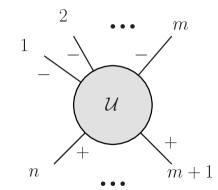
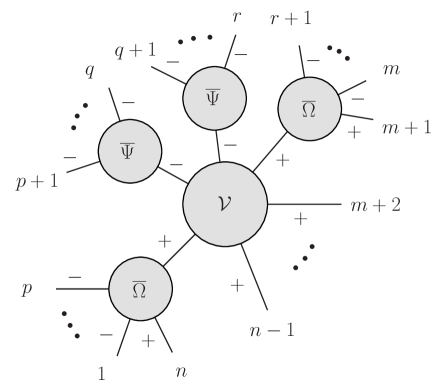
Figure 2: Left: color ordered vertex in the $Z$-field theory with $m$ minus helicity legs. Right: a general contribution to the $Z$-theory vertex. The central blob is the MHV vertex.

Specifically, consider now the vertex for $n$ external legs with the momenta $\mathbf{p}_{1}\dots\mathbf{p}_{n}$, where $\mathbf{p}_{1}\dots\mathbf{p}_{m}$ correspond to the minus helicity legs. Let us introduce a collective index $[i,i+1,\dots,j]$ labeling the momentum, $\mathbf{p}_{i(i+1)\dots j}=\mathbf{p}_{i}+\mathbf{p}_{i+1}+\dots+\mathbf{p}_{j}$. Using this notation, the general form of the color ordered vertex can be written as:

$$\mathcal{U}\left(1^{-},2^{-},\dots,m^{-},(m\!+\!1)^{+},\dots,n^{+}\right)=\sum_{p=0}^{m-2}\sum_{q=p+1}^{m-1}\sum_{r=q+1}^{m}\\ \mathcal{V}\left(\,[p\!+\!1,\dots,q]^{-},[q\!+\!1,\dots,r]^{-},[r\!+\!1,\dots,m\!+\!1]^{+},(m\!+\!2)^{+},\dots,(n\!-\!1)^{+},[n,1,\dots,p]^{+}\right)\\ \overline{\Omega}\left(n^{+},1^{-},\dots,p^{-}\right)\,\,\overline{\Psi}\left((p\!+\!1)^{-},\dots,q^{-}\right)\,\,\overline{\Psi}\left((q\!+\!1)^{-},\dots,r^{-}\right)\,\,\overline{\Omega}\left((r\!+\!1)^{-},\dots,m^{-},(m\!+\!1)^{+}\right)\,\,$$ (48)

Although the analytic formulas do not seem to collapse, in general, to any simple form, the above expression is operational and can be readily applied in the actual amplitude calculation, as we shall demonstrate in Section 3.

2.3 Summary: Feynman rules for the new action

Let us summarize the content of the new action. It contains a set of vertices with increasing multiplicity, starting at $n=4$. Each vertex has at least two minus helicity legs, and at most $n-2$. Thus, we have MHV vertices, next-to-MHV (NMHV) vertices, next-to-next-to-MHV (NNMHV) vertices and so on. The vertices with maximal number of minus helicity legs are just $\overline{\text{MHV}}$ vertices. Both the MHV and $\overline{\text{MHV}}$ vertices alone give the corresponding on-shell amplitudes. In addition to these vertices we have a scalar propagator joining two opposite helicity legs.

In the following section we shall demonstrate how various amplitudes are calculated. To this end we introduce the following color-ordered Feynman rules:

1. scalar propagator joining a plus and a minus helicity leg
   

   

2. $n$-point vertex, $n\geq 4$, with $m$ negative helicity legs, $2\leq m\leq n-2$
   

   

3 Applications

In this section we shall calculate several tree amplitudes using the new action.

3.1 4-point and 5-point amplitudes

The lowest non-zero amplitude is the 4-point MHV amplitude. It is simply given by the 4-point vertex in the theory.

The non-zero 5-point amplitudes are MHV $(--+++)$ and $\overline{\text{MHV}}$ $(---++)$. Both amplitudes are given just by a single vertex, respectively $\mathcal{U}(1^{-},2^{-},3^{+},4^{+},5^{+})$ and $\mathcal{U}(1^{-},2^{-},3^{-},4^{+},5^{+})$. For the MHV it is the expression (30), giving for the amplitude

$$\mathcal{A}(1^{-},2^{-},3^{+},4^{+},5^{+})=-g^{3}\left(\frac{p_{1}^{+}}{p_{2}^{+}}\right)^{2}\frac{\widetilde{v}_{21}^{*4}}{\widetilde{v}^{*}_{15}\widetilde{v}^{*}_{54}\widetilde{v}^{*}_{43}\widetilde{v}^{*}_{32}\widetilde{v}^{*}_{21}}\,.$$ (49)

For the $\overline{\text{MHV}}$ the expression is easily obtained from (48). In Fig. 3 we show the contributing terms. Using the explicit expressions we have:

$$\mathcal{U}(1^{-},2^{-},3^{-},4^{+},5^{+})=g^{3}\Bigg{[}\left(\frac{p_{1}^{+}}{p_{23}^{+}}\right)^{2}\frac{\widetilde{v}_{(23)1}^{*4}}{\widetilde{v}_{15}^{*}\widetilde{v}_{54}^{*}\widetilde{v}_{4(23)}^{*}\widetilde{v}_{({23})1}^{*}}\times\frac{{\widetilde{v}}_{({23})2}}{{\widetilde{v}}_{32}{\widetilde{v}}_{2({23})}}\\ +\left(\frac{p_{12}^{+}}{p_{3}^{+}}\right)^{2}\frac{\widetilde{v}_{3({12})}^{*4}}{\widetilde{v}_{({12}){5}}^{*}\widetilde{v}_{54}^{*}\widetilde{v}_{43}^{*}\widetilde{v}_{{3}({12})}^{*}}\times\frac{{\widetilde{v}}_{({12})1}}{{\widetilde{v}}_{21}{\widetilde{v}}_{1({12})}}\\ +\left(\frac{p_{2}^{+}}{p_{3}^{+}}\right)^{2}\frac{\widetilde{v}_{32}^{*4}}{\widetilde{v}_{2({15})}^{*}\widetilde{v}_{({15})4}^{*}\widetilde{v}_{43}^{*}\widetilde{v}_{32}^{*}}\times\left(\frac{p_{5}^{+}}{p_{15}^{+}}\right)^{2}\frac{{\widetilde{v}}_{({15})5}}{{\widetilde{v}}_{15}{\widetilde{v}}_{5({15})}}\\ +\left(\frac{p_{1}^{+}}{p_{2}^{+}}\right)^{2}\frac{\widetilde{v}_{21}^{*4}}{\widetilde{v}_{15}^{*}\widetilde{v}_{5\left(34\right)}^{*}\widetilde{v}_{({34)}2}^{*}\widetilde{v}_{21}^{*}}\times\left(\frac{p_{4}^{+}}{p_{34}^{+}}\right)^{2}\frac{{\widetilde{v}}_{({34})3}}{{\widetilde{v}}_{43}{\widetilde{v}}_{3({34})}}\Bigg{]}\,.$$ (50)

We have checked, that the above expression reduces in the on-shell limit to the known formula for the $\overline{\text{MHV}}$ amplitude:

$$\mathcal{A}(1^{-},2^{-},3^{-},4^{+},5^{+})=g^{3}\left(\frac{p_{4}^{+}}{p_{5}^{+}}\right)^{2}\frac{\widetilde{v}_{54}^{4}}{\widetilde{v}_{15}\widetilde{v}_{54}\widetilde{v}_{43}\widetilde{v}_{32}\widetilde{v}_{21}}\,.$$ (51)

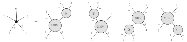
Figure 3: The contributions to the color-ordered $\overline{\text{MHV}}$ vertex, with helicity $(---++)$.

3.2 6-point amplitudes

The MHV and $\overline{\text{MHV}}$ amplitudes are always given by the single vertices. For the latter we need the $\mathcal{U}(1^{-},2^{-},3^{-},4^{-},5^{+},6^{+})$ vertex which is given by the formula (48), see Appendix B. We have verified that it recovers the correct result in the on-shell limit.

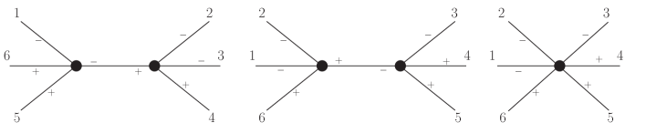
Figure 4: Diagrams contributing to the 6-point NMHV amplitude $(---+++)$.

The remaining amplitude is the NMHV amplitude with helicity configuration $(---+++)$. We have just three contributing diagrams depicted in Fig. 4. First two diagrams connect two MHV vertices, whereas the last one is the NMHV vertex, given by $\mathcal{U}(1^{-},2^{-},3^{-},4^{+},5^{+},6^{+})$. We have checked that the sum of those diagrams reproduce the known result in the on-shell limit [37].

3.3 7-point amplitudes

In addition to the MHV and $\overline{\text{MHV}}$ amplitudes, which are again calculated through just a single vertex, we have the NMHV and NNMHV amplitudes.

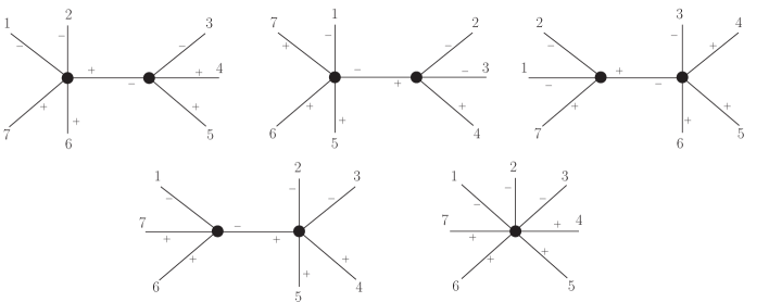
Figure 5: Diagrams contributing to the 7-point NMHV amplitude $(---++++)$.

The diagrams contributing to the NMHV amplitude are depicted in Fig. 5. We have four diagrams connecting 4-point and 5-point MHV vertices and one diagram which consists of the single vertex with NMHV helicity configuration. The corresponding expression is

$$D_{1}+D_{2}+D_{3}+D_{4}+\frac{1}{2}D_{5}\,,$$ (52)

where the individual diagrams are calculated as:

$$D_{1} =i\,\mathcal{U}\left(1^{-},2^{-},[3,4,5]^{+},6^{+},7^{+}\right)\times\frac{i}{p^{2}_{6712}}\times i\,\mathcal{U}\left([6,7,1,2]^{-},3^{-},4^{+},5^{+}\right)\,$$ (53)

$$D_{2} =i\,\mathcal{U}\left(1^{-},[2,3,4]^{-},5^{+},6^{+},7^{+}\right)\times\frac{i}{p^{2}_{234}}\times i\,\mathcal{U}\left(2^{-},3^{-},4^{+},[5,6,7,1]^{+}\right)\,$$ (54)

$$D_{3} =i\,\mathcal{U}\left(1^{-},2^{-},[3,4,5,6]^{+},7^{+}\right)\times\frac{i}{p^{2}_{3456}}\times i\,\mathcal{U}\left([7,1,2]^{-},3^{-},4^{+},5^{+},6^{+}\right)\,$$ (55)

$$D_{4} =i\,\mathcal{U}\left(1^{-},[2,3,4,5]^{-},6^{+},7^{+}\right)\times\frac{i}{p^{2}_{2345}}\times i\,\mathcal{U}\left(2^{-},3^{-},4^{+},5^{+},[6,7,1]^{+}\right)$$ (56)

$$D_{5} =i\,\mathcal{U}\left(1^{-},2^{-},3^{-},4^{+},5^{+},6^{+},7^{+}\right)\,.$$ (57)

In the above, $i/p^{2}_{i_{1}\dots i_{m}}=i/(p_{i_{1}}+\dots+p_{i_{m}})^{2}$ is the scalar propagator. The factor $1/2$ multiplying $D_{5}$ comes from the fact that there are two possible color orders contributing to diagrams $D_{1}$-$D_{4}$. We have compared the sum of those diagrams, i.e. Eq.(52) with the on-shell result obtained using the GGT Mathematica package [38] together with the S@M package [39] and found an exact match, up to an overall normalization due to the difference in our symbol $\tilde{v}_{ij}$ and $\left<ij\right>$.

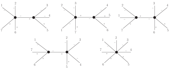
Figure 6: Diagrams contributing to the 7-point NNMHV amplitude $(----+++)$.

For the NNMHV amplitude the number of diagrams stays the same, see Fig. 6. Here, however, we encounter a new feature, namely there are now diagrams that connect the 4-point MHV vertex with 5-point $\overline{\text{MHV}}$ vertex. That is, starting with this amplitude we utilize the new vertices appearing in the theory in a nontrivial way (i.e. by gluing them with other vertices). We again find the on shell limit of the result consistent with the GGT package.

3.4 8-point amplitudes

We have also calculated some of the non-trivial 8-point amplitudes, all of which agree with the standard results calculated numerically using the GGT package.

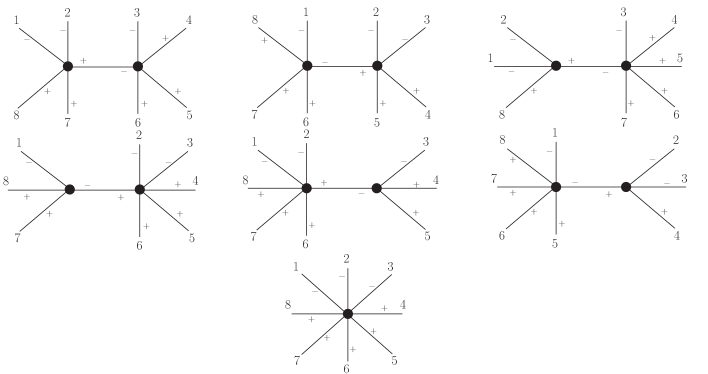
Figure 7: Diagrams contributing to the 8-point NMHV amplitude $(---+++++)$.

The 8-point NMHV amplitude turns out to be actually very simple, requiring only 7 diagrams, of which 6 join two MHV vertices, see Fig. 7.

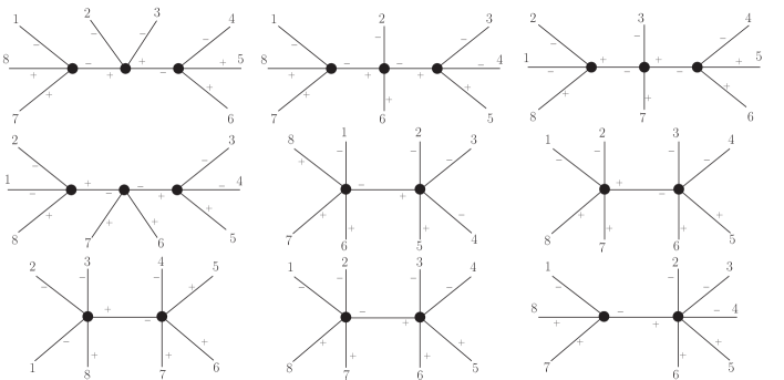
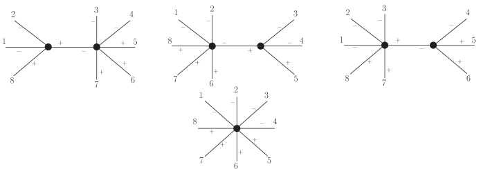
Figure 8: Diagrams contributing to the 8-point NNMHV amplitude $(----++++)$.

In order to really test the new theory we calculated the 8-point NNMHV amplitude. In that case, we encounter only 13 diagrams, shown in Fig. 8, of which some consist of three MHV vertices joined by the scalar propagators, but there are also diagrams combining the 5-point $\overline{\text{MHV}}$ vertex as well as 6-point NMHV vertex appearing in the $Z$-field theory. As this calculation is less trivial, let us list the structure of the diagrams (they correspond to the diagrams in Fig. 8 from the top left, going to the right):

$$D_{1}=i\,\mathcal{U}\left([7,8,1,2,3]^{-},4^{-},5^{+},6^{+}\right)\times\frac{i}{p^{2}_{456}}\times i\,\mathcal{U}\left(1^{-},[2,3,4,5,6]^{-},7^{+},8^{+}\right)\\ \times\frac{i}{p^{2}_{781}}\times i\,\mathcal{U}\left(2^{-},3^{-},[4,5,6]^{+},[7,8,1]^{+}\right)\,,$$ (58)

$$D_{2}=i\,\mathcal{U}\left(3^{-},4^{-},5^{+},[6,7,8,1,2]^{+}\right)\times\frac{i}{p^{2}_{67812}}\times i\,\mathcal{U}\left(1^{-},[2,3,4,5,6]^{-},7^{+},8^{+}\right)\\ \times\frac{i}{p^{2}_{781}}\times i\,\mathcal{U}\left(2^{-},[3,4,5,]^{-},6^{+},[7,8,1]^{+}\right)\,,$$ (59)

$$D_{3}=i\,\mathcal{U}\left([7,8,1,2,3]^{-},4^{-},5^{+},6^{+}\right\}\times\frac{i}{p^{2}_{456}}\times i\,\mathcal{U}\left(1^{-},2^{-},[3,4,5,6,7]^{+},8^{+}\right)\\ \times\frac{i}{p^{2}_{812}}\times i\,\mathcal{U}\left([8,1,2]^{-},3^{-},[4,5,6]^{+},7^{+}\right)\,,$$ (60)

$$D_{4}=i\,\mathcal{U}\left(3^{-},4^{-},5^{+},[6,7,8,1,2]^{+}\right)\times\frac{i}{p^{2}_{67812}}\times i\,\mathcal{U}\left(1^{-},2^{-},[3,4,5,6,7]^{+},8^{+}\right)\\ \times\frac{i}{p^{2}_{812}}\times i\,\mathcal{U}\left([8,1,2]^{-},[3,4,5]^{-},6^{+},7^{+}\right)\,,$$ (61)

$$D_{5}=i\,\mathcal{U}\left(1^{-},[2,3,4,5]^{-},6^{+},7^{+},8^{+}\right)\times\frac{i}{p^{2}_{2345}}\times i\,\mathcal{U}\left(2^{-},3^{-},4^{-},5^{+},[6,7,8,1]\right)\,,$$ (62)

$$D_{6}=i\,\mathcal{U}\left(1^{-},2^{-},[3,4,5,6]^{+},7^{+},8^{+}\right)\times\frac{i}{p^{2}_{3456}}\times i\,\mathcal{U}\left([7,8,1,2]^{-},3^{-},4^{-},5^{+},6^{+}\right)\,,$$ (63)

$$D_{7}=i\,\mathcal{U}\left(1^{-},2^{-},3^{-},[4,5,6,7]^{+},8^{+}\right)\times\frac{i}{p^{2}_{4567}}\times i\,\mathcal{U}\left([8,1,2,3]^{-},4^{-},5^{+},6^{+},7^{+}\right)\,,$$ (64)

$$D_{8}=i\,\mathcal{U}\left(1^{-},2^{-},[3,4,5,6]^{-},7^{+},8^{+}\right)\times\frac{i}{P^{2}_{3456}}\times i\,\mathcal{U}\left(3^{-},4^{-},5^{+},6^{+},[7,8,1,2]^{+}\right)\,,$$ (65)

$$D_{9}=i\,\mathcal{U}\left(1^{-},[2,3,4,5,6]^{-},7^{+},8^{+}\right)\times\frac{i}{p^{2}_{23456}}\times i\,\mathcal{U}\left(2^{-},3^{-},4^{-},5^{+},6^{+},[7,8,1]^{+}\right)\,,$$ (66)

$$D_{10}=i\,\mathcal{U}\left(1^{-},2^{-},[3,4,5,6,7]^{+},8^{+}\right\}\times\frac{i}{p^{2}_{34567}}\times i\,\mathcal{U}\left([8,1,2]^{-},3^{-},4^{-},5^{+},6^{+},7^{+}\right)\,,$$ (67)

$$D_{11}=i\,\mathcal{U}\left(3^{-},4^{-},5^{+},[6,7,8,1,2]^{+}\right)\times\frac{i}{p^{2}_{67812}}\times i\,\mathcal{U}\left(1^{-},2^{-},[3,4,5]^{-},6^{+},7^{+},8^{+}\right)\,,$$ (68)

$$D_{12}=i\,\mathcal{U}\left([7,8,1,2,3]^{-},4^{-},5^{+},6^{+}\right)\times\frac{i}{p^{2}_{456}}\times i\,\mathcal{U}\left(1^{-},2^{-},3^{-},[4,5,6]^{+},7^{+},8^{+}\right)\,,$$ (69)

$$D_{13}=i\,\mathcal{U}\left(1^{-},2^{-},3^{-},4^{-},5^{+},6^{+},7^{+},8^{+}\right)\,.$$ (70)

The above diagrams have to be combined as follows, due to the additional combinatorial factors as explained in the previous subsection:

$$D_{1}+D_{2}+D_{3}+D_{4}+\frac{1}{2}\left(D_{5}+D_{6}+D_{7}+D_{8}+D_{9}+D_{10}+D_{11}+D_{12}\right)+\frac{1}{4}D_{13}\,.$$ (71)

4 Discussion

# legs	helicity	# diagrams
4 point	$\mathrm{MHV}$	1
	$\mathrm{\overline{MHV}}$	1
5 point	$\mathrm{MHV}$	1
	$\mathrm{\overline{MHV}}$	1
6 point	$\mathrm{MHV}$	1
	$\mathrm{NMHV}$	3
	$\mathrm{\overline{MHV}}$	1
7 point	$\mathrm{MHV}$	1
	$\mathrm{NMHV}$	5
	$\mathrm{NNMHV}$	5
	$\mathrm{\overline{MHV}}$	1
8 point	$\mathrm{MHV}$	1
	$\mathrm{NMHV}$	7
	$\mathrm{NNMHV}$	13
	$\mathrm{NNNMHV}$	7
	$\mathrm{\overline{MHV}}$	1

Table 1: Total number of diagrams for helicity amplitudes of different multiplicities.

In the present work we have constructed a new action for gluodynamics by applying two consecutive canonical transformations on the light-cone Yang-Mills action, see Fig. 1. The same action can be also obtained by a single canonical transformation, whose generating functional is given by Eq. (6).

The most striking property of the new action is that it has no triple-gluon vertex. Effectively, the triple-gluon vertices are resummed inside the Wilson lines (see [27] for the explicit demonstration of that fact for the $(++-)$ vertex). Consequently, the number of diagrams needed to calculate the amplitudes is reduced, as compared for example to the CSW method. For example, for the NMHV amplitudes with adjacent helicity, the CSW rules give $2(n-3)$ diagrams, whereas the new theory gives $2(n-5)+1$ diagrams, $n\geq 5$. We give the number of diagrams for various adjacent helicity configurations in Table 1. It is important to stress, that we do not mean here the number of contributing terms, as the vertices in the new theory are not, in general, given by a single term in our representation. The structure of those vertices can be however easily obtained by means of the master equation (48).

One of the very interesting aspects of the field transformations leading to the new action is its incredibly rich geometric structure. Let us recall, that the new minus helicity field $Z^{\star}$ is given by the straight infinite Wilson line on the anti-self-dual plane (i.e. the plane spanned by $\varepsilon_{\perp}^{-}$ and $\eta$), integrated over all directions. This is the Wilson line functional of the minus helicity field of the MHV theory, which itself is given as the analogous Wilson line of the usual gauge fields lying on the self-dual plane, with insertion of the minus helicity field (i.e. the functional derivative, see Eq. (32)). We schematically depict the structure of the $Z^{\star}$ field in Fig. 9. A similar figure can be drawn for the $Z^{\bullet}$ field. We stress, that although the overall picture looks very non-local, it is local in the light-cone time.

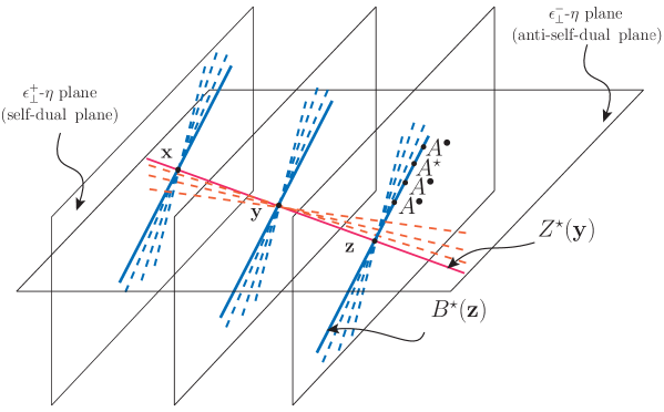
Figure 9: Schematic presentation of the geometric structure of the $Z^{\star}$ field (the structure of $Z^{\bullet}$ is quite similar). The vertical planes are the self-dual planes, i.e. the planes spanned by the vectors $\varepsilon_{\perp}^{+}=(0,1,i,0)$ and $\eta=(1,0,0,-1)$. The horizontal plane, in our terminology, is the anti-self-dual plane, i.e. it is spanned by $\varepsilon_{\perp}^{-}=(0,1,-i,0)$ and $\eta$. The $B^{\star}$ fields (the minus helicity fields in the MHV action) are the straight infinite Wilson lines on the self-dual plane, integrated over all slopes, and differentiated functionally to replace one plus gluon helicity field by the minus gluon helicity field. This structure is represented by the blue lines. The $Z^{\star}$ field, i.e. the minus helicity field in the new theory, is given by a similar Wilson line of the $B^{\star}$ fields, lying on the anti-self dual plane, and integrated over all slopes.

In our recent work [28] we have discussed the fields in the MHV theory, where the fields can be expressed as the Wilson line functionals of the standard gauge fields lying exclusively on the self-dual plane. We see that the transformations derived in the present work extend this picture to the whole 3-space, with the light-cone time fixed.

One of the future directions is obviously to find the quantum corrections to the new action. There is an immediate difficulty in that program, namely, the fact that in the quantum MHV action there are contributions evading the S-matrix equivalence theorem [17], and we expect similar contributions in the new action. An alternative approach is based on the world-sheet regularization, which successfully recovered one loop all-plus helicity vertex in the MHV action [19].

Another interesting direction of future study is related to the rich geometric structure of the transformations, sketched in Fig. 9, which has not been fully explored.

5 Acknowledgments

H.K. and P.K. are supported by the National Science Centre, Poland grant no. 2018/31/D/ST2/02731. A.M.S. is supported by the U.S. Department of Energy Grant DE-SC-0002145 and in part by National Science Centre in Poland, grant 2019/33/B/ST2/02588.

Appendix A Cancellation of triple-gluon vertices.

In this appendix we show the cancellation of both the triple-gluon vertices when transforming the Yang-Mills fields to the new fields,

$$\left\{\hat{A}^{\bullet},\hat{A}^{\star}\right\}\rightarrow\Big{\{}\hat{Z}^{\bullet}\big{[}{A}^{\bullet},{A}^{\star}\big{]},\hat{Z}^{\star}\big{[}{A}^{\bullet},{A}^{\star}\big{]}\Big{\}}\,.$$ (72)

As previously argued, there are two ways of doing this: using directly the generating functional (7), or using two consecutive canonical field transformations. For convenience, we shall follow the second path. So the strategy is to express $A$ fields in terms of $B$ fields and then substitute for $B$ fields in terms of $Z$ fields. Then we shall substitute the $A$ fields (expressed already in terms of $Z$ fields up to the second order) into the standard Yang-Mills action (3) to show that the triple-gluon vertices cancel out.

Using the relations (17)-(18) and (41)-(43), it is easy to see that the expansion of $\widetilde{A}^{\bullet}$, $\widetilde{A}^{\star}$ fields, to second order in $\widetilde{Z}$ fields is the following:

$$\Big{[}{\widetilde{A}}^{\bullet}_{a}(x^{+};\mathbf{P})\Big{]}_{2nd}=\int\!d^{3}\mathbf{p}_{1}d^{3}\mathbf{p}_{2}\,\overline{\widetilde{\Omega}}\,^{ab_{1}\left\{b_{2}\right\}}_{2}(\mathbf{P};\mathbf{p_{1}},\left\{\mathbf{p_{2}}\right\}){\widetilde{Z}}^{\bullet}_{b_{1}}(x^{+};\mathbf{p}_{1}){\widetilde{Z}}^{\star}_{b_{2}}(x^{+};\mathbf{p}_{2})\\ +\int\!d^{3}\mathbf{p}_{1}\,d^{3}\mathbf{p}_{2}{\widetilde{\Psi}}_{2}^{a\left\{b_{1}b_{2}\right\}}(\mathbf{P};\left\{\mathbf{p}_{1},\mathbf{p}_{2}\right\}){\widetilde{Z}}^{\bullet}_{b_{1}}(x^{+};\mathbf{p}_{1}){\widetilde{Z}}^{\bullet}_{b_{2}}(x^{+};\mathbf{p}_{2})\,,$$ (73)

and

$$\Big{[}{\widetilde{A}}^{\star}_{a}(x^{+};\mathbf{P})\Big{]}_{2nd}=\int\!d^{3}\mathbf{p}_{1}\,d^{3}\mathbf{p}_{2}\,\overline{\Psi}\,^{a\{b_{1}b_{2}\}}_{2}(\mathbf{P};\{\mathbf{p}_{1},\mathbf{p}_{2}\}){\widetilde{Z}}^{\star}_{b_{1}}(x^{+};\mathbf{p}_{1}){\widetilde{Z}}^{\star}_{b_{2}}(x^{+};\mathbf{p}_{2})\\ +\int\!d^{3}\mathbf{p}_{1}\,d^{3}\mathbf{p}_{2}\,{\widetilde{\Omega}}_{2}^{ab_{1}\left\{b_{2}\right\}}(\mathbf{P};\mathbf{p}_{1},\left\{\mathbf{p}_{2}\right\}){\widetilde{Z}}^{\star}_{b_{1}}(x^{+};\mathbf{p}_{1}){\widetilde{Z}}^{\bullet}_{b_{2}}(x^{+};\mathbf{p}_{2})\,.$$ (74)

The above kernels represent the momentum space version of $\Xi_{1,1}^{ab_{1}b_{2}}(\mathbf{x};\mathbf{y}_{1},\mathbf{y}_{2})$, $\Xi_{2,0}^{ab_{1}b_{2}}(\mathbf{x};\mathbf{y}_{1},\mathbf{y}_{2})$, $\Lambda_{2,0}^{ab_{1}b_{2}}(\mathbf{x};\mathbf{y}_{1},\mathbf{y}_{2})$ and $\Lambda_{1,1}^{ab_{1}b_{2}}(\mathbf{x};\mathbf{y}_{1},\mathbf{y}_{2})$ respectively, introduced in Eqs. (10)-(11). All the above relations are three dimensional Fourier transforms performed for a fixed light-come time $x^{+}$. Since the kernels are independent of the minus component of momentum $k^{-}$, the four dimensional transforms will only account for an extra delta function for the minus component conservation.

In momentum space, the kinetic and triple-gluon terms of the Yang-Mills action (3) read

$$\mathcal{L}_{+-}^{\left(\mathrm{LC}\right)}=\int d^{4}{p}_{1}d^{4}{p}_{2}\,\delta^{4}\left({p}_{1}+{p}_{2}\right)\,{p}_{1}^{2}\,\,\widetilde{A}_{a}^{\bullet}\left({p}_{1}\right)\widetilde{A}_{a}^{\star}\left({p}_{2}\right)\,,$$ (75)

$$\mathcal{L}_{++-}^{\left(\mathrm{LC}\right)}=\int d^{3}\mathbf{p}_{1}d^{3}\mathbf{p}_{2}d^{3}\mathbf{p}_{3}\,\delta^{3}\left(\mathbf{p}_{1}+\mathbf{p}_{2}+\mathbf{p}_{3}\right)\widetilde{V}_{++-}^{abc}\left(\mathbf{p}_{1},\mathbf{p}_{2},\mathbf{p}_{3}\right)\,\\ \widetilde{A}_{a}^{\bullet}\left(x^{+};\mathbf{p}_{1}\right)\widetilde{A}_{b}^{\bullet}\left(x^{+};\mathbf{p}_{2}\right)\widetilde{A}_{c}^{\star}\left(x^{+};\mathbf{p}_{3}\right)\,,$$ (76)

with the helicity triple-gluon vertex

$$\widetilde{V}_{++-}^{abc}\left(\mathbf{p}_{1},\mathbf{p}_{2},\mathbf{p}_{3}\right)=-igf^{abc}\left(\frac{p_{1}^{\star}}{p_{1}^{+}}-\frac{p_{2}^{\star}}{p_{2}^{+}}\right)p_{3}^{+}\,$$ (77)

and

$$\mathcal{L}_{--+}^{\left(\mathrm{LC}\right)}=\int d^{3}\mathbf{p}_{1}d^{3}\mathbf{p}_{2}d^{3}\mathbf{p}_{3}\,\delta^{3}\left(\mathbf{p}_{1}+\mathbf{p}_{2}+\mathbf{p}_{3}\right)\widetilde{V}_{--+}^{abc}\left(\mathbf{p}_{1},\mathbf{p}_{2},\mathbf{p}_{3}\right)\,\\ \widetilde{A}_{a}^{\star}\left(x^{+};\mathbf{p}_{1}\right)\widetilde{A}_{b}^{\star}\left(x^{+};\mathbf{p}_{2}\right)\widetilde{A}_{c}^{\bullet}\left(x^{+};\mathbf{p}_{3}\right)\,,$$ (78)

with

$$\widetilde{V}_{--+}^{abc}\left(\mathbf{p}_{1},\mathbf{p}_{2},\mathbf{p}_{3}\right)=-igf^{abc}\left(\frac{p_{1}^{\bullet}}{p_{1}^{+}}-\frac{p_{2}^{\bullet}}{p_{2}^{+}}\right)p_{3}^{+}\,.$$ (79)

Above, we have used the 3-dimensional Fourier transform at a constant light-cone time $x^{+}$ for the interaction terms, and the full 4 dimensional Fourier transform for the kinetic term, because the inverse propagator acts also on the light-cone time (i.e. it contains $\partial_{+}$ operator). Since the triple-gluon vertices are independent of $x^{+}$, we can directly substitute the $A$ fields in term of $Z$ fields, at a constant $x^{+}$ time.

In order to deal with the kinetic term, we need (73) and (74) written fully in momentum space. As mentioned, this is straightforward and accounts for a minus momentum component conservation delta in the kernels. We have, up to the third order in $Z$ fields,

$$\mathcal{L}_{+-}=\int d^{4}{p}_{1}d^{4}{p}_{2}\,\delta^{4}\left({p}_{1}+{p}_{2}\right)\,{p}_{1}^{2}\,\,\Bigg{\{}\Bigg{[}\int\!d^{4}{q}_{1}d^{4}{q}_{2}\,\,\overline{\widetilde{\Omega}}\,^{ac_{1}\left\{c_{2}\right\}}_{2}({p}_{1};{q}_{1},\left\{{q}_{2}\right\})\\ \times{\widetilde{Z}}^{\bullet}_{c_{1}}({q}_{1}){\widetilde{Z}}^{\star}_{c_{2}}({q}_{2})+{\widetilde{\Psi}}_{2}^{a\left\{c_{1}c_{2}\right\}}({p}_{1};\left\{{q}_{1},{q}_{2}\right\}){\widetilde{Z}}^{\bullet}_{c_{1}}({q}_{1}){\widetilde{Z}}^{\bullet}_{c_{2}}({q}_{2})\,\Bigg{]}\widetilde{Z}_{a}^{\star}\left({p}_{2}\right)\,\\ +\widetilde{Z}_{a}^{\bullet}\left({p}_{1}\right)\times\Bigg{[}\int\!d^{4}{q}_{1}\,d^{4}{q}_{2}\,\,\overline{\Psi}\,^{a\left\{c_{1}c_{2}\right\}}_{2}({p}_{2};\left\{{q}_{1},{q}_{2}\right\}){\widetilde{Z}}^{\star}_{c_{1}}({q}_{1}){\widetilde{Z}}^{\star}_{c_{2}}({q}_{2})\\ +{\widetilde{\Omega}}_{2}^{ac_{1}\left\{c_{2}\right\}}({p}_{2};{q}_{1},\left\{{q}_{2}\right\}){\widetilde{Z}}^{\star}_{c_{1}}({q}_{1}){\widetilde{Z}}^{\bullet}_{c_{2}}({q}_{2})\Bigg{]}\Bigg{\}}\,.$$ (80)

Let us first consider the terms that have (${\widetilde{Z}^{\star}}{\widetilde{Z}^{\star}}{\widetilde{Z}^{\bullet}}$) field configuration:

$$\mathcal{T}_{--+}=\int d^{4}{p}_{1}d^{4}{p}_{2}\,\delta^{4}\left({p}_{1}+{p}_{2}\right)\,{p}_{1}^{2}\,\,\Bigg{[}\int\!d^{4}{q}_{1}d^{4}{q}_{2}\,\,\overline{\widetilde{\Omega}}\,^{ac_{1}\left\{c_{2}\right\}}_{2}({p}_{1};{q}_{1},\left\{{q}_{2}\right\})\\ \times{\widetilde{Z}}^{\bullet}_{c_{1}}({q}_{1}){\widetilde{Z}}^{\star}_{c_{2}}({q}_{2})\widetilde{Z}_{a}^{\star}\left({p}_{2}\right)\,+\widetilde{Z}_{a}^{\bullet}\left({p}_{1}\right)\int\!d^{4}{q}_{1}\,d^{4}{q}_{2}\,\,\overline{\widetilde{\Psi}}\,^{a\left\{c_{1}c_{2}\right\}}_{2}({p}_{2};\left\{{q}_{1},{q}_{2}\right\}){\widetilde{Z}}^{\star}_{c_{1}}({q}_{1}){\widetilde{Z}}^{\star}_{c_{2}}({q}_{2})\Bigg{]}\,.$$ (81)

Integrating the first and second term over $p_{1}$ and $p_{2}$ respectively, we see that each term will have only three momentum variables. Both terms can be combined into one integral by renaming the momentum variables to $p_{1},p_{2},p_{3}$, and color indices to $b_{1}$, $b_{2}$, $b_{3}$. With this we have

$$\mathcal{T}_{--+}=\int d^{4}{p}_{1}d^{4}{p}_{2}d^{4}{p}_{3}\,\Bigg{[}{p}_{2}^{2}\,\,\overline{\widetilde{\Omega}}\,^{b_{2}b_{3}\left\{b_{1}\right\}}_{2}(-{p}_{2};{p}_{3},\left\{{p}_{1}\right\})\\ +{p}_{3}^{2}\overline{\widetilde{\Psi}}\,^{b_{3}\left\{b_{1}b_{2}\right\}}_{2}(-{p}_{3};\left\{{p}_{1},{p}_{2}\right\})\Bigg{]}{\widetilde{Z}}^{\star}_{b_{1}}({p}_{1}){\widetilde{Z}}^{\star}_{b_{2}}({p}_{2})\widetilde{Z}_{b_{3}}^{\bullet}\left({p}_{3}\right)\,.$$ (82)

In order to bring the above expression to the constant light cone time $x^{+}$ we introduce the following auxiliary fields (both for $\widetilde{Z}^{\bullet}$ and $\widetilde{Z}^{\star}$)

$${\widetilde{Z}}_{b_{i}}(p_{i})=\frac{{\widetilde{\kappa}}_{b_{i}}(p_{i})}{p_{i}^{2}}\,.$$ (83)

Substituting (83) in (82) we obtain

$$\mathcal{T}_{--+}=\int d^{4}{p}_{1}d^{4}{p}_{2}d^{4}{p}_{3}\,\Bigg{[}{p}_{2}^{2}\,\,\overline{\widetilde{\Omega}}\,^{b_{2}b_{3}\left\{b_{1}\right\}}_{2}(-{p}_{2};{p}_{3},\left\{{p}_{1}\right\})\\ +{p}_{3}^{2}\overline{\widetilde{\Psi}}\,^{b_{3}\left\{b_{1}b_{2}\right\}}_{2}(-{p}_{3};\left\{{p}_{1},{p}_{2}\right\})\Bigg{]}\frac{{\widetilde{\kappa}}^{\star}_{b_{1}}(p_{1})}{p_{1}^{2}}\frac{{\widetilde{\kappa}}^{\star}_{b_{2}}(p_{2})}{p_{2}^{2}}\frac{{\widetilde{\kappa}}^{\bullet}_{b_{3}}(p_{3})}{p_{3}^{2}}\,.$$ (84)

Next, we integrate out the minus momentum components. To this end, the first term in (84) can be rewritten as

$$\int d^{3}\mathbf{p}_{1}d^{3}\mathbf{p}_{2}d^{3}\mathbf{p}_{3}\,\,\int dp_{1}^{-}\,dp_{2}^{-}\ dp_{3}^{-}dP^{-}\,\int dz^{+}\int dy^{+}e^{iz^{+}(P^{-}-p_{2}^{-})}\,\,e^{iy^{+}(P^{-}+p_{1}^{-}+p_{3}^{-})}(-p_{13}^{+})(P^{-}+\hat{p}_{13})\\ \overline{\widetilde{\Omega}}\,^{b_{2}b_{3}\left\{b_{1}\right\}}_{2}(-\mathbf{p}_{2};\mathbf{p}_{3},\left\{\mathbf{p}_{1}\right\})\frac{1}{2p_{1}^{+}[p_{1}^{-}-\hat{p}_{1}+i\epsilon]}\frac{1}{2p_{2}^{+}[p_{2}^{-}-\hat{p}_{2}+i\epsilon]}\\ \frac{1}{2p_{3}^{+}[p_{3}^{-}-\hat{p}_{3}+i\epsilon]}{\widetilde{\kappa}}^{\star}_{b_{1}}(p_{1}){\widetilde{\kappa}}^{\star}_{b_{2}}(p_{2}){\widetilde{\kappa}}^{\star}_{b_{3}}(p_{3})\,.$$ (85)

where we introduced the notation

$$\hat{p}=\frac{p^{\bullet}p^{\star}}{p^{+}}\,,$$ (86)

for any momentum $p$. This leads to

$$\int d^{3}\mathbf{p}_{1}d^{3}\mathbf{p}_{2}d^{3}\mathbf{p}_{3}\,\,\,p_{13}^{+}(\hat{p}_{1}+\hat{p}_{3}-\hat{p}_{13})\,\,\overline{\widetilde{\Omega}}\,^{b_{2}b_{3}\left\{b_{1}\right\}}_{2}(-\mathbf{p}_{2};\mathbf{p}_{3},\left\{\mathbf{p}_{1}\right\})\frac{{(i\pi)}^{3}}{p_{1}^{+}p_{2}^{+}p_{3}^{+}}\\ \times\Bigg{[}\prod_{i=1}^{3}\Theta(-p_{i}^{+})\frac{i}{\hat{p}_{1}+\hat{p}_{2}+\hat{p}_{3}+i\epsilon}+\prod_{i=1}^{3}\Theta(p_{i}^{+}){(-1)}^{3}\frac{-i}{\hat{p}_{1}+\hat{p}_{2}+\hat{p}_{3}+i\epsilon}\Bigg{]}\\ \times{\widetilde{\kappa}}^{\star}_{b_{1}}\left(\hat{p}_{1};\mathbf{p}_{1}\right){\widetilde{\kappa}}^{\star}_{b_{2}}\left(\hat{p}_{2};\mathbf{p}_{2}\right){\widetilde{\kappa}}^{\star}_{b_{3}}\left(\hat{p}_{3};\mathbf{p}_{3}\right)\,,$$ (87)

where $\Theta(p_{i}^{+})$ is Heaviside step function. This may be rewritten as

$$\int dx^{+}\,\int d^{3}\mathbf{p}_{1}d^{3}\mathbf{p}_{2}d^{3}\mathbf{p}_{3}\,\,\,p_{13}^{+}(\hat{p}_{1}+\hat{p}_{3}-\hat{p}_{13})\,\,\overline{\widetilde{\Omega}}\,^{b_{2}b_{3}\left\{b_{1}\right\}}_{2}(-\mathbf{p}_{2};\mathbf{p}_{3},\left\{\mathbf{p}_{1}\right\})\\ \times{\widetilde{Z}}^{\star}_{b_{1}}(x^{+};\mathbf{p}_{1}){\widetilde{Z}}^{\star}_{b_{2}}(x^{+};\mathbf{p}_{2})\widetilde{Z}_{b_{3}}^{\bullet}\left(x^{+};\mathbf{p}_{3}\right)\,,$$ (88)

where, in going from (87) to (88), we used the following relation

$$\int dx^{+}\,\int d^{3}\mathbf{p}_{1}\cdots d^{3}\mathbf{p}_{n}\,\,\,{\widetilde{f}}(\mathbf{p}_{1}\cdots\mathbf{p}_{n}){\widetilde{Z}}^{\star}_{b_{1}}(x^{+};\mathbf{p}_{1})\cdots\widetilde{Z}_{b_{n}}^{\bullet}\left(x^{+};\mathbf{p}_{n}\right)\\ =\int d^{3}\mathbf{p}_{1}\cdots d^{3}\mathbf{p}_{n}\,\,\,{\widetilde{f}}(\mathbf{p}_{1}\cdots\mathbf{p}_{n})\frac{{(i\pi)}^{n}}{p_{1}^{+}\cdots p_{n}^{+}}\Bigg{[}\prod_{i=1}^{n}\Theta(-p_{i}^{+})\frac{i}{\hat{p}_{1}+\cdots+\hat{p}_{n}+i\epsilon}\\ +\prod_{i=1}^{n}\Theta(p_{i}^{+}){(-1)}^{n}\frac{-i}{\hat{p_{1}}+\cdots+\hat{p_{n}}+i\epsilon}\Bigg{]}{\widetilde{\kappa}}^{\star}_{b_{1}}\left(\hat{p}_{1};\mathbf{p}_{1}\right)\cdots{\widetilde{\kappa}}^{\star}_{b_{n}}\left(\hat{p}_{n};\mathbf{p}_{n}\right)\,.$$ (89)

Above, ${\widetilde{f}}(\mathbf{p}_{1}\cdots\mathbf{p}_{n})$ represents any generic function not depending on the minus momentum components (or the light-cone time). In a similar way, the second term in (84) gives

$$\int dx^{+}\,\int d^{3}\mathbf{p}_{1}d^{3}\mathbf{p}_{2}d^{3}\mathbf{p}_{3}\,\,\,p_{12}^{+}(\hat{p}_{1}+\hat{p}_{2}-\hat{p}_{12})\overline{\widetilde{\Psi}}\,^{b_{3}\left\{b_{1}b_{2}\right\}}_{2}(-\mathbf{p}_{3};\left\{\mathbf{p}_{1},\mathbf{p}_{2}\right\})\\ \times{\widetilde{Z}}^{\star}_{b_{1}}(x^{+};\mathbf{p}_{1}){\widetilde{Z}}^{\star}_{b_{2}}(x^{+};\mathbf{p}_{2})\widetilde{Z}_{b_{3}}^{\bullet}\left(x^{+};\mathbf{p}_{3}\right)\,.$$ (90)

Combining Eq. (88) and (90) we get

$$\mathcal{T}_{--+}=\int dx^{+}\,\int d^{3}\mathbf{p}_{1}d^{3}\mathbf{p}_{2}d^{3}\mathbf{p}_{3}\,\Bigg{[}p_{13}^{+}(\hat{p}_{1}+\hat{p}_{3}-\hat{p}_{13})\,\,\overline{\widetilde{\Omega}}\,^{b_{2}b_{3}\left\{b_{1}\right\}}_{2}(-\mathbf{p}_{2};\mathbf{p}_{3},\left\{\mathbf{p}_{1}\right\})\\ +p_{12}^{+}(\hat{p}_{1}+\hat{p}_{2}-\hat{p}_{12})\,\,\overline{\widetilde{\Psi}}\,^{b_{3}\left\{b_{1}b_{2}\right\}}_{2}(-\mathbf{p}_{3};\left\{\mathbf{p}_{1},\mathbf{p}_{2}\right\})\Bigg{]}{\widetilde{Z}}^{\star}_{b_{1}}(x^{+};\mathbf{p}_{1}){\widetilde{Z}}^{\star}_{b_{2}}(x^{+};\mathbf{p}_{2})\widetilde{Z}_{b_{3}}^{\bullet}\left(x^{+};\mathbf{p}_{3}\right)\,.$$ (91)

Using $p_{ij}^{+}(\hat{p_{i}}+\hat{p_{j}}-\hat{p_{ij}})=-{\widetilde{v}}_{(i)(j)}{\widetilde{v}}^{\ast}_{(j)(i)}$ and substituting for $\overline{\widetilde{\Omega}}$ and $\overline{\widetilde{\Psi}}$ the kernels from (44) and (42), respectively, after a bit of algebra we obtain

$$\mathcal{T}_{--+}=\int dx^{+}\,\int d^{3}\mathbf{p}_{1}d^{3}\mathbf{p}_{2}d^{3}\mathbf{p}_{3}\,\delta^{3}\left(\mathbf{p}_{1}+\mathbf{p}_{2}+\mathbf{p}_{3}\right)\\ \times\Big{(}igf^{b_{1}b_{2}b_{3}}p_{3}^{+}{v}^{\ast}_{12}\Big{)}\times{\widetilde{Z}}^{\star}_{b_{1}}(x^{+};\mathbf{p}_{1}){\widetilde{Z}}^{\star}_{b_{2}}(x^{+};\mathbf{p}_{2})\widetilde{Z}_{b_{3}}^{\bullet}\left(x^{+};\mathbf{p}_{3}\right)\,,$$ (92)

where $\widetilde{v}_{ij}=p_{i}^{+}v_{ji}$. Comparing this with (79), we may rewrite the above as

$$\mathcal{T}_{--+}=\int dx^{+}\,\int d^{3}\mathbf{p}_{1}d^{3}\mathbf{p}_{2}d^{3}\mathbf{p}_{3}\,\delta^{3}\left(\mathbf{p}_{1}+\mathbf{p}_{2}+\mathbf{p}_{3}\right)\\ \times\Big{(}-\widetilde{V}_{--+}^{b_{1}b_{2}b_{3}}\left(\mathbf{p}_{1},\mathbf{p}_{2},\mathbf{p}_{3}\right)\Big{)}\times{\widetilde{Z}}^{\star}_{b_{1}}(x^{+};\mathbf{p}_{1}){\widetilde{Z}}^{\star}_{b_{2}}(x^{+};\mathbf{p}_{2})\widetilde{Z}_{b_{3}}^{\bullet}\left(x^{+};\mathbf{p}_{3}\right)\,.$$ (93)

This cancels out the triple-gluon vertex coming from the Yang-Mills action (78) when we substitute the first order expansion of $\widetilde{A}^{\bullet}$ and $\widetilde{A}^{\star}$ in terms of $\widetilde{Z}^{\bullet}$ and $\widetilde{Z}^{\star}$ fields.

In exactly same fashion, the cancellation of the other triple-gluon vertex $\widetilde{V}_{++-}^{b_{1}b_{2}b_{3}}\left(\mathbf{p}_{1},\mathbf{p}_{2},\mathbf{p}_{3}\right)$ can be shown.

Appendix B Six point $\overline{\mathrm{MHV}}$ amplitude.

In this appendix we show the details associated with the calculation of the 6-point $\overline{\mathrm{MHV}}$ $(----++)$ amplitude. As mentioned previously, the $\overline{\text{MHV}}$ amplitudes are always given by a single vertex in the action (13). For the color ordered amplitude we need the $\mathcal{U}(1^{-},2^{-},3^{-},4^{-},5^{+},6^{+})$ vertex which is given by the formula (48). In Fig. 10 we show all the contributing terms. Using the explicit expressions we get:

$$\mathcal{U}(1^{-},2^{-},3^{-},4^{-},5^{+},6^{+})=g^{4}\Bigg{[}\Bigg{(}\left(\frac{p_{12}^{+}}{p_{34}^{+}}\right)^{2}\frac{\widetilde{v}_{(34)({12})}^{*4}}{\widetilde{v}_{({12}){6}}^{*}\widetilde{v}_{{6}5}^{*}\widetilde{v}_{{5}(34)}^{*}\widetilde{v}_{({34})({12})}^{*}}\times\frac{{\widetilde{v}}_{({12})1}}{{\widetilde{v}}_{21}{\widetilde{v}}_{1({12})}}\times\frac{{\widetilde{v}}_{({34})3}}{{\widetilde{v}}_{43}{\widetilde{v}}_{3({34})}}\Bigg{)}\\ +\Bigg{(}\left(\frac{p_{2}^{+}}{p_{34}^{+}}\right)^{2}\frac{\widetilde{v}_{(34){2}}^{*4}}{\widetilde{v}_{2({16})}^{*}\widetilde{v}_{{(16)5}}^{*}\widetilde{v}_{{5}(34)}^{*}\widetilde{v}_{({34}){2}}^{*}}\times\frac{{\widetilde{v}}_{({34})3}}{{\widetilde{v}}_{43}{\widetilde{v}}_{3({34})}}\times\left(\frac{p_{6}^{+}}{p_{16}^{+}}\right)^{2}\frac{{\widetilde{v}}_{({16})6}}{{\widetilde{v}}_{16}{\widetilde{v}}_{6({16})}}\Bigg{)}\\ +\Bigg{(}\left(\frac{p_{1}^{+}}{p_{23}^{+}}\right)^{2}\frac{\widetilde{v}_{(23){1}}^{*4}}{\widetilde{v}_{{16}}^{*}\widetilde{v}_{{6}\left(45\right)}^{*}\widetilde{v}_{({45)}(23)}^{*}\widetilde{v}_{({23}){1}}^{*}}\times\frac{{\widetilde{v}}_{({23})2}}{{\widetilde{v}}_{32}{\widetilde{v}}_{2({23})}}\times\left(\frac{p_{5}^{+}}{p_{45}^{+}}\right)^{2}\frac{{\widetilde{v}}_{({45})4}}{{\widetilde{v}}_{54}{\widetilde{v}}_{4({45})}}\Bigg{)}\\ +\Bigg{(}\left(\frac{p_{23}^{+}}{p_{4}^{+}}\right)^{2}\frac{\widetilde{v}_{4({23})}^{*4}}{\widetilde{v}_{({23})({16})}^{*}\widetilde{v}_{({16})5}^{*}\widetilde{v}_{{54}}^{*}\widetilde{v}_{{4}({23})}^{*}}\times\frac{{\widetilde{v}}_{({23})2}}{{\widetilde{v}}_{32}{\widetilde{v}}_{2({23})}}\times\left(\frac{p_{6}^{+}}{p_{16}^{+}}\right)^{2}\frac{{\widetilde{v}}_{({16})6}}{{\widetilde{v}}_{16}{\widetilde{v}}_{6({16})}}\Bigg{)}\\ +\Bigg{(}\left(\frac{p_{12}^{+}}{p_{3}^{+}}\right)^{2}\frac{\widetilde{v}_{3({12})}^{*4}}{\widetilde{v}_{({12}){6}}^{*}\widetilde{v}_{{6}\left(45\right)}^{*}\widetilde{v}_{({45)}3}^{*}\widetilde{v}_{{3}({12})}^{*}}\times\left(\frac{p_{5}^{+}}{p_{45}^{+}}\right)^{2}\frac{{\widetilde{v}}_{({45})4}}{{\widetilde{v}}_{54}{\widetilde{v}}_{4({45})}}\times\frac{{\widetilde{v}}_{({12})1}}{{\widetilde{v}}_{21}{\widetilde{v}}_{1({12})}}\Bigg{)}\\ +\Bigg{(}\left(\frac{p_{2}^{+}}{p_{3}^{+}}\right)^{2}\frac{\widetilde{v}_{32}^{*4}}{\widetilde{v}_{2({16})}^{*}\widetilde{v}_{{(16)(45)}}^{*}\widetilde{v}_{(45)3}^{*}\widetilde{v}_{{32}}^{*}}\left(\frac{p_{5}^{+}}{p_{45}^{+}}\right)^{2}\frac{{\widetilde{v}}_{({45})4}}{{\widetilde{v}}_{54}{\widetilde{v}}_{4({45})}}\left(\frac{p_{6}^{+}}{p_{16}^{+}}\right)^{2}\frac{{\widetilde{v}}_{({16})6}}{{\widetilde{v}}_{16}{\widetilde{v}}_{6({16})}}\Bigg{)}\\ -\Bigg{(}\left(\frac{p_{1}^{+}}{p_{234}^{+}}\right)^{2}\frac{\widetilde{v}_{(234){1}}^{*4}}{\widetilde{v}_{{1}{6}}^{*}\widetilde{v}_{{65}}^{*}\widetilde{v}_{{5}(234)}^{*}\widetilde{v}_{({234}){1}}^{*}}\times\frac{{\widetilde{v}}_{({234})2}}{{\widetilde{v}}_{43}{\widetilde{v}}_{32}{\widetilde{v}}_{2({234})}}\Bigg{)}\\ -\Bigg{(}\left(\frac{p_{123}^{+}}{p_{4}^{+}}\right)^{2}\frac{\widetilde{v}_{4({123})}^{*4}}{\widetilde{v}_{({123}){6}}^{*}\widetilde{v}_{{65}}^{*}\widetilde{v}_{{54}}^{*}\widetilde{v}_{{4}({123})}^{*}}\times\frac{{\widetilde{v}}_{({123})1}}{{\widetilde{v}}_{32}{\widetilde{v}}_{21}{\widetilde{v}}_{1({123})}}\Bigg{)}\\ -\Bigg{(}\left(\frac{p_{3}^{+}}{p_{4}^{+}}\right)^{2}\frac{\widetilde{v}_{43}^{*4}}{\widetilde{v}_{3{(612)}}^{*}\widetilde{v}_{{(612)5}}^{*}\widetilde{v}_{54}^{*}\widetilde{v}_{43}^{*}}\times\left(\frac{p_{6}^{+}}{p_{612}^{+}}\right)^{2}\frac{{\widetilde{v}}_{({612})6}}{{\widetilde{v}}_{21}{\widetilde{v}}_{16}{\widetilde{v}}_{6({612})}}\Bigg{)}\\ -\Bigg{(}\left(\frac{p_{1}^{+}}{p_{2}^{+}}\right)^{2}\frac{\widetilde{v}_{21}^{*4}}{\widetilde{v}_{{1}{6}}^{*}\widetilde{v}_{{6}\left(345\right)}^{*}\widetilde{v}_{({345)}2}^{*}\widetilde{v}_{21}^{*}}\times\left(\frac{p_{5}^{+}}{p_{345}^{+}}\right)^{2}\frac{{\widetilde{v}}_{({345})3}}{{\widetilde{v}}_{54}{\widetilde{v}}_{43}{\widetilde{v}}_{3({345})}}\Bigg{)}\Bigg{]}\,.$$ (94)

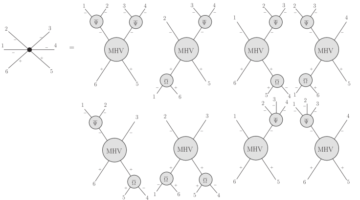
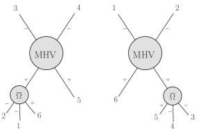
Figure 10: The contributions to the color-ordered 6 point $\overline{\text{MHV}}$ vertex, with helicity $(----++)$.

We checked, that the above expression reduces in the on-shell limit to the known expression:

$$\mathcal{A}(1^{-},2^{-},3^{-},4^{-},5^{+},6^{+})=g^{4}\left(\frac{p_{5}^{+}}{p_{6}^{+}}\right)^{2}\frac{\widetilde{v}_{65}^{4}}{\widetilde{v}_{16}\widetilde{v}_{65}\widetilde{v}_{54}\widetilde{v}_{43}\widetilde{v}_{32}\widetilde{v}_{21}}\,.$$ (95)

References

- [1] J. Collins, Foundations of perturbative QCD, vol. 32. Cambridge Univ. Press, 2011.
- [2] L. Lipatov, Gauge invariant effective action for high energy processes in QCD, Nucl. Phys. B 452 (oct, 1995) 369–397, [hep-ph/9502308].
- [3] F. Gelis, E. Iancu, J. Jalilian-Marian and R. Venugopalan, The Color Glass Condensate, Annu. Rev. Nucl. Part. Sci. 60 (nov, 2010) 463–489, [1002.0333].
- [4] A. Polyakov, Gauge fields as rings of glue, Nucl. Phys. B 164 (jan, 1980) 171–188.
- [5] I. O. Cherednikov, T. Mertens and F. F. Van der Veken, Wilson Lines in Quantum Field Theory, vol. 24. De Gruyter, sep, 2014, 10.1515/9783110309218.
- [6] R. Britto, F. Cachazo and B. Feng, New recursion relations for tree amplitudes of gluons, Nucl. Phys. B 715 (may, 2005) 499–522, [hep-th/0412308].
- [7] R. Britto, F. Cachazo, B. Feng and E. Witten, Direct Proof of the Tree-Level Scattering Amplitude Recursion Relation in Yang-Mills Theory, Phys. Rev. Lett. 94 (may, 2005) 181602, [hep-th/0501052].
- [8] K. Risager, A direct proof of the CSW rules, J. High Energy Phys. 2005 (dec, 2005) 003–003.
- [9] F. Cachazo, P. Svrcek and E. Witten, MHV Vertices And Tree Amplitudes In Gauge Theory, J. High Energy Phys. 2004 (sep, 2004) 006–006.
- [10] A. Gorsky and A. Rosly, From yang-mills lagrangian to MHV diagrams, Journal of High Energy Physics 2006 (jan, 2006) 101–101.
- [11] P. Mansfield, The lagrangian origin of MHV rules, J. High Energy Phys. 2006 (mar, 2006) 037–037.
- [12] J. H. Ettle and T. R. Morris, Structure of the MHV-rules lagrangian, J. High Energy Phys. 2006 (aug, 2006) 003–003.
- [13] S. Buchta and S. Weinzierl, The MHV lagrangian for a spontaneously broken gauge theory, Journal of High Energy Physics 2010 (Sep, 2010) .
- [14] T. R. Morris and Z. Xiao, The canonical transformation and massive CSW vertices for MHV-SQCD, Journal of High Energy Physics 2008 (dec, 2008) 028–028.
- [15] H. Feng and Y.-t. Huang, MHV lagrangian for n= 4 super yang-mills, Journal of High Energy Physics 2009 (Apr, 2009) 047–047.
- [16] C.-H. Fu, Generating MHV super-vertices in light-cone gauge, Journal of High Energy Physics 2010 (Apr, 2010) .
- [17] J. H. Ettle, C.-H. Fu, J. P. Fudger, P. R. Mansfield and T. R. Morris, S-matrix equivalence theorem evasion and dimensional regularisation with the canonical MHV lagrangian, J. High Energy Phys. 2007 (may, 2007) 011–011.
- [18] A. Brandhuber, B. Spence and G. Travaglini, Amplitudes in pure Yang-Mills and MHV Diagrams, J. High Energy Phys. 2007 (feb, 2007) 088–088.
- [19] A. Brandhuber, B. Spence, G. Travaglini and K. Zoubos, One-loop MHV rules and pure Yang-Mills, J. High Energy Phys. 2007 (jul, 2007) 002–002.
- [20] J. H. Ettle, T. R. Morris and Z. Xiao, The MHV QCD Lagrangian, J. High Energy Phys. 2008 (aug, 2008) 103–103.
- [21] H. Feng and Y.-T. Huang, MHV Lagrangian for N = 4 super Yang-Mills, J. High Energy Phys. 2009 (apr, 2009) 047–047.
- [22] R. Boels and C. Schwinn, Deriving CSW rules for massive scalar legs and pure Yang-Mills loops, Journal of High Energy Physics 2008 (Jul, 2008) 007–007.
- [23] H. Elvang, D. Z. Freedman and M. Kiermaier, Integrands for QCD rational terms and sym from massive CSW rules, Journal of High Energy Physics 2012 (Jun, 2012) .
- [24] A. Brandhuber, B. Spence and G. Travaglini, One-loop gauge theory amplitudes in super yang–mills from mhv vertices, Nuclear Physics B 706 (Jan, 2005) 150–180.
- [25] J. Bedford, A. Brandhuber, B. Spence and G. Travaglini, A twistor approach to one-loop amplitudes in supersymmetric Yang–Mills theory, Nuclear Physics B 706 (Jan, 2005) 100–126.
- [26] J. Bedford, A. Brandhuber, B. Spence and G. Travaglini, Non-supersymmetric loop amplitudes and MHV vertices, Nuclear Physics B 712 (Apr, 2005) 59–85.
- [27] P. Kotko and A. M. Stasto, Wilson lines in the MHV action, J. High Energy Phys. 2017 (2017) 47.
- [28] H. Kakkad, P. Kotko and A. Stasto, Exploring straight infinite Wilson lines in the self-dual and the MHV Lagrangians, Phys. Rev. D 102 (nov, 2020) 094026.
- [29] J. Scherk and J. H. Schwarz, Gravitation in the light cone gauge, Gen. Relativ. Gravit. 6 (1975) 537–550.
- [30] W. Bardeen, Self-dual Yang-Mills theory, integrability and multiparton amplitudes, Prog. Theor. Phys. Suppl. (1996) 1–8.
- [31] G. Chalmers and W. Siegel, Self-dual sector of QCD amplitudes, Phys. Rev. D 54 (dec, 1996) 7628–7633, [hep-th/9606061].
- [32] D. Cangemi, Self-dual Yang-Mills theory and one-loop maximally helicity violating multi-gluon amplitudes, Nucl. Phys. B 484 (jan, 1997) 521–537, [hep-th/9605208].
- [33] A. A. Rosly and K. G. Selivanov, On amplitudes in the self-dual sector of Yang-Mills theory, Phys. Lett. B 399 (1997) 135–140.
- [34] R. Monteiro and D. O’Connell, The kinematic algebra from the self-dual sector, J. High Energy Phys. 2011 (2011) 1–29, [arXiv:1105.2565v2].
- [35] L. Motyka and A. M. Staśto, Exact kinematics in the small-x evolution of the color dipole and gluon cascade, Phys. Rev. D 79 (apr, 2009) 085016, [0901.4949].
- [36] C. Cruz-Santiago, P. Kotko and A. M. Staśto, Recursion relations for multi-gluon off-shell amplitudes on the light-front and Wilson lines, Nucl. Phys. B 895 (2015) 132–160.
- [37] D. A. Kosower, Light-cone recurrence relations for QCD amplitudes, Nucl. Phys. B 335 (apr, 1990) 23–44.
- [38] L. J. Dixon, J. M. Henn, J. Plefka and T. Schuster, All tree-level amplitudes in massless QCD, J. High Energy Phys. 2011 (jan, 2011) 35, [1010.3991].
- [39] D. Maitre and P. Mastrolia, S@M, a Mathematica Implementation of the Spinor-Helicity Formalism, Comput. Phys. Commun. 179 (oct, 2007) 501–534, [0710.5559].