Selective Excitation of Subwavelength Atomic Clouds

Abstract

A dense cloud of atoms with randomly changing positions exhibits coherent and incoherent scattering. We show that an atomic cloud of subwavelength dimensions can be modeled as a single scatterer where both coherent and incoherent components of the scattered photons can be fully explained based on effective multipole moments. This model allows us to arrive at a relation between the coherent and incoherent components of scattering based on the conservation of energy. Furthermore, using superposition of four plane waves, we show that one can selectively excite different multipole moments and thus tailor the scattering of the atomic cloud to control the cooperative shift, resonance linewidth, and the radiation pattern. Our approach provides a new insight into the scattering phenomena in atomic ensembles and opens a pathway towards controlling scattering for applications such as generation and manipulation of single-photon states.

I Introduction

Since Dicke’s original work in 1954, the physics of collective effects and multiple scattering of light by a dense ensemble of atoms has attracted significant attention Dicke (1954); Lehmberg (1970); Friedberg et al. (1973); Gross and Haroche (1982); Guerin et al. (2017). In particular, remarkable phenomena such as Anderson localization Kramer and MacKinnon (1993); Skipetrov and Sokolov (2015), coherent backscattering Labeyrie et al. (1999), random lasing Baudouin et al. (2013), superradiance Dicke (1954); Scully and Svidzinsky (2009); Bienaimé et al. (2012); Araújo et al. (2016), subradiance Dicke (1954); Bienaimé et al. (2012); Guerin et al. (2016), and cooperative shift Roof et al. (2016) have been explored for cold ensembles of atoms. The physical origin of these phenomena can be understood by multiple scattering of light in a collection of atoms Sheng (2006). An ideal platform for observation of these cooperative effects is an array of cold atoms with subwavelength distances Jenkins and Ruostekoski (2012); Jenkins et al. (2016); Meir et al. (2014); Bettles et al. (2015, 2016a, 2016b); Facchinetti et al. (2016); Asenjo-Garcia et al. (2017); Shahmoon et al. (2017); Barredo et al. (2018); Wild et al. (2018); Facchinetti and Ruostekoski (2018); Guimond et al. (2019); Bekenstein et al. (2020); Rui et al. (2020); Alaee et al. (2020a, b); Ballantine and Ruostekoski (2020); Solntsev et al. (2020); Andreoli et al. (2021). However, arranging atoms in arbitrary subwavelength structures is highly demanding and cannot be achieved easily Rui et al. (2020). On the other hand, it has been demonstrated that a cloud of cold atoms can reach densities with atomic distances less than the resonant wavelength where a strong coherent dipole-dipole interaction couples the atoms Pellegrino et al. (2014); Jennewein et al. (2016). Therefore, the atoms interact with light collectively Pellegrino et al. (2014); Jennewein et al. (2016); Corman et al. (2017); Schilder et al. (2016, 2017); Browaeys and Lahaye (2020). Nonetheless, the linewidth and frequency of each collective mode depends strongly on the exact spatial arrangement of the atoms, which changes randomly even in a cold ensemble of atoms. As a consequence, the atomic cloud exhibits both coherent and incoherent scattering Schilder et al. (2016, 2017). Moreover, the random motion of the atoms seems to weaken the cooperative effects significantly and causes a subwavelength cloud of atoms to scatter fewer photons on average compared to a single atom, in contrast to Dicke’s work Schilder et al. (2020).

In this paper, we show that the cooperative shift and resonance linewidth of a subwavelength cloud of cold atoms can be controlled by structuring the excitation field. Structured light beams enable properties and applications in both classical and quantum optics Andrews (2011); Rubinsztein-Dunlop et al. (2016); Chekhova and Banzer (2021). In particular, structured light offers unique control of many phenomena including angstrom localization and detection of nanoparticles Roy et al. (2015); Neugebauer et al. (2016); Xi et al. (2016a); Bag et al. (2018), Kerker effects and directional scattering Xi et al. (2016b); Wei et al. (2017); Woźniak et al. (2015), counter-intuitive optical pulling and lateral forces Chen et al. (2011); Sukhov and Dogariu (2017), and nonlinear microscopy Bautista and Kauranen (2016), among other feats Andrews (2011); Das et al. (2015); Rubinsztein-Dunlop et al. (2016); Chekhova and Banzer (2021). However, the potential of structured light to manipulate cooperative effects remains unexplored.

We introduce a multipolar decomposition and demonstrate that both coherent and incoherent scattering of a subwavelength atomic cloud can be fully characterized by electric and magnetic multipole moments. Using conservation of energy and multipolar decomposition, we find analytical expressions that relate fluctuating and averaged electric and magnetic polarizabilities. Then, by employing superposition of four plane waves, we selectively excite the electric and magnetic multipole moments. As a result, we can control the cooperative shift and resonance linewidth of the atomic cloud by changing the relative phase between the plane waves.

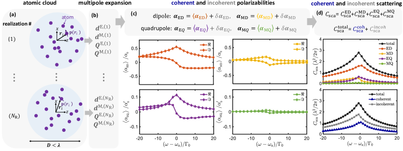
Figure 1: (a) Schematic drawing of a subwavelength atomic cloud composed of $N$ atoms at random positions for different realizations. $N_{\rm R}$ is the number of realizations. The diameter $D$ of the atomic cloud is smaller than the wavelength. (b) The induced electric and magnetic multipole moments of each realization obtained from multipole expansion of the induced current [using Eqs. (13) in the Appendix]. (c) Coherent electric and magnetic polarizabilities as a function of frequency detuning obtained from the induced multipole moments shown in (b). (d) Coherent and incoherent scattering cross sections and contribution of each multipole moment obtained from Eq. (4). The ensemble-averages are obtained from 10000 realizations of the atomic cloud with radius $R=0.2\lambda_{a}$ composed of $N=25$ atoms.

II Weak excitation limit

We consider a subwavelength cloud of atoms uniformly distributed in a sphere with radius R [see Fig. 1(a)]. The atomic cloud is assumed to be dense, i.e., $\rho/k^{3}>1$, where $\rho=N/V$ is the spatial density, $N$ is the number of atoms, and $V$ is the volume of the atomic cloud. We assume cold atoms without nonradiative losses and with a negligible Doppler effect compared to their radiative linewidth as in experimental realizations Pellegrino et al. (2014); Jennewein et al. (2016). The atomic cloud is investigated in the weak excitation limit such that the atomic transition is far below the saturation limit. Thus, each atom in the cloud is modeled by an isotropic electric polarizability given by $\alpha\left(\omega\right)=-(\alpha_{0}\Gamma_{0}/2)/\left(\omega-\omega_{a}+i\Gamma_{0}/2\right)$, where $\Gamma_{0}$ is the radiative linewidth, $\omega_{a}$ is the atomic transition angular frequency, and $\omega-\omega_{a}\ll\omega_{a}$ is the detuning of the illumination from the atomic resonance. $\alpha_{0}=6\pi/k^{3}$, where $k=\omega/c$ is the wavenumber of the illumination Lagendijk and Van Tiggelen (1996); De Vries et al. (1998); Lambropoulos and Petrosyan (2007); Alaee et al. (2017).

III Coherent and incoherent multipole expansion

We assume that the atoms in the subwavelength cloud have random spatial distributions. We consider many realizations for which the position of the atoms are changed with a uniform probability distribution [see Fig. 1(a)]. The atomic cloud is illuminated by plane waves and the total scattered field can be decomposed into two parts: $\mathbf{E}_{{\rm sca}}=\left\langle\mathbf{E}_{{\rm sca}}\right\rangle+\mathbf{\delta E}_{{\rm sca}}$, where $\left\langle\mathbf{E}_{{\rm sca}}\right\rangle$ and $\mathbf{\delta E}_{{\rm sca}}$ are the coherent (ensemble-averaged) and incoherent (fluctuating) fields, respectively Schilder et al. (2016, 2017, 2020). The induced polarization current density of the atomic cloud is given by $\mathbf{J}\left(\mathbf{r},\omega\right)=-i\omega\sum_{i=1}^{N}\mathbf{p}\left(\mathbf{r}_{i}\right)\delta\left(\mathbf{r}-\mathbf{r}_{i}\right)$ Tai (1994); Jackson (1999); Alaee et al. (2020a, b), where $\delta$ is the Dirac delta function and $\mathbf{p}\left(\mathbf{r}_{i}\right)$ is the induced electric dipole moment of the $i$th atom placed at $\mathbf{r}_{i}$ [see Fig. 1(a)]. Now by employing multipole decomposition of the current $\mathbf{J}\left(\mathbf{r},\omega\right)$ Alaee et al. (2018, 2019), we can calculate the induced effective multipole moments of the atomic cloud which can be decomposed into coherent and incoherent parts (see Appendix B for details):

$$d^{\rm E}_{\mu} = \left\langle d^{\rm E}_{\mu}\right\rangle+\delta d^{\rm E}_{\mu},\,\,\,\,\,\,\,\,\,\,d^{\rm M}_{\mu}=\left\langle d^{\rm M}_{\mu}\right\rangle+\delta d^{\rm M}_{\mu},$$

$$Q^{\rm E}_{\mu\nu} = \left\langle Q^{\rm E}_{\mu\nu}\right\rangle+\delta Q^{\rm E}_{\mu\nu},\,\,\,\,\,\,\,\,\,\,Q^{\rm M}_{\mu\nu}=\left\langle Q^{\rm M}_{\mu\nu}\right\rangle+\delta Q^{\rm M}_{\mu\nu},$$ (1)

where, $\mu,\nu\in{x,y,z}$. The quantities $d^{\rm E}_{\mu}$, $d^{\rm M}_{\mu}$, $Q^{\rm E}_{\mu\nu}$, and $Q^{\rm M}_{\mu\nu}$ are the effective electric dipole (ED), magnetic dipole (MD), electric quadrupole (EQ), and magnetic quadrupole (MQ) moments of the atomic cloud, respectively. The symbol $\left\langle\,\right\rangle$ represents an ensemble-average. Using the induced multipole moments, we obtain the electric and magnetic dipole and quadrupole polarizabilities

$$\bm{\alpha}_{i}=\left\langle\bm{\alpha}_{i}\right\rangle+\delta\bm{\alpha}_{i},\,\,\,\,\,i\in\left\{\mathrm{ED,MD,EQ,MQ}\right\},$$ (2)

where $\left\langle\bm{\alpha}_{i}\right\rangle$ and $\delta\bm{\alpha}_{i}$ are the coherent and incoherent polarizabilities, respectively.

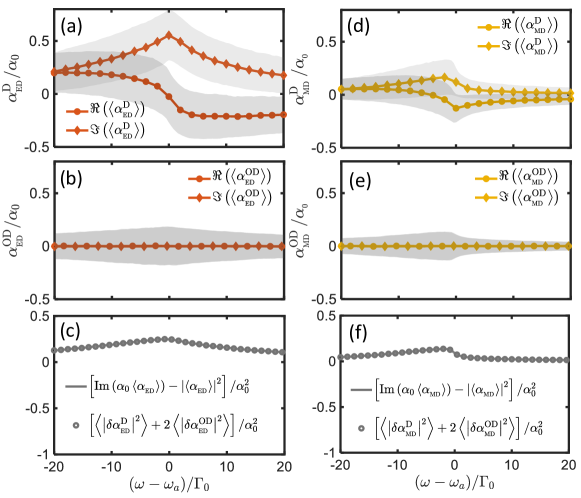
Figure 2: Coherent and incoherent electric and magnetic polarizabilities obtained from the induced multipole moments and defined as $\alpha_{i}^{j}=\left\langle\alpha_{i}^{j}\right\rangle+\delta\alpha_{i}^{j}$, where $i\in\left\{\mathrm{ED,MD}\right\},j\in\left\{\mathrm{D,OD}\right\}$. ED (MD) denotes the electric (magnetic) dipole and D (OD) represents diagonal (off-diagonal) components of the polarizability tensor (see Eq. 5). (a)-(b) Electric dipole polarizabilities as a function of frequency detuning. Note that $\left\langle\alpha_{\mathrm{{}_{ED}}}^{\mathrm{D}}\right\rangle\neq 0$ whereas $\left\langle\alpha_{{}_{\mathrm{ED}}}^{\mathrm{OD}}\right\rangle=0$. The thickness of the shaded lines show the fluctuating components of the polarizabilities. (c) Relation between coherent and incoherent polarizabilities obtained from the conservation of energy, see the left and right sides of Eq. (6). (d)-(f) Same as (a)-(c) for the magnetic dipole polarizability of the atomic cloud.

IV Single plane wave excitation

We consider a subwavelength atomic cloud composed of $N$ atoms as shown in Fig. 1 (a) and illuminated by an $x$-polarized plane wave $\mathbf{E_{\rm inc}}=E_{0}e^{ikz}\mathbf{e}_{x}$ propagating in the $z$ direction. The ensemble-averaged induced multipole moments are given by (see Appendix C for details)

$$\left\langle\mathbf{d}^{\mathrm{E}}\right\rangle = \varepsilon_{0}\left\langle\alpha_{{}_{\mathrm{ED}}}\right\rangle E_{0}\mathbf{e}_{x},\,\,\,\,\,\,\left\langle\mathbf{d}^{\mathrm{M}}\right\rangle=\left\langle\alpha_{{}_{\mathrm{MD}}}\right\rangle H_{0}\mathbf{e}_{y},$$

$$\left\langle\mathbf{Q}^{\mathrm{E}}\right\rangle = \frac{ik}{2}\varepsilon_{0}\left\langle\alpha_{{}_{\mathrm{EQ}}}\right\rangle E_{0}\left(\mathbf{e}_{x}\mathbf{e}_{z}+\mathbf{e}_{z}\mathbf{e}_{x}\right),$$

$$\left\langle\mathbf{Q}^{\mathrm{M}}\right\rangle = \frac{ik}{2}\left\langle\alpha_{{}_{\mathrm{MQ}}}\right\rangle H_{0}\left(\mathbf{e}_{y}\mathbf{e}_{z}+\mathbf{e}_{z}\mathbf{e}_{y}\right),$$ (3)

where, $\mathbf{Q}^{\mathrm{E}}$ and $\mathbf{Q}^{\mathrm{M}}$ are tensors of rank two, $\mathbf{e}_{\mu}\mathbf{e}_{\nu}$ is the unit dyad, $\mu,\nu\in{x,y,z}$, and $H_{0}$ is the amplitude of the magnetic field of the plane wave. Having the polarizabilities, we can calculate the coherent and total scattering cross sections by (see Appendix C)

$$C_{\mathrm{sca}}^{\mathrm{coh}} = \frac{3\lambda^{2}}{2\pi\alpha_{0}^{2}}\left(\left|\left\langle\alpha_{{}_{\mathrm{ED}}}\right\rangle\right|^{2}+\left|\left\langle\alpha_{{}_{\mathrm{MD}}}\right\rangle\right|^{2}\right)$$

$$+\frac{5\lambda^{2}}{2\pi{\alpha_{0}^{\prime}}^{2}}\left(\left|\left\langle\alpha_{{}_{\mathrm{EQ}}}\right\rangle\right|^{2}+\left|\left\langle\alpha_{{}_{\mathrm{MQ}}}\right\rangle\right|^{2}\right),$$

$$C_{\mathrm{sca}}^{\mathrm{\mathrm{total}}} = \frac{3\lambda^{2}}{2\pi\alpha_{0}^{2}}\mathrm{Im}\left(\left\langle\alpha_{{}_{\mathrm{ED}}}\right\rangle+\left\langle\alpha_{{}_{\mathrm{MD}}}\right\rangle\right)$$ (4)

$$+\frac{5\lambda^{2}}{2\pi{\alpha_{0}^{\prime}}^{2}}\mathrm{Im}\left(\left\langle\alpha_{{}_{\mathrm{EQ}}}\right\rangle+\left\langle\alpha_{{}_{\mathrm{MQ}}}\right\rangle\right),$$

where $\alpha_{0}=6\pi/k^{3}$ ($\alpha_{0}^{\prime}=120\pi/k^{5}$) is related to the radiation loss of a dipole (quadrupole) moment. Equation (4), which is the first main result of this paper, allows us to calculate the coherent and incoherent scattering cross sections of the atomic ensemble. Note that the incoherent scattering cross section is given by $C_{\mathrm{sca}}^{\mathrm{incoh}}=C_{\mathrm{sca}}^{\mathrm{total}}-C_{\mathrm{sca}}^{\mathrm{coh}}$. We consider now a spherical subwavelength atomic cloud with radius $R=0.2\lambda_{a}$ composed of 25 atoms which can be fully characterized by dipole and quadrupole moments. Figure 1 (c) shows that the atomic cloud exhibits strong electric and magnetic responses. Figure 1(d) shows the coherent, incoherent and total scattering cross sections (normalized to $\lambda^{2}/2\pi$) calculated from Eq. (4), and the contribution of different multipole moments as a function of frequency detuning. It can be seen that the maximum total scattering cross section of the ensemble is approximately equal to the scattering of a single atom, even though the atomic cloud consists of 25 atoms Schilder et al. (2020). Furthermore, the maximum cross section of coherent scattering is much smaller than that of a single atom Schilder et al. (2016, 2017, 2020).

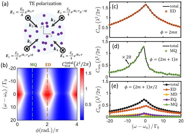
Figure 3: Selective excitation of ED and MQ moments using four TE polarized plane waves. (a) Schematic drawing of a subwavelength atomic cloud when illuminated by four plane waves. $\phi$ is the relative phase between the plane waves. (b) Normalized ensemble-averaged scattering cross section of the atomic cloud as a function of frequency detuning and the relative phase $\phi$. The red and green dashed lines depict selective excitation of pure ED and MQ moments, respectively. (c)-(e) Normalized ensemble-averaged total scattering cross sections as a function of frequency detuning for different phase (c) $\phi=2m\pi$, (d) $\phi=(2m+1)\pi$, and (e) $\phi=(2m+1)\pi/2$. The ensemble-averages are obtained from 10000 realizations of the atomic cloud.

In order to establish the relation between the coherent and incoherent polarizabilities, we focus only on the dipolar response of the atomic cloud for simplicity. The supplementary material provides the relations for other multipole moments. Note that the ensemble-averaged polarizability of a spherical atomic cloud is isotropic, i.e. $\left\langle\bm{\alpha}_{i}\right\rangle=\left\langle\alpha_{i}\right\rangle\mathbf{I}$, where $\mathbf{I}$ is the identity matrix. Therefore, all the diagonal matrix elements of the induced electric dipole polarizability are identical and are represented by $\alpha_{{}_{\mathrm{ED}}}^{\mathrm{D}}$. All the off-diagonal elements, $\alpha_{{}_{\mathrm{ED}}}^{\mathrm{OD}}$, are also identical. Therefore, the induced electric dipole polarizability can be written as

$$\bm{\alpha}_{{}_{\mathrm{ED}}}=\left(\left\langle\alpha_{{}_{\mathrm{ED}}}\right\rangle+\delta\alpha_{{}_{\mathrm{ED}}}^{\mathrm{D}}\right)\mathbf{I}+\delta\alpha_{{}_{\mathrm{ED}}}^{\mathrm{OD}}\left(\mathbf{J}-\mathbf{I}\right),$$ (5)

where $\mathbf{J}$ is the all-ones matrix. Note also that $\left\langle\bm{\alpha}_{{}_{\mathrm{ED}}}\right\rangle=\left\langle\alpha_{{}_{\mathrm{ED}}}\right\rangle\mathbf{I}\,\,$ and $\left\langle\alpha_{{}_{\mathrm{ED}}}^{\mathrm{OD}}\right\rangle=0$. Using conservation of energy, we get (see Appendix B)

$$\mathrm{Im}\left(\alpha_{0}\left\langle\alpha_{{}_{\mathrm{ED}}}\right\rangle\right)-\left|\left\langle\alpha_{{}_{\mathrm{ED}}}\right\rangle\right|^{2} = \left\langle\left|\delta\alpha_{{}_{\mathrm{ED}}}^{\mathrm{D}}\right|^{2}\right\rangle+2\left\langle\left|\delta\alpha_{{}_{\mathrm{ED}}}^{\mathrm{OD}}\right|^{2}\right\rangle.$$ (6)

Equation (6) is the second main result of this paper; it shows how the fluctuations of the polarizabilities can be obtained from the ensemble-averaged values (see Appendix B) for the details of the derivation and similar expressions for MD, EQ, MQ polarizability tensors). In Fig. 2(a)-(b), we plot the coherent and incoherent electric dipole polarizabilities retrieved from multipolar decomposition. In contrast to the off-diagonal terms, the diagonal term exhibits a non-zero ensemble-averaged polarizabiltiy. Note that the components of the electric dipole moment tensor satisfy Eq. (6) [see Fig. 2(c)]. Using the duality of the electric and magnetic fields in Maxwell’s equations and conservation of energy, we can obtain a similar relation for the components of the magnetic polarizability tensor (i.e., replacing MD with ED in Eq. (6), see Appendix B). Figure 2(d)-(e) shows the coherent and incoherent components of the magnetic polarizabilities. The magnetic response is smaller than the electric one. The induced multipole moments exhibit asymmetry in their resonance lineshape which explains the non-Lorentzian lineshape of the scattering cross sections in Fig. 1(d).

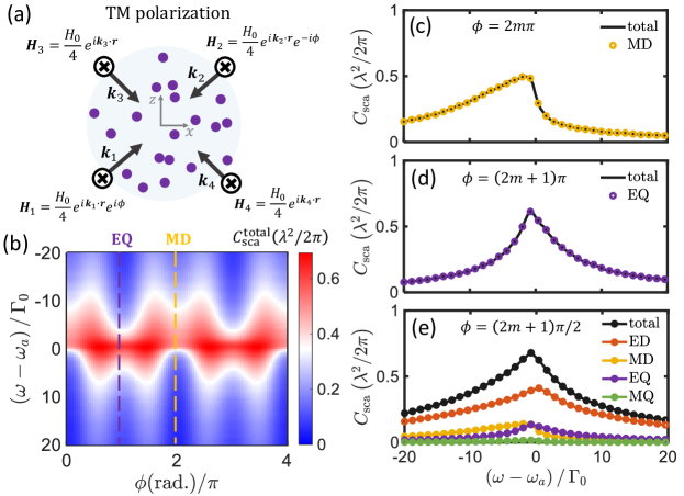
Figure 4: Selective excitation of MD and EQ moments using four TM polarized plane waves. (a) Schematic drawing of a subwavelength atomic cloud when illuminated by four plane waves. $\phi$ is the relative phase between the plane waves. (b) Normalized ensemble-averaged scattering cross section of the atomic cloud as a function of frequency detuning and the relative phase between input plane waves. The orange and purple dashed lines depict selective excitation of pure MD and EQ moments, respectively. (c)-(e) Normalized ensemble-averaged scattering cross sections as a function of frequency detuning for different phase (c) $\phi=2m\pi$, (d) $\phi=(2m+1)\pi$, and (e) $\phi=(2m+1)\phi/2$. The ensemble-averages are obtained from 10000 realizations of the atomic cloud.

V Selective excitation of electric dipole or magnetic quadrupole moment

Although the constituent atoms have only electric dipole transitions, the entire atomic cloud can support higher order electric and magnetic multipole moments [see Fig. 1 (d)]. Here, we show that it is possible to selectively excite a particular multipole moment by tailoring the excitation field. To this end, we consider an excitation by four plane waves with TE polarization, i.e., $\mathbf{E}_{\mathrm{inc}}=E_{0}/4\sum_{n=1}^{4}e^{i\left(\mathbf{k}_{n}\cdot\mathbf{r}+\phi_{n}\right)}\mathbf{e}_{y},$ where $\mathbf{k}_{1}=-\mathbf{k}_{2}=k\left(\mathrm{sin}\psi\mathbf{e}_{x}+\mathrm{cos}\psi\mathbf{e}_{z}\right)$, $\mathbf{k}_{3}=-\mathbf{k}_{4}=k\left(\mathrm{sin}\psi\mathbf{e}_{x}-\mathrm{cos}\psi\mathbf{e}_{z}\right),$ $\phi_{1}=-\phi_{2}\equiv\phi$, $\phi_{3}=\phi_{4}=0$ and $\psi=\pi/4$ [see Fig. 3 (a)]. Hence, the ensemble-averaged induced multipole moments are given by (see Appendix D)

$$\left\langle\mathbf{d}^{\mathrm{E}}\right\rangle = \varepsilon_{0}\left\langle\alpha_{{}_{\mathrm{ED}}}\right\rangle E_{0}\mathrm{cos}^{2}\frac{\phi}{2}\mathbf{e}_{y},$$

$$\left\langle\mathbf{d}^{\mathrm{M}}\right\rangle = -i\left\langle\alpha_{{}_{\mathrm{MD}}}\right\rangle H_{0}\mathrm{sin}\frac{\phi}{2}\mathrm{cos}\frac{\phi}{2}\left(\mathbf{e}_{x}-\mathbf{e}_{z}\right)/\sqrt{2},$$

$$\left\langle\mathbf{Q}^{\mathrm{E}}\right\rangle = -\varepsilon_{0}\frac{k}{2}\left\langle\alpha_{{}_{\mathrm{EQ}}}\right\rangle E_{0}\mathrm{sin}\frac{\phi}{2}\mathrm{cos}\frac{\phi}{2}\left\{\mathbf{e}_{y}\mathbf{e}_{x}+\mathbf{e}_{x}\mathbf{e}_{y}\right.$$

$$+\left.\mathbf{e}_{y}\mathbf{e}_{z}+\mathbf{e}_{z}\mathbf{e}_{y}\right\}/\sqrt{2},$$

$$\left\langle\mathbf{Q}^{\mathrm{M}}\right\rangle = -\frac{ik}{2}\left\langle\alpha_{{}_{\mathrm{MQ}}}\right\rangle H_{0}\mathrm{sin}^{2}\frac{\phi}{2}\left(\mathbf{e}_{z}\mathbf{e}_{z}-\mathbf{e}_{x}\mathbf{e}_{x}\right).$$ (7)

Equation (7) clearly shows that by changing the relative phase $\phi$, one can control which multipole moment to be excited. Consequently, the scattering cross sections are given by (see Appendix D)

$$C_{\mathrm{sca}}^{\mathrm{coh}} = \frac{3\lambda^{2}}{2\pi\alpha_{0}^{2}}\left(\left|\left\langle\alpha_{{}_{\mathrm{ED}}}\right\rangle\right|^{2}\mathrm{cos}^{4}\frac{\phi}{2}+\left|\left\langle\alpha_{{}_{\mathrm{MD}}}\right\rangle\right|^{2}\mathrm{sin}^{2}\frac{\phi}{2}\mathrm{cos}^{2}\frac{\phi}{2}\right)$$

$$+\frac{5\lambda^{2}}{2\pi\alpha_{0}^{\prime 2}}\left(\left|\left\langle\alpha_{{}_{\mathrm{EQ}}}\right\rangle\right|^{2}\mathrm{sin}^{2}\frac{\phi}{2}\mathrm{cos}^{2}\frac{\phi}{2}+\left|\left\langle\alpha_{{}_{\mathrm{MQ}}}\right\rangle\right|^{2}\mathrm{sin}^{4}\frac{\phi}{2}\right),$$

$$C_{\mathrm{sca}}^{\mathrm{total}} = \frac{3\lambda^{2}}{2\pi\alpha_{0}}\mathrm{Im}\left(\left\langle\alpha_{{}_{\mathrm{ED}}}\right\rangle\mathrm{cos}^{4}\frac{\phi}{2}+\left\langle\alpha_{{}_{\mathrm{MD}}}\right\rangle\mathrm{sin}^{2}\frac{\phi}{2}\mathrm{cos}^{2}\frac{\phi}{2}\right)$$

$$+\frac{5\lambda^{2}}{2\pi\alpha_{0}^{\prime}}\mathrm{Im}\left(\left\langle\alpha_{{}_{\mathrm{EQ}}}\right\rangle\mathrm{sin}^{2}\frac{\phi}{2}\mathrm{cos}^{2}\frac{\phi}{2}+\left\langle\alpha_{{}_{\mathrm{MQ}}}\right\rangle\mathrm{sin}^{4}\frac{\phi}{2}\right).$$

Equations (7) and (V) are the third main result of this paper which show that the induced dipole moments and the scattering cross sections can be controlled by a simple four-beam configuration and the relative phase $\phi$ between the plane waves. Figure 3(b) plots the scattering cross section as a function of the relative phase and the frequency detuning. Interestingly, as can be seen from Fig. 3(c) and (d), the cooperative resonance linewidth can also be tuned by varying the phase $\phi$ due to selective exciation of different multipole moments.

We note three different scenarios based on the relative phase $\phi$:

(i) At $\phi=2m\pi$, where $m$ is a non-negative integer, only the electric dipole moment of the atomic cloud is excited [see Eq. (7) and Fig. 3(c)]. In this case, the atomic cloud exhibits an omnidirectional radiation pattern.

(ii) At $\phi=(2m+1)\pi$, according to Eq. (7), the atomic cloud exhibits only a magnetic quadrupole moment as shown in Fig. 3(d) and scatters light with a quadrupolar pattern.

(iii) At $2m\pi<\phi<\left(2m+1\right)\pi$, all multipoles can be excited, see for example Fig. 3(e) for $\phi=(2m+1)\pi/2$. Thus, one can selectively excite the electric dipole or magnetic quadrupole moment of the atomic cloud by just controlling the relative phase of the plane waves with TE polarizations and achieve arbitrary radiation patterns.

VI Selective excitation of magnetic dipole or electric quadrupole moment

To selectively excite magnetic dipole or electric quadrupole, we employ superposition of four plane waves with TM polarization: $\mathbf{H}_{\mathrm{inc}}=H_{0}/4\sum_{n=1}^{4}e^{i\left(\mathbf{k}_{n}\cdot\mathbf{r}+\phi_{n}\right)}\mathbf{e}_{y},$ where $\mathbf{k}_{n}$ and $\phi_{n}$ are defined similar to the TE polarization, see the previous section and Fig. 4(a). The coherent and total scattering cross sections are thus given by (see Appendix D)

$$C_{\mathrm{sca}}^{\mathrm{coh}} = \frac{3\lambda^{2}}{2\pi\alpha_{0}^{2}}\left(\left|\left\langle\alpha_{{}_{\mathrm{ED}}}\right\rangle\right|^{2}\mathrm{sin}^{2}\frac{\phi}{2}\mathrm{cos}^{2}\frac{\phi}{2}+\left|\left\langle\alpha_{{}_{\mathrm{MD}}}\right\rangle\right|^{2}\mathrm{cos}^{4}\frac{\phi}{2}\right)$$

$$+\frac{5\lambda^{2}}{2\pi\alpha_{0}^{\prime 2}}\left(\left|\left\langle\alpha_{{}_{\mathrm{EQ}}}\right\rangle\right|^{2}\mathrm{sin}^{4}\frac{\phi}{2}+\left|\left\langle\alpha_{{}_{\mathrm{MQ}}}\right\rangle\right|^{2}\mathrm{sin}^{2}\frac{\phi}{2}\mathrm{cos}^{2}\frac{\phi}{2}\right),$$

$$C_{\mathrm{sca}}^{\mathrm{total}} = \frac{3\lambda^{2}}{2\pi\alpha_{0}}\mathrm{Im}\left(\left\langle\alpha_{{}_{\mathrm{ED}}}\right\rangle\mathrm{sin}^{2}\frac{\phi}{2}\mathrm{cos}^{2}\frac{\phi}{2}+\left\langle\alpha_{{}_{\mathrm{MD}}}\right\rangle\mathrm{cos}^{4}\frac{\phi}{2}\right)$$

$$+\frac{5\lambda^{2}}{2\pi\alpha_{0}^{\prime}}\mathrm{Im}\left(\left\langle\alpha_{{}_{\mathrm{EQ}}}\right\rangle\mathrm{sin}^{4}\frac{\phi}{2}+\left\langle\alpha_{{}_{\mathrm{MQ}}}\right\rangle\mathrm{sin}^{2}\frac{\phi}{2}\mathrm{cos}^{2}\frac{\phi}{2}\right).$$

Figure 4(b) plots the total scattering cross section as a function of the relative phase $\phi$ and the frequency detuning. As shown in Fig. 4(c) and 4(d), by varying the phase $\phi$, one can excite different multipole moments and thus control the cooperative shift and resonance linewidth. In particular, the MD and EQ moments can be selectively excited by the TM polarized plane waves. As a consequence, the atomic cloud will scatter light in a selective direction depending on the relative phase between the plane waves.

Arrays of cold atoms with subwavelength spacing scatter light coherently and thus have been modeled by effective electric and magnetic multipole moments Alaee et al. (2020a, b); Ballantine and Ruostekoski (2020). In contrast, an atomic cloud composed of randomly distributed atoms exhibits not only coherent, but also incoherent scattering due to the motion of the atoms Schilder et al. (2016, 2017, 2020). In this paper, we showed that the multipolar decomposition can model not only the coherent, but also the incoherent response of the atomic cloud accurately. We also demonstrated that the ensemble-averaged polarizabilities are adequate to model the response of the atomic cloud. Furthermore, using superposition of plane waves, we showed that one can selectively excite the induced electric and magnetic multipole moments and thus manipulate the resonant linewidth and cooperative shift of the ensemble, as well as its radiation pattern. Our study paves the way towards controlling cooperative effects in atomic systems through structured light Andrews (2011); Rubinsztein-Dunlop et al. (2016). Our approach to control the cooperative effects is not restricted to subwavelength cold atomic clouds and can be realized both experimentally and theoretically in different systems of interacting quantum emitters including ultracold quantum metasurfaces Rui et al. (2020), nanoscale atomic vapor layer Peyrot et al. (2018), two-dimensional semiconductors heterostructures Scuri et al. (2020), and atomic arrays in waveguides and cavities Sheremet et al. (2021).

Acknowledgments.— R. A. is grateful to Vahid Sandoghdar, Boris Braverman, and Zeinab Mokhtari for helpful discussions and acknowledges the support of the Alexander von Humboldt Foundation through the Feodor Lynen (Return) Research Fellowship. R.A., A.S., and R.W.B. acknowledge support through the Natural Sciences and Engineering Research Council of Canada, the Canada Research Chairs program, and the Canada First Research Excellence Fund.

VII Appendices

Appendix A Atomic polarizability and coupled-dipole equations

Let us consider an atomic cloud composed of neutral atoms with only electric dipole transition moments and illuminated by a plane wave [see Fig. 1 (a)]. The atoms confined in a volume smaller than the wavelength of the resonant light, i.e., $D<\lambda$. We consider the weak-excitation limit where the atomic response is isotropic and linear. The electric polarizability of each atom amounts to $\alpha\left(\omega\right)=-\left(\alpha_{0}\Gamma_{0}/2\right)/\left[\omega-\omega_{a}+i\left(\Gamma_{0}+\Gamma_{\mathrm{nr}}\right)/2\right]$, where $\Gamma_{0}$ is the radiative linewidth of the atomic transition at frequency $\omega_{a}$, and $\omega-\omega_{a}\ll\omega_{a}$ represents the frequency detuning between the illumination and the atomic resonance, $\alpha_{0}=6\pi/k^{3}$ and $k$ is the wavenumber Lagendijk and Van Tiggelen (1996); De Vries et al. (1998). We assume elastic scattering events and therefore the non-radiative decay rate is zero, i.e., $\Gamma_{\mathrm{nr}}=0$. The induced dipole moment of the $i$th atom $\mathbf{p}\left(\mathbf{r}_{i}\right)=\epsilon_{0}\alpha\mathbf{E}_{\mathrm{loc}}\left(\mathbf{r}_{i}\right)$ can be obtained by using the coupled-dipole equations Lagendijk and Van Tiggelen (1996); De Vries et al. (1998); Alaee et al. (2017)

$$\mathbf{p}\left(\mathbf{r}_{i}\right) = \epsilon_{0}\alpha\left[\mathbf{E}_{\mathrm{inc}}\left(\mathbf{r}_{i}\right)+\sum_{i\neq j}\mathbf{G}\left(\mathbf{r}_{i},\mathbf{r}_{j}\right)\mathbf{p}\left(\mathbf{r}_{j}\right)\right],$$ (10)

where $\mathbf{E}_{\mathrm{inc}}\left(\mathbf{r}_{i}\right)$ is the incident field at the position $\mathbf{r}_{i}$ of the atom, and $\alpha$ is the atomic polarizability. The total field at the position of the $i$th atom $\mathbf{E}_{\mathrm{loc}}\left(\mathbf{r}_{i}\right)$ is the sum of the incident field and the scattered field from the other atoms. The electric dipole at position $\mathbf{r}_{j}$ radiates an electromagnetic field which when measured at $\mathbf{r}_{i}$ can be calculated from $\mathbf{G}\left(\mathbf{r}_{i},\mathbf{r}_{j}\right)\mathbf{p}\left(\mathbf{r}_{j}\right)$, where $\mathbf{G}\left(\mathbf{r}_{i},\mathbf{r}_{j}\right)$ is Green’s tensor given by Tai (1994); Jackson (1999)

$$\text{$\mathbf{G}\left(\mathbf{r}_{i},\mathbf{r}_{j}\right)$=$\frac{3}{2\alpha_{0}\epsilon_{0}}e^{i\zeta}\left[g_{1}\left(\zeta\right)\bar{\bar{{\bf I}}}+g_{2}\left(\zeta\right)\mathbf{\mathbf{n}n}\right]$},$$ (11)

where

$$g_{1}\left(\zeta\right) = \left(\frac{1}{\zeta}-\frac{1}{\zeta^{3}}+\frac{i}{\zeta^{2}}\right),\,\,\,\,\,\,\,\,\,$$

$$g_{2}\left(\zeta\right) = \left(-\frac{1}{\zeta}+\frac{3}{\zeta^{3}}-\frac{3i}{\zeta^{2}}\right),$$ (12)

$\bar{\bar{{\bf I}}}$ is the identity dyadic, $\mathbf{n}=\frac{\mathbf{r}_{i}-\mathbf{r}_{j}}{\left|\mathbf{r}_{i}-\mathbf{r}_{j}\right|}$, and $\zeta=\left|k\left(\mathbf{r}_{i}-\mathbf{r}_{j}\right)\right|$ Alaee et al. (2020a, b). Having the induced dipole moment of each atom, we can define the induced displacement current $\mathbf{J}\left(\mathbf{r},\omega\right)=-i\omega\sum_{i=1}^{N}\mathbf{p}\left(\mathbf{r}_{i}\right)\delta\left(\mathbf{r}-\mathbf{r}_{i}\right)$, where $\delta$ is the Dirac delta function, and $\mathbf{p}\left(\mathbf{r}_{i}\right)$ is the induced electric dipole moment of the $i$th atom at $\mathbf{r}=\mathbf{r}_{i}$ [see Fig. 1 (a)]. Here, we assumed $e^{-i\omega t}$ as a time harmonic variation.

Appendix B Multipole expansion and cross sections

B.1 Coherent and incoherent multipole moments

In this subsection, we present expressions for the effective induced electric and magnetic moments in Cartesian coordinates Alaee et al. (2020a). Using the multipole expansion of the induced current $\mathbf{J}\left(\mathbf{r},\omega\right)$, the induced effective multipole moments of the atomic cloud (at the center $\mathbf{r}=0$) can be calculated Alaee et al. (2018, 2019):

$$d^{\rm E}_{\mu} = -\frac{1}{i\omega}\left\{\int d^{3}\mathbf{r}J_{\mu}j_{0}\left(kr\right)+\frac{k^{2}}{2}\int d^{3}\mathbf{r}\left[3\left(\mathbf{r}\cdot\mathbf{J}\right)r_{\mu}-r^{2}J_{\mu}\right]\frac{j_{2}\left(kr\right)}{\left(kr\right)^{2}}\right\},$$

$$d^{\rm M}_{\mu} = \frac{3}{2}\int d^{3}\mathbf{r}\left(\mathbf{r}\times\mathbf{J}\right)_{\mu}\frac{j_{1}\left(kr\right)}{kr},$$

$$Q^{\rm E}_{\mu\nu} = -\frac{3}{i\omega}\left\{\int d^{3}\mathbf{r}\left[3\left(r_{\nu}J_{\mu}+r_{\mu}J_{\nu}\right)-2\left(\mathbf{r}\cdot\mathbf{J}\right)\delta_{\mu\nu}\right]\frac{j_{1}\left(kr\right)}{kr}\right.$$

$$\left.+2k^{2}\int d^{3}\mathbf{r}\left[5r_{\mu}r_{\nu}\left(\mathbf{r}\cdot\mathbf{J}\right)-\left(r_{\mu}J_{\nu}+r_{\nu}J_{\mu}\right)r^{2}-r^{2}\left(\mathbf{r}\cdot\mathbf{J}\right)\delta_{\mu\nu}\right]\frac{j_{3}\left(kr\right)}{\left(kr\right)^{3}}\right\},$$

$$Q^{\rm M}_{\mu\nu} = 15\int d^{3}\mathbf{r}\left\{r_{\mu}\left(\mathbf{r}\times\mathbf{J}\right)_{\nu}+r_{\nu}\left(\mathbf{r}\times\mathbf{J}\right)_{\mu}\right\}\frac{j_{2}\left(kr\right)}{\left(kr\right)^{2}},$$ (13)

where, $\mu,\nu\in{x,y,z}$. The quantities $d^{\rm E}_{\mu}$, $d^{\rm M}_{\mu}$, $Q^{\rm E}_{\mu\nu}$, and $Q^{\rm M}_{\mu\nu}$ are the electric dipole (ED), magnetic dipole (MD), electric quadrupole (EQ), and magnetic quadrupole (MQ) multipole moments, respectively. $j_{n}$ are the spherical Bessel functions. Note that $\mathbf{Q}^{\mathrm{E}}=\sum_{\mu,\nu}Q^{\rm E}_{\mu\nu}\mathbf{e}_{\mu}\mathbf{e}_{\nu}$ and $\mathbf{Q}^{\mathrm{M}}=\sum_{\mu,\nu}Q^{\rm M}_{\mu\nu}\mathbf{e}_{\mu}\mathbf{e}_{\nu}$ are tensors of rank two and $\mathbf{e}_{\mu}\mathbf{e}_{\nu}$ is unit dyad. We consider $N_{\rm R}$ realizations for which the positions of the atoms are changed with a uniform probability distribution in a spherical volume. Then, the induced multipole moments of the atomic cloud can be decomposed into coherent (ensemble-averaged) and incoherent (fluctuating) parts:

$$d^{\rm E}_{\mu} = \left\langle d^{\rm E}_{\mu}\right\rangle+\delta d^{\rm E}_{\mu},\,\,\,\,\,\,\,\,\,\,d^{\rm M}_{\mu}=\left\langle d^{\rm M}_{\mu}\right\rangle+\delta d^{\rm M}_{i},$$ (14)

$$Q^{\rm E}_{\mu\nu} = \left\langle Q^{\rm E}_{\mu\nu}\right\rangle+\delta Q^{\rm E}_{\mu\nu},\,\,\,\,\,\,\,\,\,\,Q^{\rm M}_{\mu\nu}=\left\langle Q^{\rm M}_{\mu\nu}\right\rangle+\delta Q^{\rm M}_{\mu\nu},$$

where $\mu,\nu=x,y,z$. The symbols $\left\langle\cdot\right\rangle$ represent the ensemble-averaged multipole moments. Note that the incoherent multipole moments are related to the quasi-isotropic speckle originating from the random positions of the atoms in the spherical cloud.

B.2 Coherent and incoherent cross sections

In this subsection, we derive coherent and incoherent scattering and extinction cross sections using the induced electric and magnetic multipole moments in Eqs. (13)-(14). The total scattering cross section can be decomposed into coherent and incoherent parts, i.e., $C_{\mathrm{sca}}^{\mathrm{total}}=C_{\mathrm{sca}}^{\mathrm{coh}}+C_{\mathrm{sca}}^{\mathrm{incoh}}$ which are and given by Alaee et al. (2018, 2019)

$$C_{\mathrm{sca}}^{\mathrm{coh}} = \frac{k^{4}}{6\pi\varepsilon_{0}^{2}E_{0}^{2}}\sum_{\mu}\left(\left|\left\langle d_{\mu}^{\mathrm{E}}\right\rangle\right|^{2}+\left|\left\langle\frac{d_{\mu}^{\mathrm{M}}}{c}\right\rangle\right|^{2}\right)$$

$$+\frac{k^{6}}{720\pi\varepsilon_{0}^{2}E_{0}^{2}}\sum_{\mu,\nu}\left(\left|\left\langle Q_{\mu\nu}^{\mathrm{E}}\right\rangle\right|^{2}+\left|\left\langle\frac{Q_{\mu\nu}^{\mathrm{M}}}{c}\right\rangle\right|^{2}\right),$$

$$C_{\mathrm{sca}}^{\mathrm{incoh}} = \frac{k^{4}}{6\pi\varepsilon_{0}^{2}E_{0}^{2}}\sum_{\mu}\left(\left\langle\left|\delta d_{\mu}^{\mathrm{E}}\right|^{2}\right\rangle+\left\langle\left|\frac{\delta d_{\mu}^{\mathrm{M}}}{c}\right|^{2}\right\rangle\right)$$

$$+\frac{k^{6}}{720\pi\varepsilon_{0}^{2}E_{0}^{2}}\sum_{\mu,\nu}\left(\left\langle\left|\delta Q_{\mu\nu}^{\mathrm{E}}\right|^{2}\right\rangle+\left\langle\left|\frac{\delta Q_{\mu\nu}^{\mathrm{M}}}{c}\right|^{2}\right\rangle\right),$$

and the extinction cross section of the cloud is given by Alaee et al. (2018, 2019)

$$C_{\mathrm{ext}} = \frac{k}{\varepsilon_{0}E_{0}^{2}}\mathrm{Im}\left[\sum_{\mu}\left(\left\langle d_{\mu}^{\mathrm{E}}\right\rangle E_{\mu}^{*}+\left\langle\frac{d_{\mu}^{\mathrm{M}}}{c}\right\rangle Z_{0}H_{\mu}^{*}\right)\right]$$

$$+\frac{k}{12\varepsilon_{0}E_{0}^{2}}\mathrm{Im}\left[\sum_{\mu,\nu}\left\langle Q_{\mu\nu}^{\mathrm{E}}\right\rangle\left(\frac{\partial E_{\nu}^{*}}{\partial r_{\mu}}+\frac{\partial E_{\mu}^{*}}{\partial r_{\nu}}\right)\right]$$

$$+\frac{k}{12\varepsilon_{0}E_{0}^{2}}\mathrm{Im}\left[\sum_{\mu,\nu}\left\langle\frac{Q_{\mu\nu}^{\mathrm{M}}}{c}\right\rangle Z_{0}\left(\frac{\partial H_{\nu}^{*}}{\partial r_{\mu}}+\frac{\partial H_{\mu}^{*}}{\partial r_{\nu}}\right)\right],$$

where $Z_{0}$ is the impedance of free space, $c$ is the speed of light in free space, and $\mathbf{r}=\sum_{\mu}r_{\mu}\mathbf{e}_{\mu}=x\mathbf{e}_{x}+y\mathbf{e}_{y}+z\mathbf{e}_{z}$. Note that in Eq. (B.2) and also in the remainder of the supplementary material, $\mathbf{E}$ and $\mathbf{H}$ show the incident fields, i.e. we omit the subscript ”inc” for simplifying the notation.

B.3 Conservation of energy: coherent and incoherent cross sections

According to the conservation of energy, the extinction cross section is equal to the sum of the coherent and incoherent scattering cross sections, i.e., $C_{\mathrm{ext}}=C_{\mathrm{sca}}^{\mathrm{total}}=C_{\mathrm{sca}}^{\mathrm{coh}}+C_{\mathrm{sca}}^{\mathrm{incoh}}$. Therefore, from Eqs. (B.2)-(B.2), we obtain the following relations between the coherent and incoherent multipole moments:

$$\sum_{\mu}\left\langle\left|d_{\mu}^{\mathrm{E}}\right|^{2}\right\rangle = \sum_{\mu}\left[\left|\left\langle d_{\mu}^{\mathrm{E}}\right\rangle\right|^{2}+\left\langle\left|\delta d_{\mu}^{\mathrm{E}}\right|^{2}\right\rangle\right]$$

$$= \varepsilon_{0}\alpha_{0}\sum_{\mu}\mathrm{Im}\left[\left\langle d_{\mu}^{\mathrm{E}}\right\rangle E_{\mu}^{*}\right],$$

$$\sum_{\mu}\left\langle\left|d_{\mu}^{\mathrm{M}}\right|^{2}\right\rangle = \sum_{\mu}\left[\left|\left\langle d_{\mu}^{\mathrm{M}}\right\rangle\right|^{2}+\left\langle\left|\delta d_{\mu}^{\mathrm{M}}\right|^{2}\right\rangle\right]$$

$$= \alpha_{0}\sum_{\mu}\mathrm{Im}\left[\left\langle d_{\mu}^{\mathrm{M}}\right\rangle H_{\mu}^{*}\right],$$

$$\sum_{\mu,\nu}\left\langle\left|Q_{\mu\nu}^{\mathrm{E}}\right|^{2}\right\rangle = \sum_{\mu,\nu}\left[\left|\left\langle Q_{\mu\nu}^{\mathrm{E}}\right\rangle\right|^{2}+\left\langle\left|\delta Q_{\mu\nu}^{\mathrm{E}}\right|^{2}\right\rangle\right]$$

$$= \frac{1}{2}\varepsilon_{0}\alpha_{0}^{\prime}\sum_{\mu,\nu}\mathrm{Im}\left[\left\langle Q_{\mu\nu}^{\mathrm{E}}\right\rangle\left(\frac{\partial E_{\nu}^{*}}{\partial x_{\mu}}+\frac{\partial E_{\mu}^{*}}{\partial x_{\nu}}\right)\right],$$

$$\sum_{\mu,\nu}\left\langle\left|Q_{\mu\nu}^{\mathrm{M}}\right|^{2}\right\rangle = \sum_{\mu,\nu}\left[\left|\left\langle Q_{\mu\nu}^{\mathrm{M}}\right\rangle\right|^{2}+\left\langle\left|\delta Q_{\mu\nu}^{\mathrm{M}}\right|^{2}\right\rangle\right]$$

$$= \frac{1}{2}\alpha_{0}^{\prime}\sum_{\mu,\nu}\mathrm{Im}\left[\left\langle Q_{\mu\nu}^{\mathrm{M}}\right\rangle\left(\frac{\partial H_{\nu}^{*}}{\partial x_{\mu}}+\frac{\partial H_{\mu}^{*}}{\partial x_{\nu}}\right)\right],$$

where $\alpha_{0}=6\pi/k^{3}$ ($\alpha_{0}^{\prime}=120\pi/k^{5}$) is related to the radiation loss of a dipole (quadrupole) moment.

B.4 Coherent and incoherent dipole polarizabilities

From Eq. (B.3) the relation between the coherent and incoherent electric dipole polarizabilities is found to be:

$$\left[\left\langle\left|\delta d_{\mu}^{\mathrm{E}}\right|^{2}\right\rangle\right] = \varepsilon_{0}\alpha_{0}\mathrm{Im}\left[\left\langle d_{\mu}^{\mathrm{E}}\right\rangle\left\langle E_{\mu}^{*}\right\rangle\right]-\left|\left\langle d_{\mu}^{\mathrm{E}}\right\rangle\right|^{2}.$$ (19)

For a spherical cloud, the averaged electric polarizability tensor is isotropic and reads as $\left\langle\bm{\alpha}_{\mathrm{{}_{ED}}}\right\rangle=\left\langle\alpha_{{}_{\mathrm{ED}}}\right\rangle\mathbf{I}$, where $\mathbf{I}$ is the identity matrix. Now by substituting $\left\langle d_{\mu}^{\mathrm{E}}\right\rangle=\varepsilon_{0}\left\langle\alpha_{{}_{\mathrm{ED}}}\right\rangle E_{\mu}$ and $\left|\left\langle d_{\mu}^{\mathrm{E}}\right\rangle\right|^{2}=\varepsilon_{0}^{2}\left|\left\langle\alpha_{{}_{\mathrm{ED}}}\right\rangle\right|^{2}\left|E_{\mu}\right|^{2}$ into Eq. (19), we get

$$\sum_{\mu,\nu}\left\langle\left|\frac{\delta\alpha_{\mu\nu}^{\mathrm{ED}}}{\alpha_{0}}\right|^{2}\right\rangle\left|\left\langle E_{\nu}\right\rangle\right|^{2} = \mathrm{Im}\left[\left\langle\frac{\alpha_{{}_{\mathrm{ED}}}}{\alpha_{0}}\right\rangle\right]\sum_{\nu}\left|\left\langle E_{\nu}\right\rangle\right|^{2}$$ (20)

$$-\left|\left\langle\frac{\alpha_{{}_{\mathrm{ED}}}}{\alpha_{0}}\right\rangle\right|^{2}\sum_{\nu}\left|\left\langle E_{\nu}\right\rangle\right|^{2},$$

For an $x$-polarized plane wave excitation $\mathbf{E}=E_{0}e^{ikz}\mathbf{e}_{x}$, we get

$$\mathrm{Im}\left[\left\langle\frac{\alpha_{{}_{\mathrm{ED}}}}{\alpha_{0}}\right\rangle\right]-\left|\left\langle\frac{\alpha_{{}_{\mathrm{ED}}}}{\alpha_{0}}\right\rangle\right|^{2} = \left\langle\left|\frac{\delta\alpha_{xx}^{\mathrm{ED}}}{\alpha_{0}}\right|^{2}\right\rangle+\left\langle\left|\frac{\delta\alpha_{yx}^{\mathrm{ED}}}{\alpha_{0}}\right|^{2}\right\rangle$$ (21)

$$+\left\langle\left|\frac{\delta\alpha_{zx}^{\mathrm{ED}}}{\alpha_{0}}\right|^{2}\right\rangle.$$

Using the symmetry of the electric dipole polarizability tensor $\delta\alpha_{zx}^{\mathrm{ED}}=\delta\alpha_{yx}^{\mathrm{ED}}=\delta\alpha_{yz}^{\mathrm{ED}}$ and $\left\langle\bm{\alpha}_{\mathrm{ED}}\right\rangle=\left\langle\alpha_{{}_{\mathrm{ED}}}\right\rangle\mathbf{I}$, the electric dipole polarizability tensor can be written as

$$\bm{\alpha}_{\mathrm{{}_{ED}}} = \left[\begin{array}[]{ccc}\alpha_{xx}^{\mathrm{{}^{ED}}}&\alpha_{xy}^{\mathrm{{}^{ED}}}&\alpha_{xz}^{\mathrm{{}^{ED}}}\\ \alpha_{yx}^{\mathrm{{}^{ED}}}&\alpha_{yy}^{\mathrm{{}^{ED}}}&\alpha_{yz}^{\mathrm{{}^{ED}}}\\ \alpha_{zx}^{\mathrm{{}^{ED}}}&\alpha_{zy}^{\mathrm{{}^{ED}}}&\alpha_{zz}^{\mathrm{{}^{ED}}}\end{array}\right],$$ (25)

$$= \left[\begin{array}[]{ccc}\left\langle\alpha_{{}_{\mathrm{ED}}}\right\rangle+\delta\alpha_{{}_{\mathrm{ED}}}^{\mathrm{D}}&\delta\alpha_{\mathrm{{}_{ED}}}^{\mathrm{OD}}&\delta\alpha_{\mathrm{{}_{ED}}}^{\mathrm{OD}}\\ \delta\alpha_{\mathrm{{}_{ED}}}^{\mathrm{OD}}&\left\langle\alpha_{{}_{\mathrm{ED}}}\right\rangle+\delta\alpha_{{}_{\mathrm{ED}}}^{\mathrm{D}}&\delta\alpha_{\mathrm{{}_{ED}}}^{\mathrm{OD}}\\ \delta\alpha_{\mathrm{{}_{ED}}}^{\mathrm{OD}}&\delta\alpha_{\mathrm{{}_{ED}}}^{\mathrm{OD}}&\left\langle\alpha_{{}_{\mathrm{ED}}}\right\rangle+\delta\alpha_{{}_{\mathrm{ED}}}^{\mathrm{D}}\end{array}\right],$$ (29)

$$= \alpha_{{}_{\mathrm{ED}}}^{\mathrm{D}}\mathbf{I}+\alpha_{{}_{\mathrm{ED}}}^{\mathrm{OD}}\left(\mathbf{J-\mathbf{I}}\right),$$ (30)

where $\left\langle\bm{\alpha}_{{}_{\mathrm{ED}}}\right\rangle=\left\langle\alpha_{{}_{\mathrm{ED}}}\right\rangle\mathbf{I}$ and $\left\langle\alpha_{{}_{\mathrm{ED}}}^{\mathrm{OD}}\right\rangle=0$. ${\bf I}$ and ${\bf J}$ are the identity and all-ones matrices, respectively. Therefore, Eq. (21) can be simplified as

$$\mathrm{Im}\left(\alpha_{0}\left\langle\alpha_{{}_{\mathrm{ED}}}\right\rangle\right)-\left|\left\langle\alpha_{{}_{\mathrm{ED}}}\right\rangle\right|^{2} = \left\langle\left|\delta\alpha_{{}_{\mathrm{ED}}}^{\mathrm{D}}\right|^{2}\right\rangle+2\left\langle\left|\delta\alpha_{{}_{\mathrm{ED}}}^{\mathrm{OD}}\right|^{2}\right\rangle,$$

and we obtain Eq. (6) of the main text. Using the duality in Maxwell’s equations, a similar expression for a magnetic polarizability can be obtained:

$$\mathrm{Im}\left[\left\langle\frac{\alpha_{{}_{\mathrm{MD}}}}{\alpha_{0}}\right\rangle\right]-\left|\left\langle\frac{\alpha_{{}_{\mathrm{MD}}}}{\alpha_{0}}\right\rangle\right|^{2} = \left\langle\left|\frac{\delta\alpha_{xy}^{\mathrm{MD}}}{\alpha_{0}}\right|^{2}\right\rangle+\left\langle\left|\frac{\delta\alpha_{yy}^{\mathrm{MD}}}{\alpha_{0}}\right|^{2}\right\rangle$$ (31)

$$+\left\langle\left|\frac{\delta\alpha_{zy}^{\mathrm{MD}}}{\alpha_{0}}\right|^{2}\right\rangle.$$

B.5 Coherent and incoherent quadrapole polarizabilities

In this subsection, we obtain the relation between the coherent and incoherent quadrupole polarizabilities using Eq. (B.3):

$$\left\langle\left|\delta Q_{\mu\nu}^{\mathrm{E}}\right|^{2}\right\rangle = \frac{1}{2}\varepsilon_{0}\alpha_{0}^{\prime}\mathrm{Im}\left[\left\langle Q_{\mu\nu}^{\mathrm{E}}\right\rangle\left(\frac{\partial E_{\nu}^{*}}{\partial x_{\mu}}+\frac{\partial E_{\mu}^{*}}{\partial x_{\nu}}\right)\right]$$ (32)

$$-\left|\left\langle Q_{\mu\nu}^{\mathrm{E}}\right\rangle\right|^{2},$$

and by substituting $\left\langle Q_{\mu\nu}^{\mathrm{E}}\right\rangle=\frac{1}{2}\varepsilon_{0}\left\langle\alpha_{{}_{\mathrm{EQ}}}\right\rangle\left\langle\frac{\partial E_{\nu}}{\partial x_{\mu}}+\frac{\partial E_{\mu}}{\partial x_{\nu}}\right\rangle$ and $\left|\left\langle Q_{\mu\nu}^{\mathrm{E}}\right\rangle\right|^{2}=\frac{1}{4}\varepsilon_{0}^{2}\left|\left\langle\alpha_{{}_{\mathrm{EQ}}}\right\rangle\right|^{2}\left|\frac{\partial E_{\nu}}{\partial x_{\mu}}+\frac{\partial E_{\mu}}{\partial x_{\nu}}\right|^{2}$ into Eq. (32), we get

$$\left\langle\left|\delta\alpha_{\mu\nu\beta\gamma}^{\mathrm{EQ}}\right|^{2}\right\rangle\left|\frac{\partial E_{\beta}}{\partial x_{\gamma}}+\frac{\partial E_{\gamma}}{\partial x_{\beta}}\right|^{2} = \alpha_{0}^{\prime}\mathrm{Im}\left[\left\langle\alpha_{{}_{\mathrm{EQ}}}\right\rangle\right]\left|\frac{\partial E_{\nu}}{\partial x_{\mu}}+\frac{\partial E_{\mu}}{\partial x_{\nu}}\right|^{2}$$

$$-\left|\left\langle\alpha_{{}_{\mathrm{EQ}}}\right\rangle\right|^{2}\left|\frac{\partial E_{\nu}}{\partial x_{\mu}}+\frac{\partial E_{\mu}}{\partial x_{\nu}}\right|^{2}.$$

The electric quadrupole tensor is a tensor and is given by

$$\bm{Q}^{\mathrm{E}} = \left(\begin{array}[]{ccc}Q_{xx}^{\mathrm{E}}&Q_{xy}^{\mathrm{E}}&Q_{xz}^{\mathrm{E}}\\ Q_{yx}^{\mathrm{E}}&Q_{yy}^{\mathrm{E}}&Q_{yz}^{\mathrm{E}}\\ Q_{zx}^{\mathrm{E}}&Q_{zy}^{\mathrm{E}}&Q_{zz}^{\mathrm{E}}\end{array}\right).$$ (36)

The quadrupole tensor $\bm{Q}^{\mathrm{E}}$ is symmetric, i.e. $Q_{xy}^{\mathrm{E}}=Q_{yx}^{\mathrm{E}}$, $Q_{xz}^{\mathrm{E}}=Q_{zx}^{\mathrm{E}}$, $Q_{yz}^{\mathrm{E}}=Q_{zy}^{\mathrm{E}}$ and traceless $Q_{xx}^{\mathrm{E}}+Q_{yy}^{\mathrm{E}}+Q_{zz}^{\mathrm{E}}=0$. Therefore, $\bm{Q}^{\mathrm{E}}$ has five independent components in Cartesian coordinates. These five independent components are represented by $Q_{xx}^{\mathrm{E}},\,Q_{xy}^{\mathrm{E}},\,Q_{xz}^{\mathrm{E}},\,Q_{yy}^{\mathrm{E}},\,Q_{yz}^{\mathrm{E}}$. Now, for a single plane wave excitation $\mathbf{E}=E_{0}e^{ikz}\mathbf{e}_{x}$, we have $\nabla\mathbf{E}+\mathbf{E}\nabla=ikE_{0}\left(\mathbf{e}_{x}\mathbf{e}_{z}+\mathbf{e}_{z}\mathbf{e}_{x}\right)$, and we get

$$\sum_{\mu,\nu}\left\langle\left|\frac{\delta\alpha_{\mu\nu xz}^{\mathrm{EQ}}}{\alpha_{0}^{\prime}}\right|^{2}\right\rangle=\mathrm{Im}\left[\left\langle\frac{\alpha_{{}_{\mathrm{EQ}}}}{\alpha_{0}^{\prime}}\right\rangle\right]-\left|\left\langle\frac{\alpha_{{}_{\mathrm{EQ}}}}{\alpha_{0}^{\prime}}\right\rangle\right|^{2}.$$ (37)

Using the duality in Maxwell’s equations, a similar expression can be found for coherent and incoherent magnetic polarizabilities:

$$\sum_{\mu,\nu}\left\langle\left|\frac{\delta\alpha_{\mu\nu xz}^{\mathrm{MQ}}}{\alpha_{0}^{\prime}}\right|^{2}\right\rangle=\mathrm{Im}\left[\left\langle\frac{\alpha_{{}_{\mathrm{MQ}}}}{\alpha_{0}^{\prime}}\right\rangle\right]-\left|\left\langle\frac{\alpha_{{}_{\mathrm{MQ}}}}{\alpha_{0}^{\prime}}\right\rangle\right|^{2}.$$ (38)

Appendix C Single plane wave illumination

In this section, we provide analytical expressions for coherent and incoherent scattering cross sections of an atomic cloud when illuminated by a single plane wave.

C.1 Ensemble-averaged multipole moments

Let us consider a cloud illuminated by a plane wave $\mathbf{E}=E_{0}e^{ikz}\mathbf{e}_{x}$ propagating in the $z$ direction, where $\mathbf{e}_{x}$ is the unit vector in the $x$ direction. The ensemble-averaged induced multipole moments of the cloud at $\mathbf{r}=0$ are given by

$$\left\langle\mathbf{d}^{\mathrm{E}}\right\rangle = \varepsilon_{0}\left\langle\alpha_{{}_{\mathrm{ED}}}\right\rangle\mathbf{E}\left(\mathbf{r}=0\right)=\varepsilon_{0}\left\langle\alpha_{{}_{\mathrm{ED}}}\right\rangle E_{0}\mathbf{e}_{x},$$

$$\left\langle\mathbf{d}^{\mathrm{M}}\right\rangle = \left\langle\alpha_{{}_{\mathrm{MD}}}\right\rangle\mathbf{H}\left(\mathbf{r}=0\right)=\left\langle\alpha_{{}_{\mathrm{MD}}}\right\rangle H_{0}\mathbf{e}_{y},$$

$$\left\langle\mathbf{Q}^{\mathrm{E}}\right\rangle = \frac{1}{2}\varepsilon_{0}\left\langle\alpha_{{}_{\mathrm{EQ}}}\right\rangle\left.\left(\mathbf{\nabla\mathbf{E}}+\mathbf{\mathbf{E}\nabla}\right)\right|_{\mathbf{r}=0}$$

$$= \left\langle Q_{xz}^{\mathrm{E}}\right\rangle\mathbf{e}_{x}\mathbf{e}_{z}+\left\langle Q_{zx}^{\mathrm{E}}\right\rangle\mathbf{e}_{z}\mathbf{e}_{x}$$

$$= \frac{1}{2}\varepsilon_{0}\left\langle\alpha_{{}_{\mathrm{EQ}}}\right\rangle\left.\left(\frac{\partial E_{x}}{\partial z}+\frac{\partial E_{z}}{\partial x}\right)\right|_{\mathbf{r}=0}\left(\mathbf{e}_{x}\mathbf{e}_{z}+\mathbf{e}_{z}\mathbf{e}_{x}\right)$$

$$= \frac{ik}{2}\varepsilon_{0}\left\langle\alpha_{{}_{\mathrm{EQ}}}\right\rangle E_{0}\left(\mathbf{e}_{x}\mathbf{e}_{z}+\mathbf{e}_{z}\mathbf{e}_{x}\right),$$

$$\left\langle\mathbf{Q}^{\mathrm{M}}\right\rangle = \frac{1}{2}\left\langle\alpha_{{}_{\mathrm{MQ}}}\right\rangle\left.\left(\mathbf{\nabla H}+\mathbf{\mathbf{H}\nabla}\right)\right|_{\mathbf{r}=0}$$ (39)

$$= \left\langle Q_{yz}^{\mathrm{M}}\right\rangle\mathbf{e}_{y}\mathbf{e}_{z}+\left\langle Q_{zy}^{\mathrm{M}}\right\rangle\mathbf{e}_{z}\mathbf{e}_{y}$$

$$= \frac{1}{2}\left\langle\alpha_{{}_{\mathrm{MQ}}}\right\rangle\left.\left(\frac{\partial H_{y}}{\partial z}+\frac{\partial H_{z}}{\partial y}\right)\right|_{\mathbf{r}=0}\left(\mathbf{e}_{y}\mathbf{e}_{z}+\mathbf{e}_{z}\mathbf{e}_{y}\right)$$

$$= \frac{ik}{2}\left\langle\alpha_{{}_{\mathrm{MQ}}}\right\rangle H_{0}\left(\mathbf{e}_{y}\mathbf{e}_{z}+\mathbf{e}_{z}\mathbf{e}_{y}\right),$$

where $\left\langle\alpha_{{}_{\mathrm{ED}}}\right\rangle$ ($\left\langle\alpha_{{}_{\mathrm{MD}}}\right\rangle$) and $\left\langle\alpha_{{}_{\mathrm{EQ}}}\right\rangle$ ($\left\langle\alpha_{{}_{\mathrm{MQ}}}\right\rangle$) are ensemble-averaged electric (magnetic) dipole and quadrupole polarizabilities, respectively. $\mathbf{E}$ and $\mathbf{H}$ in Eq. (39) are the incident electric and magnetic fields, respectively.

C.2 Coherent and incoherent cross sections

In this subsection, we find the scattering cross sections as a function of ensemble-averaged dipole and quadrupole polarizabilities. By substituting Eq. (39) into Eqs. (B.2) and (B.2) we obtain

$$C_{\mathrm{sca}}^{\mathrm{coh}} = \frac{k^{4}}{6\pi}\left(\left|\left\langle\alpha_{{}_{\mathrm{ED}}}\right\rangle\right|^{2}+\left|\left\langle\alpha_{{}_{\mathrm{MD}}}\right\rangle\right|^{2}\right)$$ (40)

$$+\frac{k^{8}}{1440}\left(\left|\left\langle\alpha_{{}_{\mathrm{EQ}}}\right\rangle\right|^{2}+\left|\left\langle\alpha_{{}_{\mathrm{MQ}}}\right\rangle\right|^{2}\right),$$

$$C_{\mathrm{ext}} = k\mathrm{Im}\left[\left\langle\alpha_{{}_{\mathrm{ED}}}\right\rangle+\left\langle\alpha_{{}_{\mathrm{MD}}}\right\rangle+\frac{k^{2}}{12}\left(\left\langle\alpha_{{}_{\mathrm{EQ}}}\right\rangle+\left\langle\alpha_{{}_{\mathrm{MQ}}}\right\rangle\right)\right].$$

After applying some simple algebra and using $\alpha_{0}=6\pi/k^{3}$ and $\alpha_{0}^{\prime}=120\pi/k^{5}$, we obtain Eq. (4) of the main text:

$$C_{\mathrm{sca}}^{\mathrm{coh}} = \frac{3\lambda^{2}}{2\pi}\left(\left|\left\langle\frac{\alpha_{{}_{\mathrm{ED}}}}{\alpha_{0}}\right\rangle\right|^{2}+\left|\left\langle\frac{\alpha_{{}_{\mathrm{MD}}}}{\alpha_{0}}\right\rangle\right|^{2}\right)$$ (41)

$$+\frac{5\lambda^{2}}{2\pi}\left(\left|\left\langle\frac{\alpha_{{}_{\mathrm{EQ}}}}{\alpha_{0}^{\prime}}\right\rangle\right|^{2}+\left|\left\langle\frac{\alpha_{{}_{\mathrm{MQ}}}}{\alpha_{0}^{\prime}}\right\rangle\right|^{2}\right),$$

$$C_{\mathrm{ext}} = \frac{3\lambda^{2}}{2\pi}\mathrm{Im}\left[\left\langle\frac{\alpha_{{}_{\mathrm{ED}}}}{\alpha_{0}}\right\rangle+\left\langle\frac{\alpha_{{}_{\mathrm{MD}}}}{\alpha_{0}}\right\rangle\right]$$ (42)

$$+\frac{5\lambda^{2}}{2\pi}\mathrm{Im}\left[\left\langle\frac{\alpha_{{}_{\mathrm{EQ}}}}{\alpha_{0}^{\prime}}\right\rangle+\left\langle\frac{\alpha_{{}_{\mathrm{MQ}}}}{\alpha_{0}^{\prime}}\right\rangle\right].$$

Using above equations, we can calculate incoherent scattering cross section from $C_{\mathrm{sca}}^{\mathrm{incoh}}=C_{\mathrm{ext}}-C_{\mathrm{sca}}^{\mathrm{coh}}$.

Appendix D Selective excitation

D.1 Four plane waves with TM polarization

In this subsection, we consider an atomic cloud when illuminated by four plane waves with TM polarization. The magnetic fields of the plane waves are given by

$$\mathbf{H}_{1} = \frac{H_{0}}{4}e^{i\left(\mathbf{k}_{1}\cdot\mathbf{r}+\phi\right)}=\frac{H_{0}}{4}e^{i\left(k_{x}x+k_{z}z+\phi\right)}\mathbf{e}_{y},$$

$$\mathbf{H}_{2} = \frac{H_{0}}{4}e^{i\left(\mathbf{k}_{2}\cdot\mathbf{r}-\phi\right)}=\frac{H_{0}}{4}e^{-i\left(k_{x}x+k_{z}z+\phi\right)}\mathbf{e}_{y},$$

$$\mathbf{H}_{3} = \frac{H_{0}}{4}e^{i\mathbf{k}_{3}\cdot\mathbf{r}}=\frac{H_{0}}{4}e^{i\left(k_{x}x-k_{z}z\right)}\mathbf{e}_{y},$$

$$\mathbf{H}_{4} = \frac{H_{0}}{4}e^{i\mathbf{k}_{4}\cdot\mathbf{r}}=\frac{H_{0}}{4}e^{-i\left(k_{x}x-k_{z}z\right)}\mathbf{e}_{y},$$ (43)

where $\mathbf{k}_{1}\cdot\mathbf{r}=-\mathbf{k}_{2}\cdot\mathbf{r}=k_{x}x+k_{z}z,$ $\mathbf{k}_{3}\cdot\mathbf{r}=-\mathbf{k}_{4}\cdot\mathbf{r}=k_{x}x-k_{z}z$, and $k_{x}=k\mathrm{sin}\psi$, $k_{z}=k\mathrm{cos}\psi.$ Thus, the total magnetic field at $\mathbf{r}=x\mathbf{e}_{x}+y\mathbf{e}_{y}+z\mathbf{e}_{z}$ can be written as

$$\mathbf{H}=\frac{H_{0}}{2}\left[\mathrm{cos}\left(k_{x}x+k_{z}z+\phi\right)+\mathrm{cos}\left(k_{x}x-k_{z}z\right)\right]\mathbf{e}_{y},$$

and the corresponding electric field is given by

$$\mathbf{E} = i\frac{E_{0}}{2}\mathrm{cos}\psi\left[\mathrm{sin}\left(k_{x}x+k_{z}z+\phi\right)-\mathrm{sin}\left(k_{x}x-k_{z}z\right)\right]\mathbf{e}_{x}$$

$$-i\frac{E_{0}}{2}\mathrm{sin}\psi\left[\mathrm{sin}\left(k_{x}x+k_{z}z+\phi\right)+\mathrm{sin}\left(k_{x}x-k_{z}z\right)\right]\mathbf{e}_{z}.$$

Using the above electric and magnetic fields and their derivatives, we can obtain the ensemble-averaged induced multipole moments at the center of the cloud ($\mathbf{r}=0$)

$$\left\langle\mathbf{d}^{\mathrm{E}}\right\rangle = \varepsilon_{0}\left\langle\alpha_{{}_{\mathrm{ED}}}\right\rangle\mathbf{E}\left(\mathbf{r}=0\right)$$

$$= \varepsilon_{0}\left\langle\alpha_{{}_{\mathrm{ED}}}\right\rangle iE_{0}\left(\mathrm{cos}\psi\mathbf{e}_{x}-\mathrm{sin}\psi\mathbf{e}_{z}\right)\mathrm{sin}\frac{\phi}{2}\mathrm{cos}\frac{\phi}{2},$$

$$\left\langle\mathbf{d}^{\mathrm{M}}\right\rangle = \left\langle\alpha_{{}_{\mathrm{MD}}}\right\rangle\mathbf{H}\left(\mathbf{r}=0\right)=\left\langle\alpha_{{}_{\mathrm{MD}}}\right\rangle H_{0}\mathrm{cos^{2}}\frac{\phi}{2},$$

$$\left\langle\mathbf{Q}^{\mathrm{E}}\right\rangle = \frac{1}{2}\varepsilon_{0}\left\langle\alpha_{{}_{\mathrm{EQ}}}\right\rangle\left.\left(\mathbf{\nabla\mathbf{E}}+\mathbf{\mathbf{E}\nabla}\right)\right|_{\mathbf{r}=0}$$

$$= \frac{1}{2}\varepsilon_{0}\left\langle\alpha_{{}_{\mathrm{EQ}}}\right\rangle iE_{0}k\mathrm{cos}2\psi\mathrm{cos^{2}}\frac{\phi}{2}\left(\mathbf{e}_{x}\mathbf{e}_{z}+\mathbf{e}_{z}\mathbf{e}_{x}\right)$$

$$+\frac{1}{2}\varepsilon_{0}\left\langle\alpha_{{}_{\mathrm{EQ}}}\right\rangle iE_{0}k\mathrm{sin}2\psi\mathrm{sin^{2}}\frac{\phi}{2}\left(\mathbf{e}_{z}\mathbf{e}_{z}-\mathbf{e}_{x}\mathbf{e}_{x}\right),$$

$$\left\langle\mathbf{Q}^{\mathrm{M}}\right\rangle = \frac{1}{2}\left\langle\alpha_{{}_{\mathrm{MQ}}}\right\rangle\left.\left(\mathbf{\nabla H}+\mathbf{\mathbf{H}\nabla}\right)\right|_{\mathbf{r}=0}$$

$$= -\frac{H_{0}k}{2}\left\langle\alpha_{{}_{\mathrm{MQ}}}\right\rangle\mathrm{sin}\psi\mathrm{sin}\frac{\phi}{2}\mathrm{cos}\frac{\phi}{2}\left(\mathbf{e}_{y}\mathbf{e}_{x}+\mathbf{e}_{x}\mathbf{e}_{y}\right)$$

$$-\frac{H_{0}k}{2}\left\langle\alpha_{{}_{\mathrm{MQ}}}\right\rangle\mathrm{cos}\psi\left(\mathbf{e}_{y}\mathbf{e}_{z}+\mathbf{e}_{z}\mathbf{e}_{y}\right)\mathrm{sin}\frac{\phi}{2}\mathrm{cos}\frac{\phi}{2}.$$

Now by substituting Eq. (D.1) into Eqs. (B.2), we obtain

$$C_{\mathrm{sca}}^{\mathrm{coh}} = \frac{3\lambda^{2}}{2\pi}\left|\left\langle\frac{\alpha_{{}_{\mathrm{ED}}}}{\alpha_{0}}\right\rangle\right|^{2}\mathrm{sin}^{2}\frac{\phi}{2}\mathrm{cos}^{2}\frac{\phi}{2}$$ (45)

$$+\frac{3\lambda^{2}}{2\pi}\left|\left\langle\frac{\alpha_{{}_{\mathrm{MD}}}}{\alpha_{0}}\right\rangle\right|^{2}\mathrm{cos}^{4}\frac{\phi}{2}$$

$$+\frac{5\lambda^{2}}{2\pi}\left|\left\langle\frac{\alpha_{{}_{\mathrm{EQ}}}}{\alpha_{0}}\right\rangle\right|^{2}\left[\mathrm{cos}^{2}2\psi\mathrm{cos}^{4}\frac{\phi}{2}+\mathrm{sin}^{2}2\psi\mathrm{sin}^{4}\frac{\phi}{2}\right]$$

$$+\frac{5\lambda^{2}}{2\pi}\left|\left\langle\frac{\alpha_{{}_{\mathrm{MQ}}}}{\alpha_{0}}\right\rangle\right|^{2}\mathrm{sin}^{2}\frac{\phi}{2}\mathrm{cos}^{2}\frac{\phi}{2}.$$

And by substituting Eq. (D.1) into Eqs. (B.2), the total (sum of incoherent and coherent) scattering (extinction) cross section can be obtained

$$C_{\mathrm{sca}}^{\mathrm{total}} = C_{\mathrm{ext}}=\frac{3\lambda^{2}}{2\pi}\mathrm{Im}\left[\left\langle\frac{\alpha_{{}_{\mathrm{ED}}}}{\alpha_{0}}\right\rangle\right]\mathrm{sin}^{2}\frac{\phi}{2}\mathrm{cos}^{2}\frac{\phi}{2}$$ (46)

$$+\frac{3\lambda^{2}}{2\pi}\mathrm{Im}\left[\left\langle\frac{\alpha_{{}_{\mathrm{MD}}}}{\alpha_{0}}\right\rangle\right]\mathrm{cos}^{4}\frac{\phi}{2}$$

$$+\frac{5\lambda^{2}}{2\pi}\mathrm{Im}\left[\left\langle\frac{\alpha_{{}_{\mathrm{EQ}}}}{\alpha_{0}}\right\rangle\right]\left[\mathrm{cos}^{2}2\psi\mathrm{cos}^{4}\frac{\phi}{2}+\mathrm{sin}^{2}2\psi\mathrm{sin}^{4}\frac{\phi}{2}\right]$$

$$+\frac{5\lambda^{2}}{2\pi}\mathrm{Im}\left[\left\langle\frac{\alpha_{{}_{\mathrm{MQ}}}}{\alpha_{0}}\right\rangle\right]\mathrm{sin}^{2}\frac{\phi}{2}\mathrm{cos}^{2}\frac{\phi}{2}.$$

Finally, in order to selectivity excite different multipole moments, we assume $\psi=\pi/4$ and consider two cases:

i) $\phi=2m\pi$: the induced moments read as

$$\left\langle\mathbf{d}^{\mathrm{E}}\right\rangle = 0,\,\,\,\,\left\langle\mathbf{Q}^{\mathrm{E}}\right\rangle=0,\,\,\,\,\,\left\langle\mathbf{Q}^{\mathrm{M}}\right\rangle=0,$$

$$\left\langle\mathbf{d}^{\mathrm{M}}\right\rangle = \left\langle\alpha_{{}_{\mathrm{MD}}}\right\rangle H_{0}\mathbf{e}_{y},$$ (47)

thus, only the magnetic dipole moment is excited and the scattering cross sections read as

$$C_{\mathrm{sca}}^{\mathrm{coh}} = \frac{3\lambda^{2}}{2\pi}\left|\left\langle\frac{\alpha_{{}_{\mathrm{MD}}}}{\alpha_{0}}\right\rangle\right|^{2},$$

$$C_{\mathrm{sca}}^{\mathrm{total}} = \frac{3\lambda^{2}}{2\pi}\mathrm{Im}\left[\left\langle\frac{\alpha_{{}_{\mathrm{MD}}}}{\alpha_{0}}\right\rangle\right].$$ (48)

ii) $\phi=(2m+1)\pi$: the induced moments read as

$$\left\langle\mathbf{d}^{\mathrm{E}}\right\rangle = 0,\,\,\,\,\,\left\langle\mathbf{d}^{\mathrm{M}}\right\rangle=0,\,\,\,\,\,\left\langle\mathbf{Q}^{\mathrm{M}}\right\rangle=0,$$

$$\left\langle\mathbf{Q}^{\mathrm{E}}\right\rangle = \frac{1}{2}\varepsilon_{0}\left\langle\alpha_{{}_{\mathrm{EQ}}}\right\rangle ikE_{0}\left(\mathbf{e}_{z}\mathbf{e}_{z}-\mathbf{e}_{x}\mathbf{e}_{x}\right),$$ (49)

thus, only the electric quadrupole moment is excited and the scattering cross sections read as

$$C_{\mathrm{sca}}^{\mathrm{coh}} = \frac{5\lambda^{2}}{2\pi}\left|\left\langle\frac{\alpha_{{}_{\mathrm{EQ}}}}{\alpha_{0}^{\prime}}\right\rangle\right|^{2},$$

$$C_{\mathrm{sca}}^{\mathrm{total}} = \frac{5\lambda^{2}}{2\pi}\mathrm{Im}\left[\left\langle\frac{\alpha_{{}_{\mathrm{EQ}}}}{\alpha_{0}^{\prime}}\right\rangle\right].$$ (50)

D.2 Four plane waves with TE polarization

In this subsection, we consider an atomic cloud when illuminated by four plane waves with TE polarization. The electric fields of the plane waves are defined as

$$\mathbf{E}_{1} = \frac{E_{0}}{4}e^{i\left(\mathbf{k}_{1}\cdot\mathbf{r}+\phi\right)}=\frac{E_{0}}{4}e^{i\left(k_{x}x+k_{z}z+\phi\right)}\mathbf{e}_{y},$$

$$\mathbf{E}_{2} = \frac{E_{0}}{4}e^{i\left(\mathbf{k}_{2}\cdot\mathbf{r}-\phi\right)}=\frac{E_{0}}{4}e^{-i\left(k_{x}x+k_{z}z+\phi\right)}\mathbf{e}_{y},$$

$$\mathbf{E}_{3} = \frac{E_{0}}{4}e^{i\mathbf{k}_{3}\cdot\mathbf{r}}=\frac{E_{0}}{4}e^{i\left(k_{x}x-k_{z}z\right)}\mathbf{e}_{y},$$

$$\mathbf{E}_{4} = \frac{E_{0}}{4}e^{i\mathbf{k}_{4}\cdot\mathbf{r}}=\frac{E_{0}}{4}e^{-i\left(k_{x}x-k_{z}z\right)}\mathbf{e}_{y},$$ (51)

where $\mathbf{k}_{1}\cdot\mathbf{r}=-\mathbf{k}_{2}\cdot\mathbf{r}=k_{x}x+k_{z}z,$ $\mathbf{k}_{3}\cdot\mathbf{r}=-\mathbf{k}_{4}\cdot\mathbf{r}=k_{x}x-k_{z}z$, and $k_{x}=k\mathrm{sin}\psi$, $k_{z}=k\mathrm{cos}\psi.$ Thus, the total electric field at $\mathbf{r}=x\mathbf{e}_{x}+y\mathbf{e}_{y}+z\mathbf{e}_{z}$ can be written as

$$\mathbf{E} = \frac{E_{0}}{2}\left[\mathrm{cos}\left(k_{x}x+k_{z}z+\phi\right)+\mathrm{cos}\left(k_{x}x-k_{z}z\right)\right]\mathbf{e}_{y},$$

and the corresponding magnetic field is given by

$$\mathbf{H} = -i\frac{H_{0}}{2}\mathrm{cos}\psi\left[\mathrm{sin}\left(k_{x}x+k_{z}z+\phi\right)-\mathrm{sin}\left(k_{x}x-k_{z}z\right)\right]\mathbf{e}_{x}$$

$$+i\frac{H_{0}}{2}\mathrm{sin}\psi\left[\mathrm{sin}\left(k_{x}x+k_{z}z+\phi\right)+\mathrm{sin}\left(k_{x}x-k_{z}z\right)\right]\mathbf{e}_{z}.$$

Table 1: Selective excitation of subwavelength atomic clouds using superposition of four plane waves. The first column shows the polarization and the relative phase of the waves. See Fig. 3 (a) of the main text for the geometry. The 2nd to 5th columns show the fields’ amplitudes and their gradient at the center of the atomic cloud, based on which a particular multipole moment is excited as shown in the last column.

	Fields and their gradients at the center of the atomic cloud
Plane waves’ polarizations and phases	$\left.\mathbf{E}\right|_{\mathbf{r}=0}$	$\left.\mathbf{H}\right|_{\mathbf{r}=0}$	$\left.\left(\mathbf{\nabla\mathbf{E}}+\mathbf{\mathbf{E}\nabla}\right)\right|_{\mathbf{r}=0}$	$\left.\left(\mathbf{\nabla H}+\mathbf{\mathbf{H}\nabla}\right)\right|_{\mathbf{r}=0}$		Pure excitation of induced multipoles
TE:  $\phi=2m\pi$	$E_{0}\mathbf{e}_{y}$	$0$	$0$	$0$	ED:	$\left\langle\mathbf{d}^{\mathrm{E}}\right\rangle=\varepsilon_{0}\left\langle\alpha_{{}_{\mathrm{ED}}}\right\rangle\left.\mathbf{E}\right|_{\mathbf{r}=0}$
TE:  $\phi=\left(2m+1\right)\pi\,\,$	$0$	$0$	$0$	$ikH_{0}\left(\mathbf{e}_{x}\mathbf{e}_{x}-\mathbf{e}_{z}\mathbf{e}_{z}\right)$	MQ:	$\left\langle\mathbf{Q}^{\mathrm{M}}\right\rangle=\frac{1}{2}\left\langle\alpha_{{}_{\mathrm{MQ}}}\right\rangle\left.\left(\mathbf{\nabla H}+\mathbf{\mathbf{H}\nabla}\right)\right|_{\mathbf{r}=0}$
TM:  $\phi=2m\pi$	$0$	$H_{0}\mathbf{e}_{y}$	$0$	$0$	MD:	$\left\langle\mathbf{d}^{\mathrm{M}}\right\rangle=\left\langle\alpha_{{}_{\mathrm{MD}}}\right\rangle\left.\mathbf{H}\right|_{\mathbf{r}=0}$
TM:  $\phi=\left(2m+1\right)\pi$	$0$	$0$	$ikE_{0}\left(\mathbf{e}_{z}\mathbf{e}_{z}-\mathbf{e}_{x}\mathbf{e}_{x}\right)$	$0$	EQ:	$\left\langle\mathbf{Q}^{\mathrm{E}}\right\rangle=\frac{1}{2}\varepsilon_{0}\left\langle\alpha_{{}_{\mathrm{EQ}}}\right\rangle\left.\left(\mathbf{\nabla\mathbf{E}}+\mathbf{\mathbf{E}\nabla}\right)\right|_{\mathbf{r}=0}$

Using the above electric and magnetic fields and their derivatives, we obtain the ensemble-averaged induced multipole moments for four plane waves at the center of the cloud ($\mathbf{r}=0$)

$$\left\langle\mathbf{d}^{\mathrm{E}}\right\rangle = \varepsilon_{0}\left\langle\alpha_{{}_{\mathrm{ED}}}\right\rangle\mathbf{E}\left(\mathbf{r}=0\right)$$

$$= \varepsilon_{0}\left\langle\alpha_{{}_{\mathrm{ED}}}\right\rangle E_{0}\mathrm{cos}^{2}\frac{\phi}{2}\mathbf{e}_{y},$$

$$\left\langle\mathbf{d}^{\mathrm{M}}\right\rangle = \left\langle\alpha_{{}_{\mathrm{MD}}}\right\rangle\mathbf{H}\left(\mathbf{r}=0\right)$$

$$= i\left\langle\alpha_{{}_{\mathrm{MD}}}\right\rangle H_{0}\left(-\mathrm{cos}\psi\mathbf{e}_{x}+\mathrm{sin}\psi\mathbf{e}_{z}\right)\mathrm{sin}\frac{\phi}{2}\mathrm{cos}\frac{\phi}{2},$$

$$\left\langle\mathbf{Q}^{\mathrm{E}}\right\rangle = \frac{1}{2}\varepsilon_{0}\left\langle\alpha_{{}_{\mathrm{EQ}}}\right\rangle\left.\left(\mathbf{\nabla\mathbf{E}}+\mathbf{\mathbf{E}\nabla}\right)\right|_{\mathbf{r}=0}$$

$$= -\varepsilon_{0}\frac{E_{0}k}{2}\left\langle\alpha_{{}_{\mathrm{EQ}}}\right\rangle\mathrm{sin}\psi\mathrm{sin}\frac{\phi}{2}\mathrm{cos}\frac{\phi}{2}\left(\mathbf{e}_{y}\mathbf{e}_{x}+\mathbf{e}_{x}\mathbf{e}_{y}\right)$$

$$-\varepsilon_{0}\frac{E_{0}k}{2}\left\langle\alpha_{{}_{\mathrm{EQ}}}\right\rangle\mathrm{cos}\psi\mathrm{sin}\frac{\phi}{2}\mathrm{cos}\frac{\phi}{2}\left(\mathbf{e}_{y}\mathbf{e}_{z}+\mathbf{e}_{z}\mathbf{e}_{y}\right).$$

$$\left\langle\mathbf{Q}^{\mathrm{M}}\right\rangle = \frac{1}{2}\left\langle\alpha_{{}_{\mathrm{MQ}}}\right\rangle\left.\left(\mathbf{\nabla H}+\mathbf{\mathbf{H}\nabla}\right)\right|_{\mathbf{r}=0}$$

$$= -\frac{1}{2}\left\langle\alpha_{{}_{\mathrm{MQ}}}\right\rangle iH_{0}k\mathrm{cos}2\psi\mathrm{cos}^{2}\frac{\phi}{2}\left(\mathbf{e}_{x}\mathbf{e}_{z}+\mathbf{e}_{z}\mathbf{e}_{x}\right)$$

$$+\frac{1}{2}\left\langle\alpha_{{}_{\mathrm{MQ}}}\right\rangle iH_{0}k\mathrm{sin}2\psi\mathrm{sin}^{2}\frac{\phi}{2}\left(\mathbf{e}_{x}\mathbf{e}_{x}-\mathbf{e}_{z}\mathbf{e}_{z}\right).$$

Now by substituting Eq. (D.2) into Eq. (B.2), we obtain the coherent scattering cross section:

$$C_{\mathrm{sca}}^{\mathrm{coh}} = \frac{3\lambda^{2}}{2\pi}\left|\left\langle\frac{\alpha_{{}_{\mathrm{ED}}}}{\alpha_{0}}\right\rangle\right|^{2}\mathrm{cos}^{4}\frac{\phi}{2}$$

$$+\frac{3\lambda^{2}}{2\pi}\left|\left\langle\frac{\alpha_{{}_{\mathrm{MD}}}}{\alpha_{0}}\right\rangle\right|^{2}\mathrm{sin}^{2}\frac{\phi}{2}\mathrm{cos}^{2}\frac{\phi}{2}$$

$$+\frac{5\lambda^{2}}{2\pi}\left|\left\langle\frac{\alpha_{{}_{\mathrm{EQ}}}}{\alpha_{0}}\right\rangle\right|^{2}\mathrm{sin}^{2}\frac{\phi}{2}\mathrm{cos}^{2}\frac{\phi}{2}$$

$$+\frac{5\lambda^{2}}{2\pi}\left|\left\langle\frac{\alpha_{{}_{\mathrm{MQ}}}}{\alpha_{0}}\right\rangle\right|^{2}\left[\mathrm{cos}^{2}2\psi\mathrm{cos}^{4}\frac{\phi}{2}+\mathrm{sin}^{2}2\psi\mathrm{sin}^{4}\frac{\phi}{2}\right].$$

And by substituting Eq. (D.2) into Eq. (B.2), the total scattering (or extinction) cross section can be obtained

$$C_{\mathrm{sca}}^{\mathrm{total}} = C_{\mathrm{ext}}=\frac{3\lambda^{2}}{2\pi}\mathrm{Im}\left[\left\langle\frac{\alpha_{{}_{\mathrm{ED}}}}{\alpha_{0}}\right\rangle\right]\mathrm{cos}^{4}\frac{\phi}{2}$$

$$+\frac{3\lambda^{2}}{2\pi}\mathrm{Im}\left[\left\langle\frac{\alpha_{{}_{\mathrm{MD}}}}{\alpha_{0}}\right\rangle\right]\mathrm{sin}^{2}\frac{\phi}{2}\mathrm{cos}^{2}\frac{\phi}{2}$$

$$+\frac{5\lambda^{2}}{2\pi}\mathrm{Im}\left[\left\langle\frac{\alpha_{{}_{\mathrm{EQ}}}}{\alpha_{0}}\right\rangle\right]\mathrm{sin}^{2}\frac{\phi}{2}\mathrm{cos}^{2}\frac{\phi}{2}$$

$$+\frac{5\lambda^{2}}{2\pi}\mathrm{Im}\left[\left\langle\frac{\alpha_{{}_{\mathrm{MQ}}}}{\alpha_{0}}\right\rangle\right]\left[\mathrm{cos}^{2}2\psi\mathrm{cos}^{4}\frac{\phi}{2}+\mathrm{sin}^{2}2\psi\mathrm{sin}^{4}\frac{\phi}{2}\right].$$

Finally, in order to selectivity excite different multipole moments, we assume $\psi=\pi/4$ and consider two cases:

i) $\phi=2m\pi$: the induced moments read as

$$\left\langle\mathbf{d}^{\mathrm{M}}\right\rangle = 0,\,\,\,\,\,\left\langle\mathbf{Q}^{\mathrm{E}}\right\rangle=0,\,\,\,\,\,\left\langle\mathbf{Q}^{\mathrm{M}}\right\rangle=0,$$

$$\left\langle\mathbf{d}^{\mathrm{E}}\right\rangle = \left\langle\alpha_{{}_{\mathrm{ED}}}\right\rangle E_{0}\mathbf{e}_{y},$$ (55)

thus only the electric dipole moment is excited we excite and the scattering cross sections read as

$$C_{\mathrm{sca}}^{\mathrm{coh}} = \frac{3\lambda^{2}}{2\pi}\left|\left\langle\frac{\alpha_{{}_{\mathrm{ED}}}}{\alpha_{0}}\right\rangle\right|^{2},$$

$$C_{\mathrm{sca}}^{\mathrm{total}} = \frac{3\lambda^{2}}{2\pi}\mathrm{Im}\left[\left\langle\frac{\alpha_{{}_{\mathrm{ED}}}}{\alpha_{0}}\right\rangle\right].$$ (56)

ii) $\phi=(2m+1)\pi$: the induced moments read as

$$\left\langle\mathbf{d}^{\mathrm{E}}\right\rangle = 0,\,\,\,\,\,\left\langle\mathbf{d}^{\mathrm{M}}\right\rangle=0,\,\,\,\,\,\left\langle\mathbf{Q}^{\mathrm{E}}\right\rangle=0,$$

$$\left\langle\mathbf{Q}^{\mathrm{M}}\right\rangle = \frac{1}{2}\left\langle\alpha_{{}_{\mathrm{MQ}}}\right\rangle ikH_{0}\left(\mathbf{e}_{x}\mathbf{e}_{x}-\mathbf{e}_{z}\mathbf{e}_{z}\right),$$ (57)

thus only the magnetic quadrupole moment is excited and the scattering cross sections read as

$$C_{\mathrm{sca}}^{\mathrm{coh}} = \frac{5\lambda^{2}}{2\pi}\left|\left\langle\frac{\alpha_{{}_{\mathrm{MQ}}}}{\alpha_{0}^{\prime}}\right\rangle\right|^{2},$$

$$C_{\mathrm{sca}}^{\mathrm{total}} = \frac{5\lambda^{2}}{2\pi}\mathrm{Im}\left[\left\langle\frac{\alpha_{{}_{\mathrm{MQ}}}}{\alpha_{0}^{\prime}}\right\rangle\right].$$ (58)

Table 1 presents a summary of selective excitation with four plane waves. It shows the fields amplitudes and their gradients at the center of the cloud for different polarizations and phases of four plane waves. The last column indicates which multipole moment is excited based on the field amplitudes and gradients at the center.

References

• Dicke (1954) R. H. Dicke, “Coherence in spontaneous radiation processes,” Phys. Rev. 93, 99–110 (1954).
• Lehmberg (1970) RH Lehmberg, “Radiation from an n-atom system. i. general formalism,” Physical Review A 2, 883 (1970).
• Friedberg et al. (1973) Richard Friedberg, Sven Richard Hartmann,  and Jamal T Manassah, “Frequency shifts in emission and absorption by resonant systems ot two-level atoms,” Physics Reports 7, 101–179 (1973).
• Gross and Haroche (1982) Michel Gross and Serge Haroche, “Superradiance: An essay on the theory of collective spontaneous emission,” Physics reports 93, 301–396 (1982).
• Guerin et al. (2017) W Guerin, MT Rouabah,  and R Kaiser, “Light interacting with atomic ensembles: collective, cooperative and mesoscopic effects,” Journal of Modern Optics 64, 895–907 (2017).
• Kramer and MacKinnon (1993) Bernhard Kramer and Angus MacKinnon, “Localization: theory and experiment,” Reports on Progress in Physics 56, 1469 (1993).
• Skipetrov and Sokolov (2015) SE Skipetrov and IM Sokolov, “Magnetic-field-driven localization of light in a cold-atom gas,” Physical Review Letters 114, 053902 (2015).
• Labeyrie et al. (1999) G. Labeyrie, F. de Tomasi, J.-C. Bernard, C. A. Müller, C. Miniatura,  and R. Kaiser, “Coherent backscattering of light by cold atoms,” Phys. Rev. Lett. 83, 5266–5269 (1999).
• Baudouin et al. (2013) Quentin Baudouin, Nicolas Mercadier, Vera Guarrera, William Guerin,  and Robin Kaiser, “A cold-atom random laser,” Nature physics 9, 357–360 (2013).
• Scully and Svidzinsky (2009) Marlan O Scully and Anatoly A Svidzinsky, “The super of superradiance,” Science 325, 1510–1511 (2009).
• Bienaimé et al. (2012) Tom Bienaimé, Nicola Piovella,  and Robin Kaiser, “Controlled dicke subradiance from a large cloud of two-level systems,” Phys. Rev. Lett. 108, 123602 (2012).
• Araújo et al. (2016) Michelle O Araújo, Ivor Krešić, Robin Kaiser,  and William Guerin, “Superradiance in a large and dilute cloud of cold atoms in the linear-optics regime,” Physical review letters 117, 073002 (2016).
• Guerin et al. (2016) William Guerin, Michelle O Araújo,  and Robin Kaiser, “Subradiance in a large cloud of cold atoms,” Physical review letters 116, 083601 (2016).
• Roof et al. (2016) SJ Roof, KJ Kemp, MD Havey,  and IM Sokolov, “Observation of single-photon superradiance and the cooperative lamb shift in an extended sample of cold atoms,” Physical review letters 117, 073003 (2016).
• Sheng (2006) Ping Sheng, Introduction to wave scattering, localization and mesoscopic phenomena, Vol. 88 (Springer Science & Business Media, 2006).
• Jenkins and Ruostekoski (2012) Stewart D. Jenkins and Janne Ruostekoski, “Controlled manipulation of light by cooperative response of atoms in an optical lattice,” Phys. Rev. A 86, 031602 (2012).
• Jenkins et al. (2016) S. D. Jenkins, J. Ruostekoski, J. Javanainen, S. Jennewein, R. Bourgain, J. Pellegrino, Y. R. P. Sortais,  and A. Browaeys, “Collective resonance fluorescence in small and dense atom clouds: Comparison between theory and experiment,” Phys. Rev. A 94, 023842 (2016).
• Meir et al. (2014) Z. Meir, O. Schwartz, E. Shahmoon, D. Oron,  and R. Ozeri, “Cooperative lamb shift in a mesoscopic atomic array,” Phys. Rev. Lett. 113, 193002 (2014).
• Bettles et al. (2015) Robert J. Bettles, Simon A. Gardiner,  and Charles S. Adams, “Cooperative ordering in lattices of interacting two-level dipoles,” Phys. Rev. A 92, 063822 (2015).
• Bettles et al. (2016a) Robert J. Bettles, Simon A. Gardiner,  and Charles S. Adams, “Cooperative eigenmodes and scattering in one-dimensional atomic arrays,” Phys. Rev. A 94, 043844 (2016a).
• Bettles et al. (2016b) Robert J. Bettles, Simon A. Gardiner,  and Charles S. Adams, “Enhanced optical cross section via collective coupling of atomic dipoles in a 2d array,” Phys. Rev. Lett. 116, 103602 (2016b).
• Facchinetti et al. (2016) G Facchinetti, Stewart D Jenkins,  and Janne Ruostekoski, “Storing light with subradiant correlations in arrays of atoms,” Phys. Rev. Lett. 117, 243601 (2016).
• Asenjo-Garcia et al. (2017) Ana Asenjo-Garcia, M Moreno-Cardoner, Andreas Albrecht, HJ Kimble,  and Darrick E Chang, “Exponential improvement in photon storage fidelities using subradiance and “selective radiance” in atomic arrays,” Physical Review X 7, 031024 (2017).
• Shahmoon et al. (2017) Ephraim Shahmoon, Dominik S Wild, Mikhail D Lukin,  and Susanne F Yelin, “Cooperative resonances in light scattering from two-dimensional atomic arrays,” Phys. Rev. Lett. 118, 113601 (2017).
• Barredo et al. (2018) Daniel Barredo, Vincent Lienhard, Sylvain De Leseleuc, Thierry Lahaye,  and Antoine Browaeys, “Synthetic three-dimensional atomic structures assembled atom by atom,” Nature 561, 79–82 (2018).
• Wild et al. (2018) Dominik S Wild, Ephraim Shahmoon, Susanne F Yelin,  and Mikhail D Lukin, “Quantum nonlinear optics in atomically thin materials,” Phys. Rev. Lett. 121, 123606 (2018).
• Facchinetti and Ruostekoski (2018) G Facchinetti and Janne Ruostekoski, “Interaction of light with planar lattices of atoms: Reflection, transmission, and cooperative magnetometry,” Phys. Rev. A 97, 023833 (2018).
• Guimond et al. (2019) P.-O. Guimond, A. Grankin, D. V. Vasilyev, B. Vermersch,  and P. Zoller, “Subradiant bell states in distant atomic arrays,” Phys. Rev. Lett. 122, 093601 (2019).
• Bekenstein et al. (2020) R Bekenstein, Igor Pikovski, H Pichler, E Shahmoon, SF Yelin,  and MD Lukin, “Quantum metasurfaces with atom arrays,” Nature Physics , 1–6 (2020).
• Rui et al. (2020) Jun Rui, David Wei, Antonio Rubio-Abadal, Simon Hollerith, Johannes Zeiher, Dan M Stamper-Kurn, Christian Gross,  and Immanuel Bloch, “A subradiant optical mirror formed by a single structured atomic layer,” Nature 583, 369–374 (2020).
• Alaee et al. (2020a) Rasoul Alaee, Burak Gurlek, Mohammad Albooyeh, Diego Martín-Cano,  and Vahid Sandoghdar, “Quantum metamaterials with magnetic response at optical frequencies,” Phys. Rev. Lett. 125, 063601 (2020a).
• Alaee et al. (2020b) Rasoul Alaee, Akbar Safari, Vahid Sandoghdar,  and Robert W. Boyd, “Kerker effect, superscattering, and scattering dark states in atomic antennas,” Phys. Rev. Research 2, 043409 (2020b).
• Ballantine and Ruostekoski (2020) KE Ballantine and Janne Ruostekoski, “Optical magnetism and huygens’ surfaces in arrays of atoms induced by cooperative responses,” Physical review letters 125, 143604 (2020).
• Solntsev et al. (2020) Alexander S Solntsev, Girish S Agarwal,  and Yuri S Kivshar, “Metasurfaces for quantum photonics,” arXiv preprint arXiv:2007.14722  (2020).
• Andreoli et al. (2021) Francesco Andreoli, Michael J. Gullans, Alexander A. High, Antoine Browaeys,  and Darrick E. Chang, “Maximum refractive index of an atomic medium,” Phys. Rev. X 11, 011026 (2021).
• Pellegrino et al. (2014) J. Pellegrino, R. Bourgain, S. Jennewein, Y. R. P. Sortais, A. Browaeys, S. D. Jenkins,  and J. Ruostekoski, “Observation of suppression of light scattering induced by dipole-dipole interactions in a cold-atom ensemble,” Phys. Rev. Lett. 113, 133602 (2014).
• Jennewein et al. (2016) S. Jennewein, M. Besbes, N. J. Schilder, S. D. Jenkins, C. Sauvan, J. Ruostekoski, J.-J. Greffet, Y. R. P. Sortais,  and A. Browaeys, “Coherent scattering of near-resonant light by a dense microscopic cold atomic cloud,” Phys. Rev. Lett. 116, 233601 (2016).
• Corman et al. (2017) L. Corman, J. L. Ville, R. Saint-Jalm, M. Aidelsburger, T. Bienaimé, S. Nascimbène, J. Dalibard,  and J. Beugnon, “Transmission of near-resonant light through a dense slab of cold atoms,” Phys. Rev. A 96, 053629 (2017).
• Schilder et al. (2016) NJ Schilder, Christophe Sauvan, J-P Hugonin, Stephan Jennewein, Yvan RP Sortais, Antoine Browaeys,  and J-J Greffet, “Polaritonic modes in a dense cloud of cold atoms,” Physical Review A 93, 063835 (2016).
• Schilder et al. (2017) NJ Schilder, Christophe Sauvan, Yvan RP Sortais, Antoine Browaeys,  and J-J Greffet, “Homogenization of an ensemble of interacting resonant scatterers,” Physical Review A 96, 013825 (2017).
• Browaeys and Lahaye (2020) Antoine Browaeys and Thierry Lahaye, “Many-body physics with individually controlled rydberg atoms,” Nature Physics , 1–11 (2020).
• Schilder et al. (2020) NJ Schilder, C Sauvan, YRP Sortais, A Browaeys,  and J-J Greffet, “Near-resonant light scattering by a subwavelength ensemble of identical atoms,” Physical Review Letters 124, 073403 (2020).
• Andrews (2011) David L Andrews, Structured light and its applications: An introduction to phase-structured beams and nanoscale optical forces (Academic press, 2011).
• Rubinsztein-Dunlop et al. (2016) Halina Rubinsztein-Dunlop, Andrew Forbes, M V Berry, M R Dennis, David L Andrews, Masud Mansuripur, Cornelia Denz, Christina Alpmann, Peter Banzer, Thomas Bauer, Ebrahim Karimi, Lorenzo Marrucci, Miles Padgett, Monika Ritsch-Marte, Natalia M Litchinitser, Nicholas P Bigelow, C Rosales-Guzmán, A Belmonte, J P Torres, Tyler W Neely, Mark Baker, Reuven Gordon, Alexander B Stilgoe, Jacquiline Romero, Andrew G White, Robert Fickler, Alan E Willner, Guodong Xie, Benjamin McMorran,  and Andrew M Weiner, “Roadmap on structured light,” Journal of Optics 19, 013001 (2016).
• Chekhova and Banzer (2021) Maria Chekhova and Peter Banzer, Polarization of Light: In Classical, Quantum, and Nonlinear Optics (Walter de Gruyter GmbH & Co KG, 2021).
• Roy et al. (2015) S. Roy, K. Ushakova, Q. van den Berg, S. F. Pereira,  and H. P. Urbach, “Radially polarized light for detection and nanolocalization of dielectric particles on a planar substrate,” Phys. Rev. Lett. 114, 103903 (2015).
• Neugebauer et al. (2016) Martin Neugebauer, Paweł Woźniak, Ankan Bag, Gerd Leuchs,  and Peter Banzer, “Polarization-controlled directional scattering for nanoscopic position sensing,” Nature communications 7, 1–6 (2016).
• Xi et al. (2016a) Zheng Xi, Lei Wei, A. J. L. Adam, H. P. Urbach,  and Luping Du, “Accurate feeding of nanoantenna by singular optics for nanoscale translational and rotational displacement sensing,” Phys. Rev. Lett. 117, 113903 (2016a).
• Bag et al. (2018) Ankan Bag, Martin Neugebauer, Paweł Woźniak, Gerd Leuchs,  and Peter Banzer, “Transverse kerker scattering for angstrom localization of nanoparticles,” Phys. Rev. Lett. 121, 193902 (2018).
• Xi et al. (2016b) Zheng Xi, Lei Wei, AJL Adam,  and HP Urbach, “Broadband active tuning of unidirectional scattering from nanoantenna using combined radially and azimuthally polarized beams,” Optics letters 41, 33–36 (2016b).
• Wei et al. (2017) Lei Wei, Nandini Bhattacharya,  and H Paul Urbach, “Adding a spin to kerker’s condition: angular tuning of directional scattering with designed excitation,” Optics letters 42, 1776–1779 (2017).
• Woźniak et al. (2015) Paweł Woźniak, Peter Banzer,  and Gerd Leuchs, “Selective switching of individual multipole resonances in single dielectric nanoparticles,” Laser & Photonics Reviews 9, 231–240 (2015).
• Chen et al. (2011) Jun Chen, Jack Ng, Zhifang Lin,  and CT Chan, “Optical pulling force,” Nature photonics 5, 531–534 (2011).
• Sukhov and Dogariu (2017) Sergey Sukhov and Aristide Dogariu, “Non-conservative optical forces,” Reports on Progress in Physics 80, 112001 (2017).
• Bautista and Kauranen (2016) Godofredo Bautista and Martti Kauranen, “Vector-field nonlinear microscopy of nanostructures,” ACS Photonics 3, 1351–1370 (2016).
• Das et al. (2015) Tanya Das, Prasad P Iyer, Ryan A DeCrescent,  and Jon A Schuller, “Beam engineering for selective and enhanced coupling to multipolar resonances,” Physical Review B 92, 241110 (2015).
• Lagendijk and Van Tiggelen (1996) Ad Lagendijk and Bart A Van Tiggelen, “Resonant multiple scattering of light,” Physics Reports 270, 143–215 (1996).
• De Vries et al. (1998) Pedro De Vries, David V Van Coevorden,  and Ad Lagendijk, “Point scatterers for classical waves,” Reviews of modern physics 70, 447 (1998).
• Lambropoulos and Petrosyan (2007) Peter Lambropoulos and David Petrosyan, Fundamentals of quantum optics and quantum information, Vol. 23 (Springer, 2007).
• Alaee et al. (2017) Rasoul Alaee, Mohammad Albooyeh,  and Carsten Rockstuhl, “Theory of metasurface based perfect absorbers,” Journal of Physics D: Applied Physics 50, 503002 (2017).
• Tai (1994) Chen-To Tai, Dyadic Green functions in electromagnetic theory (Institute of Electrical & Electronics Engineers (IEEE), 1994).
• Jackson (1999) John David Jackson, Classical Electrodynamics (Wiley, 1999).
• Alaee et al. (2018) Rasoul Alaee, Carsten Rockstuhl,  and I. Fernandez-Corbaton, “An electromagnetic multipole expansion beyond the long-wavelength approximation,” Optics Communications 407, 17 – 21 (2018).
• Alaee et al. (2019) Rasoul Alaee, Carsten Rockstuhl,  and Ivan Fernandez-Corbaton, “Exact multipolar decompositions with applications in nanophotonics,” Advanced Optical Materials 7, 1800783 (2019).
• Peyrot et al. (2018) T. Peyrot, Y. R. P. Sortais, A. Browaeys, A. Sargsyan, D. Sarkisyan, J. Keaveney, I. G. Hughes,  and C. S. Adams, “Collective lamb shift of a nanoscale atomic vapor layer within a sapphire cavity,” Phys. Rev. Lett. 120, 243401 (2018).
• Scuri et al. (2020) Giovanni Scuri, Trond I. Andersen, You Zhou, Dominik S. Wild, Jiho Sung, Ryan J. Gelly, Damien Bérubé, Hoseok Heo, Linbo Shao, Andrew Y. Joe, Andrés M. Mier Valdivia, Takashi Taniguchi, Kenji Watanabe, Marko Lončar, Philip Kim, Mikhail D. Lukin,  and Hongkun Park, “Electrically tunable valley dynamics in twisted ${\mathrm{wse}}_{2}/{\mathrm{wse}}_{2}$ bilayers,” Phys. Rev. Lett. 124, 217403 (2020).
• Sheremet et al. (2021) Alexandra S Sheremet, Mihail I Petrov, Ivan V Iorsh, Alexander V Poshakinskiy,  and Alexander N Poddubny, “Waveguide quantum electrodynamics: collective radiance and photon-photon correlations,” arXiv preprint arXiv:2103.06824  (2021).