Ising spin glass in a random network with a gaussian random field

Abstract

We investigate the thermodynamic phase transitions of the joint presence of Spin Glass (SG) and Random Field (RF) using a random graph model that allows to deal with the quenched disorder. Therefore, the connectivity becomes a controllable parameter in our theory allowing to answer whether and which are the differences between this description and the mean field theory i. e., the fully connected theory. We have considered the Random Network Random Field Ising Model (RNRFIM) where the spin exchange interaction, as well as the RF, are random variables following a gaussian distribution. The results were found within the replica symmetric (RS) approximation whose stability is obtained using the Two-replica method. This also puts our work in the context of a broader discussion which is the RS stability as a function of the connectivity. In particular, our results show that for small connectivity there is a region at zero temperature where the RS solution remains stable above a given value of the magnetic field no matter the strength of RF. Consequently, our results show important differences with the crossover between the RF and SG regimes predicted by the fully connected theory.

I Introduction

The issue of disorder in spin systems is an inexhaustible source of problems. Two manifestations of disorder, spin glass (SG) and random fields (RFs), illustrate how rich this research area can be Younglivro . Undeniably, the corresponding theory has been recognized for its conceptual richness, awakening interest and providing knowledge not only in physics, but also in other fields such as information theory and computer science, among others. Therefore, one can expect that the joint presence of SG and RFs can bring plenty of fascinating possibilities. Most importantly, it is not only a theoretical possibility. In fact, the joint presence of SG and RF has been suggested in physical systems as distinct as ferro and antiferroelectric crystals such as Rb_1-x(NH₄)_xH₂PO₄ Slak1984 , the diluted antiferromagnet Fe_xZn_1-xF₂ Belanger1993 and the diluted ferromagnet LiHo_xY_1-xF₄ Wu1993 ; Tabei2006 . The first case being the realization of the electrical equivalent of a SG with pseudospins degree of freedom. In the three cases, the applied magnetic field couples with Ising spins (or pseudospins). For Rb_1-x(NH₄)_xH₂PO₄ and LiHo_xY_1-xF₄, the field transverse to the Ising direction leads to a quantum phase transition Pirc1987 ; Morais2016 ; Magalhaes2017 . The diversity of systems and scenarios to describe them can anticipate that the theoretical description of the joint presence of SG and RF might be a ground favoring the rise of conceptual and methodological novelties.

A pertinent question is the extent to which the mean field theory can provide a realistic description of the joint presence of SG and RF. As an example but which may allow more general conclusions, one can mention the mean field description of the Fe_xZn_1-xF₂. Although Fe_xZn_1-xF₂ has short-range interactions, the mean field description Soares1994 , i.e., the infinite-range Sherrington-Kirkpatrick (SK) model SK1975 with a gaussian distribution for the RF to describe some aspects of the behavior of the the mentioned system depending on the parameter $\Delta/J$ where $\Delta$ and $J$ are the RF and random spin exchange interaction variances, respectively. Interestingly, it was proposed that there is a crossover between the SG and RF regimes by varying $\Delta/J$ or by varying $T/J$ ($T$ is the temperature) for a fixed $\Delta/J$. This crossover is described by $\tau\equiv T_{0}-T\sim h_{0}^{2/\phi}$ ($T_{0}$ is the freezing temperature without field). The crossover has the exponent $\phi=1$ when the RF regime dominate and $\phi=3$ as given by the Almeida-Thouless (AT) line AT , i.e., the line that signals the limit of stability of the replica symmetric (RS) solution. In addition, the mean field theory predicts that the typical behavior of the AT line is robust for any value of $\Delta/J$ as $h_{0}$ increases, i.e., there is an exponentially small region with the SG non-trivial ergodicity breaking even for $\Delta\gg J$. However, one can asks whether this crossover description is robust. In this direction of investigation, a more specific question can be raised. For instance, what happens in the limit of high magnetic fields? The mean field description in Ref. Soares1994 predicts that the behavior in that limit is given by the AT line. This scenario is particularly not easy to reconcile with the direction that the debate on the existence of the AT line for disordered spins SG systems with short-range interaction has taken (see, for instance, Parisi1979 ; Fisher1985 ; Young2004 ; Young2008 ; Mydosh2015 ). Nevertheless, the difficulties in providing answers to these questions are in fact the difficulties in describing disordered spins systems with short-range interactions. This puts the need for alternative approaches that can bring substantial improvements over the mean field description.

Our proposal is to use random networks. The main reason is that these networks do allow that the coordination number, i.e., the network connectivity becomes a controllable parameter of the theory Mo98 ; ETM ; Neri ; skantzos . Thereby, one can interpolate between the limit of high connectivity that would be closer to the usual mean field theory (called from now on, the fully connected theory) until the situation with a spin with very few connections to other spins. Although this limit is not equivalent to treating the problem with short-range interactions, it can certainly highlight, at least, the limitations of the fully connected description. Actually, this approach has been already used in Ising spin system with a RF. The Random Network Random Field Ising Model (RNRFIM) was developed in Ref. Doria to study the ferromagnetic (FM) to paramagnetic (PM) transition in networks with non-uniform, finite averaged connectivity. There, the existing couplings were uniformly ferromagnetic and the disorder was restricted to the existence or not of a bond between two given sites. The results there showed that the existence of a tricritical point, when the RF distribution is discrete, is very dependent on the connectivity. In fact, the tricritical point tends to disappear when connectivity is very small. This result is in evident contrast with the fully connected theory for the RF Ising model. Aharony1978 .

In the present work, we use the RNRFIM where, besides the presence of a RF with a gaussian distribution, the spin couplings are also disordered following the same kind of distribution. This type of choices allows us to investigate not only the SG to PM phase transition but also the SG to FM phase transition in the presence of a RF. Since the RF couples with the local magnetic moments, the replica symmetric (RS) Edwards-Anderson SG order parameter will be induced whenever a RF is applied, turning out to be not useful to localize the SG transition. Therefore, it is inescapable to test the RS stability to locate the onset of non-trivial ergodicity associated to the SG transition Magalhaes2011 . In order to accomplish that, we use the Two-replica method TwoReplica which is quite suitable to our approach, since it allows to obtain the limits of stability of the RS approximation using the RS calculations themselves. In particular, having obtained the limits of RS stability , i.e., the AT line, and counting connectivity and RF variance as controllable parameters, we can check any crossover between SG and RF regimes in low and high connectivity scenarios when a magnetic field is applied. For completeness, we also investigate effects of connectivity on the non-linear susceptibility $\chi_{3}$. This quantity is a well established fingerprint of the SG transition binderyoung . It is known that $\chi_{3}$ is strongly affected by the RF in the limit of the fully connected random network Morais2016 ; Magalhaes2017 . Therefore, it is also an interesting issue how the RF affects in the $\chi_{3}$ at low connectivity.

Lastly, we remark that there exist other approaches to deal with finite connectivity in spins disordered problems, such as the cavity method (see, for instance, Ricci1 ; Ricci2 ). However, we focus mainly in the RS approximation for which the random network is quite suitable. The development of a replica symmetry breaking theory for the random network with finite connectivity for the SG problem with RF is beyond the objective of this paper.

The paper is organized as follows: in Sec. II, the free energy and order parameter are obtained using finite connectivity within the RS scheme. The two-replica method, employed to localize the AT line is explained in this section. Sections III and IV present the theoretical results and the results obtained from numerical simulations, respectively. Section V offers concluding remarks.

II The model

The hamiltonian is an extension of RNRFIM which has two-sites disordered interaction and local random field to single site interaction terms,

$$H=-\sum_{i,j<i}\sigma_{i}c_{ij}J_{ij}\sigma_{j}-\sum_{i}h_{i}\sigma_{i}\,,$$ (1)

where $i=1\cdots N$ and $\sigma_{i}=\pm 1$ are canonical Ising spin variables. The connectivity variables $c_{ij}$ are independent, identically distributed random variables (i.i.d.r.v.) chosen according the probability distribution

$$p\left(c_{ij}\right)=\frac{c}{N}\delta_{c_{ij},1}+\left(1-\frac{c}{N}\right)\delta_{c_{ij},0}\,,$$ (2)

where $c\in\mathbb{R}$ is the average number of bonds per site. The couplings are i.i.d.r.v. with gaussian distribution with average $J_{0}/c$ and variance $J/\sqrt{c}$,

$$p(J_{ij})=\frac{1}{\sqrt{2\pi J^{2}/c}}\exp\left[-\frac{\left(J_{ij}-J_{0}/c\right)^{2}}{2J^{2}/c}\right].$$ (3)

The local random field $h_{i}$ are i.i.d.r.v. that follow a a gaussian distribution

$$p(h_{i})=\frac{1}{\sqrt{2\pi\Delta^{2}}}\exp\left[-\frac{\left(h_{i}-h_{0}\right)^{2}}{2\Delta^{2}}\right].$$ (4)

with average $h_{0}$ and variance $\Delta$.

As usual, the thermal equilibrium properties are derived from the free-energy

$$f(\beta)=-\lim_{N\rightarrow\infty}\frac{1}{\beta N}\langle\log Z\rangle_{\{J_{ij},h_{i},c_{ij}\}}\\ ,$$ (5)

where the brackets stand for the disorder average and $Z=\sum_{\mbox{\boldmath$\sigma$}}{\mathrm{e}}^{-\beta H}$ is the partition function. The symbol $\sigma$ represents a $N$-coordinate system’s state vector.

In order to average over the quenched disorder we follow the replica method, where we need to calculate the average over the replicated partition function instead of the logarithm of the partition function. The replicated partition function becomes

$$\left\langle Z^{n}\right\rangle_{\{J_{ij},h_{i},c_{ij}\}}=\sum_{\mbox{\boldmath$\sigma$}^{1}\cdots\mbox{\boldmath$\sigma$}^{n}}\Bigl{\langle}\exp\Bigl{(}\beta\sum_{i,\alpha}h_{i}\sigma_{i}^{\alpha}\Bigr{)}\exp\Bigl{(}\beta\sum_{i,j<i}J_{ij}c_{ij}\mbox{\boldmath$\sigma$}_{i}\cdot\mbox{\boldmath$\sigma$}_{j}\Bigr{)}\Bigr{\rangle}_{\{J_{ij},h_{i},c_{ij}\}}\,.$$ (6)

The $N$-dimensional vector $\mbox{\boldmath$\sigma$}^{\alpha}$ represents the state of the whole network in the replica $\alpha$, while the $n$-dimensional vector $\mbox{\boldmath$\sigma$}_{i}$ represents the state of the $n$ replicas in the site $i$.

The main outcome of the RS solution is a recursive equation for the distribution of effective local fields (see the Appendix)

$$W(x)=\sum_{k}\frac{\mathrm{e}^{-c}c^{k}}{k!} \Bigl{\langle}\int\prod_{l=1}^{k}\,dx_{l}\,W(x_{l})$$ (7)

$$\times\delta\Bigl{(}x-h_{l}-\frac{1}{\beta}\sum_{l}\arctan\Bigl{[}\tanh\Bigl{(}\beta x_{l}\Bigr{)}\tanh\Bigl{(}\beta J_{l}\Bigl{)}\Bigr{]}\Bigr{)}\Bigr{\rangle}_{J_{l},h_{l}}\,,$$

that can be solved through a population dynamics algorithm to be explained below. By knowing $W(x)$, the order parameters can be obtained: the magnetization

$$m=\sum_{\sigma^{1}\cdots\sigma^{n}}P\bigl{(}\mbox{\boldmath$\sigma$}\bigr{)}\sigma^{1}=\int dx\,W(x)\tanh\bigl{(}\beta x\bigr{)}\,.$$ (8)

and the spin-glass order parameter,

$$q=\sum_{\sigma^{1}\cdots\sigma^{n}}P\bigl{(}\mbox{\boldmath$\sigma$}\bigr{)}\sigma^{1}\sigma^{2}=\int dx\,W(x)\tanh^{2}\bigl{(}\beta x\bigr{)}\,.$$ (9)

A key point concerns the stability of the RS solution. In fully connected networks, the so called AT line is the locus where the replicon eigenvalue vanishes AT , but it becomes very difficult to apply this method to finite connectivity networks. Here we follow the method of two replicas TwoReplica ; Neri , that consists in calculating the joint distribution

$$W(x,y) =\sum_{k}\frac{\mathrm{e}^{-c}c^{k}}{k!}\Bigl{\langle}\int\prod_{l=1}^{k}\,dx_{l}\,dy_{l}\,W(x_{l},y_{l})$$ (10)

$$\times\delta\Bigl{(}x-h_{l}-\frac{1}{\beta}\sum_{l}\arctan\Bigl{[}\tanh\Bigl{(}\beta x_{l}\Bigr{)}\tanh\Bigl{(}\beta J_{l}\Bigl{)}\Bigr{]}\Bigr{)}$$

$$\times\delta\Bigl{(}y-h_{l}-\frac{1}{\beta}\sum_{l}\arctan\Bigl{[}\tanh\Bigl{(}\beta y_{l}\Bigr{)}\tanh\Bigl{(}\beta J_{l}\Bigl{)}\Bigr{]}\Bigr{)}\Bigr{\rangle}_{J_{l},h_{l}}\,.$$

When the RS solution is stable, the two replicas are identical, and $W(x,y)$ is diagonal. When the RS is unstable, ergodicity is broken, and the two-replica distribution is no longer diagonal. To localize the edge of stability, it is easier to calculate the overlap between two replicas,

$$q^{\prime}=\int dx\,dy\,W(x,y)\tanh\bigl{(}\beta x\bigr{)}\tanh\bigl{(}\beta y\bigr{)}\,.$$ (11)

It occurs that $q^{\prime}=q$ if RS is stable, and $q^{\prime}\neq q$ otherwise.

III. Results

The saddle-point equation for the local field distribution, Eq. (7), is solved by the population dynamics method skantzos . It starts with a randomly chosen population of local fields. Typically, the size of the population is 100,000 fields. The method is iterative. Each iteration, a number $k\in\mathbb{N}$ is sorted according to the poissonian distribution with average $c$. Then, $k$ fields are randomly chosen from the field population and the summation of the argument of the $\delta$-function in Eq. (7) is evaluated. The result is assigned to another field randomly chosen from the same population. This recipe is applied till $W(x)$ converges. It takes, on average, 100 iterations per field to converge. The distribution $W(x,y)$ is calculated similarly. Examples of joint distributions are shown in Figure 1.

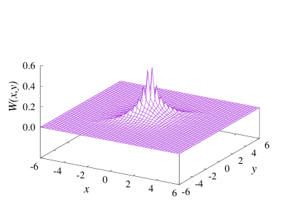
Figure 1: Joint distributions for $c=4$, $h_{0}/J=0.2$ and $\Delta/J=0.0$. Top: $T/J=0.8$, PM phase, RS-stable diagonal distribution. Bottom: $T/J=0.6$, SG phase, RS-unstable non-diagonal distribution.

In the PM phase the system is ergodic, and the RS solution is stable. As mentioned above, the correspondent joint distribution is diagonal, as is shown in the top panel of Figure 1. Conversely, the ergodicity is broken in the SG phase, i.e., this phase is RS unstable, and the joint distribution is no longer diagonal, as can be seen in the bottom panel of Figure 1. We proceed by considering that the SG to PM transition coincides with the AT line.

Representative examples of how the order parameters $q$ and $q^{\prime}$ behaves as the temperature varies is shown in Figure 2, for $c=4$ and two sets of parameters $(h_{0},\Delta,J_{0})$. The set $(0.15,0,0.5)$, representing an example of uniform magnetic field and random couplings with a ferromagnetic constant, is shown in solid lines. The set $(0,0.2,0)$, representing an example fully disordered magnetic local fields and couplings, is shown in dashed lines. This figure reveals that the whole behavior is robust against changes on the parameters, with ergodicity being broken at low temperature.

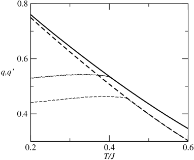
Figure 2: $q$ (thick lines) and $q^{\prime}$ (thin lines) vs. $T/J$ for $c=4$, $h_{0}=0.15$, $\Delta=0$, $J_{0}=0.5$ (solid lines) and $h_{0}=0$, $\Delta=0.2$ and $J_{0}=0$ (dashed lines).

A more complete view of the role played by the random field and average connectivity on finite connectivity spin-glasses is revealed through the phase diagrams. In Figure 3, $T/J$ vs. $J_{0}/J$ phase diagrams for $c=4$, $c=8$ and the fully connected network, with random field and without random field are presented. The SG to PM transition, as well as the transition from the mixed phase FM’ to FM are AT lines, i.e., lines that signal the locus where the ergodicity is broken, with $q$ and $q^{\prime}$ becoming different. The FM’ to SG and F to PM transitions are signaled by the magnetization $m$ going to zero. All the transitions are continuous. The mixed FM’ phase is a non-ergodig ferromagnetic phase, where $m\neq 0$, $q>0$ (it is the correlation of a replica with itself), $q^{\prime}\neq 0$ (it is the correlation between two distinct replicas), and $q\neq q^{\prime}$. As a general remark, when increasing the random field the transition lines are displaced in a way that the surface occupied by more entropic phases increases, and the less entropic phases are reduced. The differences between averages connectivies $c=4$ and $c=8$ are mainly quantitative. When increasing $c$ the transition lines are again displaced, this time in a way the area occupied by the less entropic phases increases, while the more entropic are reduced. So speaking, the SG to PM transition line displaces upwards, the SG to FM’ displaces to the left and FM to PM displaces to the left and FM to FM’ displaces downwards.

It should be remarked that, by comparing finite and fully connectivity, the relevant qualitative difference is that, in the fully connected case, the transition line FM’ to FM goes asymptotically to $T=0$ when $J_{0}/J$ increases, unlike the finite case $c$, where the transition line intersects the $T$ zero axis. This means that a finite connectivity favors the ergodicity at zero temperature.

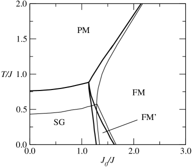
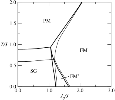
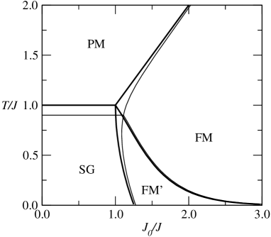
Figure 3: $T/J$ vs. $J_{0}/J$ phase diagrams for $h_{0}/J=0.0$, $\Delta/J=0.0$ (thick lines) and $\Delta/J=0.2$ (thin lines), for $c=4$ (top), $c=8$ (middle) and fully connected (bottom).

Next, we analyze the SG to PM transition through $T/J$ vs. $h_{0}/J$ phase diagrams. Figure 4 shows the SG to PM transitions for connectivity $c=4$ and $c=8$, for four representative values of the field disorder. Although the pictures for different values of $c$ are qualitatively similar, with both the uniform field component $h_{0}$ and the random field component $\Delta$, both given in units of $J$, acting to suppress the SG phase in favor of the PM phase, there are some aspects to consider. First, $\Delta$ is much more effective in suppressing the SG at small than at a large $h_{0}$. Second, it is also more effective the smaller the $c$. This, even considering that both the mean value and the variance of the couplings scale with $c$ (see Eq. 3). This means that a more connected network with weaker couplings produces a more robust SG phase than a less connected network with stronger couplings one. Other aspect that must be very stressed is that the SG phase is suppressed completely above a certain $h_{0}$ for any value of $\Delta$. Moreover, for the same fixed value of $\Delta$, this suppression is much more effective for c=4 than for c=8.

We remark in Figure 4 that the convexity of the curves at small $h_{0}/J$ values changes from $\Delta/J=0$ to $\Delta/J>0$. To investigate this in detail, in Figure 5 we plot, in logarithmic scale, the reduced temperature $\tau=(T_{0}-T)/J$ vs. $h_{0}/J$, for small $h_{0}/J$, where $T_{0}=T(h_{0}/J=0)$, for $\Delta/J=0.00$ and $\Delta=0.01$, with connectivity ranging from $c=4$ to $c=16$. If the reduced temperature is expressed as a power law $\tau\sim(h_{0}/J)^{2/\phi}$ as $h_{0}/J\rightarrow 0$, the slopes in figure indicate that $\phi=2$ for $\Delta/J=0.00$ and $\phi=1$ for $\Delta/J$ as small as 0.01. Here, we compare our results with those obtained for the fully connected network Soares1994 , where $\phi=3$ for $\Delta/J=0.00$, identified as SG regime, and $\phi=1$ for finite $\Delta/J$, identified as the RF regime. We guess that the $\phi=3$ in the SG regime is a particularity of $c\rightarrow\infty$, since the curves for increasing $c$ in Figure 5 superimpose, suggesting that $\phi=2$ in the SG regime is robust for all finite $c$. To resume, the results for both finite and fully connected networks indicates that a crossover from SG to RF regime takes place as $\Delta/J$ becomes non zero.

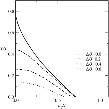
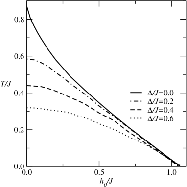
Figure 4: Top: $T/J$ vs. $h_{0}/J$ phase diagrams for $c=4$ and $J_{0}=0$ for different values of $\Delta/J$. Bottom: the same, but for $c=8$.

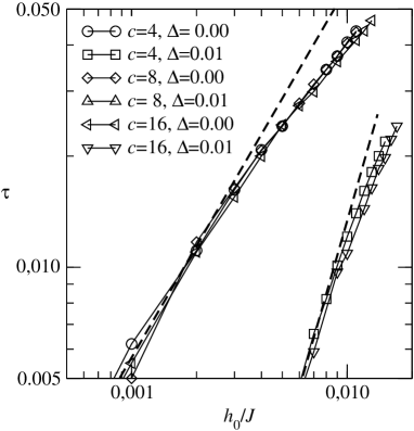
Figure 5: Reduced temperature vs. RF amplitude $h_{0}/J$ for $\Delta/J=0.00$ and $\Delta/J=0.01$, $c=4$, $c=8$ and $c=16$. The solid lines are only guidelines. Shown in dashed, slope 1 and slope 2 straight lines.

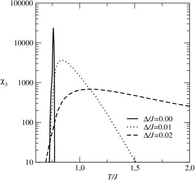
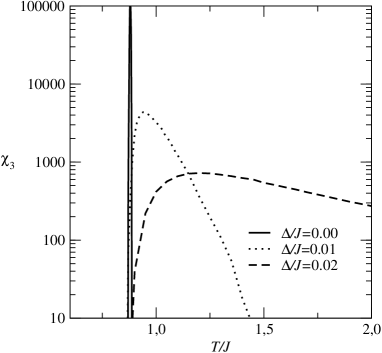
Figure 6: Top: nonlinear susceptibility vs. temperature for $c=4$ and several values of $\Delta/J$. Bottom: the same, but for $c=8$.

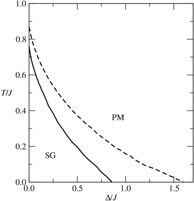
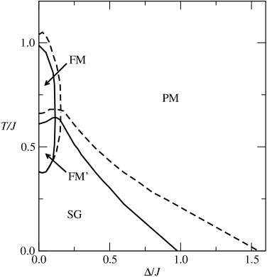
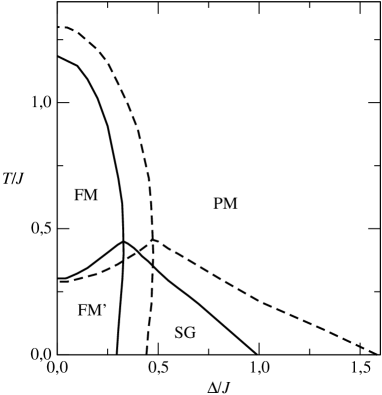
Figure 7: $T/J$ vs. $\Delta/J$ phase diagram for $h_{0}=0$. Top left: $J_{0}/J=0$; $c=4$ (solid lines) and $c=8$ (dashed lines). Top right: $J_{0}/J=1.22$ and $c=4$ (solid lines); $J_{0}/J=1.15$ and $c=8$ (dashed lines). Bottom: $J_{0}/J=1.4$; $c=4$ (solid lines) and $c=8$ (dashed lines). All the transitions are continuous.

Figure 8: Limiting $h_{0}/J$ of the SG phase vs. $c$ at $T=0$, for $\Delta/J=0.0$ and $\Delta/J=0.2$. Below and above the lines are the loci of the SG (non-ergodic) and PM (ergodic), respectively.

The non-linear susceptibility $\chi_{3}=\partial^{3}m/\partial h_{0}^{3}|_{T/J,h_{0}/J=0}$ diverges at the SG to PM transition (AT line) in the SG regime (zero $\Delta/J$) binderyoung . The non-linear susceptibility as a function of $T/J$ is shown in Figure 6, for some small values of $\Delta/J$. For $\Delta/J=0$ indeed there is a divergence at the same $T/J$ where the two-replica method localizes the SG to PM transition, for both $c=4$ and $c=8$. For $\Delta/J>0$ there is a peak instead of a divergence, that no longer signals the SG to PM transition. As $\Delta/J$ increases, the peak becomes quickly less pronounced and moves to higher temperature values, as can be seen in Figure 6.

To complete the description, $T/J$ vs. $\Delta/J$ phase diagrams for $h_{0}/J=0$ and $J_{0}/J$ constant are present in Figure 7. In the top left panel we have $J_{0}/J=0$, that is a prototype for all phase diagrams where the uniform part of the coupling constant is to weak to allow the appearing of ferromagnetic phases. In the top right panel, a constant $J_{0}/J$ in the re-entrant region was chosen. Here, the uniform coupling becomes sufficiently strong to allow the appearing of FM and FM’ phases, although the SG remains as the most ordered phase at zero temperature. For $c=4$ and $c=8$ this takes place, e.g., in the neighborhood of $J_{0}/J=1.22$ and $J_{0}/J=1.15$, respectively. In the bottom panel the $T/J$ vs. $\Delta/J$ phase diagram for a constant $J_{0}/J=1.4$ for both $c=4$ and $c=8$ is shown. Here, the uniform coupling becomes stronger, and the mixed phase FM’ can be found at zero temperature. The phase diagrams are qualitatively similar for both values of the connectivity. All the transitions are continuous. As $\Delta/J$ increases, FM and FM’ phases are the first to be suppressed. Then, the SG to PM transition line decreases monotonically to $T/J=0$ and PM is the only remaining phase at large $\Delta$.

The last comment concerns the comparison with the fully connected network. Here again, the FM’ to FM transition intercepts the zero temperature axis, contrary to the fully connected network. If the two-replica method to localize the AT line is correct, the finite connectivity results should approach the fully connected ones as $c$ increases. This seems to be the case for the general aspects of the phase diagrams shown above, except in the high field and high coupling constant regimes. In the fully connected network there is no paramagnetic phase at zero temperature, in contrast to the finite connectivity case. Note that this does not mean that there is no magnetization at zero $T$: there is, indeed a field-induced magnetization. The main outcome is that we can find the finite connectivity network ergodic at zero $T$, contrary to the fully connectivity network. To illustrate how the zero $T$ ergodicity region evolves as a function of the connectivity is shown in Figure 8. The figure shows the limiting $h_{0}/J$ of the SG phase, at $T=0$. As one should expect, this limit increases slowly but monotonically with $c$.

III Conclusions

In this work we have investigated the problem of the joint presence of SG and RF using random network. In order to accomplish that, we have considered the Random Network Random Field Ising Model Doria where the spin exchange interaction as well as the RF are random variables following a gaussian distribution. Our goal has been, using the connectivity as a control parameter in the theory, to verify whether and which are the differences with the mean field theory i.e., the fully connected theory Soares1994 . Particularly, in the presence of a magnetic field. As a methodological novelty in the problem, we performed the check of the stability of the RS solution using the Two-replica method. This procedure, which gives the AT line, has been used for the SG problem without RF. Thus, in fact, it can be considered that our work also belongs to a more general discussion concerning the description of the SG non-trivial ergodicity breaking using the AT line when the network connectivity can vary.

Following a population dynamics algorithm, the effective distribution of local fields was determined, allowing to the calculation of relevant order parameters. Then, we obtained phase diagrams temperature versus ferromagnetic exchange interaction $J_{0}$ (see Eq. (3)) and temperature versus the magnetic field $h_{0}$ (see Eq. (4)) for several values of the random field variance $\Delta$ and for two values of the average connectivity, namely $c=4$ and $c=8$. All energy scales in the problem are given in units of the variance $J$ of the random exchange spin interaction. The differences in the phase diagrams with the two values of $c$ are mainly quantitative. Nevertheless, the results have shown that the less entropic phases occupy growing areas to the detriment of the more entropic ones as $c$ increases. This means that the connectivity favors the ordered phases, even considering that the coupling constant is correctly normalized with $c$ (see Eq. 3). Moreover, we do remark that the AT line intercepts both the $J_{0}$ and $h_{0}$ axis at zero temperature, contrary to the observed in the fully connected theory. In other words, the SG ground state prevails only within a certain interval of $J_{0}$ and $h_{0}$. This also means that, even with quenched disorder, for finite connectivity there is a region at zero temperature where the ergodicity remains unbroken above a given value of the magnetic field, no matter the strength of the RF gaussian variance $\Delta$. We notice that, in the limit of large values of $c$, there are indications that the fully connected theory is recovered, particularly with regard to the AT line.

To conclude, one of the main outcomes of the present investigation concerns the crossover between the RF and the SG regime. Within the fully connected theory, the crossover between the RF and SG regimes was described by $\tau\equiv T_{0}-T\sim h_{0}^{2/\phi}$ ($T_{0}$ is the freezing temperature without field). In the fully connected theory, the values $\phi=1$ and $3$ corresponds to RF and SG regimes, respectively. We found, in this work, that at small $h_{0}$, $\tau\sim h_{0}$ at $\Delta=0$ and $\tau\sim h_{0}^{2}$ for any finite $\Delta$. In other words, $\phi=1$ and $\phi=2$ in the RF and SG regimes, respectively.

Appendix

The finite connectivity replica method has become standard. We rewrite here only some key points and refer to Mo98 ; ETM for details. After averaging over $c_{ij}$ we obtain, in the $c/N\rightarrow 0$ limit,

$$\left\langle Z^{n}\right\rangle_{\{J_{ij},h_{i},c_{ij}\}}=\sum_{\mbox{\boldmath$\sigma$}^{1}\cdots\mbox{\boldmath$\sigma$}^{n}}\Bigl{\langle}\exp\Bigl{[}\beta\sum_{i,\alpha}h_{i}\sigma_{i}^{\alpha}+\frac{c}{2N}\sum_{i,j\neq i}\Bigl{(}\mathrm{e}^{\beta J_{ij}\mbox{\boldmath$\sigma$}_{i}\cdot\mbox{\boldmath$\sigma$}_{j}}-1\Bigr{)}\Bigr{]}\Bigr{\rangle}_{\{J_{ij},h_{i}\}}\,.$$ (12)

Next, we introduce the fraction $P(\mbox{\boldmath$\sigma$})$ of sites where the replica configuration $\sigma$ is realized and the auxiliary variables $\hat{P}(\mbox{\boldmath$\sigma$})$ and evaluate the trace over the spin variables. This reduces to the problem of one site, and the replicated partition function can be rewritten as

$$\left\langle Z^{n}\right\rangle_{\{J_{ij},h_{i},c_{ij}\}} =\int\prod_{\mbox{\boldmath$\sigma$}}dP\left(\mbox{\boldmath$\sigma$}\right)d\hat{P}\left(\mbox{\boldmath$\sigma$}\right)\exp\Bigl{\{}N\log\sum_{\mbox{\boldmath$\sigma$}}\Big{\langle}\exp\Big{[}\beta h\sum_{\alpha}\sigma^{\alpha}-\hat{P}\left(\mbox{\boldmath$\sigma$}\right)\Big{]}\Big{\rangle}_{h}$$

$$+N\sum_{\mbox{\boldmath$\sigma$}}\hat{P}\left(\mbox{\boldmath$\sigma$}\right)P\left(\mbox{\boldmath$\sigma$}\right)+\frac{Nc}{2}\sum_{\mbox{\boldmath$\sigma$}\mbox{\boldmath$\sigma$}^{\prime}}P\left(\mbox{\boldmath$\sigma$}\right)P\left(\mbox{\boldmath$\sigma$}^{\prime}\right)\Bigl{\langle}\Bigl{(}\mathrm{e}^{\beta J\mbox{\boldmath$\sigma$}\cdot\mbox{\boldmath$\sigma$}^{\prime}}-1\Bigr{)}\Bigr{\rangle}_{J}\Bigr{\}}\,.$$ (13)

In the limit $N\rightarrow\infty$, the saddle-point method applies, and the free-energy becomes

$$f(\beta)=-\lim_{n\rightarrow 0} \frac{1}{\beta n}\mathrm{Extr}_{P(\mbox{\boldmath$\sigma$})}\Bigl{\{}-\frac{c}{2}\sum_{\mbox{\boldmath$\sigma$}\mbox{\boldmath$\sigma$}^{\prime}}P(\mbox{\boldmath$\sigma$})P(\mbox{\boldmath$\sigma$}^{\prime})\Bigl{\langle}\Bigl{(}\mathrm{e}^{\beta J\mbox{\boldmath$\sigma$}\cdot\mbox{\boldmath$\sigma$}^{\prime}}-1\Bigr{)}\Bigr{\rangle}_{J}$$

$$+\log\sum_{\mbox{\boldmath$\sigma$}}\Bigl{\langle}\exp\Bigl{[}\beta h\sum_{\alpha}\sigma^{\alpha}+c\sum_{\mbox{\boldmath$\sigma$}^{\prime}}P(\mbox{\boldmath$\sigma$}^{\prime})\Bigl{\langle}\Bigl{(}\mathrm{e}^{\beta J\mbox{\boldmath$\sigma$}\cdot\mbox{\boldmath$\sigma$}^{\prime}}-1\Bigr{)}\Bigr{\rangle}_{J}\Bigr{]}\Bigr{\rangle}_{h}\Bigr{\}}\,,$$ (14)

where the auxiliary variables $\hat{P}(\mbox{\boldmath$\sigma$})$ were eliminated by the saddle-point equations $\partial f(\beta)/\partial P(\mbox{\boldmath$\sigma$})=0$. The variables $P(\mbox{\boldmath$\sigma$})$ must satisfy the remaining saddle-point equations,

$$P(\mbox{\boldmath$\sigma$})=\dfrac{\Bigl{\langle}\exp\Bigl{[}\beta h\sum_{\alpha}\sigma^{\alpha}+c\sum_{\mbox{\boldmath$\sigma$}^{\prime}}P(\mbox{\boldmath$\sigma$}^{\prime})\Bigl{\langle}\Bigl{(}\mathrm{e}^{\beta J\mbox{\boldmath$\sigma$}\cdot\mbox{\boldmath$\sigma$}^{\prime}}-1\Bigr{)}\Bigr{\rangle}_{J}\Bigr{]}\Bigr{\rangle}_{h}}{\sum_{\mbox{\boldmath$\sigma$}^{\prime}}\Bigl{\langle}\exp\Bigl{[}\beta h\sum_{\alpha}\sigma^{\prime\alpha}+c\sum_{\mbox{\boldmath$\sigma$}^{\prime\prime}}P(\mbox{\boldmath$\sigma$}^{\prime\prime})\Bigl{\langle}\Bigl{(}\mathrm{e}^{\beta J\mbox{\boldmath$\sigma$}^{\prime}\cdot\mbox{\boldmath$\sigma$}^{\prime\prime}}-1\Bigr{)}\Bigr{\rangle}_{J}\Bigr{]}\Bigr{\rangle}_{h}}\,.$$ (15)

We are interested in those solutions satisfying the RS “ansatz”,

$$P(\mbox{\boldmath$\sigma$})=\int dx\,W(x)\frac{\mathrm{e}^{\beta x\sum_{\alpha}\sigma_{\alpha}}}{[2\cosh(\beta x)]^{n}}\,.$$ (16)

This expression is equivalent under permutation of replicas. Introducing the RS ansatz in Eq. (15), we obtain a recursive equation for the distribution of effective local fields $W(x)$, Eq. (7).

References

- (1) A. P. Young (ed), Spin Glasses and Random Fields (Singapore: World Scientific), (1998).
- (2) J. Slak, R. Kind, R. Blinc, E. Courtens, S. Zumer, Phys. Rev. B 30, 85 (1984).
- (3) D. P. Belanger, H. Yoshizawa, Phys. Rev. B 47, 5051 (1993).
- (4) W. Wu, D. Bitko, T. F. Rosenbaum, G. Aeppli, Phys. Rev. Lett. 71, 1919 (1993).
- (5) S. M. A. Tabei, M. P. J. Gingras, Y.-J. Kao, P. Satsiak, J.-Y. Fortin, Phys. Rev. Lett. 95, 237203 (2006).
- (6) R. Pirc, B. Tadic, R. Blinc, Phys. Rev. B 36, 8607 (1987).
- (7) C. A. Morais, F. M. Zimmer, M. J. Lazo, S. G. Magalhaes, F. D. Nobre, Phys. Rev. B 93, 224206 (2016).
- (8) S. G. Magalhaes, C. A. Morais, F. M. Zimmer, M. J. Lazo, F. D. Nobre, Phys. Rev. B 95, 064201 (2017).
- (9) R. F. Soares, F. D. Nobre and J. R. L. de Almeida, Phys. Rev. B 50, 6151 (1994).
- (10) D. Sherrington and S. Kirkpatrick, Phys. Rev. Lett. 35, 1792 (1975).
- (11) J. R. L. de Almeida and D.J. Thouless, J. Phys. A 11, 983 (1978).
- (12) G. Parisi, Phys. Rev Lett. 43, 1754 (1979).
- (13) D. S. Fisher, D. A. Huse, Phys. Rev. Lett. 56, 1601 (1985).
- (14) A. P. Young, H. G. Katzgraber, Phys. Rev. Lett. 93, 207203 (2004).
- (15) A. P. Young, J. Phys. A: Math. Theor. 41, 324016 (2008).
- (16) J. A. Mydosh, Rep. Prog. Phys. 78, 052501 (2015).
- (17) R. Monasson, J. Phys. A: Math. Gen. 31, 513 (1998).
- (18) R. Erichsen Jr., W. K. Theumann and S. G. Magalhaes, Phys. Rev. E 87, 012139 (2013).
- (19) I. Neri, F. L. Metz and D. Bollé, J. Stat. Mech. 2010, P01010 (2010).
- (20) I. Perez Castillo, N. Skantzos, J. Phys. A: Math. Gen. 37, 9087 (2004).
- (21) F.F. Doria, R. Erichsen Jr., D. Dominguez, Mario González, S.G. Magalhaes, Physica A 422, 58 (2015).
- (22) A. Aharony, Phys. Rev. B 18, 3318 (1978).
- (23) S. Magalhaes, C. V. Morais, F. D. Nobre, J. Stat. Mech. 2011, P07014 (2011).
- (24) C. Kwon, D. J. Thouless, Phys. Rev. B 43, 8379, (1991).
- (25) K. Binder and A. P. Young, Rev. Mod. Phys. 58, 801 (1986).
- (26) G. Parisi, F. Ricci-Tersenghi and T. Rizzo, J. Stat. Mech. 2014, P04013 (2014).
- (27) F. Morone, G. Parisi and F. Ricci-Tersenghi, Phys. Rev. B 89, 214202 (2014)