A supra-massive population of stellar-mass black holes in the globular cluster Palomar 5

Abstract

Palomar 5 is one of the sparsest star clusters in the Galactic halo and is best-known for its spectacular tidal tails, spanning over 20 degrees across the sky. With $N$-body simulations we show that both distinguishing features can result from a stellar-mass black hole population, comprising $\sim 20\%$ of the present-day cluster mass. In this scenario, Palomar 5 formed with a ‘normal’ black hole mass fraction of a few per cent, but stars were lost at a higher rate than black holes, such that the black hole fraction gradually increased. This inflated the cluster, enhancing tidal stripping and tail formation. A gigayear from now, the cluster will dissolve as a 100% black hole cluster. Initially denser clusters end up with lower black hole fractions, smaller sizes, and no observable tails. Black hole-dominated, extended star clusters are therefore the likely progenitors of the recently discovered thin stellar streams in the Galactic halo.

ICREA, Pg. Lluís Companys 23, E08010 Barcelona, Spain

Institut de Ciències del Cosmos (ICCUB), Universitat de Barcelona (IEEC-UB), Martí i Franquès 1, E08028 Barcelona, Spain

Department of Physics, University of Surrey, Guildford, GU2 7XH, Surrey, UK

Gravity Exploration Institute, School of Physics and Astronomy, Cardiff University, Cardiff, CF24 3AA, UK

Kapteyn Astronomical Institute, University of Groningen, Postbus 800, NL-9700AV Groningen, The Netherlands

Institute for Astronomy, University of Edinburgh, Royal Observatory, Blackford Hill, Edinburgh EH9 3HJ, UK

Centre for Statistics, University of Edinburgh, School of Mathematics, Edinburgh EH9 3FD, UK

In recent years, a few dozen thin ($\lesssim 100$ pc) stellar tidal streams have been discovered in the Milky Way halo[1, 2, 3, 4]. Their elemental abundances and distribution in the Galaxy provide important constraints on the formation of the Galaxy and its dark matter distribution[5]. Their narrow widths imply that their progenitor stellar systems had a low velocity dispersion and were dark matter-free star clusters rather than dark matter-dominated dwarf galaxies. However, a progenitor has not been found for any of these streams and the star cluster nature is questioned by two recent findings: firstly, the inferred mass-loss rate of the GD-1 stream is several times higher[6] than what is found in frequently cited models of cluster evolution[7] and secondly, only mild tidal distortions and no tidal tidal tails were found[8] for several globular clusters (GCs) with extremely radial orbits[9] passing through the strong tidal field near the Galactic center where tidal stripping is efficient. These results raise the questions of what drove the escape rate of the streams’ progenitors and why this mechanism is not active in all star clusters.

The metal-poor GC Palomar 5 (hereafter Pal 5) is one of the few known star clusters with extended tidal tails associated with it[10], spanning $\gtrsim 20~{}$degrees on the sky, making it a Rosetta stone for understanding tidal tail/stream formation. The cluster has an unusually large half-light radius of $\sim 20$ pc[11] and combined with its relatively low mass of $\sim 10^{4}~{}M_{\odot}$, its average density is among the lowest of all Milky Way GCs: $\sim 0.1~{}M_{\odot}/{\rm pc}^{3}$, comparable to the stellar density in the solar neighbourhood. A low density facilitates tidal stripping and the formation of tidal tails[12], but it is not known whether this low density is the result of nature, or nurture.

It has been proposed that Pal 5 simply formed with a low density[12] and has always been a collisionless system, meaning that two-body interactions were not important in its evolution. However, some properties of Pal 5 are reminiscent of other GCs, such as a spread in sodium abundances[13] and a flat stellar mass function[11]. These features have been attributed to high initial densities[14, 15] and collisional evolution[7] and suggest that Pal 5 in fact is, or was, a collisional stellar system, like the rest of the Milky Way GCs[16]. In this study we aim to reconcile the low density of Pal 5 with collisional evolution.

Since the discovery of gravitational waves[17], updated metallicity-dependent stellar wind and supernova prescriptions have been implemented in GC models[18, 19]. In these models, a large fraction of black holes (BHs) that form from massive stars have masses above $20~{}M_{\odot}$ and do not receive a natal kick, as the result of fallback of material, damping the momentum kick resulting from asymmetries in the supernova explosion [20, 21]. The presence of a BH population in a star cluster accelerates its relaxation driven expansion[22, 23] and escape rate[24, 25]. Observational motivation for considering the effect of BHs on GC evolution stems from the discovery of accreting BH candidates in several GCs with deep radio observations[26, 27] and a BH candidate in a detached binary in NGC 3201[28]. Here we investigate the possibility that Pal 5 was much denser in the past and that the present-day structure and prominent tidal tails are the result of a BH population.

Results

We perform star-by-star, gravitational $N$-body simulations with nbody6++gpu[29]. All clusters are evolved for 11.5 Gyr on the orbit of Pal 5 in a three-component Milky Way (bulge, disc, halo) and the simulations include the effect of stellar and binary evolution. No primordial binaries were included. We consider two prescriptions for BH natal kicks. First we consider the most up-to-date BH recipes[30], in which approximately 73% of the mass of the BH population is retained after natal kicks, almost independently of the initial escape velocity of the cluster (see Methods). Then we test the collisionless hypothesis and draw BH kick velocities from a Maxwellian with the same dispersion as that of neutron stars (NSs). Because we need lower densities for these models, all BHs are ejected by the natal kicks in almost all models (in four models a single BH was retained). The latter approach is similar to that of Dehnen et al.[12], with the added effect of stellar evolution and a direct summation code to correctly include the effect of two-body interactions. We will refer to these two sets of models as wBH and noBH, respectively. The initial parameters and all results are summarised in Tables 1 and 2.

We vary the initial number of stars ($N_{0}$) and the initial mass density within the half-mass radius: $\rho_{\rm h0}\equiv 3M_{0}/(8\pi r_{\rm h0}^{3})$, where $M_{0}\simeq 0.64~{}M_{\odot}\times N_{0}$ is the initial mass and $r_{\rm h0}$ is the initial half-mass radius. We search for a model that best reproduces the observed number of stars of Pal 5, $N_{\rm cluster}=1,550$, and its half-light radius, $R_{\rm eff}=3.21~{}$arcmin/$18.7~{}$pc (see Methods). $R_{\rm eff}$ is defined as the distance to the cluster center containing half the number of observed stars. We first run a coarse grid of models, followed by a finer grid close to the parameters that give the best match in the coarse grid. The best wBH model (wBH-1) has $N_{0}=2.1\times 10^{5}$ and $\rho_{\rm h0}=80~{}M_{\odot}/{\rm pc}^{3}$. This cluster lost 92% of its initial mass of $1.34\times 10^{5}~{}M_{\odot}$ by stellar evolution and escapers and the density decreased nearly three orders of magnitude because of stellar evolution and dynamical heating by BHs. We note that the half-mass radius $r_{\rm h}\simeq 18.8~{}$pc, as determined from the 3-dimensional mass distribution, is similar to $R_{\rm eff}=18.2~{}$pc, which is determined from the projected distribution of observable stars. If mass follows light, $R_{\rm eff}\simeq 0.75r_{\rm h}$ and for mass segregated clusters without BHs it can be as small as $0.5r_{\rm h}$[31]. The fact that $R_{\rm eff}\simeq r_{\rm h}$ for wBH-1 implies that the observable stars are less concentrated than the mass profile. This is the result of the BH population which sinks to the center via dynamical friction against the lower mass stars[22, 23, 32], where they remain in a quasi-equilibrium distribution[33]. The surface density profile and the properties of the stream are in good agreement with the observations (Figure 1). The small-scale density variations in the tails are not reproduced by our model (see Supplementary Figure 1). This is because they are likely the result of interactions with dark matter subhalos[34] or the Galactic bar and giant molecular clouds in the disc[35], which are not included in our model. The observed line-of-sight velocity dispersion of stars in the tails is $2.1\pm 0.4$ km/s[36], which is well reproduced by wBH-1 ($2.4\pm 0.1$ km/s, for giants in the same region as the observations). The most striking property of wBH-1 is its large BH fraction at present: $f_{\rm BH}=22\%$. We define $f_{\rm BH}$ as the total mass in BHs that are bound to the cluster over the total bound cluster mass, that is, $f_{\rm BH}=M_{\rm BH}/M$. The BH population is made up of 124 BHs with an average mass of $17.2~{}M_{\odot}$ (that is, $M_{\rm BH}=2,178~{}M_{\odot}$), currently residing within $R_{\rm eff}$ (see Figure 1). This $f_{\rm BH}$ is more than twice as large as what is expected from a canonical stellar initial mass function (IMF) and stellar evolution alone, and is the result of the efficient loss of stars over the tidal boundary, while the BHs were mostly retained because they are in the center.

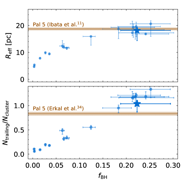
Figure 3: Dependence of cluster and stream properties on the BH content. Effective radius (top) and the relative number of stars in the trailing tail (bottom) for all surviving wBH clusters when their mass is $0.95\times 10^{4}~{}M_{\odot}$ (the mass of wBH-1 at 11.5 Gyr) as a function of $f_{\rm BH}$ (blue dots with error bars). Observed values[11, 34] are shown as horizontal lines with the shaded region indicating the 1$\sigma$ confidence interval. Values of wBH-1 are shown by large stars. Here $N_{\rm trailing}$ is defined as the number of observable stars in the trailing tail, within 4^∘ of right ascension of Pal 5, which in the model corresponds to stars that escaped in the preceding $\sim 1$ Gyr. Because these quantities vary along the orbit at these low masses, we plot the range within the nearest peri and apo as error bars. The strong correlation of both quantities with $f_{\rm BH}$ suggests that for a given orbit and cluster mass, the BH content sets both $R_{\rm eff}$ of the cluster and the prominence of the tidal tails.

In all wBH models, $f_{\rm BH}$ increases in the first $\sim 10$ Myr because of BH formation and stellar evolution mass loss. Then, $f_{\rm BH}$ decreases in the following $\sim 100$ Myr because of BH ejections from the core[33]. This happens because binary BHs form and interact with other BHs when two-body relaxation becomes important. These binaries become more bound in these interactions, eventually ejecting BHs and themselves from the cluster. What happens next depends on $\rho_{\rm h0}$: in dense clusters, most BHs are ejected before the cluster dissolves and these GCs have escape rates and $R_{\rm eff}$ comparable to what is found in models of clusters without BHs (Figure 2). Clusters with lower initial densities have larger relaxation times, resulting in fewer BH ejections, while tidal stripping of stars is more efficient, leading to an increasing $f_{\rm BH}$ until $100\%$[37] (Figure 2). For $f_{\rm BH}\gtrsim 0.1$, $R_{\rm eff}\sim 15$ pc, comparable to what is found for about half of the GCs in the outer halo of the Milky Way[38], suggesting that these ‘fluffy’ GCs are BH rich and candidates to produce prominent stellar streams. This idea is further supported by the strong correlation between $f_{\rm BH}$ and $R_{\rm eff}$ and the fraction of stars in the stream (Figures 3 and 4). Theory suggests[33] that in idealised single-mass star clusters that fill their tidal radius there exists a critical $f_{\rm BH}\simeq 10\%$ at which the mass-loss rate of stars and BHs is the same and $f_{\rm BH}$ remains constant at $10\%$ while the cluster loses mass. For higher(lower) $f_{\rm BH}$, stellar mass is lost at a higher(lower) rate by tidal striping than BH mass is lost by ejections from the core. This implies that clusters can evolve to 100% BH clusters if they form with $f_{\rm BH}\gtrsim 10\%$ and can remain above it during their evolution. Our models suggest that for multimass models this critical fraction is lower: $\sim 2.5\%$. Since for a canonical IMF the initial $f_{\rm BH}\simeq 5-10\%$, depending on metallicity, it is possible for some GCs to remain above the critical $f_{\rm BH}$ and evolve to 100% BH clusters[37], as we find in our wBH-1 model. Because $f_{\rm BH}$ always evolves away from 10%, the distribution of $f_{\rm BH}$ values of a GC population becomes bimodal. Whether cluster evolve towards BH-free clusters, or 100% BH clusters depends on their initial density relative to the tidal density. Because $f_{\rm BH}$ affects the density, a unimodal initial density distribution can evolve towards a bimodal preseny-day density distribution, as is observed in the halo[38].

We now discuss the noBH models. The best-fit model (noBH-1) has $N_{0}=3.5\times 10^{5}$ and $\rho_{\rm h0}=9.625~{}M_{\odot}/{\rm pc}^{3}$, that is, approximately twice as massive and an order of magnitude less dense than wBH-1. The resulting observable parameters $N_{\rm cluster}(R_{\rm eff})$ are within $27\%(5\%)$ of the values of Pal 5. The resulting cluster density profile and stream properties are similar to those of wBH-1 (Supplementary Figure 1), hence based on these observables it is not possible to prefer either of the assumptions for BH kicks. The wBH-1 model predicts a higher central velocity dispersion of 580 m/s vs. 350 m/s for noBH-1 (see Methods). The inferred central dispersion from the literature compilation by Baumgardt & Hilker[39] is $550^{+150}_{-110}~{}$m/s; that is, favouring the BH hypothesis. We quantified the degree of fine-tuning of $N_{0}$ and $\rho_{\rm h0}$ that is required to obtain the best model in both cases. For the wBH models, we find that the uncertainty in the present-day properties can be covered by a relatively large range of initial densities, while for the noBH models we find that variations in the initial density are amplified by more than an order of magnitude in variations in the present-day properties (see Supplementary Information). This means that a relatively large range of initial conditions in wBH models lead to similar present-day properties, while for the noBH models a high degree of fine-tuning in the initial density is required to obtain noBH-1. In addition, noBH-1 completely dissolves at 11.8 Gyr, that is, 300 Myr after we observe the cluster, while wBH-1 survives for another 1.4 Gyr. By assuming simple power-law distributions for the initial cluster masses and densities, we estimate that the probability of finding a cluster with the properties of Pal 5 for wBH-1(noBH-1) is $1/200(1/3.6\times 10^{5})$. Given that the Milky Way has $\sim 150$ GCs, the wBH-1 model provides the more likely explanation for Pal 5. The velocity dispersion and the fine-tuning and timing arguments all favor the BH hypothesis. The final argument in support of the BH hypothesis is that the higher initial density and the resulting collisional nature of Pal 5 make it easier to understand the flat stellar mass function, its multiple populations and its relation to the rest of the Milky Way GC population.

In the observed mass range ($0.6-0.8~{}M_{\odot}$), the mass function of Pal 5 is flatter ($dN/dm\propto m^{\alpha}$, with $\alpha\simeq-0.5$[11]) than what is expected from a canonical IMF ($\alpha=-2.3$), suggesting that Pal 5 has preferentially lost low-mass stars. We note that this result has been questioned and the mass function slope may actually be close to the initial value (Iskren Georgiev, private communication). In Figure 5 we show the mass function of bound stars and remnants of wBH-1. For main sequence stars $>0.5~{}M_{\odot}$ it has a slope of $\alpha=-1.5^{+0.2}_{-0.4}$, which is flatter than the IMF, but steeper than the observed slope. The noBH-1 model has a slope comparable to wBH-1, implying that in the later parts of its evolution the cluster became collisional. The similarity in mass function slope between wBH-1 and noBH-1 means that we can not use the observed mass function to distinguish between the two scenarios. However, in the noBH models the only way to reconcile the models with the observations is to start with a flatter IMF, because the alternative (that is, reducing the initial relaxation timescale by increasing the initial density) leads to a $R_{\rm eff}$ that is too small. The BH scenario, however, leaves the possibility to increase the initial cluster density and still end up with the same present-day BH fraction, $R_{\rm eff}$ and tidal tails. For example, tidal heating by interstellar gas clouds in the early evolution is probably important in the evolution of GCs[40, 41], but this effect is not included in our models. This tidal heating leads to a decrease in the cluster mass[42, 43] and for clusters with a low central concentration the cluster density also decreases[44]. BHs sink to the cluster center by dynamical friction on a fraction of a relaxation time and if this is shorter than the tidal heating timescale, then the BHs are less affected by this mechanism of tidal stripping than the stars, such that $f_{\rm BH}$ increases, counteracting the reduction of $f_{\rm BH}$ from BH ejections from the core due to the higher density. This would be a pathway to start with higher densities. Alternatively, something may have happened to Pal 5 at a later stage of its evolution. It is likely that Pal 5 formed in a dwarf galaxy that was accreted onto the Milky Way, which is supported by its tentative association with the Helmi streams[45]. The cluster could have lost a fraction of its loosely bound stars as a result of the removal of its host galaxy[46], thereby increasing $f_{\rm BH}$. Finally, a flatter IMF at high masses would also lead to a higher $f_{\rm BH}$. This also affects the evolution, because a flatter IMF would lead to faster expansion and a higher mass loss rate[47, 24, 25]. In all these scenarios, denser initial conditions and therefore more equipartition among low-mass stars, whilst ending with the same present-day $f_{\rm BH}$ is a possibility. Understanding the interplay between early mass loss, mass segregation, the (high-mass) IMF and accretion on the Milky Way to find limits on the allowed initial density is an interesting topic for a follow-up study. The initial density is a critical ingredient for our understanding of GC formation[14, 48, 15], evolution[41], BH natal kicks[21] and binary BH mergers[18, 49, 19].

Our results have implications for our understanding of GC evolution. In frequently cited models of cluster evolution without BHs, the relaxation driven escape rate on the orbit of Pal 5 is about $\sim 1~{}M_{\odot}/{\rm Myr}$ (Figure 2). We note that our noBH models have much higher escape rates, but this is because they start with lower initial densities than what is usually done[7]. It is well-established that the mass loss rate in these models is insufficient to ‘turn-over’ a power-law initial cluster mass function with index $-2$, as is observed for young star clusters in the nearby Universe, into the observed peaked (logarithmic) mass distribution with a typical mass of $2\times 10^{5}~{}M_{\odot}$: too many low-mass GCs survive beyond $\gtrsim 5~{}$kpc[50]. The required escape rate is about an order magnitude larger: $20~{}M_{\odot}/{\rm Myr}$[51]. From our models we can conclude that Pal 5 is currently losing mass at that rate (Figure 2), hence if a large fraction of GCs go through a similar evolutionary phase, then relaxation driven evaporation is more important in shaping the GC mass function than usually assumed, reducing the need for additional GC disruption mechanisms[40, 41] or a peaked initial cluster mass function. Because variations in $f_{\rm BH}$ lead to an order of magnitude variation in the escape rate (Figure 2), we conclude that the effect of BHs is of comparable importance in shaping the GC mass function as the details of the Galactic orbit.

Discussion

We now consider our results in the context of the Milky Way GC population. About $10\%$ of the Milky Way GCs have $R_{\rm eff}\gtrsim 10~{}$pc, which led some authors to suggest that two-body relaxation is not important and that their evolution is collisionless[12, 52]. These fluffy GCs are found predominantly at large Galactocentric radii and have low masses ($\lesssim 10^{5}~{}M_{\odot}$). More specifically, beyond $\gtrsim 8~{}$kpc from the Galactic center, half of the GCs have $R_{\rm eff}=10-20$ pc[38]. Our results suggest that these large and low-density GCs are BH rich. Their low densities, relative to the tidal densities on their orbits can be used to constrain their initial densities and masses in a similar way as we did for Pal 5. In wBH-1, about half of the observable stars are lost in the last 3 Gyr and in this period the stream became visible above the background. Combined with the remaining lifetime of $\sim 1$ Gyr, Pal 5 has an observable stream for 30% of its lifetime. There are $26$ low-density GCs beyond 8 kpc from the Galactic center and for about half of them tidal tails or tidal features have been found (Supplementary Table 1). Of these, there are 12 that are at distances comparable to Pal 5, or closer. If we assume that the escape rate is the same for these GCs, combined with the fact the GC mass function is uniform at low masses, then about 30% of these GCs are in the final 30% of their evolution. From this we expect that $\sim 4$ GCs to have prominent tidal tails, providing an explanation for the rarity of Pal 5 and the low-number of known GCs with streams. We can now make an order of magnitude estimate of how many streams the Milky Way fluffy GC population has generated in the past. The $\sim 10$ fluffy, nearby, GCs all have masses below $10^{5}~{}M_{\odot}$, hence the mass function of fluffy clusters is $dN/dM\simeq 10^{-4}~{}M_{\odot}^{-1}$. If these GCs all lose mass at a constant rate of $20~{}M_{\odot}/{\rm Myr}$, then this mass function is constant in time and we expect that these GCs contributed $2\times 10^{-3}$ streams per Myr, or about 20 streams in the last 10 Gyr. This estimate supports the idea that the $\sim 30$[1, 2, 3, 4] known cold streams in the halo resulted from BH-rich, extended GCs that dissolved in the Milky Way halo.

We conclude with a discussion on observational tests of the BH hypothesis. We computed the rate of microlensing events of background quasars in the field of Pal 5 and find that the event rate is too low ($\sim 10^{-8}/$yr). We then looked at the effect of BHs on stellar kinematics and found that it is possible to infer the BHs from the kinematics of the stars. For a BH fraction of 22%, the velocity dispersion of giant stars within $R_{\rm eff}$ is $580~{}$m/s, which is $\sim 200$ m/s higher than for a cluster without BHs (Figure 6). The significance of the available velocity dispersion measurement of $550^{+150}_{-110}~{}$m/s[39] can be improved by increasing the sample of stars, and constraining the properties of binary stars, including their orbital periods. We estimate an upper limit for the periods of binaries with giant stars of $P\simeq 0.5~{}$yr, because longer period binaries were ionised by interactions with BHs. Finding a binary with a larger period would challenge our BH hypothesis, while the absence of such binaries could in combination with additional $N$-body model with primordial binaries be used as support for it. Finally, BHs with stellar binary companions may also exist[28] and could be found from their large velocity variations. A multi-epoch observing campaign to obtain line-of-sight velocities is therefore needed to establish with high precision the central velocity dispersion and the properties of the binaries (see Methods for details). This would provide the critical test of the hypothesis that Pal 5 hosts a $\gtrsim 2\times 10^{3}~{}M_{\odot}$ population of stellar-mass BHs.

Data availability.

A snapshot of the wBH-1 model is published on zenodo (doi:10.5281/zenodo.4739181). All $N$-body data are available upon request.

Code availability.

nbody6++gpu is available from https://github.com/nbodyx/Nbody6ppGPU. limepy is available from https://github.com/mgieles/limepy.

Figure 1: Comparison between the $N$-body model wBH-1 and observations of Pal 5 and its stream. (a) Density profile of observable stars in wBH-1, which provides an excellent match to the observations. There is also good agreement between the stellar stream track (b), the stream density and its gradient (c) and stream width (d) between observations and wBH-1, implying that the rate of escape of stars from Pal 5 and their velocity dispersion in the last few Gyrs are correctly reproduced by wBH-1. The blowout of the cluster shows that almost all of the 124 bound BHs are within $R_{\rm eff}$. All error bars denote the 67% confidence interval.

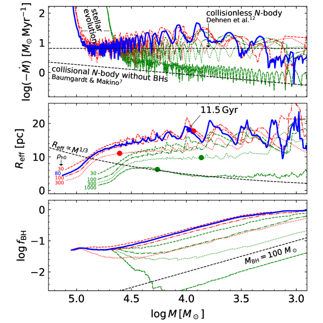
Figure 2: Results for different initial conditions for clusters with BHs. Results of wBH-1 (blue, thick lines), compared to other wBH models with $N_{0}=100k$ (green lines) and $200k$ (red lines) with different initial densities. Different panels show the variation of diagnostic quantities as a function of bound cluster mass ($x$-axis), which decreases in time. Top: Total (positive) mass-loss rate ($-\dot{M}$), which is initially high as the result of stellar evolution. After about 30% of the mass is lost, $\dot{M}$ is dominated by escaping stars and BHs. The results of the collisionless $N$-body model of Pal 5[12] and that of the collisional $N$-body models without BHs[7] are overplotted. Because of the BHs, wBH-1 loses mass at a similar rate as the lower density collisionless models. Middle: Evolution of $R_{\rm eff}$ with the age of 11.5 Gyr indicated with dots. The models do not evolve towards a constant luminosity density (that is, $R_{\rm eff}\propto M^{1/3}$), as predicted for single-mass clusters[53]. Instead, $R_{\rm eff}$ remains approximately constant while the cluster evolves to lower mass and there is a factor of five spread in $R_{\rm eff}$ at a given mass due to variations in $f_{\rm BH}$ (bottom). Dense clusters eject all BHs, while low-density clusters lose stellar mass at a higher rate than BH mass, and evolve along tracks of nearly constant BH mass towards a 100% BH cluster.

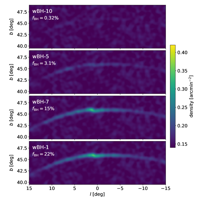
Figure 4: Dependence on stream visibility on BH content. Density map in Galactic latitude ($l$) and longitude ($b$) of unbound stars of four different wBH models (indicated in the top left corners) with different $f_{\rm BH}$ at 11.5 Gyr. A density of background stars of $0.15/{\rm arcmin}^{2}$ was added to each model. Models with $f_{\rm BH}\lesssim 10\%$ do not have prominent tidal tails.

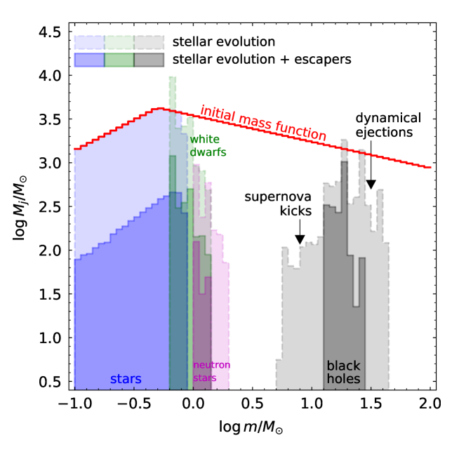
Figure 5: Mass function of stars and remnants. Mass function of bound stars and remnants of wBH-1 at 11.5 Gyr. The mass in each bin ($M_{j}$) is plotted for the IMF, the mass function after only stellar evolution has been applied (light shading) and for the final results of the $N$-body simulation (dark shading). There is a flattening of the stellar mass function due to preferential escape of low-mass stars.

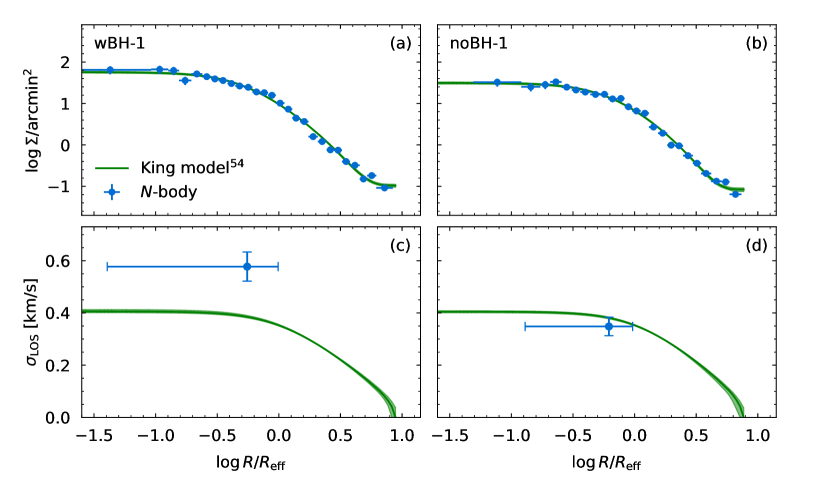
Figure 6: Surface density and velocity dispersion profiles of models with and without BHs. Fits of King models[54] plus a constant background (green lines and shaded region representing the $1\sigma$ uncertainty) to the surface density profile of observable stars (blue circles with error bars indicating the 67% confidence interval) for wBH-1 (a) and noBH-1 (b). (c,d,) The resulting velocity dispersion ($\sigma_{\rm LOS}$) of the model fits scaled to a total mass of $5\times 10^{3}~{}M_{\odot}$ and half-mass radius of $25~{}$pc assuming that the total mass is due to all of the stars, white dwarfs and neutron stars; that is, no BHs. Blue points with error bars in c and d are the dispersions in the $N$-body models of the giants within $R_{\rm eff}$ scaled to the same mass and half-mass radius for wBH-1 and noBH-1, respectively. For noBH-1 the dispersion of the giants is $0.35\pm 0.04$, consistent with the King model prediction. For wBH-1, this dispersion is $0.58\pm 0.06$ km/s, or 3$\sigma$ above the central dispersion prediction from the King model. With precise line-of-sight velocities and a photometric mass estimate, this difference is detectable.

References

MG and EB acknowledge financial support from the European Research Council (ERC StG-335936, CLUSTERS) and MG acknowledges support from the Ministry of Science and Innovation through a Europa Excelencia grant (EUR2020-112157). FA acknowledges support from a Rutherford fellowship (ST/P00492X/2) from the Science and Technology Facilities Council. EB acknowledges financial support from a Vici grant from the Netherlands Organisation for Scientific Research (NWO). MG thanks Mr Gaby Pérez Forcadell for installing the GPU server at the ICCUB on which all the simulations were run. The authors thank Rodrigo Ibata for sharing the data of Pal 5’s surface density profile, Łukasz Wyrzykowski for discussions on microlensing and Sverre Aarseth, Keigo Nitadori and Long Wang for maintaining nbody6 and nbody6++gpu and making the codes publicly available. MG and FA thank Long Wang and Sambaran Banerjee for discussions on the recent sse and bse updates and the implementation in nbody6++gpu. This research made use of astropy, a community-developed core Python package for Astronomy[93, 94], http://www.astropy.org.

M.G. ran all $N$-body simulations, analysed them and was in charge of the writing. D.E. was in charge of stream modelling and deriving the orbit of Pal 5 and the parameters of the MW model. F.A. contributed to the BH physics of the $N$-body models. E.B. converted stream models to observed quantities and J.P. contributed to the binary properties. All authors assisted in the development, analysis and writing of the paper.

The authors have no competing financial interests.

Reprints and permissions information is available at www.nature.com/reprints. Correspondence and requests for materials should be addressed to MG (mgieles@icc.ub.edu).

1.0

Table 1: Overview of the 17 wBH $N$-body simulations of Pal 5. The different columns present: (1) initial number of stars; (2) initial half-mass density; (3) initial mass; (4) initial half-mass radius; (5) age when the cluster had the observed number of stars ($N_{\rm cluster}=1,550$); (6) observable number of stars at 11.5 Gyr; (7) half-light radii at 11.5 Gyr; (8) bound mass at 11.5 Gyr; (9) half-mass radius of the bound stars at 11.5 Gyr; (10) BH mass fraction at an age of 11.5 Gyr; (11) fractional difference with $N_{\rm cluster}$; (12) fractional difference with observed $R_{\rm eff}=18.7\pm 0.4$ pc; (13) overall fractional difference $\delta=\sqrt{\delta_{N}^{2}+\delta_{R}^{2}}$; (14) Model ID, sorted in level of agreement with the data with wBH-1 being the closest match. Dashes are used for models that dissolve before 11.5 Gyr.

(1)	(2)	(3)	(4)	(5)	(6)	(7)	(8)	(9)	(10)	(11)	(12)	(13)	(14)
$N_{0}$	$\rho_{\rm h0}$	$M_{0}$	$r_{\rm h0}$	$T_{\rm 1,550}$	$N_{\rm cluster}$	$R_{\rm eff}$	$M$	$r_{\rm h}$	$f_{\rm BH}$	$\delta_{N}$	$\delta_{R}$	$\delta$	Model
[$10^{3}$]	[$M_{\odot}/{\rm pc}^{3}$]	[$10^{5}M_{\odot}$]	[pc]	[Gyr]		[pc]	[$10^{4}M_{\odot}$]	[pc]	[%]	[%]	[%]	[%]
50	30	0.319	5.04	2.74	–	–	–	–	–	–	–	–	wBH-17
50	100	0.319	3.38	4.06	–	–	–	–	–	–	–	–	wBH-16
50	300	0.319	2.34	5.58	–	–	–	–	–	–	–	–	wBH-14
50	1000	0.319	1.57	8.34	1052	4.05	0.483	5.29	0.701	-32.1	-78.3	84.7	wBH-9
100	30	0.638	6.35	5.40	–	–	–	–	–	–	–	–	wBH-15
100	100	0.638	4.25	7.85	–	–	–	–	–	–	–	–	wBH-13
100	300	0.638	2.95	11.36	1448	9.8	0.732	12.8	3.09	-6.58	-47.6	48	wBH-5
100	1000	0.638	1.97	17.99	3541	6.26	1.84	9.04	0.321	+128	-66.5	145	wBH-10
200	30	1.28	7.98	8.12	–	–	–	–	–	–	–	–	wBH-12
200	100	1.28	5.34	11.43	1399	17.7	0.86	20	20.1	-9.74	-5.3	11.1	wBH-3
200	300	1.28	3.7	17.64	7210	11.1	4.05	14.9	2.75	+365	-40.8	367	wBH-11
210	80	1.34	5.85	11.47	1497	18.1	0.949	18.8	22.3	-3.42	-3.11	4.62	wBH-1
215	80	1.37	5.9	11.13	459	19.9	0.419	15.3	44.6	-70.4	+6.15	70.7	wBH-8
220	70	1.4	6.21	11.45	1411	18.5	0.953	19.8	21.9	-8.92	-0.948	8.97	wBH-2
220	80	1.4	5.94	11.31	791	20.8	0.604	19.4	33	-49	+11.5	50.3	wBH-6
225	70	1.44	6.26	11.29	1091	16.6	0.77	16.5	29.1	-29.6	-11.4	31.7	wBH-4
225	80	1.44	5.98	11.71	2372	16.8	1.45	19.8	15.1	+53.1	-10	54	wBH-7

1.0

Table 2: As in Table 1 but now for the 20 noBH models.

(1)	(2)	(3)	(4)	(5)	(6)	(7)	(8)	(9)	(10)	(11)	(12)	(13)	(14)
$N_{0}$	$\rho_{\rm h0}$	$M_{0}$	$r_{\rm h0}$	$T_{\rm 1,550}$	$N_{\rm cluster}$	$R_{\rm eff}$	$M$	$r_{\rm h}$	$f_{\rm BH}$	$\delta_{N}$	$\delta_{R}$	$\delta$	ID
[$10^{3}$]	[$M_{\odot}/{\rm pc}^{3}$]	[$10^{5}M_{\odot}$]	[pc]	[Gyr]		[pc]	[$10^{4}M_{\odot}$]	[pc]	[%]	[%]	[%]	[%]
100	10	0.638	9.15	7.84	609	4.42	0.289	5.76	0	-60.7	-76.4	97.5	noBH-14
100	30	0.638	6.35	15.09	2682	4.71	1.49	7.24	0	+73.1	-74.8	105	noBH-15
100	100	0.638	4.25	16.71	3607	3.57	2.05	6.33	0	+133	-80.9	155	noBH-18
100	300	0.638	2.95	18.62	4219	4.05	2.16	6.65	0	+172	-78.3	189	noBH-19
200	9.5	1.28	11.7	10.79	1062	8.76	0.501	11.7	0	-31.5	-53.2	61.8	noBH-10
200	10	1.28	11.5	11.65	1675	9.03	0.812	12	0	+8.11	-51.7	52.4	noBH-6
200	30	1.28	7.98	2.35	10320	9.52	6.49	12.7	0	+566	-49.1	568	noBH-20
300	9.5	1.91	13.4	11.11	1065	13.5	0.508	17.5	0.321	-31.3	-27.7	41.8	noBH-5
300	9.625	1.91	13.3	11.38	1349	12.2	0.67	16	0.244	-13	-34.7	37.1	noBH-4
300	9.75	1.91	13.3	11.45	1500	12.2	0.736	16.1	0.222	-3.23	-35	35.1	noBH-3
300	10	1.91	13.2	12.07	2316	12.1	1.2	16.1	0.136	+49.5	-35.5	60.9	noBH-9
350	9.625	2.23	14	11.37	1136	19.6	0.583	25.3	0	-26.7	+4.84	27.1	noBH-1
350	9.75	2.23	14	11.63	1864	13.7	0.966	17.9	0	+20.3	-26.7	33.6	noBH-2
400	9.5	2.55	14.7	11.14	81	22.5	0.0436	33.5	0	-94.8	+20.2	96.9	noBH-12
400	9.625	2.55	14.7	11.40	1105	27.1	0.539	34.7	0	-28.7	+45.1	53.4	noBH-7
400	9.75	2.55	14.6	11.79	2516	14.3	1.28	19.1	0	+62.3	-23.7	66.7	noBH-11
400	10	2.55	14.5	12.16	3237	14.1	1.7	19.1	0	+109	-24.4	112	noBH-16
500	9.5	3.19	15.9	11.14	112	24	0.0573	30.8	0	-92.8	+28.2	97	noBH-13
500	9.75	3.19	15.7	11.66	2429	18.7	1.24	24.6	0	+56.7	+0.0658	56.7	noBH-8
500	10	3.19	15.6	11.92	3650	15.8	1.86	21.1	0	+136	-15.3	136	noBH-17

Methods

Milky Way model and orbit of Pal 5. We adopt a time-independent, axisymmetric Milky Way, consisting of a dark matter (DM) halo, a disc and a bulge. We derive the Milky Way parameters and the orbit of Pal 5 from a fit to the Pal 5 stream. This stream fit is nearly identical to that in Erkal et al.[34] which used the MWPotential2014 potential of Bovy[55], but we use updated priors based on more recent measurements of distance[56] and proper motion[57] of Pal 5 and the distance to the Galactic center[58]. The fit treats Pal 5’s present-day distance, radial velocity, proper motions, the distance to the Galactic center, and the DM-halo mass and scale radius as free parameters.

The DM halo is described by a spherical Navarro-Frenk-White (NFW) profile[59], with potential

$$\Phi_{\rm halo}(R_{\rm G})=-\frac{GM_{\rm NFW}}{R_{\rm G}}\ln\left(1+\frac{R_{\rm G}}{a_{\rm NFW}}\right),$$ (1)

where $R_{\rm G}$ is the Galactocentric radius, $M_{\rm NFW}=4.38713\times 10^{11}~{}M_{\odot}$ is a mass scale and $a_{\rm NFW}=16.043~{}$kpc is the scale radius. For these parameters the virial mass and concentration are $M_{\rm vir}=8.127\times 10^{11}~{}M_{\odot}$ and $c=15.3$, respectively. We note that these parameters are close to those of Bovy[55]. The disc potential is that of an axisymmetric Miyamoto-Nagai disc[60]

$$\Phi_{\rm disc}(R_{\rm G})=-\frac{GM_{\rm MN}}{\left[X^{2}+Y^{2}+\left(a_{\rm MN}+\sqrt{Z^{2}+b^{2}}\right)^{2}\right]^{1/2}},$$ (2)

where $M_{\rm MN}=6.8\times 10^{10}~{}M_{\odot}$ is the mass of the disc, $a_{\rm MN}=3~{}$kpc is the disc scale length and $b=0.28~{}$kpc is the scale height and $X,Y,Z$ are Cartesian Galactocentric coordinates (that is $R_{\rm G}^{2}=X^{2}+Y^{2}+Z^{2}$). The bulge is described by a Hernquist potential[61]

$$\Phi_{\rm bulge}(R_{\rm G})=-\frac{GM_{\rm H}}{R_{\rm G}+a_{\rm H}},$$ (3)

with $M_{\rm H}=5\times 10^{9}~{}M_{\odot}$ the bulge mass and $a_{\rm H}=0.5~{}$kpc its length scale. The bulge model is slightly different from what was used by Erkal et al.[34], but within the orbit of Pal 5 the total enclosed mass of both bulge models is the same.

Cartesian Galactocentric phase-space coordinates of Pal 5 in the potential described above were given by the fit: $[5.733,0.2069,14.34]~{}$kpc and $[-41.33,-111.8,-16.85]~{}$km/s. The Sun is found to be at $[-8.182,0,0]~{}$kpc, with a velocity of $[11.1,245.7,7.3]~{}$km/s, which puts Pal 5 at a distance from the Sun of 19.98 kpc. To find the initial position and velocity of Pal 5’s orbit, we flipped the sign of the velocity vector and integrated the orbit backward in time. We adopt an age of 11.5 Gyr[62, 63, 64] and fix this for all models. The typical uncertainty on the age determinations is $\sim 1$ Gyr and varying the age would somewhat increase the uncertainty on our initial parameters, but not the parameters of our best model. The initial Galactocentric position and velocity of Pal 5 are $[1.212,10.08,2.744]$ kpc and $[43.16,-162.6,147.0]$ km/s, respectively.

Cluster initial conditions and $N$-body code. The initial positions and velocities of the stars were sampled from an isotropic Plummer model[65], truncated at 20 scale radii. Initial stellar masses were sampled from a Kroupa IMF[66] in the range $0.1-100~{}M_{\odot}$ and a metallicity of $Z=6\times 10^{-4}$ was adopted, that is ${\rm[Fe/H]}\simeq-1.4$[13]. All simulations were run with the direct (that is, no softening) $N$-body code nbody6++gpu[67, 68, 29], which deploys a 4^th-order Hermite integrator with an Ahmad-Cohen neighbour scheme[69, 70]. It has recipes for stellar and binary evolution[71, 72], with recent updates for BH masses and kicks[30] and it deals with close encounters with Kustaanheimo-Stiefel (KS) regularisation. We use the Graphics Processing Unit (GPU)-enabled[73] version and the simulations were run on a server with GeForce RTX 2080 Ti GPUs at ICCUB. A few modifications to the code were made for this project. The singular isothermal halo was replaced by the NFW halo, with the force and force derivatives derived from equation (1). Stars were stripped from the simulation when they reached a distance of 40 times the instantaneous half-mass radius of the bound particles and for each escaper the time, position and velocity in the Galactic frame was stored. The escapers were then integrated as tracer particles in the Galactic potential until 11.5 Gyr with a separate integrator to construct the tidal tails. We did not include the contribution of the cluster to the equation of motion of the tail stars. Near the end of the simulation the fractional contribution of the cluster to the total force is approximately $2\times 10^{-5}$ for stars that just left the cluster, and smaller for stars at larger distances, justifying this assumption. All models were evolved until complete dissolution, and for the models that dissolved after 11.5 Gyr, a snapshot was saved at exactly 11.5 Gyr (that is, when the cluster is at the position of Pal 5 today).

Black hole recipes. The fast evolution codes sse[71] for stars and bse[72] for binaries in nbody6++gpu were recently modified[30] with updated prescriptions for wind mass loss, compact object (that is neutron stars and BHs) formation and supernova kicks[21]. We adopt here the rapid supernova mechanism in which the explosion is assumed to occur within the first 250ms after bounce[21], which corresponds to nsflag=3 in sse/bse. The BH natal kick velocities are drawn from a Maxwellian with dispersion $\sigma=265$ km/s[74], and in the wBH models they are subsequently lowered by the amount of fallback such that momentum is conserved (that is, kmech = 1). As a result, 63%(73%) of the number(mass) of BHs does not receive a kick for the IMF and metallicity we used. The BHs that receive a kick form from stars with zero age mean sequence (ZAMS) masses in the range $23-34~{}M_{\odot}$, resulting in BH masses in the range $6-26~{}M_{\odot}$, and because of the low escape velocities of our model clusters (10-20 km/s) they are almost all lost. As a result, the lowest mass BH in the cluster just after supernovae and kicks has a mass of $13~{}M_{\odot}$ and the average BH mass is $21~{}M_{\odot}$.

In natal kick models that consider the effect of fallback of mass on the BH[75], the exact fraction of BHs that do not receive a kick depends on the prescription for compact-object formation. For our IMF and metallicity we find for the StarTrack, rapid, and delayed explosion mechanisms described in section 4 of Fryer et al.[21], that about $83\%$, $73\%$ and $56\%$ of the total BH mass is in BHs that form without a natal kick, respectively. Our result of $73\%$ is therefore an intermediate value. A lower(higher) initial $f_{\rm BH}$ requires a lower(higher) initial cluster density to end up with the same cluster properties at the present day.

Pal 5 parameters. To find the number of observed stars ($N_{\rm cluster}$) and half-light radius ($R_{\rm eff}$) of Pal 5, we fit King models[54] to the density profile of figure 10 of Ibata et al.[76] using limepy[77] and the Markov Chain Monte Carlo (MCMC) code emcee[78]. We fit for the dimensionless central potential: $W_{0}=4.6\pm 0.3$, the number of observed stars: $N_{\rm cluster}=1,550\pm 40$, the half-mass radius: $r_{\rm h}=4.3\pm 0.1~{}$arcmin and the background: $0.07\pm 0.01$ arcmin^-2. For these parameters $R_{\rm eff}=3.21\pm 0.06$ arcmin, which for the adopted distance to Pal 5 of 19.98 kpc corresponds to $R_{\rm eff}=18.7\pm 0.4$ pc.

Data analysis. For each simulation, snapshots were saved approximately every 50 Myr. For each snapshot, we find the stars and remnants that are energetically bound to the cluster, those that have a specific energy $E_{i}=0.5v_{i}^{2}+\phi_{i}<0$, where $v_{i}$ is the velocity in the cluster’s center of mass frame and $\phi_{i}$ is the potential due to the mass of the other bound stars, which we determine iteratively. From the bound particles we determine the total cluster mass $M$, the mass of the BH population $M_{\rm BH}$, the half-mass radius $r_{\rm h}$, $N_{\rm cluster}$ and $R_{\rm eff}$.

To compare the $N$-body models to observations, we use isochrones to convert masses of stars in different evolutionary phases to magnitudes. We use Sloan Digital Sky Survey (SDSS) $g$-band magnitudes from MESA Isochrones and Stellar Tracks (MIST) isochrones[79, 80] for 11.5 Gyr, $Z=6\times 10^{-4}$ (${\rm[Fe/H]}=-1.4$), ${\rm[}\alpha/{\rm Fe]}=0$ and rotational velocities of 0.4 times critical. For the observations shown in Figure 1, Canada-France-Hawaii Telescope (CFHT) photometry was used[81] which is a slightly different photometric system than SDSS. A color transformation is provided by Ibata et al.[81]. For the magnitude limits we adopt here, the colors of Pal 5 stars vary between $0.3\lesssim(g-r)_{\rm CHFT}\lesssim 0.5$ in the relevant magnitude range, resulting in corrections in the $g$-band between $0.07-0.11$. We therefore adopt $g_{\rm SDSS}=g_{\rm CFHT}+0.1$ to convert between the two systems. For the observed number density profile, a magnitude range of $19<g_{\rm CFHT}<23$ was used by Ibata et al.[11]. We apply the corresponding magnitude range $19.1<g_{\rm SDSS}<23.1$ and combined with the adopted distance (DM=16.5 mag) this implies a mass range of main sequence stars of $0.625-0.815~{}M_{\odot}$, which is what we use to select stars in the $N$-body model to construct the surface density profile. For the stream we selected stars with $20.3<g_{\rm CFHT}<23.5~{}$mag (that is $20.4<g_{\rm SDSS}<23.6$) as in Ibata et al.[81]. This magnitude cut implies mass limits that depend on the distance of stars in the tidal tails.

Finding the best model. We varied the initial number of stars $N_{0}$ and the initial half-mass density $\rho_{\rm h0}$ and try to reproduce $N_{\rm cluster}$ and $R_{\rm eff}$. For the wBH models, we first ran a coarse grid of models with $N_{0}=[50k,100k,200k]$ and $\rho_{\rm h0}=[30,100,300,10^{3}]~{}M_{\odot}/{\rm pc}^{3}$. We ran each combination of $N_{0}$ and $\rho_{\rm h0}$, apart from $N_{0}=200k$ and $\rho_{\rm h0}=10^{3}~{}M_{\odot}/{\rm pc}^{3}$. For each model we computed the fractional differences between the $N$-body results and the observations for $N_{\rm cluster}$ and $R_{\rm eff}$ at 11.5 Gyr: $\delta_{N}$ and $\delta_{R}$, respectively, and then define the best model as the one for which $\delta=\sqrt{\delta^{2}_{N}+\delta_{R}^{2}}$ is lowest. For each model we also find the time to reach $N_{\rm cluster}=1,550$ (that is, $T_{\rm 1,550}$). We introduce $T_{1,550}$ to establish a goodness of fit for models that dissolve before 11.5 Gyr. Model IDs are increasing with the value of $\delta$ and for clusters that dissolved the ID is in order of increasing difference between $T_{1,550}$ and 11.5 Gyr. The model with the smallest $\delta$ in the coarse grid has $N_{0}=200k,\rho_{\rm h0}=100~{}M_{\odot}/{\rm pc}^{3}$ and reproduces the two observables within 10%. From the coarse grid we estimate that a slightly larger $N_{0}$ and lower $\rho_{\rm h0}$ would reduce the difference. We then ran a finer grid with 6 more models with $N_{0}$ in the range $210k-225k$ and $\rho_{\rm h0}$ in the range $70-80~{}M_{\odot}/{\rm pc}^{3}$. The model with the smallest $\delta$, wBH-1, has $N_{0}=210k$ and $\rho_{\rm h0}=80~{}M_{\odot}/{\rm pc}^{3}$. It reproduces both observables within 3% and it has a present-day mass of $9.5\times 10^{3}~{}M_{\odot}$, $r_{\rm h}=18.8~{}$pc and $f_{\rm BH}=0.22$. For the noBH models, we first ran five models with $N_{0}=[100k,200k,300k,400k,500k]$ and $\rho_{\rm h0}=10~{}M_{\odot}/{\rm pc}^{3}$, two models with $N_{0}=[100k,200k]$ and $\rho_{\rm h0}=30~{}M_{\odot}/{\rm pc}^{3}$ and two models with $N_{0}=100k$ and $\rho_{\rm h0}=[100,300]~{}M_{\odot}/{\rm pc}^{3}$. Models with $\rho_{\rm h0}=10~{}M_{\odot}/{\rm pc}^{3}$ gave results similar to the observations. We then ran an additional 11 models with densities $\rho_{\rm h0}\lesssim 10~{}M_{\odot}/{\rm pc}^{3}$ and $200k\leq N_{0}\leq 500k$ and found that the model with the lowest $\delta$ has $N_{0}=350k$ and $\rho_{\rm h0}=9.625~{}M_{\odot}/{\rm pc}^{3}$. All model results are summarised in Tables 1 and 2.

Rate of growth of the tidal tails and their visibility. From the escaping stars we find that half of the observable stars in the tails of wBH-1 were ejected in the final 3 Gyr. To estimate the number of MW field stars in Figure 4 that share the same locus in color-magnitude as Pal 5, we use the CFHT data and color-magnitude selection criteria from Ibata et al.[81]. Additionally, we select only stars more than 0.4 deg away from the best-fit stream track from Erkal et al.[34] and adopt their magnitude limits of $20.0<g_{\rm CFHT}<23.5~{}$mag. This sample is dominated by MW field stars and has an average density of 0.142 stars/arcmin². Note that Pal 5 stream runs roughly at a constant $b$ in the region explored in Figure 5, thus variations in the MW field density with position are negligible.

Predictions for observations. To estimate whether the BH population can be detected from the kinematics, we look at the velocity dispersion of the wBH-1 model. Within $R_{\rm eff}$ ($\sim 3.2$ arcmin), there are 40 giant stars, with a line-of-sight velocity dispersion of $0.69\pm 0.09~{}$km/s. Because our wBH-1 model has a steeper mass function than Pal 5, the mass of wBH-1 is likely too high. We therefore scale our model results to a conservative mass of $5\times 10^{3}~{}M_{\odot}$[11] (excluding BHs) and $r_{\rm h}=25~{}$pc. This reduces the predicted dispersion of the giants to $0.58\pm 0.06~{}$km/s. In the noBH-1 model we find 51 giants within $R_{\rm eff}$, which have a (scaled) line-of-sight dispersion of $0.42\pm 0.04~{}$km/s. We then fit King models[54] and a constant background using limepy[77] to the number density profile of bright main sequence stars shown in Figure 1(a). In Figure 6(a,b) we show the results. For wBH-1 we find a dimensionless central concentration of $W_{0}=5.9\pm 0.2$, $r_{\rm h}=27.7\pm{0.8}$ pc, which results in $R_{\rm eff}=20.8\pm 0.6$ pc. For noBH-1 we find $W_{0}=5.2\pm 0.3$, $r_{\rm h}=31.5\pm{1.1}$ pc, which results in $R_{\rm eff}=23.9\pm 0.4$ pc. We then derive the line-of-sight velocity dispersion of the King models by adopting a total mass (excluding the BHs) of: $5\times 10^{3}~{}M_{\odot}$ and $r_{\rm h}=25~{}$pc. The resulting velocity dispersion profiles are shown in Figure 6(c,d). The central dispersion of the King models is $\sim 0.4$ km/s. The dispersion of the giants in the noBH-1 model agrees with this, which means that the derived dispersion provides an accurate measure of the total mass when assuming that the surface density traces the total mass. For the wBH-1 model, however, the dispersion of the giants is about 50% (or 200 m/s) higher. A small part of this difference can be explained by the fact that wBH-1 is a factor of $1/(1-0.22)\simeq 1.3$ more massive, because of the BHs. This higher mass increases the dispersion by a factor of $\sqrt{1.3}\simeq 1.14$. The additional factor of 1.3 needed to explain the dispersion of the giants is because the BHs are centrally concentrated, inflating the central dispersion more than in the mass follows light assumption. Although it is challenging to find a 200 m/s velocity difference, it is feasible with existing high-resolution spectographs ($R\sim 20\,000$) on $8$m-class telescopes with a multi-epoch observing strategy. Baumgardt & Hilker[39] present a compilation of line-of-sight velocities of Milky Way GCs. There are 32 stars in their Pal 5 sample, and the dispersion of the inner 15 stars is $0.55^{+0.15}_{-0.11}~{}$km/s. From a comparison of $N$-body models to the kinematics and surface brightness profiles the authors derive a central dispersion of 0.6 km/s. For such a low dispersion the orbital motions of binary stars are important. The authors have repeat observations for about half of their stars, and they reject stars with large velocity variations. Their result supports the BH hypothesis, but a more thorough analysis of the binary content is desirable. Pal 5 has approximately $50(100)$ stars brighter than $g<19(20)~{}$mag within 3 arcmin from the center for which (additional) line-of-sight velocities can be obtained. For individual measurement errors of 300 m/s and a velocity dispersion of 400 m/s, the estimated uncertainty in the velocity dispersion for 50(100) stars is 63(43) m/s, that is smaller than the difference between wBH-1 and noBH-1. Similar uncertainties can be obtained even when simultaneously fitting on the velocity dispersion and the properties of binary stars[82].

The BH scenario also make a critical prediction for the properties of the binary stars. Soft binaries are ionised when they interact with stars[83] and the binaries with the lowest binding energy are therefore indicators of the most energetic cluster members, including invisible remnants. From wBH-1 we find that the average kinetic energy of the BHs is $\langle K_{\rm BH}\rangle=\langle 0.5mv^{2}\rangle\simeq 10~{}M_{\odot}({\rm km/s})^{2}$, while for all the other stars, white dwarfs and neutron stars we find $\langle K_{*}\rangle\simeq 0.3~{}M_{\odot}({\rm km/s})^{2}$. Adopting circular orbits and equal-mass binary components of $0.8~{}M_{\odot}$ (that is, the mass of giants for which we can obtain velocities) we find that the orbital period is capped at $P_{\rm max}\simeq 2.3\times 10^{4}(120)~{}$yr because of interactions with stars(BHs). However, finding no binaries with $P>120~{}$yr does not confirm the presence of BHs, because the cluster was initially more massive and compact, such that soft binaries had shorter periods. From the initial mass and half-mass radius of wBH-1(noBH-1) we find that the initial $\langle K\rangle$ was a factor of $45(30)$ higher, implying that in the BH case, the maximum binary period is $P_{\rm max}\simeq 0.5~{}$year, while in the noBH hypothesis the maximum period is $P_{\rm max}\simeq 140~{}$yr. This suggests that the presence of binaries with $0.5~{}\lesssim P/{\rm yr}\lesssim 140~{}$ would be an argument against the presence of a BH population, while the absence of such binaries combined with more detailed predictions from $N$-body simulations with primordial binaries could be used as support for the BH case. For $P=[1,10,100]$ yr, the orbital velocities are $[12,5.8,2.7]~{}$km/s, hence these binaries would be easily detectable with a baseline of weeks/months and moderate spectral resolution. In addition, multi-epoch kinematics serves to look for stars with a (detached) BH binary companion such as found in NGC3201[28, 84]. Although dynamical formation of BH binaries is more common, a BH with stellar companion can form in an exchange interaction[85].

We note that several studies have put forward observational signatures of BH populations in clusters by using dynamical models. These studies used either the degree of mass segregation[32, 86, 87, 88] or other observational properties of GCs[89] to make predictions for the size of the BH populations in a subset of Milky Way GCs. None of these studies included Pal 5, so we can not make a comparison. We can check whether these methods would be able to infer the correct BH population given our model properties. From the scaling between $f_{\rm BH}$ and the ratio of core over half-light radius ($R_{\rm core}/R_{\rm eff}$) shown in figure 7 of Weatherford et al.[88] and the ratio $R_{\rm core}/R_{\rm eff}\simeq 0.5$ in wBH-1, we would infer that Pal 5 has a BH population of (only) $f_{\rm BH}\simeq 0.3-1\%$. The reason the inferred $f_{\rm BH}$ from their relation is so different could be because $R_{\rm core}/R_{\rm eff}$ saturates or goes down again for vary large $f_{\rm BH}$ where they have no models, or because of a systematic difference in $R_{\rm core}$ between the Monte Carlo and $N$-body methods[90, 91]. Using the fitted relations provided by Askar et al.[89] (see their Table A1) between the global properties of stellar-mass BHs and the observational properties of their host globular cluster, they find that about 50% of the mass in Pal 5 could be in stellar-mass BHs.

Microlensing event rate. For a BH mass of $17~{}M_{\odot}$ at a distance of 20 kpc, the Einstein angle is $\theta_{\rm E}\simeq 2.6~{}$mas. In wBH-1 there are 124 BHs, mostly within $R_{\rm eff}\simeq 3~{}$arcmin, resulting in a surface density of $\Sigma_{\rm BH}\simeq 1.2\times 10^{-9}~{}$mas^-2. The proper motion of Pal 5 is $\mu\simeq 3.2~{}$mas/yr, such that the event rate for a single background source (that is, an active galactic nucleus) is $\theta_{\rm E}\Sigma_{\rm BH}\mu\simeq 10^{-8}$/yr. In the recent active galactic nuclei catalogue from the Gaia and WISE surveys[92] we find 2 active galactic nuclei within $R_{\rm eff}$ of Pal 5, too low to get to a reasonable event rate. The event rate would be larger if we also consider background halo stars, but even with the estimated density of background galaxies in LSST ($\sim 50/{\rm arcmin}^{2}$), the lensing event rate would be too low ($\sim 10^{-5}/$yr).

Supplementary Information

Sensitivity to initial conditions

We determine how sensitive the final parameters are to variations in the initial parameters. For a quantity $A$, we express the difference between its value for model $i$ ($A^{i}$) and the best model ($A^{1}$) as $\Delta\log A=\log(A^{i}/A^{1})$, where $A$ can be an initial property ($N_{0}$ or $\rho_{\rm h0}$) or an observable property. For the latter we use $N_{\rm cluster}$ and the number density within the half-light radius: $\rho_{\rm eff}=3N_{\rm cluster}/(8\pi R_{\rm eff}^{3})$. We can write the variation in the final properties in terms of the initial properties as

$$\begin{pmatrix}\Delta\log N_{\rm cluster}\\ \Delta\log\rho_{\rm eff}\end{pmatrix}=\Sigma\begin{pmatrix}\Delta\log N_{0}\\ \Delta\log\rho_{\rm h0}\end{pmatrix}.$$ (4)

Here $\Sigma$ is a matrix that contains the constants that relate variations in initial parameter to variations in the final parameters. We find the four elements of $\Sigma$ from the two models that are nearest to the observations (that is, wBH-2, wBH-3 and noBH-2, noBH-3)

$$\Sigma_{\rm wBH}=\begin{pmatrix}-5.74&-1.56\\ -7.19&-1.57\end{pmatrix},\Sigma_{\rm noBH}=\begin{pmatrix}1.47&38.4\\ -0.71&122\end{pmatrix}.$$ (5)

Absolute values of 1 mean that a fractional change in an initial parameter leads to the same fractional change in the final parameter. The absolute values $>1$ in the left column of $\Sigma_{\rm wBH}$ mean that the final properties are most sensitive to $N_{0}$, which is because of the collisional nature of the wBH models. The $>1$ value in the right column of $\Sigma_{\rm noBH}$ show that the final parameters are most sensitive to the initial density, which is because of the collisionless nature of these models. Taking the inverse of the $\Sigma$ matrices, and assuming small variations, that is, $\Delta\log A\simeq\log(1+\epsilon_{A})\propto\epsilon_{A}$, with $\epsilon_{A}<<1$, we can write

$$\begin{pmatrix}\epsilon_{N_{0}}\\ \epsilon_{\rho_{\rm h0}}\end{pmatrix}_{\rm wBH}\simeq\begin{pmatrix}0.711&-0.707\\ -3.26&2.60\end{pmatrix}\begin{pmatrix}\epsilon_{N_{\rm cluster}}\\ \epsilon_{\rho_{\rm eff}}\end{pmatrix}$$ (6)

and

$$\begin{pmatrix}\epsilon_{N_{0}}\\ \epsilon_{\rho_{\rm h0}}\end{pmatrix}_{\rm noBH}\simeq\begin{pmatrix}0.590&-0.186\\ 0.00345&0.00713\end{pmatrix}\begin{pmatrix}\epsilon_{N_{\rm cluster}}\\ \epsilon_{\rho_{\rm eff}}\end{pmatrix}\ .$$ (7)

This shows that the level of fine-tuning to obtain the correct $N_{0}$ is similar in both models, albeit more sensitive to variations in $\rho_{\rm eff}$ for the noBH models. However, we find different behaviour for the initial density, $\rho_{\rm h0}$: for the wBH models, variations in $N_{\rm cluster}$ and $\rho_{\rm eff}$ allow for larger variations in $\rho_{\rm h0}$, meaning that a relatively large range of initial densities can contribute to the error bars on the present-day properties. The results of the noBH models are extremely sensitive to the initial density, because variations in the observed properties correspond to variations of less than a per cent in the initial density. We can also estimate what fraction of the parameter space of the initial conditions is covered by the uncertainties in $N_{0}$ and $\rho_{\rm h0}$. We assume that the initial cluster properties are sampled from power-law distributions with indices $-2$ for $N_{0}$[1] and $-1$ for $\rho_{\rm h0}$[2] in the ranges $10^{5}\leq N_{0}\leq 5\times 10^{6}$ and $1\leq\rho_{\rm h0}/(M_{\odot}\,{\rm pc}^{-3})\leq 10^{4}$. Then we find that the initial conditions of wBH-1(noBH-1) that contribute to the error circle cover a fraction 1/200(1/$3.6\times 10^{5}$) of the initial conditions. Given that the Milky Way has $\sim 150$ GCs, this exercise shows that finding Pal 5 is probable in the wBH scenario, while the probability in the noBH scenario is $10^{-3}$.

Supplementary Figure 1: Comparison of stream properties. Comparison between stream properties of wBH-1 and noBH-1 and the observed stream from Erkal et al.[3]. The stream width (top) of both $N$-body models is similar over the range included in the observations and shows some systematic deviations from the observed width. The density profile (bottom) of the $N$-body models is smoother than the observed profile, which shows signatures of over/under-densities. The decline in the density of the trailing arm (large RA) is faster in wBH-1 than in noBH-1, which agrees more with the observed decline. Shaded regions indicate the 67% confidence intervals.

1.0

Table 3: *

compact GCs			‘fluffy’ GCs
name	distance [kpc]	tail data	name	distance [kpc]	tail data
NGC 3201	4.9	long tidal tails[4, 5]	NGC 288	8.9	long tidal tails[6, 7, 4]
NGC 6205	7.1	tidal tails[8]	Pal 1	11.1	tidal tails[9]
NGC 6341	8.3	long tidal tails[4]	NGC 6101	15.4	-
NGC 362	8.6	tidal feature[10]	NGC 5466	16.0	tidal tails[11, 12]
NGC 6779	9.4	-	NGC 5053	17.4	tidal feature[13]
NGC 2808	9.6	-	IC 4499	18.8	-
NGC 5272	10.2	-	BH 176	18.9	-
NGC 4590	10.3	long tidal tails[4]	Pal 12	19.0	tidal tails[8]
NGC 7078	10.4	-	NGC 6426	20.6	-
NGC 2298	10.8	tidal features[14]	Rup 106	21.2	-
NGC 7089	11.5	-	ESO 280	21.4	-
NGC 5286	11.7	-	Ter 7	22.8	-
NGC 1851	12.1	long tidal tails[7, 4]	Pal 5	23.2	long tidal tails[15, 16, 4]
NGC 1904	12.9	tidal tails[7]	IC 1257	25.0	-
NGC 6934	15.6	-	Pal 13	26.0	long tidal tails[17]
NGC 1261	16.3	long tidal tails[7, 4]	Ter 8	26.3	-
NGC 5024	17.9	-	NGC 7492	26.3	tidal tails[18]
NGC 6981	17.0	-	Arp 2	28.6	-
NGC 4147	19.4	tidal feature[13]	AM 4	32.2	-
NGC 6864	20.9	-	Pyxis	39.4	-
NGC 5634	25.2	-	Pal 15	45.1	tidal tails[19]
Pal 2	27.2	-	Pal 14	76.5	tidal tails[20]
NGC 6229	30.5	-	Eridanus	90.1	tidal tails[19]
NGC 5824	32.1	-	Pal 3	92.5	tidal feature[21]
NGC 5694	35.0	-	Pal 4	108.7	tidal feature[21]
NGC 7006	41.2	-	AM 1	123.3	-
Supplementary Table 1: Summary of results of stream searches for GCs at distances $>8$ kpc from the Galactic center. The classification ‘compact’ (left) and ‘fluffy’ (right) is from Baumgardt et al.[22]. All clusters are sorted in distance from the Sun. Among the compact clusters, no tidal tails nor tidal features were found for clusters that are more than 20 kpc away, while they were found for about half of the fluffy clusters beyond 20 kpc.

References

References

- [1] Bernard, E. J. et al. A Synoptic Map of Halo Substructures from the Pan-STARRS1 3 Survey. MNRAS 463, 1759–1768 (2016).
- [2] Shipp, N. et al. Stellar Streams Discovered in the Dark Energy Survey. ApJ 862, 114 (2018).
- [3] Malhan, K., Ibata, R. A. & Martin, N. F. Ghostly tributaries to the Milky Way: charting the halo’s stellar streams with the Gaia DR2 catalogue. MNRAS 481, 3442–3455 (2018).
- [4] Ibata, R. A., Malhan, K. & Martin, N. F. The Streams of the Gaping Abyss: A Population of Entangled Stellar Streams Surrounding the Inner Galaxy. ApJ 872, 152 (2019).
- [5] Koposov, S. E., Rix, H.-W. & Hogg, D. W. Constraining the Milky Way Potential with a Six-Dimensional Phase-Space Map of the GD-1 Stellar Stream. ApJ 712, 260–273 (2010).
- [6] de Boer, T. J. L., Erkal, D. & Gieles, M. A closer look at the spur, blob, wiggle, and gaps in GD-1. MNRAS 494, 5315–5332 (2020).
- [7] Baumgardt, H. & Makino, J. Dynamical evolution of star clusters in tidal fields. MNRAS 340, 227–246 (2003).
- [8] Kuzma, P. B., Da Costa, G. S. & Mackey, A. D. The outer envelopes of globular clusters. II. NGC 1851, NGC 5824 and NGC 1261∗. MNRAS 473, 2881–2898 (2018).
- [9] Myeong, G. C., Evans, N. W., Belokurov, V., Sand ers, J. L. & Koposov, S. E. The Sausage Globular Clusters. ApJ 863, L28 (2018).
- [10] Odenkirchen, M. et al. Detection of Massive Tidal Tails around the Globular Cluster Palomar 5 with Sloan Digital Sky Survey Commissioning Data. ApJ 548, L165–L169 (2001).
- [11] Ibata, R. A., Lewis, G. F., Thomas, G., Martin, N. F. & Chapman, S. Feeling the Pull: A Study of Natural Galactic Accelerometers. II. Kinematics and Mass of the Delicate Stellar Stream of the Palomar 5 Globular Cluster. ApJ 842, 120 (2017).
- [12] Dehnen, W., Odenkirchen, M., Grebel, E. K. & Rix, H.-W. Modeling the Disruption of the Globular Cluster Palomar 5 by Galactic Tides. AJ 127, 2753–2770 (2004).
- [13] Smith, G. H., Sneden, C. & Kraft, R. P. A Study of Abundances of Four Giants in the Low-Mass Globular Cluster Palomar 5. AJ 123, 1502–1508 (2002).
- [14] Elmegreen, B. G. Globular Cluster Formation at High Density: A Model for Elemental Enrichment with Fast Recycling of Massive-star Debris. ApJ 836, 80 (2017).
- [15] Gieles, M. et al. Concurrent formation of supermassive stars and globular clusters: implications for early self-enrichment. MNRAS 478, 2461–2479 (2018).
- [16] Gieles, M., Heggie, D. C. & Zhao, H. The life cycle of star clusters in a tidal field. MNRAS 413, 2509–2524 (2011).
- [17] Abbott, B. P. et al. Observation of Gravitational Waves from a Binary Black Hole Merger. Physical Review Letters 116, 061102 (2016).
- [18] Rodriguez, C. L., Chatterjee, S. & Rasio, F. A. Binary black hole mergers from globular clusters: Masses, merger rates, and the impact of stellar evolution. Phys. Rev. D 93, 084029 (2016).
- [19] Antonini, F. & Gieles, M. Merger rate of black hole binaries from globular clusters: Theoretical error bars and comparison to gravitational wave data from GWTC-2. Phys. Rev. D 102, 123016 (2020).
- [20] Fryer, C. L. & Kalogera, V. Theoretical Black Hole Mass Distributions. The Astrophysical Journal 554, 548–560 (2001).
- [21] Fryer, C. L. et al. Compact Remnant Mass Function: Dependence on the Explosion Mechanism and Metallicity. ApJ 749, 91 (2012).
- [22] Merritt, D., Piatek, S., Portegies Zwart, S. & Hemsendorf, M. Core Formation by a Population of Massive Remnants. ApJ 608, L25–L28 (2004).
- [23] Mackey, A. D., Wilkinson, M. I., Davies, M. B. & Gilmore, G. F. Black holes and core expansion in massive star clusters. MNRAS 386, 65–95 (2008).
- [24] Giersz, M. et al. MOCCA survey data base- I. Dissolution of tidally filling star clusters harbouring black hole subsystems. MNRAS 487, 2412–2423 (2019).
- [25] Wang, L. The survival of star clusters with black hole subsystems. MNRAS 491, 2413–2423 (2020).
- [26] Strader, J., Chomiuk, L., Maccarone, T. J., Miller-Jones, J. C. A. & Seth, A. C. Two stellar-mass black holes in the globular cluster M22. Nature 490, 71–73 (2012).
- [27] Chomiuk, L. et al. A Radio-selected Black Hole X-Ray Binary Candidate in the Milky Way Globular Cluster M62. ApJ 777, 69 (2013).
- [28] Giesers, B. et al. A detached stellar-mass black hole candidate in the globular cluster NGC 3201. MNRAS 475, L15–L19 (2018).
- [29] Wang, L. et al. NBODY6++GPU: ready for the gravitational million-body problem. MNRAS 450, 4070–4080 (2015).
- [30] Banerjee, S. et al. BSE versus StarTrack: Implementations of new wind, remnant-formation, and natal-kick schemes in NBODY7 and their astrophysical consequences. Astron. Astrophys. 639, A41 (2020).
- [31] Hurley, J. R. Ratios of star cluster core and half-mass radii: a cautionary note on intermediate-mass black holes in star clusters. MNRAS 379, 93–99 (2007).
- [32] Peuten, M., Zocchi, A., Gieles, M., Gualandris, A. & Hénault-Brunet, V. A stellar-mass black hole population in the globular cluster NGC 6101? MNRAS 462, 2333–2342 (2016).
- [33] Breen, P. G. & Heggie, D. C. Dynamical evolution of black hole subsystems in idealized star clusters. MNRAS 432, 2779–2797 (2013).
- [34] Erkal, D., Koposov, S. E. & Belokurov, V. A sharper view of Pal 5’s tails: discovery of stream perturbations with a novel non-parametric technique. MNRAS 470, 60–84 (2017).
- [35] Banik, N. & Bovy, J. Effects of baryonic and dark matter substructure on the Pal 5 stream. MNRAS 484, 2009–2020 (2019).
- [36] Kuzma, P. B., Da Costa, G. S., Keller, S. C. & Maunder, E. Palomar 5 and its tidal tails: a search for new members in the tidal stream. MNRAS 446, 3297–3309 (2015).
- [37] Banerjee, S. & Kroupa, P. A New Type of Compact Stellar Population: Dark Star Clusters. ApJ 741, L12 (2011).
- [38] Baumgardt, H., Parmentier, G., Gieles, M. & Vesperini, E. Evidence for two populations of Galactic globular clusters from the ratio of their half-mass to Jacobi radii. MNRAS 401, 1832–1838 (2010).
- [39] Baumgardt, H. & Hilker, M. A catalogue of masses, structural parameters, and velocity dispersion profiles of 112 Milky Way globular clusters. MNRAS 478, 1520–1557 (2018).
- [40] Elmegreen, B. G. The Globular Cluster Mass Function as a Remnant of Violent Birth. ApJ 712, L184–L188 (2010).
- [41] Kruijssen, J. M. D. Globular clusters as the relics of regular star formation in ‘normal’ high-redshift galaxies. MNRAS 454, 1658–1686 (2015).
- [42] Spitzer, J., Lyman. Disruption of Galactic Clusters. ApJ 127, 17 (1958).
- [43] Gieles, M. et al. Star cluster disruption by giant molecular clouds. MNRAS 371, 793–804 (2006).
- [44] Gieles, M. & Renaud, F. If it does not kill them, it makes them stronger: collisional evolution of star clusters with tidal shocks. MNRAS 463, L103–L107 (2016).
- [45] Massari, D., Koppelman, H. H. & Helmi, A. Origin of the system of globular clusters in the Milky Way. Astron. Astrophys. 630, L4 (2019).
- [46] Bianchini, P., Renaud, F., Gieles, M. & Varri, A. L. The inefficiency of satellite accretion in forming extended star clusters. MNRAS 447, L40–L44 (2015).
- [47] Chatterjee, S., Rodriguez, C. L. & Rasio, F. A. Binary Black Holes in Dense Star Clusters: Exploring the Theoretical Uncertainties. ApJ 834, 68 (2017).
- [48] Kim, J.-h. et al. Formation of globular cluster candidates in merging proto-galaxies at high redshift: a view from the FIRE cosmological simulations. MNRAS 474, 4232–4244 (2018).
- [49] Kremer, K. et al. Modeling Dense Star Clusters in the Milky Way and Beyond with the CMC Cluster Catalog. ApJS 247, 48 (2020).
- [50] Vesperini, E. Evolution of globular cluster systems in elliptical galaxies - II. Power-law initial mass function. MNRAS 322, 247–256 (2001).
- [51] Fall, S. M. & Zhang, Q. Dynamical Evolution of the Mass Function of Globular Star Clusters. ApJ 561, 751–765 (2001).
- [52] Sollima, A., Martínez-Delgado, D., Valls-Gabaud, D. & Peñarrubia, J. Discovery of Tidal Tails Around the Distant Globular Cluster Palomar 14. ApJ 726, 47 (2011).
- [53] Hénon, M. Sur l’évolution dynamique des amas globulaires. Ann. Astrophys. 24, 369 (1961).
- [54] King, I. R. The structure of star clusters. III. Some simple dynamical models. AJ 71, 64 (1966).
- [55] Bovy, J. galpy: A python Library for Galactic Dynamics. ApJS 216, 29 (2015).
- [56] Price-Whelan, A. M. et al. Kinematics of the Palomar 5 Stellar Stream from RR Lyrae Stars. AJ 158, 223 (2019).
- [57] Vasiliev, E. Proper motions and dynamics of the Milky Way globular cluster system from Gaia DR2. MNRAS 484, 2832–2850 (2019).
- [58] Gravity Collaboration et al. A geometric distance measurement to the Galactic center black hole with 0.3% uncertainty. Astron. Astrophys. 625, L10 (2019).
- [59] Navarro, J. F., Frenk, C. S. & White, S. D. M. The Structure of Cold Dark Matter Halos. ApJ 462, 563 (1996).
- [60] Miyamoto, M. & Nagai, R. Three-dimensional models for the distribution of mass in galaxies. Publ. Astron. Soc. Jpn 27, 533–543 (1975).
- [61] Hernquist, L. An analytical model for spherical galaxies and bulges. ApJ 356, 359–364 (1990).
- [62] Martell, S. L., Smith, G. H. & Grillmair, C. J. A New Age Measurement for Palomar 5. In American Astronomical Society Meeting Abstracts, vol. 201 of American Astronomical Society Meeting Abstracts, 07.11 (2002).
- [63] Dotter, A., Sarajedini, A. & Anderson, J. Globular Clusters in the Outer Galactic Halo: New Hubble Space Telescope/Advanced Camera for Surveys Imaging of Six Globular Clusters and the Galactic Globular Cluster Age-metallicity Relation. ApJ 738, 74 (2011).
- [64] Xu, X. et al. New Determination of Fundamental Properties of Palomar 5 Using Deep DESI Imaging Data. AJ 161, 12 (2021).
- [65] Plummer, H. C. On the problem of distribution in globular star clusters. MNRAS 71, 460–470 (1911).
- [66] Kroupa, P. On the variation of the initial mass function. MNRAS 322, 231–246 (2001).
- [67] Aarseth, S. J. From NBODY1 to NBODY6: The Growth of an Industry. Publ. Astron. Soc. Pac. 111, 1333–1346 (1999).
- [68] Aarseth, S. J. Gravitational N-Body Simulations (Cambridge University Press, November 2003., 2003).
- [69] Ahmad, A. & Cohen, L. A numerical integration scheme for the N-body gravitational problem. Journal of Computational Physics 12, 389–402 (1973).
- [70] Makino, J. & Aarseth, S. J. On a Hermite integrator with Ahmad-Cohen scheme for gravitational many-body problems. Publ. Astron. Soc. Jpn 44, 141–151 (1992).
- [71] Hurley, J. R., Pols, O. R. & Tout, C. A. Comprehensive analytic formulae for stellar evolution as a function of mass and metallicity. MNRAS 315, 543–569 (2000).
- [72] Hurley, J. R., Tout, C. A. & Pols, O. R. Evolution of binary stars and the effect of tides on binary populations. MNRAS 329, 897–928 (2002).
- [73] Nitadori, K. & Aarseth, S. J. Accelerating NBODY6 with graphics processing units. MNRAS 424, 545–552 (2012).
- [74] Hobbs, G., Lorimer, D. R., Lyne, A. G. & Kramer, M. A statistical study of 233 pulsar proper motions. MNRAS 360, 974–992 (2005).
- [75] Belczynski, K. et al. Compact Object Modeling with the StarTrack Population Synthesis Code. ApJS 174, 223–260 (2008).
- [76] Ibata, R. et al. Do globular clusters possess dark matter haloes? A case study in NGC 2419. MNRAS 428, 3648–3659 (2013).
- [77] Gieles, M. & Zocchi, A. A family of lowered isothermal models. MNRAS 454, 576–592 (2015).
- [78] Foreman-Mackey, D., Hogg, D. W., Lang, D. & Goodman, J. emcee: The MCMC Hammer. Publ. Astron. Soc. Pac. 125, 306–312 (2013).
- [79] Choi, J. et al. Mesa Isochrones and Stellar Tracks (MIST). I. Solar-scaled Models. ApJ 823, 102 (2016).
- [80] Dotter, A. MESA Isochrones and Stellar Tracks (MIST) 0: Methods for the Construction of Stellar Isochrones. ApJS 222, 8 (2016).
- [81] Ibata, R. A., Lewis, G. F. & Martin, N. F. Feeling the Pull: a Study of Natural Galactic Accelerometers. I. Photometry of the Delicate Stellar Stream of the Palomar 5 Globular Cluster. ApJ 819, 1 (2016).
- [82] Cottaar, M., Meyer, M. R. & Parker, R. J. Characterizing a cluster’s dynamic state using a single epoch of radial velocities. Astron. Astrophys. 547, A35 (2012).
- [83] Heggie, D. C. Binary evolution in stellar dynamics. MNRAS 173, 729–787 (1975).
- [84] Giesers, B. et al. A stellar census in globular clusters with MUSE: Binaries in NGC 3201. Astron. Astrophys. 632, A3 (2019).
- [85] Kremer, K., Ye, C. S., Chatterjee, S., Rodriguez, C. L. & Rasio, F. A. How Black Holes Shape Globular Clusters: Modeling NGC 3201. ApJ 855, L15 (2018).
- [86] Alessandrini, E., Lanzoni, B., Ferraro, F. R., Miocchi, P. & Vesperini, E. Investigating the Mass Segregation Process in Globular Clusters with Blue Straggler Stars: The Impact of Dark Remnants. ApJ 833, 252 (2016).
- [87] Weatherford, N. C., Chatterjee, S., Rodriguez, C. L. & Rasio, F. A. Predicting Stellar-mass Black Hole Populations in Globular Clusters. ApJ 864, 13 (2018).
- [88] Weatherford, N. C., Chatterjee, S., Kremer, K. & Rasio, F. A. A Dynamical Survey of Stellar-mass Black Holes in 50 Milky Way Globular Clusters. ApJ 898, 162 (2020).
- [89] Askar, A., Arca Sedda, M. & Giersz, M. MOCCA-SURVEY Database I: Galactic globular clusters harbouring a black hole subsystem. MNRAS 478, 1844–1854 (2018).
- [90] Rodriguez, C. L. et al. Million-body star cluster simulations: comparisons between Monte Carlo and direct N-body. MNRAS 463, 2109–2118 (2016).
- [91] Rodriguez, C. L. et al. A new hybrid technique for modeling dense star clusters. Computational Astrophysics and Cosmology 5, 5 (2018).
- [92] Shu, Y. et al. Catalogues of active galactic nuclei from Gaia and unWISE data. MNRAS 489, 4741–4759 (2019).
- [93] Astropy Collaboration et al. Astropy: A community Python package for astronomy. Astron. Astrophys. 558, A33 (2013).
- [94] Astropy Collaboration et al. The Astropy Project: Building an Open-science Project and Status of the v2.0 Core Package. AJ 156, 123 (2018).

References

- [1] Krumholz, M. R., McKee, C. F. & Bland -Hawthorn, J. Star Clusters Across Cosmic Time. ARA&A 57, 227–303 (2019).
- [2] Kravtsov, A. V. & Gnedin, O. Y. Formation of Globular Clusters in Hierarchical Cosmology. ApJ 623, 650–665 (2005).
- [3] Erkal, D., Koposov, S. E. & Belokurov, V. A sharper view of Pal 5’s tails: discovery of stream perturbations with a novel non-parametric technique. MNRAS 470, 60–84 (2017).
- [4] Ibata, R. et al. Charting the Galactic acceleration field I. A search for stellar streams with Gaia DR2 and EDR3 with follow-up from ESPaDOnS and UVES. arXiv:2012.05245 (2020).
- [5] Palau, C. G. & Miralda-Escudé, J. The tidal stream generated by the globular cluster NGC 3201. doi:10.1093/mnras/stab1024, arXiv:2010.14381 (2020).
- [6] Kaderali, S., Hunt, J. A. S., Webb, J. J., Price-Jones, N. & Carlberg, R. Rediscovering the tidal tails of NGC 288 with Gaia DR2. MNRAS 484, L114–L118 (2019).
- [7] Shipp, N. et al. Stellar Streams Discovered in the Dark Energy Survey. ApJ 862, 114 (2018).
- [8] Leon, S., Meylan, G. & Combes, F. Tidal tails around 20 Galactic globular clusters. Observational evidence for gravitational disk/bulge shocking. Astron. Astrophys. 359, 907–931 (2000).
- [9] Niederste-Ostholt, M. et al. The tidal tails of the ultrafaint globular cluster Palomar 1. MNRAS 408, L66–L70 (2010).
- [10] Carballo-Bello, J. A. Using Gaia DR2 to detect extratidal structures around the Galactic globular cluster NGC 362. MNRAS 486, 1667–1671 (2019).
- [11] Belokurov, V., Evans, N. W., Irwin, M. J., Hewett, P. C. & Wilkinson, M. I. The Discovery of Tidal Tails around the Globular Cluster NGC 5466. ApJ 637, L29–L32 (2006).
- [12] Bernard, E. J. et al. A Synoptic Map of Halo Substructures from the Pan-STARRS1 3 Survey. MNRAS 463, 1759–1768 (2016).
- [13] Jordi, K. & Grebel, E. K. Search for extratidal features around 17 globular clusters in the Sloan Digital Sky Survey. Astron. Astrophys. 522, A71 (2010).
- [14] Balbinot, E., Santiago, B. X., da Costa, L. N., Makler, M. & Maia, M. A. G. The tidal tails of NGC 2298. MNRAS 416, 393–402 (2011).
- [15] Odenkirchen, M. et al. Detection of Massive Tidal Tails around the Globular Cluster Palomar 5 with Sloan Digital Sky Survey Commissioning Data. ApJ 548, L165–L169 (2001).
- [16] Bonaca, A. et al. Variations in the Width, Density, and Direction of the Palomar 5 Tidal Tails. ApJ 889, 70 (2020).
- [17] Shipp, N., Price-Whelan, A. M., Tavangar, K., Mateu, C. & Drlica-Wagner, A. Discovery of Extended Tidal Tails around the Globular Cluster Palomar 13. AJ 160, 244 (2020).
- [18] Navarrete, C., Belokurov, V. & Koposov, S. E. The Discovery of Tidal Tails around the Globular Cluster NGC 7492 with Pan-STARRS1. ApJ 841, L23 (2017).
- [19] Myeong, G. C., Jerjen, H., Mackey, D. & Da Costa, G. S. Tidal Tails around the Outer Halo Globular Clusters Eridanus and Palomar 15. ApJ 840, L25 (2017).
- [20] Sollima, A., Martínez-Delgado, D., Valls-Gabaud, D. & Peñarrubia, J. Discovery of Tidal Tails Around the Distant Globular Cluster Palomar 14. ApJ 726, 47 (2011).
- [21] Sohn, Y.-J. et al. Wide-Field Stellar Distributions around the Remote Young Galactic Globular Clusters Palomar 3 and Palomar 4. AJ 126, 803–814 (2003).
- [22] Baumgardt, H., Parmentier, G., Gieles, M. & Vesperini, E. Evidence for two populations of Galactic globular clusters from the ratio of their half-mass to Jacobi radii. MNRAS 401, 1832–1838 (2010).