Understanding Catastrophic Forgetting and Remembering in
Continual Learning with Optimal Relevance Mapping

Abstract

Catastrophic forgetting in neural networks is a significant problem for continual learning. A majority of the current methods replay previous data during training, which violates the constraints of an ideal continual learning system. Additionally, current approaches that deal with forgetting ignore the problem of catastrophic remembering, i.e. the worsening ability to discriminate between data from different tasks. In our work, we introduce Relevance Mapping Networks (RMNs) which are inspired by the Optimal Overlap Hypothesis. The mappings reflects the relevance of the weights for the task at hand by assigning large weights to essential parameters. We show that RMNs learn an optimized representational overlap that overcomes the twin problem of catastrophic forgetting and remembering. Our approach achieves state-of-the-art performance across all common continual learning datasets, even significantly outperforming data replay methods while not violating the constraints for an ideal continual learning system. Moreover, RMNs retain the ability to detect data from new tasks in an unsupervised manner, thus proving their resilience against catastrophic remembering.

1 Introduction

Continual learning refers to a learning paradigm where different data and tasks are presented to the model in a sequential manner, akin to what humans usually encounter. But, unlike humans or animal learning, which is largely incremental and sequential in nature, artificial neural networks (ANNs) prefer learning in a more concurrent way and have been shown to forget catastrophically. The term catastrophic forgetting (CF) in neural networks is usually used to define the inability of ANNs to retain old information in the presence of new one.

Continual Learning (CL) in Neural Networks. The widely understood formulation of continual learning refers to a learning paradigm where ANNs are trained strictly sequentially on different data and tasks (Chen & Liu, 2018; Mundt et al., 2020). The important conditions of the training paradigm are:

1. Sequential Training i.e. for a single neural network $f$ with parameters $\theta$ trained at time $\mathcal{T}$ with sequentially available data $\mathcal{D}_{1...N}$,
   $\mathcal{T}_{1}[f_{\theta}(\mathcal{D}_{1})]<\mathcal{T}_{2}[f_{\theta^{*}}(\mathcal{D}_{2})]<...<\mathcal{T}_{N}[f_{\theta^{**}}(\mathcal{D}_{\mathcal{N}})]$

2. No negative exemplars, examples or feedback i.e. future (or past) data samples cannot be provided to the network with the current data/task.
   $(\mathcal{D}_{1}\cap\mathcal{D}_{T})\cup...\cup(\mathcal{D}_{T-1}\cap\mathcal{D}_{T})\cup(\mathcal{D}_{T}\cap\mathcal{D}_{T+1})\cup(\mathcal{D}_{T}\cap\mathcal{D}_{T+2})...\cup(\mathcal{D}_{T}\cap\mathcal{D}_{T+N})=\emptyset$

Despite this formulation, since (Robins, 1993) showed the promise of memory replay methods in dealing with CF and the prevalence of cognitive/neuro science inspired theories regarding memory, it is of no surprise that rehearsal/replay buffer/generative replay methods dominate the current state of the art (SOTA) benchmarks (Titsias et al., 2020; Kemker & Kanan, 2017; Pan et al., 2021; Lee et al., 2020). However, they clearly violate the conditions of the CL paradigm. Additionally, some most prominent current CL methods (Serr et al., 2018; Lee et al., 2020; Guo et al., 2020; Yoo et al., 2020) change the ANN altogether by adding new convolutional/linear layers for each task (for e.g. using multi heads -different last linear layer for each task- has become a common practice) or using a mixture of ANNs which violates the above conditions as well since we are not training the same ANN $f_{\theta}$ anymore. In contrast, we aim to develop a learning paradigm that strictly obeys the formulation of CL without applying data replay or introducing new sets of additional ANN models or convolutional/linear layers during training and inference.

Catastrophic Forgetting is a direct implication of continual learning in ANNs and is largely considered a direct consequence of the overlap of distributed representations in the network.Most prior works deal with CF by either completely removing the representational overlap (French, 1991; Kirkpatrick et al., 2017) or more frequently, by replaying data from previous tasks. Data replay methods can deal with CF but, in turn, lead to a reduced capability of the network to discriminate between old and new inputs (Sharkey & Sharkey, 1995b). This is referred to as Catastrophic Remembering (CR) (Refer to Section 3.1 for a detailed discussion) and has been shown to be a significant limitation of replay methods (Robins, 1993; Sharkey & Sharkey, 1995b).

The goal of this work is that we attempt to develop a method for continual learning for deep neural networks which can alleviate the twin problem of Catastrophic Forgetting and Catastrophic Remembering at the same time, without violating or relaxing the conditions of a strict continual learning framework.

Our proposed approach builds on the following Optimal Overlap Hypothesis: For a strictly continually trained deep neural network, catastrophic forgetting and remembering can be minimized, without additional memory or data, by learning optimal representational overlap, such that the representational overlap is reduced for unrelated tasks and increased for tasks that are similar.

More formally, for an ANN $f_{\Theta}(D)$ with parameter $\Theta$ and sequentially available data $D_{i}$ over number of tasks/data $i\in[1,\mathbb{T}]$ instead of trying to enforce over-generalization which is to learn a superset parameter space which encompasses the sequential tasks {$\theta_{i}\mid\cup\theta_{1...\mathbb{T}}=\Theta\wedge\cap\theta_{1...\mathbb{T}}=\emptyset$} or complete separation of weight space {$\theta_{i}\mid\cup\theta_{i}\subsetneq\Theta$} , we try and learn optimal overlaps amongst the sequentially learned parameter sets. That means {$\forall{i,j}\in\mathbb{T}\ni i\neq j\mid\theta_{i}\cap\theta_{j}=\mathcal{A}\wedge\cup\theta_{i}=\Theta$} where $\mathcal{A}\in[\emptyset,\theta_{i/j}]$.
Inspired by this hypothesis, we propose Relevance Mapping for continual learning to alleviate CF and CR. During the continual learning process, our method learns the neural network parameters and a task-based relevance mask on the hidden layer representation concurrently. The almost-binary relevance mask keeps a portion of the neural network weights static and hence is able to maintain the knowledge acquired from previous tasks, while the rest of the network adapts to the new task. Our experiments demonstrate that Relevance Mapping Networks outperform all related works by a wide margin on many popular continual learning benchmarks (Permuted MNIST, Split MNIST, Split Omniglot, Split CIFAR-100), hence alleviating catastrophic forgetting without relaxing or violating the conditions of a strict continual learning framework. Moreover, we demonstrate that Relevance Mapping Networks are able to detect new sequential tasks in an unsupervised manner with high accuracy, hence alleviating catastrophic remembering.

In summary, our contributions are:

• We introduce Relevance Mapping Networks which learns binary relevance mappings on the weights of the neural network concurrently to every task. We demonstrate that our model efficiently deal with the twin problem of catastrophic forgetting and remembering.

• Our method achieves SOTA results on all popular continual learning benchmarks without relaxing the conditions of a strict continual learning framework.

• We re-introduce the concept of Catastrophic Remembering for deep neural networks and show that our method is capable of dealing with the same (becoming the first modern methodology to elevate catastrophic forgetting and remembering concurrently).

2 Related Work

Continual Learning. Current continual learning mechanisms dealing with CF are broadly classified into regularization approaches, dynamic architecture, complementary learning systems and replay architectures (Parisi et al., 2018). Primarily based on the Stability-Plasticity Dilemma (Mermillod et al., 2013) concept, regularization approaches impose constraints on weight updates to alleviate catastrophic forgetting like Elastic Weight Consolidation (EWC) (Kirkpatrick et al., 2017) and Learning Without Forgetting (Li & Hoiem, 2018). These methods do not ordinarily violate the conditions of the CL framework but have been shown to suffer from brittleness due to representational drift (Titsias et al., 2020; Kemker et al., 2017) and thus are usually combined with other methods. Rehearsal/replay buffer methods, like (Titsias et al., 2020) which are the state-of-the-art methods, use a memory store of past observations to remember previous tasks in order to alleviate the brittleness problem. However, these are not representative of strict sequential learning insofar that they still require re-learning of old data to some extent and perform significantly worse the less samples are replayed, and they may struggle to represent uncertainty about unknown functions.

There are no known methods which deal with CR in continual learning framework, with our method being the first of its kind to be able to combat catastrophic forgetting and remembering in a strict continual learning framework.

Catastrophic Remembering refers to the tendency of artificial neural networks to abruptly lose the ability to discriminate between old and new data/task during sequential learning. It is an important problem and inherently attached to the problem of catastrophic forgetting. But, unlike the problem of catastrophic forgetting, which has a rich literature of research, catastrophic remembering has not been explored outside of minor discussions in early works (Sharkey & Sharkey, 1995a; Lewandowsky & Li, 1995; French, 1991). In this work, we discuss CR from a probabilistic perspective (Section 3.1) and demonstrate that related work suffers from CR in our experiments in Section 5.2. Finally, we demonstrate that our proposed Relevance Masking Networks are much more resilient to catastrophic remembering.

Similar Methods. The idea of using soft-masking in networks (usually on non-linear activations) has been utilized before in novel ways for solving different problems. However, few of them, if any, ground these methods in some underlying concept (Optimal Overlap in our case) and often these methods include masks which are mutually exclusive, for example, for sparsity learning (Zhu & Gupta, 2017), joint learning (Mallya et al., 2018) where piggyback a pretrained network by using a non-differentiable mask thresholding function and value, etc. In contrast, we don’t require our models to be pretrained or be thresholded. In CL, the following methods appear to be closest to our Relevance Mapping Networks (RMNs):

(Serr et al., 2018) proposes hard attention (HAT), a task based attention mechanism which can be considered the most similar to our RMN. It differs from RMN due to following reasons- (i) They utilize task embeddings and a positive scaling parameter - and a gated product of these two is used to produce a non-binary mask - unlike our RMNs which don’t use either a task embedding or a scaling parameter and is necessarily binary. (ii) Unlike RMNs, the attention on the last layer in HAT is manually hard-coded for every task. (iii) A recursive cumulative attention mechanism is employed to deal with multiple non binary mask values over tasks in HAT. RMNs however have no need for such a mechanism. (iv) HAT cannot be used in a unsupervised CL setup or to deal with CR and has not been implemented with more complex network architectures like Residual Networks.

(Jung et al., 2020) uses proximal gradient descent algorithm to progressively freeze nodes in an ANN. (i) Unlike RMNs, this method employs selective regularization to signify node importance (which is calculated by lasso regularization). (ii) This method progressively uses up the parameter set of the ANN and it is unclear whether it can be used for an arbitrary large number of sequential tasks. (iii) This method is also unable to deal with unsupervised learning scenario or CR. (iv) This method uses a different classification layer for each task - relaxing the core constraints of the problem altogether.

(Aljundi et al., 2018) (i) calculates the parameter importance by calculating sensitivity of the squared $l2$ norm of the function output to their changes and then uses regularization (similar to (Kirkpatrick et al., 2017) to enforce in sequential learning, unlike RMNs. (ii) The method enforces fixed synaptic importance between tasks irrespective to their similarity and unlike our work, doesn’t seem to be capable of working under Unsupervised Learning scenarios.

(Yoo et al., 2020) propose SNOW and (i) uses a unique channel pooling scheme to evaluate the channel relevance for each specific task which differs from RMN’s individual node relevance mapping strategy. (ii) Importantly, this work, unlike RMNs, employs a pre-trained model which is frozen source model which already overgeneralizes to the CL problem at hand and thus makes this method inapplicable for dealing with CR. (iii) It also doesn’t seem to be capable of handling unsupervised learning/testing scenarios.

3 Strict Continual Learning and a Catastrophic Memory

Continual learning has been an important topic since the onset of Machine Learning and the fact that ANNs are incapable of learning continually due to Catastrophic Forgetting has been a significant drawback. CF has been strongly identified with overlap of distributed representations (French, 1991).

Catastrophic forgetting from a probabilistic view. Intuitively, given a learnt initial set of parameters $\theta_{i}$ for a neural network $f$ and a task $i$ with data $D_{i}$, the network’s parameters get overwritten when it learns a new set of network parameters $\theta_{i+1}$ from new data $D_{i+1}$ for the $(i+1)_{th}$ task. To facilitate the conceptual understanding of CF, we consider continual learning from a probabilistic perspective, where optimizing the parameters $\Theta$ of $f$ is tantamount to finding their most probable values given some data $\mathcal{D}\mid\mathcal{D}\supset D_{1},...,D_{n}$ (Kirkpatrick et al., 2017). We can compute the conditional probability of the first task $\mathcal{P}(\theta_{1}|D_{1})$ from the prior probability of the parameters $\mathcal{P}(\theta_{1})$ and the probability of the data $\mathcal{P}(D_{1}|\theta_{1})$ by using Bayes’ rule. Hence, for the first task,

$$\begin{aligned} \log\mathcal{P}(\theta_{1}|D_{1}){=}\log\mathcal{P}(D_{1}|\theta_{1}){+}\log\mathcal{P}(\theta_{1}){-}\log\mathcal{P}(D_{1}).\end{aligned}$$ (1)

Note that the likelihood term $\log\mathcal{P}(D_{1}|\theta_{1})$ simply represents the negative of the loss function for the problem at hand (Kirkpatrick et al., 2017). Additionally, the posterior term is usually intractable and only approximated for ANNs (Titsias et al., 2020; Nguyen et al., 2017; Kirkpatrick et al., 2017) and we are just considering it here without change for analysis purposes only.
If we were to now train the same network for a second task, the posterior from (1) now becomes a prior for the new posterior. If no regularization or method is included to preserve the prior information, we’d optimize for the second task,

$$\log\mathcal{P}(\theta_{1:2}|D_{1:2}){=} \log\mathcal{P}(D_{2}|\theta_{2}){+}\log\mathcal{P}(\theta_{1}|D_{1})$$ (2)

$${-}\log\mathcal{P}(D_{2})$$

$${=} \log\mathcal{P}(D_{2}|\theta_{2}){+}\log\mathcal{P}(D_{1}|\theta_{1})$$ (3)

$${+}\log\mathcal{P}(\theta_{1}){-}\log\mathcal{P}(D_{1}){-}\log\mathcal{P}(D_{2}).$$

If the likelihood term is not optimised over both $\theta_{1}$ and $\theta_{2}$, as would happen normally in a ordinary ANN training setup, the prior information can be overwritten, leading to the condition commonly referred to as catastrophic forgetting.

Overcoming catastrophic forgetting. We can clearly see from Eq. 3, if we had access to the previous data $D_{1}$ or if both $\theta_{1}$ and $\theta_{2}$ were independent of one another, we could approximate a well optimized posterior. However, in a typical continual learning setting we do not have access to the previous data and cannot ordinarily make independence assumptions on the sequentially learnt parameters. However, this provides us a with a crucial conceptual understanding of how to deal with CF and an insight towards understanding the mechanisms of current popular CL methods, which aim to overcome either of the two mentioned restrictions. In particular, some recent works (Mallya et al., 2018; Serr et al., 2018; Jung et al., 2020) try to effectively separate the model parameters $\theta_{i}$ for different tasks, as initially proposed by (French, 1994). The most successful recent works (Pan et al., 2021; Titsias et al., 2020; Chaudhry et al., 2018; Guo et al., 2020; Kemker & Kanan, 2017) involve data replay methods, which relax the previous data availability restriction and have been shown to be effective initially by  (Robins, 1993). Despite its success in dealing with CF to an extent, data replay drastically diminishes the discriminative ability of the ANN, which is referred to as Catastrophic Remembering (Robins, 1993). This usually happens when the ANN learns a more general function $f(\Theta)$ than necessary, generalizing not only to the individual tasks, but to the entire sequential set of tasks {$\theta\mid\forall\theta_{i}\subsetneq\Theta$} which we has been referred to as overgeneralization (Robins, 1993). The network can then experience a sense of extreme deja vu (Sharkey & Sharkey, 1995b) and is unable to differ the old from new data.

3.1 Catastrophic Remembering

For a better understanding of CR and why CF alleviation aggravates it, we calculate the posterior after the $n_{th}$ task learnt continually using Eq. (3),

$$\begin{aligned} \log\mathcal{P}(\theta_{1:n}|D_{1:n})=&\log\mathcal{P}(D_{n}|\theta_{n})+\sum_{i=1}^{n-1}\log\mathcal{P}(D_{i}|\theta_{i})\\ &+\log\mathcal{P}(\theta_{1})-\mathcal{C}\\ \end{aligned}$$ (4)

where $\mathcal{C}$ is a constant representing the sum of the normalization constants $\sum_{i=1}^{n}\log\mathcal{P}(D_{i})$. As discussed earlier, the information of from the previous tasks is passed to the next sequential task as a prior ($\sum_{i=1}^{n-1}\log\mathcal{P}(D_{i}|\theta_{i})$). The problem of loss of discriminative ability arises when for an arbitrary large $n$ when the prior term far exceeds the currently optimized likelihood. For Eq. (4), that means

$$\begin{aligned} \log\mathcal{P}(D_{n}|\theta_{n})<<\sum_{i=1}^{n-1}\log\mathcal{P}(D_{i}|\theta_{i}).\end{aligned}$$ (5)

In the context of data replay methods this intuitively means that if the number of data from the previous tasks $\{D_{1},\dots,D_{n-1}\}$ is far bigger than the data in the current task $D_{n}$ the contribution of the present likelihood to the posterior is negligible and no new features are learnt by the ANN to account for the new dataset/task. This, in turn, gives the model a sense of false familiarity with a new input and the model is no longer able to discriminate between old and new inputs. The above explanation, though not exhaustive, provides a initial understanding from a Bayesian viewpoint.

One may argue against the necessity of the discriminative property that CR attacks in ANNs. While, it is true that just concentrating on generalization may allow us to ignore the problems of CR, but novel input and task detection are important problems in Artificial Intelligence, Computer Vision and Robotics. It can be necessary to detect new inputs to learn more robust features for the current data, e.g. a self driving network may need to identify whether it is familiar with a current set of input data. Additionally, Recognition and discrimination memory are important aspects of human memory and learning - concepts which artificial networks have been trying to replicate.

Balancing Forgetting and Remembering Having gained a basic understanding about CF and CR, an astute reader realizes the crux of the problem that we are dealing with. Alleviating CF appears to aggravate CR. While current literature focuses on alleviating CF, the problem of CR does not receive much attention. One aim of this work is to shed light on the twin problem of catastrophic forgetting and remembering and to introduce a method which can balance alleviating both problems concurrently.

4 Relevance Mapping for Continual Learning

We introduce Relevance Mapping, which is a method inspired by the Optimal Overlap Hypothesis, that aims to learn an optimal representational overlap, such that unrelated tasks use different network parameters, while allowing similar tasks to have a representational overlap. Note that our method avoids data replay and instead aims to achieve independence between network weights that are used for different sequential tasks.

Algorithmic implementation of Relevance Mapping. To illustrate and motivate Relevance Mapping Networks (RMNs) using a simple example, we consider a multilayer perceptron (MLP) with two layers $f$ defined as

$$f(x)\triangleq\sigma(W_{2}\sigma(W_{1}x)),$$ (6)

where $x\in\mathbb{R}^{d_{1}}$, $W_{1}\in\mathbb{R}^{d_{2}\times d_{1}}$, and $W_{2}\in\mathbb{R}^{d_{3}\times d_{2}}$, and $\sigma$ denotes a nonlinear activation function. We denote the set of weights as $\mathbf{W}\triangleq\{W_{1},W_{2}\}$. Although it may depend on the dimensionality of the task, overparameterization occurs even in these simple MLP settings. For a sufficiently simple task, only a subset of the parameters in $\mathbf{W}$ are often required (Frankle & Carbin, 2019). For example, if the optimization task has ground truth outputs specified as $f^{*}(x)=\sigma(W_{2}^{*}\sigma(W_{1}^{*}x))$ for optimized weights $\{W_{1}^{*},W_{2}^{*}\}$, and $||W_{1}^{*}||_{0}+||W_{2}^{*}||_{0}\ll d_{3}d_{2}+d_{2}d_{1}$ (i.e. the number of non-zero weights needed for the ground-truth function is much less than the number of total weight parameters) then only $||W_{1}^{*}||_{0}+||W_{2}^{*}||_{0}$ weight parameters are necessary to be learned in network $f$. In theory, if we could learn the importance or relevance of each weight node, we could apply a zero-mask to the non-essential parameters without pruning or modifying them and still successfully learn the ground-truth. A set of mappings can be denoted as $\mathbb{M_{P}}=\{\mathbb{M_{P}}_{1},\mathbb{M_{P}}_{2}\}$, where $\mathbb{M_{P}}_{1}\in\{0,1\}^{d_{2}\times d_{1}}$ and $\mathbb{M_{P}}_{2}\in\{0,1\}^{d_{3}\times d_{2}}$, explicitly representing the neuron-to-neuron connections of the network. The initialized relevance mappings of an ANN can be approximated by a logit-normal distribution mixture which is rounded during inference.

$$\mathbb{M_{P}}_{k}\approx\prod_{k}\mathcal{L}_{R}\mathcal{N}(\mu_{k},\,\sigma_{k}^{2})$$

where $\mu,\sigma$ are the initializing distribution parameters and $\mathcal{L}_{R}$ sigmoidal pseudo-round function:

$$\mathcal{L}_{R}(x_{k};\beta)=\frac{1}{1+\exp(-(\beta(x_{k}-0.5)))}$$ (7)

This is done in order to make the mappings differentiable and the individual mixture components are jointly optimized for the task with the network parameters.

In theory, any network $f$ with weight tensors $\mathbf{W}$ can have such corresponding sets of neuron connection representations $\mathbb{M_{P}}_{1},\mathbb{M_{P}}_{2},\dots\mathbb{M_{P}}_{T}$ for $T$ tasks/mappings, where each set $\mathbb{M_{P}}_{i}$ activates a subnetwork mapping in $f$ that could be used for various purposes for a task $i$.

Note that $\lim_{\beta\rightarrow\infty}(\mathcal{L}_{R}(x,\beta))$ for $x\in[0,1]$ is equivalent to the rounding function. Here, $\beta$ is a learnable, layer-wise parameter (i.e., in our implementation, there is one specific $\beta$ for every layer of a given network) that controls the “tightness” of $R$. To achieve an approximate neuron-connection representation, we define $\hat{\mathbb{M_{P}}}=\mathcal{L}_{R}(\mathbb{M_{P}};\beta)$ where $\mathbb{M_{P}}$ is initialized from some distribution with support $[0,1]$ (in experiments, we initialize $\hat{\mathbb{M_{P}}}$ with a clipped, skewed normal distribution).

In our presented work, we can think of the RMNs as replacing the weights of a network with the product of the weights and a binary relevance mixture. In this work, we introduce two algorithms, Algorithm 1 and 2 (Supplementary Sec. 2) which make use of Relevance Mapping. The former is used for traditional Supervised CL experiments which used to evaluate CF alleviation. The latter is used for the Unsupervised scenario (new task detection and unsupervised task inference) concerning evaluation of CR alleviation. Importantly, neither of the algorithms relax the conditions of a strict CL framework (Section 1).

Table 1: Results on sequential learning tasks for the Split-MNIST (S-MNIST), Permuted-MNIST (P-MNIST), Sequential Omniglot (S-Omniglot), Split Cifar-100(20 tasks) with Resnet18 (RES-CIFAR) and Split Cifar-100(5 tasks) (S-CIFAR100) tasks. Mean test accuracy results with standard deviation over five trials are shown where applicable.

Algorithm	P-MNIST	S-MNIST	S-Omniglot	RES-CIFAR	S-CIFAR100
VCL((Nguyen et al., 2017))$\mathcal{R}$,$\mathcal{H}$	$90$	$97$	$53.86\pm 2.3$	$-$	$-$
	(200 pts/task)	(40 pts/task)	(3 pts/character)
HAT((Serr et al., 2018))${}_{{\textsuperscript{$\dagger$}}}$ $\mathcal{H}$	$91.6$	$99$	$5.5\pm 11.1$	$23.6\pm 8.8$	$59.2\pm 0.7$
RWALK((Chaudhry et al., 2018))$\mathcal{R}$,$\mathcal{H}$	$-$	$82.5$	$71.0\pm 5.6$	$70.1$	$58.1\pm 1.7$
				(5000 samples)
AGS-CL((Jung et al., 2020))${}_{{\textsuperscript{$\dagger$}}}$$\mathcal{H}$	$-$	$-$	$82.8\pm 1.8$	$27.6\pm 3.6$	$64.1\pm 1.7$
FRCL((Titsias et al., 2020))$\mathcal{R}$	$94.3\pm 0.2$	$97.8\pm 0.7$	$81.47\pm 1.6$	$-$	$-$
	(200 pts/task)	(40 pts/task)	(3 pts/character)
MEGA-II((Guo et al., 2020))$\mathcal{R}$,**	$91.21$	$-$	$-$	$66.12\pm 1.94$$\mathcal{M}$	$-$
	(256 pts/task)			(1300 pts/task)
SNOW((Yoo et al., 2020))${}_{{\textsuperscript{$\dagger$}}}$a	$-$	$-$	$82.8\pm 1.8$	$-$	$-$
FROMP((Pan et al., 2021))$\mathcal{R}$	$94.9\pm 0.1$	$99.0\pm 0.1$	$-$	$-$	$-$
	(40 pts/task)	(40 pts/task)
DLP((Smola et al., 2003))	$82$	$61.2$	$-$	$-$	$-$
EWC((Kirkpatrick et al., 2017))	$84$	$63.1$	$67.43\pm 4.7$$\mathcal{H}$	$42.67\pm 4.24$$\mathcal{H}$	$60.2\pm 1.1$$\mathcal{H}$
SI((Zenke et al., 2017))	$-$	$57.6$	$54.9\pm 16.2$	$45.49\pm 0.2$$\mathcal{H}$	$60.3\pm 1.3$$\mathcal{H}$
MAS((Aljundi et al., 2018))${}_{{\textsuperscript{$\dagger$}}}$ $\mathcal{H}$	$-$	$-$	$81.4\pm 1.8$	$42\pm 1.9$	$61.5\pm 0.9$
RMN (Ours)	$\textbf{97.727}\pm\textbf{0.07}$	$\textbf{99.5}\pm\textbf{0.2}$	$\textbf{85.33}\pm\textbf{1.7}$	$\textbf{80.01}\pm\textbf{0.9}$	$\textbf{70.02}\pm\textbf{2.5}$

• similar methods(Section 2)

• uses pretrained network

• uses data replay buffer

• Multiheaded layer implementation

• Not trained over all tasks

• Additional model is used

Probabilistic interpretation of Relevance Mapping. French introduced the method of context-biasing in (1994) which produces internal representations which are both well distributed and well separated to deal with CF. RMN preserves a similar idea of distribution and separability without constraining for an explicit representation separation amongst posteriors learnt for the sequential tasks. The separation, in turn, is provided by the relevance mappings.

$$\begin{aligned} &\mathcal{P}(\theta_{1},\mathbb{M_{P}}_{1}|D_{1})\propto\mathcal{P}(D_{1}|\theta_{\mathbb{M_{P}}_{1}})\mathcal{P}(\theta_{\mathbb{M_{P}}_{1}})\end{aligned}$$ (8)

The $1st$ task of the CL problem presented in Eq. (8) is similar to Eq. (1) with relevance mappings introduced under the conditions of the algorithm presented. $\theta_{\mathbb{M_{P}}_{i}}$ represents only a subset of $\theta$ for which $\mathbb{M_{P}}_{i}=1$. For learning the second task we optimize

$$\begin{aligned} &\mathcal{P}(\theta_{1:2},\mathbb{M_{P}}_{2}|D_{1:2})\propto\mathcal{P}(D_{2}|\theta_{\mathbb{M_{P}}_{2}})\mathcal{P}(\theta_{1},\mathbb{M_{P}}_{1}|D_{1}).\end{aligned}$$ (9)

In Eq. (9), the second term on the right doesn’t contribute anything to the optimization over the second task due to the presence of independent relevance mappings which effectively disengages $\theta_{\mathbb{M_{P}}_{1}}$ from further tampering and the next task receives a slightly constrained prior distribution that we can refer to as $\theta_{2}^{{}^{\prime\prime}}$. The $\theta_{\mathbb{M_{P}}_{1}}$ parameter set is however still available to the second task. Eq. (9) now becomes

$$\begin{aligned} &\mathcal{P}(\theta_{1:2},\mathbb{M_{P}}_{2}|D_{1:2})\propto\mathcal{P}(D_{2}|\theta_{\mathbb{M_{P}}_{2}})\mathcal{P}(\theta_{2}^{{}^{\prime\prime}})\end{aligned}$$ (10)

which is effectively now a problem of just jointly optimizing an ANN’s parameters $(\Theta,\mathbb{M_{P}}_{2})$ without any dependence on the previous task’s posterior. We have effectively decomposed the sequential task parameters. There are three scenarios that may occur w.r.t the optimised parameters i.e. ($k$ represents the individual elements) (i) $\mathbb{M_{P}}_{2}^{k}=\mathbb{M_{P}}_{1}^{k}\Rightarrow\theta_{\mathbb{M_{P}}_{1}}^{k}=\theta_{\mathbb{M_{P}}_{2}}^{k}$ (i) $\mathbb{M_{P}}_{2}^{k}=1$ & $\mathbb{M_{P}}_{1}^{k}=0$ $\Rightarrow\{\theta_{\mathbb{M_{P}}_{1}}^{k}\cap\theta_{\mathbb{M_{P}}_{2}}^{k}=\emptyset\}$(iii) $\mathbb{M_{P}}_{2}^{k}=0$ & $\mathbb{M_{P}}_{1}^{k}=1$. All of these scenarios can be handled by RMNs thanks to the $\mathcal{O}_{2}$ hypothesis.

For $n$ tasks, (10) becomes,

$$\begin{aligned} &\mathcal{P}(\Theta,\mathbb{M_{P}}|D_{1:n})\propto\prod_{i=1}^{n}{\mathcal{P}(D_{i}|\theta_{\mathbb{M_{P}}_{i}})\mathcal{P}(\theta_{i}^{{}^{\prime\prime}})}\end{aligned}$$ (11)

Looking at (11) which is a basic Bayesian expression for a normal ANN, we can now understand that $\mathcal{O}_{2}$ hypothesis inspired RMN algorithm is capable of learning well separated and well distributed internal representations thanks to the posterior decomposition induced by our method. This takes care of the problem of CF and since the parameters of the model are jointly optimized over both the RMN parameters $\Theta$ and the relevance mappings $\mathbb{M_{P}}$, the network cannot overgeneralize to a specific task given only $\Theta$ which, in turn takes care of CR.

The focus in RMNs is not to force a zero representational overlap or just generalize to all the sequential tasks altogether but rather to utilize the over-parameterization property of ANNs (Frankle & Carbin, 2019) and learn an optimal representational overlap for all tasks in the weight space - corroborating the Optimal Overlap Hypothesis. Therefore, there’s no constraint on the maps $\mathbb{M_{P}}$ to minimize the overlap with each other or a global loss function which takes in account of the loss of individual tasks.The map $\mathbb{M_{P}}$ for each task helps define a subset of the final weight mapping of the ANNs. This subset may be disjoint or overlapping with other $\mathbb{M_{P}}$ defined weight subsets. Since, all the sequential tasks’ parameter mappings are subsets of the final weight mapping (with $\mathbb{M_{P}}$ defining the set relationship), we are able to alleviate both CF (the final mappings generalizes well for all the tasks) and CR (the $\mathbb{M_{P}}$ preserve the relationship between the global and individual parametric mappings).

5 Experiments

5.1 Supervised CL (Testing Catastrophic Forgetting)

We evaluate RMNs on supervised sequential learning tasks, which enables us to measure their ability to alleviate CF. In this setup, the network is given data for learning one task followed by another. The challenge lies in retaining the performance on previous tasks even as new tasks are learned, hence alleviating catastrophic forgetting. This experimental framework is commonly used in CL literature.

Setup. We use standard baseline architectures, including CNNs (LeCun et al., ), Siamese Networks (Koch et al., 2015), and Residual Networks(He et al., 2015) and apply Relevance Mapping to them (denoted as CNN-RMN, Siamese-RMN. Resnet18-RMN, etc.). For task-wise classification, we let the classification output $f(x;W,\mathbf{\mathbb{M_{P}}}_{1},\dots\mathbf{\mathbb{M_{P}}}_{T})\triangleq argmax_{i\in\{1\dots T\}}(\{f(x;W,\mathbf{\mathbb{M_{P}}_{i}})\}$ so that no task-specific information is utilized at inference time. We also augment the loss function with L1-norm penalty on $\mathbf{\mathbb{M_{P}}}$ masks and sum of overlap of $\mathbf{\mathbb{M_{P}}}_{1},\dots\mathbf{\mathbb{M_{P}}}_{T})$ to reward sparsity and optimal separation of weight spaces, respectively. We adhere to the strict CL(Section 1) framework in RMN experiments.

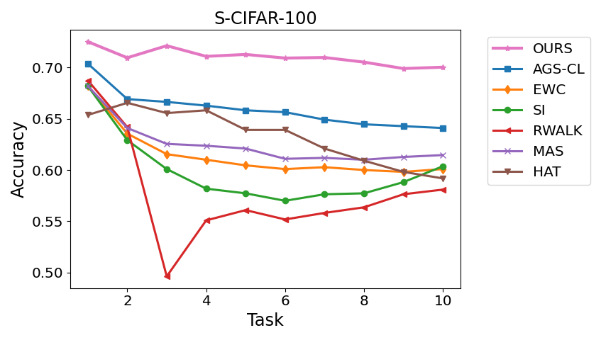
Figure 1: Average accuracy results on CIFAR-100 (10 tasks)

Models. As is common in related work (Titsias et al., 2020; Kirkpatrick et al., 2017; Nguyen et al., 2017; Pan et al., 2021; Jung et al., 2020), we evaluate RMNs on five benchmarks: Permuted-MNIST (Kirkpatrick et al., 2017)(P-MNIST), Split-MNIST(S-MNIST), Sequential Omniglot(S-OMNIGLOT) (Schwarz et al., 2018), 10 task Split-Cifar100 (Zenke et al., 2017)(S-CIFAR100) and 20 task Split-Cifar100 (RES-CIFAR). To validate the efficacy of RMNs on complex architectures, the RES-CIFAR model is trained on a Resnet18. For 10 task S-Cifar100, we used 6 convolution layers followed by 2 fully connected layers (with ReLU activations). S-MNIST, P-MNIST and S-Omniglot architectures are same as in (Titsias et al., 2020).

Results and Discussion As seen in Table 1, our RMNs set the new state of the art across all continual learning benchmarks presented, with improvements of $2.8\%$ (P-MNIST), $0.5\%$ (S-MNIST), $3.9\%$ (S-Omnliglot), $8.7\%$ (S-Cifar100) and $13.9\%$ (RES-CIFAR) over the previous SOTA. RMNs show their versatility in both simple (MLP) and complex (ResNet) architectures over both long (S-Omniglot, RES-CIFAR) and short continual learning, demonstrating their versatility. Figure 1 shows an example of the effectiveness of RMNs as compared to other methods when dealing with CF.

To keep comparisons fair amongst methods, Table 1 is divided into two parts by a 2-line separator. The above part includes all the methods which do not obey the conditions of a strict CL framework. Some compared methods(Nguyen et al., 2017; Titsias et al., 2020; Chaudhry et al., 2018; Guo et al., 2020; Pan et al., 2021) employ data replay buffers while others cannot work efficiently without one or more multi-headed layers (Nguyen et al., 2017; Chaudhry et al., 2018; Jung et al., 2020) or a version of it - for e.g. (Serr et al., 2018) use manual hard coding of layers per task. The lower part of Table 1 consists of methods which are implemented in a strict sequential learning setup. Unlike most of the compared methods, RMNs do not require any replay buffers, ensemble networks, meta networks, multi-headed layers or pretrained models and yet are able to outperform methods which do use such methods. We also compare RMNs with similar methods as mentioned in Section 2 and see that RMNs substantially outperforms every one of them as seen in Table 1.

5.2 Unsupervised CL (Testing Catastrophic Remembering)

Measuring Catastrophic Remembering For a good measure of CR, we need to evaluate how well a sequentially trained ANN discriminates between old and new data as well as how well does it discriminate between all the tasks/data after it has been trained on all of them. To that end, we propose two tests: (1) (Unsupervised) New Task/Data Detection and (2) Unsupervised Task Inference. In the new task detection setup, the ANN is given no supervision with respect to the new data or task and has to detect this change. The model’s performance (for e.g., the accuracy for each task in case of classification) is compared with the supervised continual learning version. In the second test, a trained model has to detect which specific task does the test input data belongs to. A point to be noted is that the preconditions of the sequential training paradigm mentioned in Section 1 are to be strictly observed. The tests are mutually inclusive in terms of representing effectiveness w.r.t CR alleviation i.e. a method should perform well on both tasks to be good candidate for fixing Catastrophic Remembering (while still being able to alleviate Catastrophic Forgetting).

5.2.1 New Task/Data Detection

Setup. The model is given no information about the tasks during training (and inference) time. The results are then compared with the full supervised version (Table 1). The performance degradation from the supervised learning results allow us to evaluate how well the model can alleviate CR. Here, we assume that no information of task labels is given, including the number of disparate tasks.

RMN Methodology. In this case, we initialize $f$ with only a single $\mathbb{M_{P}}$, i.e. only a single forward inference path can be learned at initialization, as seen in Line 2 of Algorithm 2 (Suppl. Sec. 2). We set the current task indicator as $est_{j}{=}0$. Then, for each minibatch $x$ encountered, we run a task-switch-detection $(TSD)$ method, denoted as $TSD(x)$ which returns a boolean value. If $TSD(x)$ returns True, then $est_{j}$ is incremented and another set of $\mathbb{M_{P}}$ is added to $f$. We use a Relevance modified Welsh’s t-test on the KL divergence between prior and posterior distributions of the model to determine a task switch (Titsias et al., 2020; Hendrycks & Gimpel, 2016; Lee et al., 2018).

Results and Discussion. Few methods (Titsias et al., 2020; Lee et al., 2020; Pan et al., 2021) have tried to effectively deal with the harder problem of learning continually without task labels and none of these follow a strict CL framework. (Titsias et al., 2020) and (Pan et al., 2021) both employ a data replay buffer whereas (Lee et al., 2020) uses generative replay and a mixture of expert models (which leads to a large increase in computational and memory requirements).

Table 2: Continual Learning without Task Labels.

Algorithm	P-MNIST	S-MNIST	S-Omniglot
FRCL$\mathcal{R}$	$94.3\pm 0.2$	$97.8\pm 0.7$	$81.47\pm 1.6$
FROMP$\mathcal{R}$	$94.9\pm 0.1$	$99.0\pm 0.1$	$-$
CN-DPM$\mathbb{C},\mathcal{R}$	$-$	$97.53\pm 0.3$	$-$
RMN (Ours)	$97.73\pm 0.1$	$99.5\pm 0.2$	$85.33\pm 1.7$

• (Lee et al., 2020)

• uses data replay buffer

The usual methodology that is followed in an Unsupervised CL learning setup involves boundary detection between current and new tasks. Table 2 shows the results of this setup amongst all the relevant methods. RMNs achieve the state of the art for Unsupervised CL Learning without the usage of data replay buffer, mixture of expert models or any kind of generative replay, unlike (Titsias et al., 2020; Pan et al., 2021; Lee et al., 2020). Ordinarily, these task detection methods employ statistical tests like Welch’s T-test over clean batches of data (the entire batch data belongs to either the current or the next task). This methodology fails when the incoming previous and the incoming batch are noisy with the incoming batch consisting of the new task data as well as old data. RMNs however can easily deal with this by filtering the incoming batch via final layer activations - only if RMNs have seen the data do they have high and confident activations before calculating the KL divergence test between the prior and posterior to detect the presence of a new set of data. However, none of the methods (Titsias et al., 2020; Lee et al., 2020) mentioned are capable of deploying over such a noisy data setup and are unable to learn continually. (Lee et al., 2020) does employ a Fuzzy Testing scenario for Split-MNIST in which there are transition phases between tasks where the amount of new data increases linearly in each batch. Comparison on the same experiment is presented in Table 3.

Table 3: Fuzzy Unsupervised Learning.

Algorithm	S-MNIST
CN-DPM$\mathbb{C},\mathcal{R}$	$93.22\pm 0.07$
RMN (Ours)	$99.1\pm 0.5$

5.2.2 Unsupervised Task Inference

Under this novel setup, the algorithm has to identify at inference time which task a data input belongs to amongst all the tasks it has learned. From a practical point of view, knowing which task in the sequential task list does the current inference data element belongs to, without human intervention opens up huge opportunities for automation and analysis.

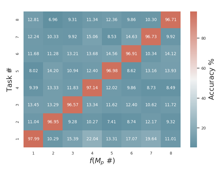
Figure 2: P-MNIST Randomized Unsupervised Task Inference

Setup. After the ANN has been trained, the test data is randomized and provided to the model for inference without its task identity (something which would happen in real world CL scenario). The model identifies the task to which the data belongs to and then the test accuracy is calculated from the correctly identified task over the entire task set. For RMNs, as task $j$ is not given at inference time, thus $max_{k}f(x,k;W)$ is returned, as seen in Algorithm 2 (Suppl. Sec. 2). Our experimental results show that for any ground-truth task label $j$, indeed the desired result is $f(x,j;W)\approx max_{k}f(x,k;W)$, which allows for unsupervised CL inference, as the pathways of different tasks don’t overlap unless the tasks are the same.

Results and Discussion. Unfortunately, we couldn’t find any SOTA CL method which can be used for this experiment, or can be used with trivial modifications. It should be possible for (Lee et al., 2020) to possibly be able to extend the method to do unsupervised task inference. However since the method employs a mixture of expert models for every task as well as generative replay which in turn rapidly drives up computational and storage memory requirements for even small ANNs, it cannot be considered a strict CL setup or even a slightly relaxed version of the same. In Figure 2, we show how our algorithm is able to detect the right task - we see that the relevance-weight combination achieves the correct maximum activation in the final layer only when the correct relevance is used. We also display the percentage of correct activations for other relevance values even if they are not maximum activations. According to our knowledge, our method is the only known continual learning method under strict CL setup constraints capable of successfully accomplishing unsupervised task inference.

6 Conclusion

In this work, we study the twin problem of catastrophic forgetting and remembering in continual learning. To resolve them, we introduce Relevance Mapping for continual learning, which applies a relevance map on the parameters of a neural network that is learned concurrently to every task. In particular, Relevance Mapping learns an optimal overlap of network parameters between sequentially learned tasks, reducing the representational overlap for dissimilar tasks, while allowing for overlap in the network parameters for related tasks. We demonstrate that our model efficiently deals with catastrophic forgetting and remembering, and achieves SOTA performance across a wide range of popular benchmarks without relaxing the conditions of a strict continual learning framework.

References

- (1) Ahn, H., Cha, S., Lee, D., and Moon, T. Uncertainty-based Continual Learning with Adaptive Regularization. pp. 11.
- Aljundi et al. (2018) Aljundi, R., Babiloni, F., Elhoseiny, M., Rohrbach, M., and Tuytelaars, T. Memory Aware Synapses: Learning What (not) to Forget. In Ferrari, V., Hebert, M., Sminchisescu, C., and Weiss, Y. (eds.), Computer Vision – ECCV 2018, volume 11207, pp. 144–161. Springer International Publishing, Cham, 2018. ISBN 978-3-030-01218-2 978-3-030-01219-9. doi: 10.1007/978-3-030-01219-9˙9. URL http://link.springer.com/10.1007/978-3-030-01219-9_9. Series Title: Lecture Notes in Computer Science.
- Ando & Zhang (2005) Ando, R. K. and Zhang, T. A framework for learning predictive structures from multiple tasks and unlabeled data. J. Mach. Learn. Res., 6:1817–1853, December 2005. ISSN 1532-4435.
- Chaudhry et al. (2018) Chaudhry, A., Dokania, P. K., Ajanthan, T., and Torr, P. H. S. Riemannian walk for incremental learning: Understanding forgetting and intransigence. In Proceedings of the European Conference on Computer Vision (ECCV), September 2018.
- Chen & Liu (2018) Chen, Z. and Liu, B. Lifelong machine learning. Synthesis Lectures on Artificial Intelligence and Machine Learning, 12(3):1–207, 2018.
- Ebrahimi et al. (2020) Ebrahimi, S., Elhoseiny, M., Darrell, T., and Rohrbach, M. Uncertainty-guided Continual Learning with Bayesian Neural Networks. April 2020. URL https://iclr.cc/virtual_2020/poster_HklUCCVKDB.html.
- Frankle & Carbin (2019) Frankle, J. and Carbin, M. The lottery ticket hypothesis: Finding sparse, trainable neural networks, 2019.
- French (1994) French, R. Dynamically constraining connectionist networks to produce distributed, orthogonal representations to reduce catastrophic interference, 1994.
- French (1991) French, R. M. Using semi-distributed representations to overcome catastrophic forgetting in connectionist networks. 1991.
- Guo et al. (2020) Guo, Y., Liu, M., Yang, T., and Rosing, T. Improved schemes for episodic memory-based lifelong learning, 2020.
- He et al. (2015) He, K., Zhang, X., Ren, S., and Sun, J. Deep residual learning for image recognition, 2015.
- Hendrycks & Gimpel (2016) Hendrycks, D. and Gimpel, K. A baseline for detecting misclassified and out-of-distribution examples in neural networks, 2016.
- Jung et al. (2020) Jung, S., Ahn, H., Cha, S., and Moon, T. Continual learning with node-importance based adaptive group sparse regularization, 2020.
- Kemker & Kanan (2017) Kemker, R. and Kanan, C. Fearnet: Brain-inspired model for incremental learning. 11 2017.
- Kemker et al. (2017) Kemker, R., McClure, M., Abitino, A., Hayes, T., and Kanan, C. Measuring catastrophic forgetting in neural networks, 2017.
- Kirkpatrick et al. (2017) Kirkpatrick, J., Pascanu, R., Rabinowitz, N., Veness, J., Desjardins, G., Rusu, A. A., Milan, K., Quan, J., Ramalho, T., Grabska-Barwinska, A., et al. Overcoming catastrophic forgetting in neural networks. Proceedings of the national academy of sciences, 114(13):3521–3526, 2017.
- Knoblauch et al. (2020) Knoblauch, J., Husain, H., and Diethe, T. Optimal Continual Learning has Perfect Memory and is NP-hard. arXiv:2006.05188 [cs, stat], June 2020. URL http://arxiv.org/abs/2006.05188. arXiv: 2006.05188.
- Koch et al. (2015) Koch, G., Zemel, R., and Salakhutdinov, R. Siamese neural networks for one-shot image recognition. In ICML deep learning workshop, volume 2. Lille, 2015.
- Krizhevsky (2012) Krizhevsky, A. Learning multiple layers of features from tiny images. University of Toronto, 05 2012.
- Kurle et al. (2020) Kurle, R., Cseke, B., Klushyn, A., Smagt, P. v. d., and Günnemann, S. Continual Learning with Bayesian Neural Networks for Non-Stationary Data. April 2020. URL https://iclr.cc/virtual_2020/poster_SJlsFpVtDB.html.
- Lake et al. (2015) Lake, B. M., Salakhutdinov, R., and Tenenbaum, J. B. Human-level concept learning through probabilistic program induction. Science, 350(6266):1332–1338, 2015. ISSN 0036-8075. doi: 10.1126/science.aab3050. URL https://science.sciencemag.org/content/350/6266/1332.
- (22) LECUN, Y. The mnist database of handwritten digits. http://yann.lecun.com/exdb/mnist/. URL https://ci.nii.ac.jp/naid/10027939599/en/.
- (23) LeCun, Y., Bengio, Y., et al. Convolutional networks for images, speech, and time series.
- Lee et al. (2020) Lee, J., Hong, H. G., Joo, D., and Kim, J. Continual Learning With Extended Kronecker-Factored Approximate Curvature. In 2020 IEEE/CVF Conference on Computer Vision and Pattern Recognition (CVPR), pp. 8998–9007, Seattle, WA, USA, June 2020. IEEE. ISBN 978-1-72817-168-5. doi: 10.1109/CVPR42600.2020.00902. URL https://ieeexplore.ieee.org/document/9157569/.
- Lee et al. (2018) Lee, K., Lee, K., Lee, H., and Shin, J. A simple unified framework for detecting out-of-distribution samples and adversarial attacks, 2018.
- Lewandowsky & Li (1995) Lewandowsky, S. and Li, S.-C. 10 - catastrophic interference in neural networks: Causes, solutions, and data. In Dempster, F. N., Brainerd, C. J., and Brainerd, C. J. (eds.), Interference and Inhibition in Cognition, pp. 329 – 361. Academic Press, San Diego, 1995. ISBN 978-0-12-208930-5. doi: https://doi.org/10.1016/B978-012208930-5/50011-8. URL http://www.sciencedirect.com/science/article/pii/B9780122089305500118.
- Li & Hoiem (2018) Li, Z. and Hoiem, D. Learning without forgetting. IEEE Transactions on Pattern Analysis and Machine Intelligence, 40(12):2935–2947, Dec 2018. ISSN 1939-3539. doi: 10.1109/tpami.2017.2773081.
- Mallya et al. (2018) Mallya, A., Davis, D., and Lazebnik, S. Piggyback: Adapting a single network to multiple tasks by learning to mask weights. In Ferrari, V., Sminchisescu, C., Weiss, Y., and Hebert, M. (eds.), Computer Vision – ECCV 2018 - 15th European Conference, 2018, Proceedings, Lecture Notes in Computer Science (including subseries Lecture Notes in Artificial Intelligence and Lecture Notes in Bioinformatics), pp. 72–88. Springer-Verlag Berlin Heidelberg, January 2018. ISBN 9783030012243. doi: 10.1007/978-3-030-01225-0˙5. 15th European Conference on Computer Vision, ECCV 2018 ; Conference date: 08-09-2018 Through 14-09-2018.
- Mermillod et al. (2013) Mermillod, M., Bugaiska, A., and BONIN, P. The stability-plasticity dilemma: investigating the continuum from catastrophic forgetting to age-limited learning effects. Frontiers in Psychology, 4:504, 2013. ISSN 1664-1078. doi: 10.3389/fpsyg.2013.00504.
- Mundt et al. (2020) Mundt, M., Hong, Y. W., Pliushch, I., and Ramesh, V. A wholistic view of continual learning with deep neural networks: Forgotten lessons and the bridge to active and open world learning, 2020.
- Nguyen et al. (2017) Nguyen, C. V., Li, Y., Bui, T. D., and Turner, R. E. Variational continual learning, 2017.
- Oswald et al. (2019) Oswald, J. v., Henning, C., Sacramento, J., and Grewe, B. F. Continual learning with hypernetworks. September 2019. URL https://openreview.net/forum?id=SJgwNerKvB.
- Pan et al. (2021) Pan, P., Swaroop, S., Immer, A., Eschenhagen, R., Turner, R. E., and Khan, M. E. Continual deep learning by functional regularisation of memorable past, 2021.
- Parisi et al. (2018) Parisi, G. I., Kemker, R., Part, J. L., Kanan, C., and Wermter, S. Continual lifelong learning with neural networks: A review, 2018.
- Robins (1993) Robins, A. Catastrophic forgetting in neural networks: the role of rehearsal mechanisms. In Proceedings 1993 The First New Zealand International Two-Stream Conference on Artificial Neural Networks and Expert Systems, pp. 65–68, Dunedin, New Zealand, 1993. IEEE Comput. Soc. Press. ISBN 978-0-8186-4260-9. doi: 10.1109/ANNES.1993.323080. URL http://ieeexplore.ieee.org/document/323080/.
- Schwarz et al. (2018) Schwarz, J., Luketina, J., Czarnecki, W. M., Grabska-Barwinska, A., Teh, Y. W., Pascanu, R., and Hadsell, R. Progress & compress: A scalable framework for continual learning. arXiv preprint arXiv:1805.06370, 2018.
- Serr et al. (2018) Serr, Suris, Miron, and Karatzoglou. Overcoming catastrophic forgetting with hard attention to the task. ArXiv, abs/1801.01423, 2018.
- Sharkey & Sharkey (1995a) Sharkey, N. and Sharkey, A. An analysis of catastrophic interference. Connect. Sci., 7:301–330, 01 1995a.
- Sharkey & Sharkey (1995b) Sharkey, N. E. and Sharkey, A. J. C. Backpropagation discrimination geometric analysis interference memory modelling neural nets. Connection Science, 7(3-4):301–330, 1995b.
- Smola et al. (2003) Smola, A., Vishwanathan, V., and Eskin, E. Laplace propagation. 01 2003.
- Srijith & Shevade (2014) Srijith, P. K. and Shevade, S. Gaussian process multi-task learning using joint feature selection. In Calders, T., Esposito, F., Hüllermeier, E., and Meo, R. (eds.), Machine Learning and Knowledge Discovery in Databases, pp. 98–113, Berlin, Heidelberg, 2014. Springer Berlin Heidelberg. ISBN 978-3-662-44845-8.
- Titsias et al. (2020) Titsias, M. K., Schwarz, J., Matthews, A. G. d. G., Pascanu, R., and Teh, Y. W. Functional Regularisation for Continual Learning with Gaussian Processes. April 2020. URL https://iclr.cc/virtual_2020/poster_HkxCzeHFDB.html.
- Yoo et al. (2020) Yoo, C., Kang, B., and Cho, M. SNOW: Subscribing to Knowledge via Channel Pooling for Transfer & Lifelong Learning of Convolutional Neural Networks. April 2020. URL https://iclr.cc/virtual_2020/poster_rJxtgJBKDr.html.
- Zenke et al. (2017) Zenke, F., Poole, B., and Ganguli, S. Continual learning through synaptic intelligence, 2017.
- Zhu & Gupta (2017) Zhu, M. and Gupta, S. To prune, or not to prune: exploring the efficacy of pruning for model compression. arXiv preprint arXiv:1710.01878, 2017.