From observations to complexity of quantum states via unsupervised learning

Abstract

The vast complexity is a daunting property of generic quantum states that poses a significant challenge for theoretical treatment, especially in non-equilibrium setups. Therefore, it is vital to recognize states which are locally less complex and thus describable with (classical) effective theories. We use unsupervised learning with autoencoder neural networks to detect the local complexity of time-evolved states by determining the minimal number of parameters needed to reproduce local observations. The latter can be used as a probe of thermalization, to assign the local complexity of density matrices in open setups and for the reconstruction of underlying Hamiltonian operators. Our approach is an ideal diagnostics tool for data obtained from (noisy) quantum simulators because it requires only practically accessible local observations.

Finding a suited notion of the complexity of quantum many-body states is a key aspect of various lines of research on correlated quantum systems. Entanglement entropy has emerged as a highly relevant information-theoretic quantity in the case of pure states, that reveals universal features in exotic states of matter Vidal et al. (2003); Calabrese and Cardy (2004); Kitaev and Preskill (2006); Fradkin and Moore (2006); Pollmann et al. (2010); Szasz et al. (2020), in quantum many-body dynamics far from equilibrium Calabrese and Cardy (2005); Bardarson et al. (2012), and it indicates the feasibility of classical computer simulations Schollwöck (2011); Orús (2014); Paeckel et al. (2019). Recently, it has also been measured experimentally using cold atoms and trapped ions Islam et al. (2015); Kokail et al. (2020). Generalizations of entanglement entropy applicable to mixed states have been proposed Plbnio and Virmani (2007) and entanglement witnesses can detect entanglement Terhal (2002), e.g., in experiments where entanglement entropy is inaccessible. An alternative perspective is that of quantum circuit complexity, which corresponds to the minimal size of a circuit to prepare the state of interest from a fiducial state Yao (1993); Dowling and Nielsen (2008); Haferkamp et al. (2021).

Entanglement and circuit complexity, however, do not universally align with the physically relevant degree of complexity of many-body states. For example, although ergodic many-body systems quickly become highly entangled under unitary non-equilibrium dynamics, the late time dynamics of physically relevant local observables is described by hydrodynamic equations of motion of a few quantities Lux et al. (2014); Bohrdt et al. (2017); Leviatan et al. (2017). Moreover, their eventual thermalization implies that a few thermodynamic quantities fully characterize local properties, and entanglement entropy turns into thermodynamic entropy of subsystems. Since typical initial states are weakly entangled, it is expected that in terms of “local complexity” associated with local observables, the non-equilibrium dynamics typically passes an “information barrier” at intermediate times. Such a “barrier” has been identified by considering the operator entanglement entropy evolution in closed and open quantum systems Dubail (2017); Wang and Zhou (2019); Noh et al. (2020); Rakovszky et al. (2020); Reid and Bertini (2021) and the envisioned time-dependence of local quantum state complexity is depicted schematically in Fig. 1.

Figure 1: Schematic picture of the “information barrier” of quantum many-body dynamics. The different shaded areas illustrate the logical structure of this paper – we address (i) infinite time steady states, (ii) practically attainable states at late but finite times, and (iii) short to intermediate times, where the “information barrier” is crossed.

This Letter introduces a novel approach to analyze the local complexity of quantum many-body states based on recently developed machine learning techniques. At the core, we employ deep autoencoder networks Hinton and Salakhutdinov (2006), which we train in an unsupervised fashion with observable expectation values, in order to obtain a dimensional reduction enabling us to assess the effective complexity of the quantum state of interest. We address different regimes of non-equilibrium dynamics of open and closed quantum systems, which are indicated in Fig. 1 by the different background shadings. The paper is structured such that we progress from (i) the infinite time limit over (ii) practically attainable steady states at late finite times to (iii) the “information barrier” itself at intermediate and short times. Following this order, we can first test our approach in a controlled setting by assigning the local complexity of thermodynamic ensembles; these are idealized local descriptions of steady states of chaotic or integrable models Rigol et al. (2007); Vidmar and Rigol (2016); Essler and Fagotti (2016). Then, we investigate the dynamical approach of a weakly dissipative system to such states in terms of our complexity measure. For nearly integrable systems, the absence of thermalization despite weak integrability breaking sources is a non-trivial effect Lange et al. (2017, 2018); Reiter et al. (2019); Lenarčič et al. (2018, 2020), which can be detected with the unsupervised learning approach. Finally, we reveal an “information barrier” at intermediate times by analyzing the time-dependent local complexity in random unitary dynamics, which has in many recent works been proven to be a useful model to analyze typical features of non-equilibrium dynamics Brown and Viola (2010); Nahum et al. (2017, 2018); von Keyserlingk et al. (2018); Rakovszky et al. (2018); Khemani et al. (2018); Chan et al. (2018a); Sünderhauf et al. (2018); Friedman et al. (2019); Chan et al. (2018b); Bertini and Piroli (2020); Reid and Bertini (2021). Besides the assertion of complexity, we demonstrate how further information about effective descriptions can be extracted, e.g., to reconstruct Hamiltonians for thermal states.

Being based on local observations, this approach is suited to exploit highly resolved observations of many-body quantum systems that are possible in modern quantum simulators Leibfried et al. (2003); Bloch et al. (2008); Islam et al. (2015); Gross and Bloch (2017); Preskill (2018); Ebadi et al. (2020); Scholl et al. (2020); Blais et al. (2020).

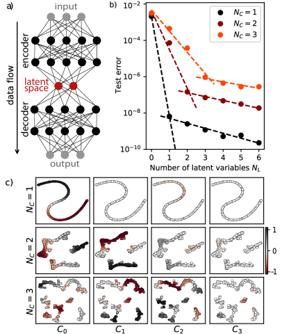
Figure 2: a) Schematic depiction of the neural autoencoder network. b) Test error as function of the number of latent variables obtained by training on the transverse-field Ising model data from (generalized) Gibbs ensembles with varying number of charges $N_{C}$. Dashed lines are linear fits included as a guide for the eye. c) t-SNE of the latent representation of (G)GEs with different number of charges $N_{C}$ and $N_{L}=4$. Color coding in each column is according to expectation values $\langle\hat{C}_{i}\rangle/N$ of charges, denoted in the bottom. Parameters: $N=12,h_{x}=0.6J,h_{z}=0$.

Autoencoder.

The autoencoder Hinton and Salakhutdinov (2006) is an artificial neural network consisting of multiple layers. The input and output layers have the same dimension, and at least one of the additional layers between the two constitutes a “bottleneck” with a considerably smaller number of $N_{L}$ neurons, spanning the $N_{L}$ dimensional latent space. The part prior to the bottleneck is called encoder, the subsequent part is the decoder; see Fig. 2a. Deep learning with autoencoder neural networks has previously been explored as a tool to investigate a variety of physical problems. Examples are unsupervised discovery of physical concepts Iten et al. (2020); Kottmann et al. (2020), the identification of entangled states Sá and Roditi (2020), encoding of quantum many-body states Luchnikov et al. (2019), or the exploration of relations to non-equilibrium statistical mechanics Zhong et al. (2020).

Here, the objective of an autoencoder is to reconstruct the input data $x$ given by local observations, despite the intermediate compression in the bottleneck. For this purpose, the reconstruction loss

$$\mathcal{L}_{\mathcal{D}_{T}}(\bm{\theta})=\frac{1}{|\mathcal{D}_{T}|}\sum_{x\in\mathcal{D}_{T}}\big{(}f_{\bm{\theta}}(x)-x\big{)}^{2}$$ (1)

over a training data set $\mathcal{D}_{T}$ is minimized by optimizing the variational parameters $\bm{\theta}$ of the neural network $f_{\bm{\theta}}$. Thereby, the encoder learns to map the input data to a suited low-dimensional latent representation, which holds the necessary information for the decoder to recover the original input $x$. Achieving a small reconstruction loss depends on the existence of such a low-dimensional representation, and too narrow bottlenecks lead to a larger loss $\mathcal{L}_{\mathcal{D}_{T}}$. Therefore, the effective dimensionality of a data set can be analyzed by varying the bottleneck width and comparing the corresponding reconstruction errors. This analysis should be conducted with validation data that was not used for training to exclude overfitting; we will call the reconstruction error (1) evaluated on the test data, the test error. Details about the network architecture and optimization are included in the Supplementary Material (SM) SM .

Training data.

In the exemplary applications below we consider quantum spin-$\frac{1}{2}$ chains, with composite Hilbert spaces $\mathcal{H}=\bigotimes_{l}h_{l}$, where $\text{dim}(h_{l})=2$ and $l$ is the lattice site index. As input for the encoder, we use data sets, where each element consists of the expectation values of all possible operator strings up to a fixed compact support $\mathcal{S}$, i.e., $O_{\rho}(\bm{\alpha})=\text{Tr}[\hat{\rho}\hat{\sigma}_{1}^{\alpha_{1}}\ldots\hat{\sigma}_{|\mathcal{S}|}^{\alpha_{|\mathcal{S}|}}]$ with density matrix $\hat{\rho}$, $\bm{\alpha}=(\alpha_{1},\ldots,\alpha_{|\mathcal{S}|})\in\{0,x,y,z\}^{|\mathcal{S}|}$ and $\hat{\sigma}_{l}^{0,x,y,z}$ denoting the identity and the Pauli matrices, respectively. Measuring these observables amounts to a full tomography of the reduced density matrix of the subsystem $\mathcal{S}$. While the corresponding cost grows exponentially with subsystem size $|\mathcal{S}|$, we show in our examples that already moderate supports $|\mathcal{S}|=3,4$ are informative of the local complexity; for larger supports it might be useful to employ the recently proposed classical shadow techniques Huang et al. (2020); Kokail et al. (2020); Elben et al. (2020).

In our analysis, we consider families of quantum states $\hat{\rho}_{\bm{\lambda}}$ parametrized by a potentially high-dimensional parameter $\bm{\lambda}$. Individual training data elements are given by observations $\{O_{\rho_{\bm{\lambda}}}(\bm{\alpha})|\bm{\alpha}\in\{0,x,y,z\}^{|\mathcal{S}|}\}$ for sampled parameters $\bm{\lambda}$. By optimizing the reconstruction objective (1) with autoencoder networks, we gain insights about the effective local complexity of $\hat{\rho}_{\bm{\lambda}}$ that is relevant for local observations. The complexity is quantified through the number of latent variables required for faithful reconstruction according to Eq. (1). For this procedure it is crucial to exhaustively sample the space of states $\hat{\rho}_{\bm{\lambda}}$ in order to avoid detecting spurious low-dimensional representations.

Idealized steady states of closed systems and Hamiltonian reconstruction.

As a first test bed, we consider (generalized) Gibbs ensembles ((G)GEs) of the spin-1/2 quantum Ising model (QIM)

$$\hat{H}=\sum_{j}\Big{(}J\hat{\sigma}_{j}^{z}\hat{\sigma}_{j+1}^{z}+h_{x}\hat{\sigma}^{x}_{j}+h_{z}\hat{\sigma}^{z}_{j}\Big{)}\ ,$$ (2)

relevant for quantum simulators Kim et al. (2011); Islam et al. (2011); Labuhn et al. (2016); Zhang et al. (2017); Ebadi et al. (2020); Scholl et al. (2020). For $h_{z}=0$, the QIM (2) is integrable, featuring an extensive set of mutually commuting local charges $\hat{C}_{i}$ (see SM SM ), one of which is the Hamiltonian Grady (1982). Conservation laws play a crucial role in the long-time description of excited integrable/chaotic systems, Fig. 1(i), when reduced density matrices become indistinguishable from GGEs/GEs of the form Rigol et al. (2007); Vidmar and Rigol (2016); Essler and Fagotti (2016)

$$\hat{\rho}_{\bm{\lambda}}=\frac{e^{\sum_{i}\lambda_{i}\hat{C}_{i}}}{\text{Tr}[e^{\sum_{i}\lambda_{i}\hat{C}_{i}}]}.$$ (3)

Although long-time states show volume law entanglement entropy Calabrese and Cardy (2005); Alba and Calabrese (2018), local observables are (for most practical purposes) determined by a few Lagrange parameters $\lambda_{i}$. Our goal is to detect these simple parametrizations.

To benchmark the utility of our approach to analyze such characteristics of long-time states, Fig. 1(i), we do not perform an actual time evolution but instead generate training data from GGEs with randomly drawn Lagrange multipliers $\lambda_{i}\in[-2,2]$ using exact diagonalization techniques for the QIM (2) at $h_{x}=0.6J$, $h_{z}=0$ with system size $N=12$. Each sampled $\bm{\lambda}$, yields a training data element with expectation values of all Pauli strings up to support $|\mathcal{S}|=3$, and we separate these samples into training and test sets, see SM SM . Fig. 2b displays the test errors, Eq. (1), achieved after training for different numbers of charges $N_{C}$ included in the GGEs. We see that the error drops rapidly with an increasing number of latent variables $N_{L}$ as long as $N_{L}<N_{C}$; for $N_{L}\geq N_{C}$ the curves level off in all cases. This behavior of the test error is expected because $N_{C}$ is the minimal number of independent variables needed for encoding the GGE data. The change of slope becomes more distinct with larger training data sets SM .

In Fig. 2c we employ t-distributed stochastic neighbor embedding (t-SNE) Van der Maaten and Hinton (2008) to visualize what the autoencoder learned to encode in its latent space. The t-SNE is a dimensional reduction technique, where the proximity of data points in the resulting low-dimensional representation is determined based on their Euclidian distance in the original space. The position of each point corresponds to the latent representation of one set of observations. The color code indicates the corresponding expectation value of the different charges. For $N_{C}=1$, we find that also for a higher-dimensional latent space, $N_{L}>N_{C}$, the latent representation of observations lies on a one-dimensional manifold with energy density monotonously changing along it. When including more charges, we see that the dimensionality of the latent representation grows. For $N_{C}>1$, the locations of extremal regions of the color code reveal that each charge can be associated with a different direction in the latent space. This indicates that the unsupervised learning procedure yielded an encoding directly related to the physical charges. In the SM SM , we show that the learned representation is connected to the charges through an invertible map, which is sufficient for an unambiguous encoding of the data.

Having demonstrated the possibility to identify and analyze ideal (G)GE states, we next turn to genuine late-time states, Fig. 1(ii). To add some additional structure to these states, we perform time evolution with respect to open quantum systems. As we show in the following, the local complexity of late-time states in closed and weakly open systems share many properties.

Steady states of open systems.

Here we characterize steady states of open systems described by the Liouville equation

$$\dot{\hat{\rho}}=i[\hat{\rho},\hat{H}]+\epsilon\sum_{j,\gamma}\big{(}\hat{L}^{(\gamma)}_{j}\hat{\rho}\hat{L}_{j}^{(\gamma)\dagger}-\frac{1}{2}\{\hat{L}_{j}^{(\gamma)\dagger}\hat{L}_{j}^{(\gamma)},\hat{\rho}\}\big{)}$$ (4)

with couplings to non-equilibrium baths represented by Lindblad operators $\hat{L}_{j}^{(\gamma)}$. The strength of the Markovian part is parametrized by $\epsilon$. In direct relation with the previous section, at a weak coupling to dissipators, $\epsilon\ll 1$, steady states for a chaotic (integrable) $\hat{H}$ can be approximated with (G)GEs, Eq. (3), which are corrected by a small $\delta\hat{\rho}(\epsilon)$, $\hat{\rho}\propto\hat{\rho}_{\bm{\lambda}}+\delta\hat{\rho}(\epsilon)$. For an integrable $\hat{H}$, the absence of thermalization despite weak integrability breaking sources is a non-trivial effect observed in weakly open systems Lange et al. (2017, 2018); Reiter et al. (2019); Lenarčič et al. (2018, 2020).

In this context, the unsupervised learning approach enables us to address several natural questions. For the integrable $\hat{H}$, we will utilize our approach to detect how many conservation laws must be considered to reproduce local observables – a question often raised in quench protocols in closed setups. For the chaotic $\hat{H}$, we will examine the effect of noise as of relevance for quantum simulators that are never completely isolated.

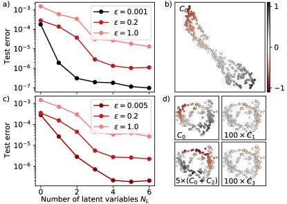
Figure 3: Results obtained by training on data from steady states for setups with different strength of openness $\epsilon$, Eq. (4), for chaotic (top) and integrable (bottom) $\hat{H}$. a,c) Test error as function of the number of latent variables. b) t-SNE of the latent representation for chaotic $\hat{H}$ and $\epsilon=0.001$, $N_{L}=5$. Color coding is with respect to energy density. d) t-SNE of the latent representation for integrable $\hat{H}$ and $\epsilon=0.005$, $N_{L}=5$. Color coding is with respect to (rescaled) densities of charges written in the inset. The gradient in the coloring with respect to $(5/N)\langle\hat{C}_{0}+\hat{C}_{2}\rangle$ is roughly perpendicular to the gradient of $\langle\hat{C}_{0}\rangle/N$. For our choice of Lindblads, inversion non-symmetric $\hat{C}_{1,3}$ show much smaller expectation values, i.e., not comparable to $\langle\hat{C}_{0}\rangle/N$ even upon rescaling with 100 and are thus not so crucial for an approximate description. Parameters: $N=40$, $h_{x}=1.152J$, $h_{z}=0.974J$ (top) and $h_{x}=1.352J$ (bottom).

The Hamiltonian $\hat{H}$ is again the QIM, Eq. (2), while the Lindblad dissipators for different data elements are randomly rotated single and two-site operators, see SM SM . The exact form of $\hat{L}_{j}^{(\gamma)}$ is not important, but sufficient randomness in either the form or the relative dissipation rates is needed to have a diverse enough training set. Fig. 3 shows results for steady states obtained using time-evolving block decimation technique Zwolak and Vidal (2004); Verstraete et al. (2004) for vectorized density matrices on systems of size $N=40$, using bond dimension $\chi=100$. For $|\mathcal{S}|=4$, we plot the test error as a function of the number of latent variables for different strengths of coupling to Markovian baths $\epsilon$ and for Hamiltonians that are either integrable or non-integrable.

At a weak coupling to baths $\epsilon=0.001$ and chaotic $\hat{H}$ the test error levels off at $N_{L}\approx 2$, Fig. 3a. In the SM SM , we show that the single latent variable, which already reaches high accuracy, again corresponds to the energy, confirming that Gibbs ensembles approximate density matrices. Further latent variables capture information about $\delta\hat{\rho}(\epsilon)$ corrections. We find that observables strongly and monotonously varying along the perpendicular direction of the tSNE representation are related to the features of the baths, i.e., the correlations that baths promote, see SM SM . This could be used for the detection of noise type, as relevant for quantum error correction.

For integrable $\hat{H}$, Fig. 3c, more than one latent variable is needed even for an approximate description. The t-SNE in Fig. 3d reveals that the first two latent variables are related to linear combinations of the two most local inversion symmetric charges $\hat{C}_{0}=\hat{H}$ and $\hat{C}_{2}$, confirming that GGEs approximately describe steady states Lange et al. (2017, 2018); Reiter et al. (2019). Furthermore, our approach exposes that of macroscopically many conservation laws, only two are particularly relevant for an approximate description of all local observables with support up to $|\mathcal{S}|=4$. Further latent variables are for corrections $\delta\hat{\rho}(\epsilon)$. At stronger $\epsilon=0.2,1.0$, a larger number of latent variables is necessary. Hence, for our choice of Lindblad operators, there is no simple emergent description.

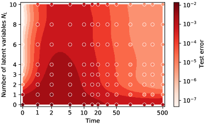
Figure 4: Complexity during random unitary evolution of $N=20$ spins captured by the autoencoder network. Starting from a simple product state, an intermediate regime of high complexity is traversed before an effective one-dimensional description emerges at late times due to the presence of a conserved charge. For times $t>1$ the scale is logarithmic. Data points (colored dots) are augmented by discretized heatmap based on a bivariate B-spline interpolation.

Random unitary evolution and information bottleneck.

Finally, we study the local complexity at intermediate times, Fig. 1(iii), by analyzing states evolved by random unitary dynamics. Random unitary circuits have recently received substantial interest because they allow the analysis of typical features of non-equilibrium dynamics Brown and Viola (2010); Nahum et al. (2017, 2018); von Keyserlingk et al. (2018); Rakovszky et al. (2018); Khemani et al. (2018); Chan et al. (2018a); Sünderhauf et al. (2018); Friedman et al. (2019); Chan et al. (2018b); Bertini and Piroli (2020); Reid and Bertini (2021). We will now show that in combination with our unsupervised learning of local complexity, they provide suited grounds to explore the information barrier, appearing at intermediate times in the time evolution from simple (product) states. To detect the information barrier, a detour away from Hamiltonian dynamics is necessary, in order to add a random component to the time evolution. From the perspective of the autoencoder, states that are obtained through deterministic dynamics starting from the few-parameter family of product states have a constant complexity: the fixed unitary map can be absorbed in the encoder/decoder of the network such that a few-parameter representation is possible at all times. On the other hand, the effective reduction of complexity at late times could also be studied under Hamiltonian dynamics when considering a higher-dimensional manifold of initial states.

Our model of random unitary evolution is based on alternating application of two-site gates on even and odd links of the spin chain. The unitary gates vary randomly from step to step, but they are homogeneous across the chain to preserve translational symmetry. Moreover, we choose the unitaries to be $U(1)$-symmetric to impose magnetization as a single conserved quantity. Building on the results of the previous sections, we anticipate that a single Lagrange multiplier associated with the magnetization conservation will locally characterize states at late times. The initial states are random translationally invariant product states. At each time step, we measure all operators with support $|\mathcal{S}|=3$ and train the autoencoder with different $N_{L}$-dimensional bottlenecks. See SM SM for details.

Fig. 4 displays the test errors that we find as a function of time and number of latent variables. The full description of the initial product state by two Bloch angles is reflected in very small test errors when using two or more latent variables. At late times a single latent variable is sufficient for faithful reconstruction, consistent with convergence to a reduced density matrix corresponding to an ensemble fully characterized by a single Lagrange multiplier. At intermediate times, however, the reconstruction error becomes large even for rather wide bottlenecks because the generic dynamics modelled by random unitary circuits generates complex quantum states, for which no effective low-dimensional parametrization exists. In that sense, our unsupervised learning approach probes the information barrier of quantum many-body dynamics. This concept of local complexity should, on the other hand, not be mistaken for the circuit complexity, which generically grows as a function of the random circuit depth Haferkamp et al. (2021).

Hamiltonian reconstruction.

When our approach reveals that data has a (near) one-dimensional latent representation (like top Fig. 2c or Fig. 3b), presumably corresponding to thermal states $\rho$, this connection can be exploited to reconstruct $\hat{H}$, as we outline now for the translationally invariant case. We first single out operators $\hat{O}(\bm{\alpha})\equiv\hat{O}_{j=1}(\bm{\alpha})=\hat{\sigma}_{1}^{\alpha_{1}}\ldots\hat{\sigma}_{|\mathcal{S}|}^{\alpha_{|\mathcal{S}|}}$ for which we measure a large average gradient of $O_{\rho}(\bm{\alpha})=\text{Tr}[\hat{\rho}\,\hat{O}(\bm{\alpha})]$ along the effective one-dimensional latent manifold, spanned by different temperatures. These are candidate Hamiltonian terms $\hat{H}=\sum_{j,\bm{\alpha}}a_{\bm{\alpha}}\hat{O}_{j}(\bm{\alpha})$. Using Newton’s method or similar, we find coefficients $a_{\bm{\alpha}}$ up to a scaling factor from the conditions $\text{Tr}[\hat{O}(\bm{\alpha})\,e^{\sum_{j,\bm{\alpha}}a_{\bm{\alpha}}\hat{O}_{j}(\bm{\alpha})}]/\text{Tr}[e^{\sum_{j,\bm{\alpha}}a_{\bm{\alpha}}\hat{O}_{j}(\bm{\alpha})}]-O_{\rho}(\bm{\alpha})=0$. Testing this approach with the data presented in Fig. 2, $h_{x}/J$ is reconstructed within the accuracy of the Newton’s method. Using the data in Fig. 3b for $\epsilon=0.001$, the relative strength of fields is obtained within 5% and 1% for $h_{x}/J$ and $h_{z}/J$, respectively. See the SM SM for more information on the algorithm. In contrast to other methods Che et al. (2020); Valenti et al. (2019); Ma et al. (2020); Xin et al. (2019), our approach is unsupervised and relies only on expectation values.

Discussion.

We have introduced an unsupervised learning approach that reveals information about the existence of effective low-dimensional descriptions of many-body quantum states. Although no domain knowledge is provided during optimization, we showed for some examples how physical information can be extracted from the trained autoencoders. In that sense, our results constitute a step towards interpretable machine learning of physics.

An alternative to our approach is the analysis of the intrinsic dimension of the data sets Wold et al. (1987); Borg and Groenen (2005); Balasubramanian et al. (2002); Van der Maaten and Hinton (2008); McInnes et al. (2018); Levina and Bickel (2004); Campadelli et al. (2015); Facco et al. (2017); Mendes-Santos et al. (2020); Lopez Tomas et al. (2018); Turkeshi (2021); Khan et al. (2021). In the SM SM we include a corresponding analysis of our data as reference. While the results are consistent, the autoencoder method seems more robust, and it has the advantage to reveal further information beyond the minimal number of independent variables.

Autoencoders could be used, for example, to detect GGEs in weakly open trapped-ions setups Reiter et al. (2019). Natural extensions of the present work could be the investigations of Floquet prethermal plateaus and of thermalization in strongly disordered many-body systems. Our method could complement the recent proposal to use supervised or confusion learning based on observations from cold atom experiments Bohrdt et al. (2020). In the SM SM , we give first evidence that autoencoders can be used for noise-type recognition, relevant for quantum error correction, which opens another exciting direction. Finally, interesting questions to explore are the possibility of learning with incomplete or imperfect observations. In that regard, refinements of the deep learning model might be required, e.g., the utilization of variational autoencoders for resilience against noise Kingma and Welling (2019).