Soliton solutions and gravitational solitons: an overview

Abstract

In this work we intend to discuss the solitonic solutions of Einstein’s field equations in vacuum by constructing the solution to $N$ solitons and studying some aspects of it. In conclusion, it will be shown how the Kerr black hole can be interpreted as a soliton solution in the case of axial symmetry.

1 Introduction

Solitons were first observed in 1834 by the Scottish engineer John Scott Russell in the Union Canal; later, with the passage of time, the solitons were observed in other contexts such as, for example, in oceanography. By soliton we mean a particular wave-like solution of non-linear differential equations in which the dispersion effect is exactly balanced by the non-linearity effects; as we will see, an important characteristic of solitonic solutions is that in their interaction they re-emerge unchanged except for a phase shift. With the intensification of research in the field of non-linear mathematical physics and on the theory of solitons, it has been discovered that this type of solution is present in many equations of great physical interest: from fluid mechanics to non-linear optics, from physics of superconductors to lattice defects in crystals, and in many other areas of physics and beyond. In fluid mechanics, the Korteweg-de Vries (KdV) equation describes long surface waves in the one-dimensional approximation and it admits soliton solutions. In the context of non-linear optics the non-linear Schroedinger equation (NLS) derives from the Helmholtz equation once it is assumed that the variation of the refractive index of the material is small compared to the refractive index itself, that it depends only by the intensity of the light and that there is paraxiality. The NLS admits solutions of solitonic character. In superconductor physics and crystallography, the sine-Gordon equation describes the dynamics, respectively, of the quantized magnetic flux in a Josephson junction and of crystal dislocations; also the sine-Gordon equation has soliton like solutions.
The main method for the search for solitonic solutions, the spectral transform, will be discussed in section 2 together with the Darboux transform, another important mathematical tool of the soliton theory that allows us to build solitonic solutions knowing a particular solution of our problem. These tools will then be applied briefly to the case of the KdV showing, in this specific case, some general considerations made in paragraph 2.1. We will mainly refer to the bibliographic references 7 ,4 and 11 .
In this paper we will mainly focus on the solitons that emerge from Einstein’s field equations in vacuum. In section 3 we will discuss the generalization of the spectral transform to the theory of gravitation and, in addition to constructing the solution to $N$ solitons and studying some properties of gravitational solitons, it will be shown how the Kerr black hole can be interpreted as a gravitational double soliton solution.

1.0.1 Notations

This conventions are adopted:

• derivatives are indicated with commas, for example $f_{i,z,z}=\partial_{z}^{2}f_{i}=\frac{\partial^{2}f_{i}}{\partial z^{2}}$;

• identity matrix will be indicated as $\mathcal{I}$;

• traces are indicated with a capital letter, for example $R=Tr(\hat{R})=Tr(R_{\alpha\beta})$;

• The commutator is denoted as $[\cdot,\cdot]$;

• The indices $i,j,h$ are to be considered added if repeated.

2 Nonlinear equations and soliton solutions

As already anticipated in the introduction, many nonlinear equations of physical interest show soliton solutions. Therefore, let us concentrate on solving nonlinear equations; the methods we will develop are the spectral transform and the Darboux transform, which will be discussed in their general features and applied to the specific case of KdV. In the first paragraph we will mainly refer 11 ,4 and 7 .

2.1 Spectral transform and Darboux transform

The spectral transform (TS) method was introduced in 1967 by Gardner, Greene, Miura and Kruskal 2 to solve the problem at the initial values of the KdV and then extended to other situations of interest, for example as did Zakharov and Shabat in 1972 8 with the NLS. The method is based on the possibility of writing the equation under consideration as a condition of integrability of an associated matrix system of two linear differential equations, the so-called the Lax pair of the problem. This has the form

$$\boldsymbol{\psi}_{,z}=\hat{U}\boldsymbol{\psi},$$ (1)

$$\boldsymbol{\psi}_{,t}=\hat{V}\boldsymbol{\psi},$$

where $\boldsymbol{\psi}$, $\hat{U}$ and $\hat{V}$ depend on a parameter, $\lambda$, called the spectral parameter and on the variables $z$ and $t$. The spectral parameter satisfies the isospectrality condition $\lambda_{,t}=0$. The condition of integrability is obtained as

$$\boldsymbol{\psi}_{,t,z}=\boldsymbol{\psi}_{,z,t}\Rightarrow\hat{V}_{,z}\boldsymbol{\psi}+\hat{V}\boldsymbol{\psi}_{,z}=\hat{U}_{,t}\boldsymbol{\psi}+\hat{U}\boldsymbol{\psi}_{,t}\Rightarrow\hat{V}_{,z}\boldsymbol{\psi}+\hat{V}\hat{U}\boldsymbol{\psi}=\hat{U}_{,t}\boldsymbol{\psi}+\hat{U}\hat{V}\boldsymbol{\psi},$$

from which follows the operatorial equation

$$\hat{V}_{,z}+\hat{V}\hat{U}-\hat{U}_{,t}-\hat{U}\hat{V}=0\Rightarrow\hat{V}_{,z}-\hat{U}_{,t}+[\hat{V},\hat{U}]=0,$$ (2)

said the Lax equation corresponding to the original equation of our Cauchy problem. Imagine that our nonlinear differential equation determines the quantity $u(z,t)$ and that the initial condition $u(z,0)$ is given. Once the appropriate Lax pair has been determined, the problem is divided into two parts: the direct problem and the inverse problem. The direct problem consists in associating the spectral parameters, such as the transmission coefficient $T(\lambda)$, the reflection coefficient $R(\lambda)$ and the elements $\lambda_{n}$ of the discrete spectrum, which correspond to the potential $u(z,0)$; these spectral parameters are denoted, as a whole, with $S(\lambda,0)$. The inverse problem, on the other hand, consists in reconstructing the potential at a generic time, $u(z,t)$, given the spectral parameters at time $t$, obtained by solving the spectral problem given by the Lax pair. The evolved spectral parameters are indicated with $S(\lambda,t)$. In summary, the idea is therefore not to find the solution $u(z,t)$ directly from the starting equation because this evolution is often too complicated, therefore it is preferable to solve the associated spectral problem, which gives us the evolution over time of the spectral parameters and from the evolved spectral parameters we can obtain the solution $u(z,t)$. The fact that it is preferable derives from the linearity of the problem when looking at it from the point of view of the spectral problem; in fact, the evolution of the spectral parameters is ultimately given by the Lax pair, which is a matrix but linear differential system. The TS method is shown in the diagram below in Figure 3.
From Figure 3 we note a certain degree of analogy with the Fourier transform scheme: in fact, the spectral transform method can be considered as a generalization to non-linear equations of the Fourier method for linear equations, and it reduces to this in the small field limit, $|u(z,t)|<<1$, and purely continuous spectrum.

$$\ \ \ \ \ \ \ \ \ \ \ \ \ \ \ \ \ \ \ \ \ \ \ \ \ u(z,0)\xrightarrow{direct\ problem}S(\lambda,0)$$ (3)

$$non\ linear\ evolution\Bigg{\downarrow}\ \ \ \ \ \ \ \ \ \ \ \ \ \ \ \ \ \ \ \ \ \ \ \ \Bigg{\downarrow}\ linear\ evolution$$

$$\ \ \ \ \ \ \ \ \ \ \ \ \ \ \ \ \ \ \ \ \ \ \ \ \ u(z,t)\xrightarrow{inverse\ problem}S(\lambda,t)$$

We are interested in solitonic solutions, which emerge in the presence of a potential $u(z,0)$ corresponding to $R(\lambda)=0$; in this case the inverse problem is considerably simplified since we pass from having to solve an integral equation to an algebraic system. The TS method shows us how solitons are intimately related to the discrete elements $\lambda_{n}$ of the spectrum: for each of them a soliton emerges; moreover each $\lambda_{n}$ is a pole of the transmission coefficient and this implies that there are as many solitons as there are poles of $T(\lambda)$.

We now introduce another instrument of particular importance: the Darboux transform (TD). First, it is important to underline that TD is an algebraic method; it consists in constructing exact solutions for a non-linear integrable equation, Starting from the knowledge of a simple exact solution called background solution, that is

$$\boldsymbol{\psi}=\hat{\chi}\boldsymbol{\psi}_{b};$$ (4)

the $\hat{\chi}$ matrix is called the dressing matrix. Assuming a dressing matrix of the shape

$$\hat{\chi}=\mathcal{I}+\sum_{k=1}^{N}\frac{\hat{O}_{k}}{\lambda-\lambda_{k}}$$ (5)

in which the $\hat{O}$ operator does not depend on the spectral parameter, the $N$ solitons solution is constructed: a $N$ poles dressing matrix can generate the $N$ solitons solution.
The TD and the TS are linked by the fact that, as will be explicitly seen in the case of the KdV, the TD adds a pole to the transmission coefficient and this involves the addition of a soliton.

2.2 The KdV case

In the previous paragraph the general lines of the spectral transform and the Darboux transform were outlined; in this paragraph we want to briefly discuss an important example: the KdV. First of all, it should be emphasized that the KdV is a model equation, together with the Hopf, Burgers equation and the NLS, of the non-linear mathematical physics; indeed these equations can be found by applying multiscale expansion to rather general classes of nonlinear PDEs; with reference to 4 , the case of the KdV is reported in appendix A.

2.2.1 Soliton $N$ solution with the spectral transform for the KdV

Let us consider the case of the KdV, which is generally written as

$$u_{,t}-6uu_{,z}+u_{,z,z,z}=0$$ (6)

with $u$ a function of $z$ and $t$, and we apply the TS to derive the one soliton solution. The Lax pair for the KdV can be written as

$$\hat{L}\psi=(-\partial_{z}^{2}+u)\psi=E\psi,$$ (7)

$$\psi_{,t}=\hat{M}\psi=(-4\partial_{z}^{3}+6u\partial_{z}+3u_{,z}+c(E))\psi,$$

where $c(E)_{,z}=0$; the integrability condition for the 7 problem returns exactly the 6 and moreover it is verified if and only if there is the isospectrality of the problem, that is $E_{,t}=0$:

$$(\hat{L}\psi)_{,t}=\hat{L}_{,t}\psi+\hat{L}\psi_{,t}=(\hat{L}_{,t}+\hat{L}\hat{M})\psi=(E\psi)_{,t}=E_{,t}\psi+E\psi_{,t}=$$ (8)

$$=E_{,t}\psi+E\hat{M}\psi=(E_{,t}+\hat{M}\hat{L})\psi\Rightarrow E_{,t}+\hat{M}\hat{L}=\hat{L}_{,t}+\hat{L}\hat{M}\Rightarrow$$

$$\Rightarrow E_{,t}=0\Leftrightarrow\hat{L}_{,t}+[\hat{L},\hat{M}]=0.$$

As can be seen from the 7 the spectral problem is that associated with the Schroedinger equation; the direct problem therefore consists in associating the spectral parameters given by the Schroedinger equation with potential $u(z,0)$. The evolution of the spectral data is always obtained from the 7 system: taking the derivative with respect to $z$ of the first equation we have

$$-\partial_{z}^{3}\psi+u_{,z}\psi+u\psi_{,z}=E\psi_{,z}\Rightarrow\psi_{,z,z,z}=u_{,z}\psi+(u-E)\psi_{,z},$$

which substituted in the second equation returns

$$\psi_{,t}=-4u_{,z}\psi-4(u-E)\psi_{,z}+6u\psi_{,z}+3u_{,z}\psi+c(E)\psi\Rightarrow$$ (9)

$$\Rightarrow\psi_{,t}=(-u_{,z}+c(E))\psi+(2u+4E)\psi_{,z}.$$

The inverse problem instead passes through the analytic properties of the eigenfunctions. We define $E=k^{2}$; for the discrete spectrum we must have $E_{n}<0$ and therefore $k_{n}=ip_{n}$. The inverse problem gives us the solution to $N$ solitons, which is obtained from the algebraic system of $N$ equations

$$(1+e^{-2p_{n}(z-4p_{n}^{2}t-\gamma_{n})})f_{n}(z,t)+\sum_{m=1,\neq n}^{N}\frac{2p_{m}e^{-2p_{m}(z-4p_{m}^{2}t-\gamma_{m})}}{p_{m}+p_{n}}f_{m}(x,t)=1,n=1,...,N;$$ (10)

where the $f_{n}(x,t)$ are the unknowns and the $\gamma_{n}$ of the constants that depend on the spectral parameters a $t=0$, together with the

$$u(z,t)=4\partial_{z}\bigg{(}\sum_{n=1}^{N}p_{n}e^{-2p_{n}(z-4p_{n}^{2}-\gamma_{n})}f_{n}(x,t)\bigg{)}.$$ (11)

The solution of the 10 system can be found with Cramer’s method and the 11 gives us the final result in the form

$$u(z,t)=-2\partial_{z}^{2}ln(det_{N}),$$ (12)

where $det_{N}$ is the determinant of the matrix associated with the $N\times N$ system 10). For example the one soliton solution is given by

$$u(z,t)=-\frac{2p_{1}^{2}}{cosh^{2}(p_{1}(z-4p_{1}^{2}t-\gamma_{1}))}=2E_{1}sech^{2}(\sqrt{|E_{1}|}(z+4E_{1}t-\gamma_{1}));$$ (13)

the solution is therefore exponentially localized with amplitude and velocity proportional to $p_{1}^{2}$ and therefore to the eigenvalue $E_{1}$.

Starting from the 12 it is possible to show that, in the interaction between $N$ solitons, the $n$-th soliton does not change its shape but experiences a shift equal to

$$\delta x_{n}=-\frac{1}{p_{n}}\bigg{\{}\prod_{j=1}^{n-1}ln\bigg{(}\bigg{|}\frac{p_{n}+p_{j}}{p_{n}-p_{j}}\bigg{|}\bigg{)}-\prod_{j=n+1}^{N}ln\bigg{(}\bigg{|}\frac{p_{n}+p_{j}}{p_{n}-p_{j}}\bigg{|}\bigg{)}\bigg{\}}.$$ (14)

2.2.2 Solitonic solutions of KdV with Darboux transform

In this section we will show, in the specific case of KdV, that the poles of the transmission coefficient are the discrete elements of the spectrum of the associated spectral problem and that the TD acts by adding poles to the transmission coefficient and therefore solitons to the background solution.
We are looking for a TD of the form

$$\boldsymbol{\psi}=\hat{\chi}\boldsymbol{\psi}_{b},$$ (15)

con $\boldsymbol{\psi}=\binom{\psi}{\psi_{,z}}$, $\boldsymbol{\psi}_{b}=\binom{\psi_{b}}{\psi_{b,z}}$ e $\hat{\chi}=\begin{pmatrix}A&B\\ C&D\end{pmatrix}$.
By making explicit the first equation of the 15 system, deriving it twice with respect to $z$, imposing that $A$ and $B$ do not depend on $k^{2}$, passing through the Riccati equation reduced to Schroedinger equation from the transformation $A=-\frac{\phi_{,z}}{\phi}$, we obtain the Darboux transformation for the KdV

$$u(z,t)=u_{b}(z,t)-2\bigg{(}\frac{\phi_{,z}}{\phi}\bigg{)}_{,z}\ ,\ \psi(z,k,t)=\psi_{b,z}(z,k,t)-\frac{\phi_{,z}}{\phi}\psi_{b}(z,k,t),$$ (16)

where $\phi$ is the solution of the Schroedinger equation $\phi_{,z,z}=(u_{b}-k^{2})\psi$. It can be shown that by choosing the null background solution and taking the solution $\phi=c_{1}e^{p(z-4p^{2}t)}+c_{2}^{-p(z-4p^{2}t)}$ for $k=ip$, with the right choice of the constants $c_{1}$ and $c_{2}$ we get back the solution 13. We consider a generic background solution $u_{b}(z,t)$ and choose as $\psi_{b}(z,t)$ the Jost eigenfunction defined as

$$\begin{cases}J_{b}(z,k,t)\simeq e^{-ikz}&per\ z\simeq-\infty\\ J_{b}(z,k,t)\simeq a_{b}(k)e^{-ikz}+b_{b}(k)e^{ikz}&per\ z\simeq+\infty\end{cases},$$ (17)

and let $\phi$ be the corresponding solution of the Lax pair for $k=ip$ with the property that

$$\phi\simeq\alpha_{\pm}e^{-pz}+\beta_{\pm}e^{pz},\ \ per\ z\simeq\pm\infty,$$

then it follows, again for $z\simeq\pm\infty$,

$$\frac{\phi_{,z}}{\phi}=\frac{-p\alpha_{\pm}e^{-pz}+p\beta_{\pm}e^{pz}}{\alpha_{\pm}e^{-pz}+\beta_{\pm}e^{pz}}\simeq\pm p.$$ (18)

Using the 17 and 18 in the second of 16 you get a $z\simeq-\infty$

$$\psi(z,k,t)\simeq-ike^{-ikz}-pe^{-ikz}=-i(k+ip)e^{-ikz}.$$ (19)

Let $J(z,k,t)$ be the Jost eigenfunction corresponding to the potential $u(z,t)$, defined analogously to $J_{b}(z,k,t)$, that is

$$\begin{cases}J(z,k,t)\simeq e^{-ikz}&per\ z\simeq-\infty\\ J(z,k,t)\simeq a(k)e^{-ikz}+b(k)e^{ikz}&per\ z\simeq+\infty\end{cases};$$ (20)

from 19, 20, from the second of 16 and from 17 we have

$$\psi(z,k,t)\simeq-i(k+ip)J(z,k,t)\Rightarrow J(z,k,t)=\frac{1}{-i(k+ip)}\bigg{(}J_{b,z}(z,k,t)-\frac{\phi_{,z}}{\phi}J_{b}(z,k,t)\bigg{)}$$ (21)

and from this, thanks to the 17 and 18, it immediately follows that for $z\simeq\infty$

$$J(z,k,t)\simeq\frac{i}{k+ip}\bigg{(}-ik\big{(}a_{b}(k)e^{-ikz}-b_{b}(k)e^{ikz}\big{)}-p\big{(}a_{b}(k)e^{-ikz}+b_{b}(k)e^{ikz}\big{)}\bigg{)}=$$ (22)

$$=\frac{i}{k+ip}\bigg{(}a_{b}(k)e^{-ikz}\big{(}-ik-p\big{)}+b_{b}(k)e^{ikz}\big{(}ik-p\big{)}\bigg{)}=$$

$$=\frac{k-ip}{k+ip}a_{b}(k)e^{-ikz}+\frac{-k-ip}{k+ip}b_{b}(k)e^{ikz}=\frac{k-ip}{k+ip}a_{b}(k)e^{-ikz}-b_{b}(k)e^{ikz},$$

which must ultimately be the same as 20

$$a(k)=\frac{k-ip}{k+ip}a_{b}(k)\ ,\ b(k)=-b_{b}(k).$$ (23)

Since in general, the $a(k)$ and the $b(k)$ are related to the transmission and reflection coefficients by the

$$T(k)=\frac{1}{a(k)}\ ,\ R(k)=\frac{b(k)}{a(k)},$$ (24)

we conclude that

$$T(k)=\frac{k+ip}{k-ip}T_{b}(k)\ ,\ R(k)=-R_{b}(k);$$ (25)

the Darboux transform adds a pole placed in $k=ip$ to the transmission coefficient and therefore a zero to $a(k)$. We therefore consider the zero $k=ip:=k_{0}$; since $|a(k)|^{2}-|b(k)|^{2}=1$ and $a(k)$ is analytic in the upper half plane, we have $Im(k_{0})>0$ and therefore $p>0$. From the definition of the Jost function it follows that

$$\begin{cases}J(z,k_{0},t)\simeq e^{-ik_{0}z}=e^{pz}\rightarrow 0&per\ z\rightarrow-\infty\\ J(z,k_{0},t)\simeq a(k_{0})e^{-ik_{0}z}+b(k_{0})e^{ik_{0}z}=b(k_{0})e^{-pz}\rightarrow 0&per\ z\rightarrow+\infty\end{cases};$$ (26)

that is, normalizable functions which therefore correspond to discrete eigenvalues: the poles of the transmission coefficient are discrete elements of the spectrum.
The two results obtained allow us to conclude that TD adds solitons to the background solution.

3 Gravitational solitons

In this chapter we look at the soliton solutions of Einstein’s equations in vacuum: the so-called gravitational solitons. The application and extension of the TS technique to general relativity begins at the end of the 1970s thanks to the works of Belinski, Zakharov and Maison 3 ,9 ,10 and continues with the extension in the context of the Maxwell-Einstein equations by Alekseev 1 in the early 1980s.
Gravitational solitons have some interesting properties, some of these will be discussed in paragraph 3.2. In the last section, with reference 11 , we will discuss how the Kerr black hole can be interpreted as a two soliton solution of the field equations in the presence of axial symmetry.

3.1 Generalization of the spectral transform by gravitation theory and solution to $N$ solitons

Let us start by establishing the problem. Einstein field equations are written

$$E_{\mu\nu}=\frac{8\pi G}{c^{4}}T_{\mu\nu},$$ (27)

the tensor $E_{\mu\nu}$ is called the Einstein tensor and is defined as $E_{\mu\nu}:=R_{\mu\nu}-\frac{1}{2}g_{\mu\nu}R$ where $R_{\mu\nu}$ is the Ricci tensor and $T_{\mu\nu}$ is the energy-momentum tensor of the source.
The trace of the Einstein tensor returns $E=-R$ and, thanks to 27, we have $R=-\frac{8\pi G}{c^{4}}T$ and using the 27 again

$$E_{\mu\nu}=R_{\mu\nu}+\frac{1}{2}g_{\mu\nu}\frac{8\pi G}{c^{4}}T=\frac{8\pi G}{c^{4}}T_{\mu\nu}\Rightarrow R_{\mu\nu}=\frac{8\pi G}{c^{4}}\bigg{(}T_{\mu\nu}-\frac{1}{2}g_{\mu\nu}T\bigg{)};$$ (28)

in vacuum the momentum energy tensor is identically zero and the field equations can be expressed as

$$R_{\mu\nu}=0.$$ (29)

They are a system of differential equations for the 10 independent components of the metric and represent our starting problem. From here on we will use the geometric units in which $c=G=1$.

The TS method, defined in its general lines in section 2, is applicable only when the unknown function depends on two variables; in general, however, the metric depends on the three spatial coordinates and the time coordinate. We therefore assume that space-time admits two Killing vector fields of type space that allow us to eliminate the dependence on two spatial variables: $x^{1}$ and $x^{2}$. With this choice, the metric depends only on $x^{0}=t$ and $x^{3}=z$. To simplify the problem further we refer to the gauge symmetry of general relativity: symmetry under diffeomorphisms. In four-dimensional space-time this symmetry allows us to impose 4 conditions on the metric without loss of generality: we will impose that

$$g_{00}=-g_{33}\ ,\ g_{03}=0\ ,\ g_{0i}=0,$$ (30)

where $i=1,2$.
Under these hypotheses, the space-time interval is written as

$$ds^{2}=g_{\mu\nu}dx^{\mu}dx^{\nu}=g_{00}(dt^{2}-dz^{2})+g_{ij}dx^{i}dx^{j}+2g_{i3}dx^{i}dz,$$ (31)

in which, from here to the end of paragraph 3.2, $i,j=1,2$ (later on we will introduce the index $h$, which also runs on 1 and 2). It is not yet known how to apply the TS to the 31 metric: further simplification is needed. Since we have exhausted our freedom to manipulate the metric without loss of generality, we must impose as a physical condition that $g_{i3}=0$; this allows us to write

$$ds^{2}=g_{00}(dt^{2}-dz^{2})+g_{ij}dx^{i}dx^{j}.$$ (32)

We note that if we had chosen the Killing fields, one of the space like and one of the time type, we would have obtained a metric similar to 32 but stationary, in which the independent variables would be both space like; this case will be considered in paragraph 3.3 to derive the Kerr metric.

We call $\hat{g}$ the $2\times 2$ block $g_{ij}$ and set $det(\hat{g})=\alpha^{2}$; the equations 29 for the metric 32 are divided into two sets which, passing to the light cone coordinates introduced by $\zeta:=\frac{1}{2}(z+t)$ e $\eta:=\frac{1}{2}(z-t)$, take the form

$$\big{(}\alpha\hat{g}_{,\zeta}\hat{g}^{-1}\big{)}_{,\eta}+\big{(}\alpha\hat{g}_{,\eta}\hat{g}^{-1}\big{)}_{,\zeta}=0;$$ (33)

$$(ln(g_{00}))_{,\zeta}(ln(\alpha))_{,\zeta}=(ln(\alpha))_{,\zeta,\zeta}+\frac{A^{2}}{4\alpha^{2}}\ ,\ (ln(g_{00}))_{,\eta}(ln(\alpha))_{,\eta}=(ln(\alpha))_{,\eta,\eta}+\frac{B^{2}}{4\alpha^{2}},$$

where $\hat{A}:=-\alpha\hat{g}_{,\zeta}\hat{g}^{-1}$ and $\hat{B}:=\alpha\hat{g}_{,\eta}\hat{g}^{-1}$. The first of the equations 33 gives us the block $2\times 2$ and the second ones gives us $g_{00}$, once given $\hat{g}$. We also note that taking the trace of the first equation and making use of the fact that $det(\hat{g})=\alpha^{2}$ yields

$$\alpha_{,\zeta,\eta}=0;$$ (34)

the root of the determinant satisfies the wave equation.
The first of the 33 is a second order equation and is therefore equivalent to a system of two first order equations. These two equations can be obtained directly from the definitions of $\hat{A}$ and $\hat{B}$: for the former it is sufficient to replace the definitions in the first of the 33; the second is instead the condition of integrability between $\hat{A}$ and $\hat{B}$ with respect to $\hat{g}$, that is

$$\hat{B}_{,\zeta}-\hat{A}_{,\eta}=0;$$ (35)

$$\hat{A}_{,\eta}+\hat{B}_{,\zeta}+\alpha^{-1}[\hat{A},\hat{B}]-\alpha_{,\eta}\alpha^{-1}\hat{A}-\alpha_{,\zeta}\alpha^{-1}\hat{B}=0.$$

The 35 are just a rewrite of the 29 field equations.

The next step is the search for an appropriate Lax pair that defines the spectral problem and therefore depends on a complex parameter: the spectral parameter $\lambda$. For this purpose we define the operators

$$\hat{D}_{-}:=\partial_{\zeta}-\frac{2\alpha_{,\zeta}\lambda}{\lambda-\alpha}\partial_{\lambda}\ ,\ \hat{D}_{+}:=\partial_{\eta}+\frac{2\alpha_{,\eta}\lambda}{\lambda+\alpha}\partial_{\lambda}$$ (36)

and consider the following system of equations

$$\hat{D}_{-}\boldsymbol{\psi}=\frac{\hat{A}}{\lambda-\alpha}\boldsymbol{\psi},$$ (37)

$$\hat{D}_{+}\boldsymbol{\psi}=\frac{\hat{B}}{\lambda+\alpha}\boldsymbol{\psi},$$

where $\boldsymbol{\psi}=\boldsymbol{\psi}(\zeta,\eta,\lambda)$ is called generating matrix; for $\lambda=0$ the system reduces to

$$\boldsymbol{\psi}_{,\zeta}(\zeta,\eta,0)=-\frac{\hat{A}}{\alpha}\boldsymbol{\psi}(\zeta,\eta,0)\Rightarrow\hat{A}=-\alpha\boldsymbol{\psi}_{,\zeta}(\zeta,\eta,0)\boldsymbol{\psi}^{-1}(\zeta,\eta,0);$$ (38)

$$\boldsymbol{\psi}_{,\eta}(\zeta,\eta,0)=\frac{\hat{B}}{\alpha}\boldsymbol{\psi}(\zeta,\eta,0)\Rightarrow\hat{B}=\alpha\boldsymbol{\psi}_{,\eta}(\zeta,\eta,0)\boldsymbol{\psi}^{-1}(\zeta,\eta,0)$$

and, compared with the definitions of $\hat{A}$ and $\hat{B}$, it allows us to conclude that the block $2\times 2$ is nothing more than the generating matrix evaluated for $\lambda=0$:

$$\hat{g}(\zeta,\eta)=\boldsymbol{\psi}(\zeta,\eta,0).$$ (39)

We know that for the integration procedure it is necessary to know a backgound solution $\hat{g}_{b}$ from which, thanks to the definitions of $\hat{A}$ and $\hat{B}$ we get the $\hat{A}_{b}$ and $\hat{B}_{b}$ matrices which we replace in the system 37 allow us to get the background generating matrix $\boldsymbol{\psi}_{b}$. We therefore operate a Darboux transform of the form

$$\boldsymbol{\psi}=\hat{\chi}\boldsymbol{\psi}_{b}$$ (40)

which replaced in the system 37 returns a system of equations for the dressing matrix

$$\hat{D}_{-}\hat{\chi}=\frac{(\hat{A}\hat{\chi}-\hat{\chi}\hat{A_{b}})}{\lambda-\alpha};$$ (41)

$$\hat{D}_{+}\hat{\chi}=\frac{(\hat{B}\hat{\chi}-\hat{\chi}\hat{B_{b}})}{\lambda+\alpha}.$$

Putting together 39 and 40 we see that

$$\hat{g}(\zeta,\eta)=\boldsymbol{\psi}(\zeta,\eta,0)=\hat{\chi}(\zeta,\eta,0)\boldsymbol{\psi}_{b}(\zeta,\eta,0)=\hat{\chi}(\zeta,\eta,0)\hat{g}_{b}(\zeta,\eta);$$ (42)

at this point it is important to remember that the metric is real and symmetric; this implies having to impose conditions for the dressing matrix and the generating matrix in order to respect the properties of the metric; these conditions are expressed as

$$\hat{\chi}^{*}(\zeta,\eta,\lambda^{*})=\hat{\chi}(\zeta,\eta,\lambda)\ ,\ \boldsymbol{\psi}^{*}(\zeta,\eta,\lambda^{*})=\boldsymbol{\psi}(\zeta,\eta,\lambda)\ ,\ \hat{g}=\hat{\chi}(\zeta,\eta,\lambda)\hat{g}_{b}\hat{\chi}^{T}(\zeta,\eta,\alpha^{2}/\lambda);$$ (43)

where $*$ indicate complex conjugation. We underline that, for the moment, condition $det(\hat{g})=\alpha^{2}$ has not yet been imposed; the condition is imposed by requiring that

$$\hat{g}^{(f)}=\alpha\frac{\hat{g}}{\sqrt{det(\hat{g})}},$$ (44)

where the superscript $(f)$ underlines that this is the solution that respects all the physical properties of the metric: this is physical solution. Obviously, 44 involves a transformation of the $\hat{A}$ and $\hat{B}$ matrices which results in new equations for the $g_{00}$ component which will return the physical component, $g_{00}^{(f)}$.

We then proceed by discussing the construction of the $N$ solitons solution. This solution emerges by imposing a rational dependence of the dressing matrix on the spectral parameter with a finite number of simple poles

$$\hat{\chi}=\mathcal{I}+\sum_{k=1}^{N}\frac{\hat{O}_{k}}{\lambda-\lambda_{k}},$$ (45)

where $\hat{O}_{k}$ does not depend on the spectral parameter; from the reality condition of the matrix $\hat{g}$, and therefore from the first of the 43, it follows that the poles are either real or appear as pairs of conjugate complexes. The final solution is given by the 42 so

$$\hat{g}(\zeta,\eta)=\bigg{(}\mathcal{I}-\sum_{k=1}^{N}\frac{\hat{O}_{k}}{\lambda_{k}}\bigg{)}\hat{g}_{b}(\zeta,\eta);$$ (46)

it remains therefore to determine the matrix $\hat{O}_{k}$. For this purpose, we plug 45 in system 41 and the equations must be satisfied at the pole; these equations gives us important information.
The first is obtained by noting that the operators $\hat{D_{-}}$ and $\hat{D_{+}}$ contain derivations with respect to $\zeta$, $\eta$ and $\lambda$ and that, when applied to the non-trivial part of the dressing matrix, they produce terms containing double poles, terms that are not present in the second member: it is necessary that the coefficients of the double poles cancel out. In fact, studying only the $k$-th term for linearity we have

$$\bigg{(}\partial_{\zeta}-\frac{2\alpha_{,\zeta}\lambda}{\lambda-\alpha}\partial_{\lambda}\bigg{)}\frac{\hat{O}_{k}}{\lambda-\lambda_{k}}=\frac{\hat{O}_{k,\zeta}}{\lambda-\lambda_{k}}+\hat{O}_{k}\bigg{(}\frac{-\lambda_{,\zeta}}{(\lambda-\lambda_{k})^{2}}\bigg{)}-\frac{2\alpha_{,\zeta}\lambda}{\lambda-\alpha}\frac{\hat{O}_{k}}{(\lambda-\lambda_{k})^{2}};$$ (47)

$$\bigg{(}\partial_{\eta}+\frac{2\alpha_{,\eta}\lambda}{\lambda+\alpha}\partial_{\lambda}\bigg{)}\frac{\hat{O}_{k}}{\lambda-\lambda_{k}}=\frac{\hat{O}_{k,\eta}}{\lambda-\lambda_{k}}+\hat{O}_{k}\bigg{(}\frac{-\lambda_{,\eta}}{(\lambda-\lambda_{k})^{2}}\bigg{)}+\frac{2\alpha_{,\eta}\lambda}{\lambda+\alpha}\frac{\hat{O}_{k}}{(\lambda-\lambda_{k})^{2}};$$

eliminating coefficients of the double poles calculated on the poles we have

$$\bigg{(}-\lambda_{,\zeta}-\frac{2\alpha_{,\zeta}\lambda}{\lambda-\alpha}\bigg{)}\bigg{|}_{\lambda=\lambda_{k}}=0\Rightarrow\lambda_{k,\zeta}=\frac{2\alpha_{,\zeta}\lambda_{k}}{\alpha-\lambda_{k}};$$ (48)

$$\bigg{(}-\lambda_{,\eta}+\frac{2\alpha_{,\eta}\lambda}{\lambda+\alpha}\bigg{)}\bigg{|}_{\lambda=\lambda_{k}}=0\Rightarrow\lambda_{k,\eta}=\frac{2\alpha_{,\eta}\lambda_{k}}{\alpha+\lambda_{k}};$$

the 48 determine the trajectories of the poles: the poles are not fixed but move in space-time. Moreover, noting that $\hat{O}_{k}$ and $\hat{\chi}^{-1}(\lambda_{k})$ are degenerate matrices , then we can write them as

$$(\hat{O}_{k})_{ij}=n^{(k)}_{i}m^{(k)}_{j}\ ,\ (\hat{\chi}^{-1}_{k}(\lambda_{k}))_{ij}=q^{(k)}_{i}p^{(k)}_{j};$$ (49)

we rewrite the equations 41 by multiplying them from the right by $\hat{\chi}^{-1}$

$$\frac{\hat{A}}{\lambda-\alpha}=(\hat{D}_{-}\hat{\chi})\hat{\chi}^{-1}+\hat{\chi}\frac{\hat{A}_{b}}{\lambda-\alpha}\hat{\chi}^{-1},$$ (50)

$$\frac{\hat{B}}{\lambda+\alpha}=(\hat{D}_{+}\hat{\chi})\hat{\chi}^{-1}+\hat{\chi}\frac{\hat{B}_{b}}{\lambda+\alpha}\hat{\chi}^{-1};$$

since the left sides of the equations 50 are regular to the poles $\lambda=\lambda_{k}$, it follows that the residues of the poles in the second members must be zero, which leads to the equations

$$\hat{O}_{k,\zeta}\hat{\chi}^{-1}(\lambda_{k})+\hat{O}_{k}\frac{\hat{A}_{b}}{\lambda_{k}-\alpha}\hat{\chi}^{-1}(\lambda_{k})=0,$$ (51)

$$\hat{O}_{k,\eta}\hat{\chi}^{-1}(\lambda_{k})+\hat{O}_{k}\frac{\hat{B}_{b}}{\lambda_{k}+\alpha}\hat{\chi}^{-1}(\lambda_{k})=0.$$

Inserting the 49 into the 51 equations we obtain the equations that determine the vectors $m_{i}^{(k)}$:

$$\bigg{(}m^{(k)}_{i,\zeta}+m_{j}^{(k)}\frac{(\hat{A}_{b})_{ij}}{\lambda_{k}-\alpha}\bigg{)}q_{i}^{(k)}=0,$$ (52)

$$\bigg{(}m^{(k)}_{i,\eta}+m_{j}^{(k)}\frac{(\hat{B}_{b})_{ij}}{\lambda_{k}+\alpha}\bigg{)}q_{i}^{(k)}=0,$$

whose solution is given by

$$m_{i}^{(k)}=m_{0j}^{(k)}(\boldsymbol{\psi}_{b}^{-1}(\lambda_{k},\zeta,\eta))_{ji}$$ (53)

where the $m_{0j}^{(k)}$ are arbitrary complex constant vectors. To determine the $n_{i}^{(k)}$ the third condition of 43 is exploited, which allows, ultimately, to write the vectors $n_{i}^{(k)}$ as

$$n_{i}^{(k)}=\sum_{l=1}^{N}\frac{1}{\lambda_{l}}(\hat{\Pi})_{kl}L_{i}^{(l)},$$ (54)

where $L_{i}^{(l)}:=m_{j}^{(l)}(\hat{g}_{b})_{ji}$ and $(\hat{\Pi})_{kl}:=(\hat{\Gamma}^{-1})_{kl}$ with $(\hat{\Gamma})_{kl}:=-m_{i}^{(k)}m_{j}^{(l)}(\hat{g}_{b})_{ij}(\alpha^{2}-\lambda_{k}\lambda_{l})^{-1}$.

From 46, using the first of the 49 and 54 gives

$$(\hat{g})_{ij}=(\hat{g}_{b})_{ij}-\sum_{k=1}^{N}\frac{(\hat{O}_{k})_{ih}}{\lambda_{k}}(\hat{g}_{b})_{hj}=(\hat{g}_{b})_{ij}-\sum_{k=1}^{N}\frac{1}{\lambda_{k}}n_{i}^{(k)}m_{h}^{(k)}(\hat{g}_{b})_{hj}=$$ (55)

$$=(\hat{g}_{b})_{ij}-\sum_{k=1}^{N}\sum_{l=1}^{N}\frac{1}{\lambda_{k}}\frac{1}{\lambda_{l}}(\hat{\Pi})_{kl}L_{i}^{(l)}\underbrace{m_{h}^{(k)}(\hat{g}_{b})_{hj}}_{=L_{j}^{(k)}}=(\hat{g}_{b})_{ij}-\sum_{k=1}^{N}\sum_{l=1}^{N}\frac{1}{\lambda_{k}}\frac{1}{\lambda_{l}}(\hat{\Pi})_{kl}L_{i}^{(l)}L_{j}^{(k)};$$

it should be stressed, however, that the solution 55 is not the physical one: condition $det(\hat{g})=\alpha^{2}$ is not satisfied. To obtain the physical solution we refer to 44; the computation of the determinant of $\hat{g}$ can be performed step by step: it is first computed for the one soliton solution, then the physical soliton solution is used as the background solution and the two soliton solution is constructed , the determinant is computed and the two soliton solution is used as the backgound solution to add another soliton, the determinant is computed and so on. As already mentioned, the calculation of the solution $\hat{g}^{(f)}$ implies that the coefficient $g_{00}$ must also be recalculated to obtain the physical coefficient $g_{00}^{(f)}$. In conclusion we get

$$\hat{g}^{(f)}=\frac{\hat{g}}{\alpha^{N}}\prod_{k=1}^{N}\lambda_{k};$$ (56)

$$g_{00}^{(f)}=Cg_{b00}\alpha^{-\frac{N^{2}}{2}}\bigg{(}\prod_{k=1}^{N}\lambda_{k}\bigg{)}^{N+1}\bigg{(}\prod_{k>l=1}^{N}\frac{1}{(\lambda_{k}-\lambda_{l})^{2}}\bigg{)}det(\hat{\Gamma});$$

where $C$ is an arbitrary constant to choose with appropriate sign in order to have the correct sign for $g^{(f)}_{00}$; $g_{b00}$ is the $g_{00}$ background solution corresponding to $\hat{g}_{b}$; $\hat{g}$ is provided by 55.

The solution to $N$ solitons is therefore given by replacing the 56 in the space-time interval 32 and remembering the 55

$$ds^{2}=g^{(f)}_{00}(dt^{2}-dz^{2})+g^{(f)}_{ij}dx^{i}dx^{j}=$$ (57)

$$=Cg_{b00}\alpha^{-\frac{N^{2}}{2}}\bigg{(}\prod_{k=1}^{N}\lambda_{k}\bigg{)}^{N+1}\bigg{(}\prod_{k>l=1}^{N}\frac{1}{(\lambda_{k}-\lambda_{l})^{2}}\bigg{)}det(\hat{\Gamma})(dt^{2}-dz^{2})+$$

$$+\frac{\big{(}(\hat{g}_{b})_{ij}-\sum_{k,l=1}^{N}\lambda_{k}^{-1}\lambda_{l}^{-1}(\hat{\Pi})_{kl}L_{i}^{(k)}L^{(l)}_{j}\big{)}}{\alpha^{N}}\bigg{(}\prod_{k=1}^{N}\lambda_{k}\bigg{)}dx^{i}dx^{j};$$

where, $L_{i}^{(l)}:=m_{j}^{(l)}(\hat{g}_{b})_{ji}$ and $(\hat{\Pi})_{kl}:=(\hat{\Gamma}^{-1})_{kl}$ with $(\hat{\Gamma})_{kl}:=-m_{i}^{(k)}m_{j}^{(l)}(\hat{g}_{b})_{ij}(\alpha^{2}-\lambda_{k}\lambda_{l})^{-1}$.

3.2 Some properties of gravitational solitons

Given built the $N$ solitons solution, we now want to discuss some interesting properties of gravitational solitons.
We explicitly report the solution to $N=1$ solitons; with reference to the 56 we have, considering that in this case $\Pi$ and $\Gamma$ are not matrices:

$$({\hat{g}}^{(f1)})_{ij}=\frac{(\hat{g}_{b})_{ij}}{\alpha}\lambda_{1}-\bigg{(}\frac{(\alpha^{2}-\lambda_{1}^{2})L_{i}L_{j}\lambda_{1}}{-\alpha\lambda_{1}^{2}m_{i}m_{j}(\hat{g}_{b})_{ij}}\bigg{)}=\frac{(\hat{g}_{b})_{ij}}{\alpha}\lambda_{1}+\bigg{(}\frac{(\alpha^{2}-\lambda_{1}^{2})L_{i}L_{j}}{\alpha\lambda_{1}m_{i}m_{j}(\hat{g}_{b})_{ij}}\bigg{)},$$ (58)

$$\hat{g}_{00}^{(f1)}=\tilde{C}g_{b00}\alpha^{-\frac{1}{2}}\lambda_{1}^{2}m_{i}m_{j}(\hat{g}_{b})_{ij}(\alpha^{2}-\lambda_{1}^{2})^{-1},$$

where the superscript $(f1)$ indicates the physical solution to a soliton. The trajectory of the pole $\lambda_{1}$ is given by the equations 48 with $k=1$; the solution of these equations is given by the roots of the quadratic equation

$$\lambda_{1}^{2}+2(\beta-w_{1})\lambda_{1}+\alpha^{2},$$ (59)

where $w_{1}$ is an arbitrary constant and $\alpha$ and $\beta$ are two independent solutions of the equation 34. The solutions of 59 are

$$\lambda_{1}^{(in)}=-(\beta-w_{1})+\sqrt{(\beta-w_{1})^{2}-\alpha^{2}}=(w_{1}-\beta)\bigg{(}1-\sqrt{1-\frac{\alpha^{2}}{(\beta-w_{1})^{2}}}\bigg{)}$$ (60)

$$\lambda_{1}^{(out)}=-(\beta-w_{1})-\sqrt{(\beta-w_{1})^{2}-\alpha^{2}}=(w_{1}-\beta)\bigg{(}1+\sqrt{1-\frac{\alpha^{2}}{(\beta-w_{1})^{2}}}\bigg{)},$$

apexes $(in)$ and $(out)$ underline that the solutions are inside or outside the circle generated by $|\lambda|=\alpha$; specifically $|\lambda_{1}^{(in)}|<\alpha$ and $|\lambda_{1}^{(out)}|>\alpha$. In the figure below we shows the case where $\lambda_{1}^{(in)}$ and $\lambda_{1}^{(out)}$ are real with $w_{1}=3$ and $\alpha=2$.

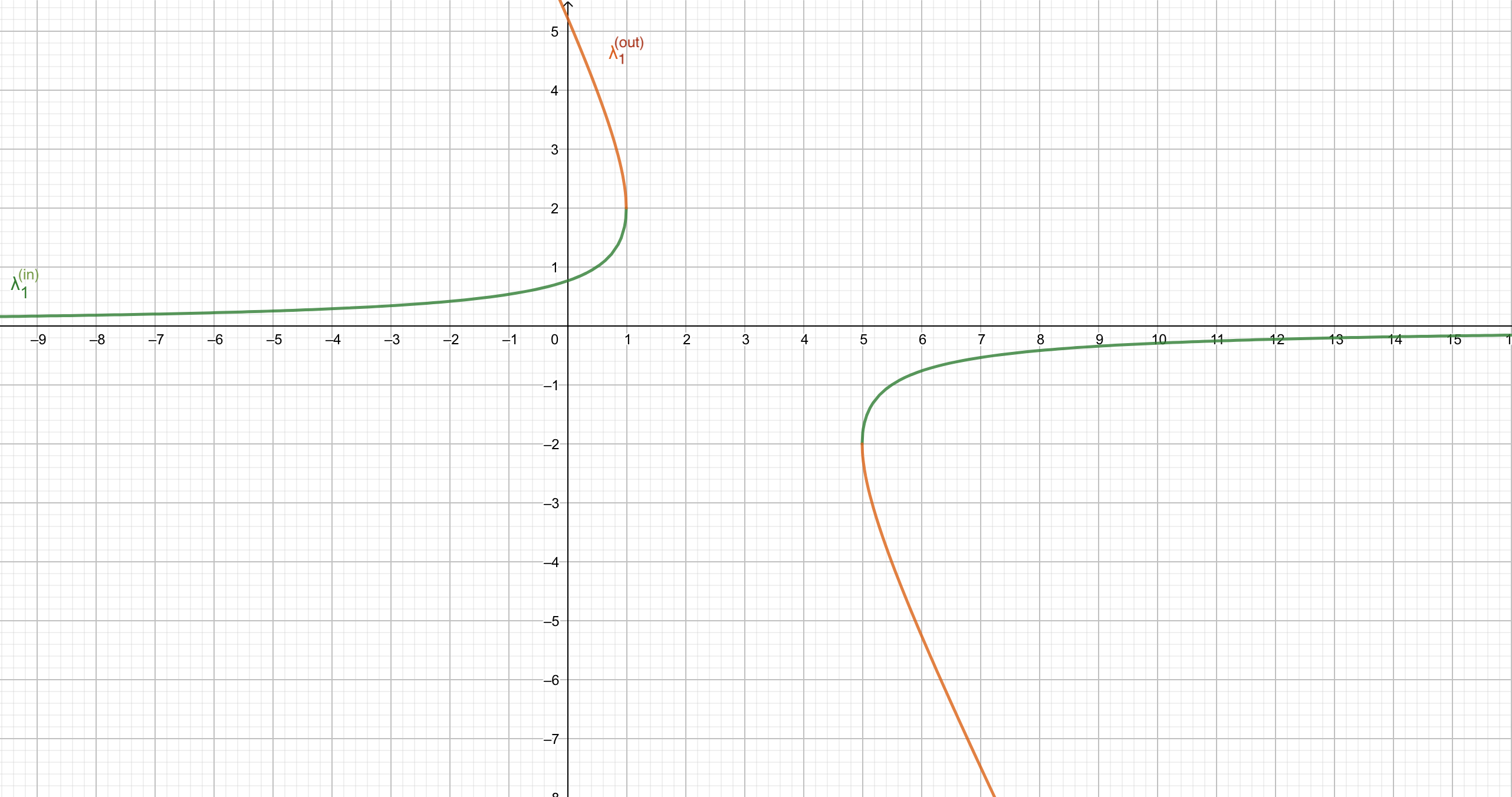
Figure 1: Andamento di $\lambda_{1}^{(in)}$ (linea verde) e $\lambda_{1}^{(out)}$ (linea arancione) in funzione di $\beta$ nel caso in cui siano reali, con $w_{1}=3$ e $\alpha=2$. Si nota che $|\lambda_{1}^{(in)}|$ è sempre minore di $\alpha=2$ mentre $|\lambda_{1}^{(out)}|$ è sempre maggiore di $\alpha=2$; in generale, $\lambda_{1}^{(in)}$ è sempre contenuto nella regione $|\lambda|=\alpha$ mentre $\lambda_{1}^{(out)}$ è sempre esterno a tale regione.

Let us consider the one soliton solution generated by a real pole: looking at the 60 we see that the solutions, in the case of a real pole, are defined only in the region $(\beta-w_{1})^{2}\geq\alpha^{2}$, however the solution can be continued analytically in the $(\beta-w_{1})^{2}<\alpha^{2}$ region. When passing between the two regions, the $\lambda_{1}$ function becomes complex:

$$\lambda_{1}=(w_{1}-\beta)\bigg{(}1\pm i\sqrt{\frac{\alpha^{2}}{(\beta-w_{1})^{2}}-1}\bigg{)}$$ (61)

and since the complex poles of the dressing matrix can appear only in pairs, it follows that, necessarily, in the region $(\beta-w_{1})^{2}<\alpha^{2}$ there is a solution a $N=2$ solitons generated by two complex poles conjugate $\lambda_{1}$ and $\lambda_{1}^{*}$. The modulus of these poles, however, is equal to $\alpha^{2}$, in fact

$$|\lambda_{1}|=|\lambda_{1}^{*}|=(w_{1}-\beta)^{2}+(w_{1}-\beta)^{2}\bigg{(}\frac{\alpha^{2}}{(\beta-w_{1})^{2}}-1\bigg{)}=\alpha^{2},$$ (62)

and from 54, remembering the definitions of $L_{i}^{(l)}$, $(\hat{\Pi})_{kl}$ e $(\hat{\Gamma})_{kl}$, it follows that $n_{i}^{(k)}$ are null if $|\lambda_{k}|=\alpha^{2}$ and therefore the dressing matrix is reduced to identity if the poles lie on the circumference generated by $|\lambda|=\alpha$. This means that the two soliton solution actually reduce to the background solution; we also note that when $(\beta-w_{1})^{2}=\alpha^{2}$ we have $|\lambda_{1}|=\alpha^{2}$ and again the solution reduce to the background solution. From 58 we see that the coefficient $g_{00}^{(f1)}$ is singular when $|\lambda_{1}|=\alpha^{2}$.
To recap: in the region $(\beta-w_{1})^{2}\geq\alpha^{2}$ we have the one soliton solution while in the region $(\beta-w_{1})^{2}<\alpha^{2}$ the solution is the background one; moreover in the region defined by the relation $(\beta-w_{1})^{2}=\alpha^{2}$ the metric experiences a discontinuity due to the coefficient $g_{00}^{(f1)}$; in this sense the gravitational solitons can be considered as shock waves gravitational. Similar considerations are possible for the case of $N$ solitons: there are regions in which we have the $N$ solitons solution, regions in which we have the $N-1$ solitons solution and so on; moreover, the metric is discontinuous in each interface between the various regions. However, it should be emphasized that this is true only for solutions generated by real poles; if the poles were all complexes conjugated in pairs there would be no regions of discontinuity and all space-time would be perturbed with respect to the background metric.

A second interesting property is the so-called fusion of poles. Let us consider the solution a $N=2$ solitons; suppose that the constants $m^{(1)}_{0i}$ and $m^{(2)}_{0i}$ depend, respectively, on $w_{1}$ and $w_{2}$ and that in the limit $w_{2}\rightarrow w_{1}$ we have $m^{(2)}_{0i}\rightarrow m^{(1)}_{0i}$, consequently we have $\lambda_{2}\rightarrow\lambda_{1}$. It is possible to show from the solution of 58 with $N=2$ that this does not vanish under the limit procedure just described but rather reduces to a one soliton solution corresponding to a double pole. This conclusion is interesting and is a non-trivial and unexpected phenomenon: we started by considering only simple poles and we find ourselves with the possibility of double poles thanks to the fusion of poles. The same analysis can be done in the case of the $N$ solitons solution and of the fusion of the $N$ poles which leads to a one soliton solution corresponding to a pole of order $N$. The fusion of the poles can occur in different ways, for example if the solution has $N=2n$ solitons and therefore $2n$ poles it is possible to fuse poles separately to form two poles of order $n$, and therefore two $n$ solitons solutions.

The last properties that we want to deal with, even if very briefly, are the topological properties of gravitational solitons. Specifically, we want to focus on the fact that it is not clear when a gravitational soliton is a topological object and a topological charge can be associated with it. In general, a topological soliton is a solution that presents itself with a different topology from the vacuum topology of the problem; to these objects it is possible to associate quantities, called topological charges, which characterize the topology.

3.3 Kerr black hole as double gravitational soliton

In this paragraph we will consider an axisymmetric stationary metric, which therefore admits two Killing fields: one is space like and one is time like. In this section we will use the notation $(x^{0},x^{1},x^{2},x^{3})=(t,\phi,\rho,z)$ for the coordinates. With considerations similar to those made in paragraph 3.1 we can write the metric in the form

$$ds^{2}=g_{00}(d\rho^{2}+dz^{2})+g_{ij}dx^{i}dx^{j},$$ (63)

where, from here to the end of the paragraph, $i,j=0,1$ and where $g_{00}$ and $g_{ij}$ depend only on $x^{2}=\rho$ and $x^{3}=z$ which are both space-type variables. For stationary metrics of the type 63 it can be imposed, without loss of generality, that the block $2\times 2$ $(\hat{g})_{ij}$ has $det(\hat{g})=-\rho^{2}$. This is a slightly different choice compared to the case seen in paragraph 3.1, because in the case of non-stationary metrics the determinant of the $2\times 2$ block could be space like or time like, while in the case of stationary metrics it can only be time like.
Einstein’s equations in vacuum for the 63 metric can be rewritten as

$$(\rho\hat{g}_{,\rho}\hat{g}^{-1})_{,\rho}+(\rho\hat{g}_{,z}\hat{g}^{-1})_{,z}=0,$$ (64)

$$(ln(g_{00}))_{,\rho}=-\frac{1}{\rho}+\frac{1}{4\rho}(U^{2}-V^{2})\ ,\ (ln(g_{00}))_{,z}=\frac{1}{2\rho}UV;$$

where $\hat{U}:=\rho\hat{g}_{,\rho}\hat{g}^{-1}$ and $\hat{V}:=\rho\hat{g}_{,z}\hat{g}^{-1}$. With steps analogous to those described in paragraph 3.1, the $N$ solitons solution is obtained in the case of the metric 63

$$ds^{2}=g_{00}^{(f)}(d\rho^{2}+dz^{2})+g_{ij}^{(f)}dx^{i}dx^{j}$$ (65)

with

$$g_{00}^{(f)}=16Cg_{b00}\rho^{-\frac{N^{2}}{2}}\bigg{(}\prod_{k=1}^{N}\lambda_{k}\bigg{)}^{N+1}\bigg{(}\prod_{k>l=1}^{N}\frac{1}{(\lambda_{k}-\lambda_{l})^{2}}\bigg{)}det(\hat{\Gamma});$$ (66)

$$(\hat{g})_{ij}^{(f)}=\pm\frac{\hat{g}_{ij}}{\rho^{N}}\bigg{(}\prod_{k=1}^{N}\lambda_{k}\bigg{)}=\pm\frac{\big{(}(\hat{g}_{b})_{ij}-\sum_{k,l=1}^{N}(\hat{D})_{kl}\lambda_{k}^{-1}\lambda_{l}^{-1}L_{i}^{(k)}L_{j}^{(l)}\big{)}}{\rho^{N}}\bigg{(}\prod_{k=1}^{N}\lambda_{k}\bigg{)},$$

where $(\hat{D})_{kl}:=(\hat{\Gamma}^{-1})_{kl}$, $(\hat{\Gamma})_{kl}:=m^{(k)}_{i}(\hat{g}_{b})_{ij}m_{j}^{(l)}(\rho^{2}+\lambda_{k}\lambda_{l})^{-1}$, $L_{i}^{(k)}:=m_{j}^{(k)}(\hat{g}_{b})_{ji}$, $m_{i}^{(k)}=m_{0j}^{(k)}(\boldsymbol{\psi}_{b}^{-1}(\lambda_{k},\rho,z))_{ji}$. Matrix $(\hat{g}_{b})_{ij}$ is the background solution and $g_{b00}$ is the solution $g_{00}$ corresponding to $(\hat{g}_{b})_{ij}$ given by 64 evaluated with $\hat{U}_{b}:=\rho\hat{g}_{b,\rho}\hat{g}_{b}^{-1}$ and $\hat{V}_{b}:=\rho\hat{g}_{b,z}\hat{g}_{b}^{-1}$; moreover $\boldsymbol{\psi}^{-1}(\lambda,\rho,z)$ is the inverse of the solution generating matrix of the system

$$\bigg{(}\partial_{z}-\frac{2\lambda^{2}}{\lambda^{2}+\rho^{2}}\partial_{\lambda}\bigg{)}\boldsymbol{\psi}=\frac{\rho\hat{V}-\lambda\hat{U}}{\lambda^{2}+\rho^{2}}\boldsymbol{\psi}\ ,\ \bigg{(}\partial_{\rho}+\frac{2\lambda\rho}{\lambda^{2}+\rho^{2}}\partial_{\lambda}\bigg{)}\boldsymbol{\psi}=\frac{\rho\hat{V}+\lambda\hat{U}}{\lambda^{2}+\rho^{2}}\boldsymbol{\psi}.$$ (67)

Furthermore, $C$ is an arbitrary constant but with a sign such that we have $g_{00}^{(f)}\geq 0$; the $+$ or $-$ sign in front of the second of the 66 must be chosen appropriately in order to have the correct signature of the metric. Solitons of the form 65 are called stationary solitons.

A first difference with respect to the general case treated in paragraph 3.1 is given by the equations that describe the trajectories of the poles, which in the case in question are written

$$\lambda_{k,z}=\frac{-2\lambda_{k}^{2}}{\lambda_{k}^{2}+\rho^{2}},$$ (68)

$$\lambda_{k,\rho}=\frac{2\lambda_{k}\rho}{\lambda_{k}^{2}+\rho^{2}};$$

the solution of these equations is given by the solutions of the quadratic equation (verified in appendix B)

$$\lambda_{k}^{2}+2(z-w_{k}))\lambda_{k}-\rho^{2}=0,$$ (69)

where the $w_{k}$ are complex arbitrary constants. The solutions of the 69 equation are

$$\lambda_{k}=(w_{k}-z)\pm\sqrt{(w_{k}-z)^{2}+\rho^{2}},$$ (70)

as we can see the root is always positive for real poles ($w_{k}$ real) and therefore the solitonic solution, in this case, will not experience discontinuity and it will be present in all space-time, contrary to what we saw in paragraph 3.2.

The second difference derives from the requirement that the condition $det(\hat{g})=-\rho^{2}$, necessary to have a physical solution, be satisfied. As discussed in paragraph 3.1, to obtain the physical solution, $\hat{g}^{(f)}$, we need to compute the determinant of the solution $\hat{g}$; the calculation leads to

$$det(\hat{g})=(-1)^{N}\rho^{2N}\bigg{(}\prod_{k=1}^{N}\frac{1}{\lambda_{k}^{2}}\bigg{)}det(\hat{g}_{b}).$$ (71)

The 71 shows that if the background solution is such that $det(\hat{g}_{b})=-\rho^{2}$ then the solution must necessarily be an even number of solitons, $N=2n$, otherwise the sign of the determinant of $\hat{g}$ would change and this would lead to a non-physical metric.

We now come to the Kerr black hole. As mentioned earlier, in the case of axisymmetric stationary metrics the simplest solution is the one at $N=2$ solitons. We choose as the background metric the flat metric in cylindrical coordinates

$$ds^{2}=-dt^{2}+\rho^{2}d\phi^{2}+d\rho^{2}+dz^{2},$$ (72)

comparing with 63 we see that $g_{b00}=1$ and that $\hat{g}_{b}=diag(-1,\rho^{2})$ (which trivially satisfies $det(\hat{g}_{b})=-\rho^{2}$). The arrays $\hat{V}_{b}$ and $\hat{U}_{b}$ are given by

$$\hat{V}_{b}:=\rho\hat{g}_{b,z}\hat{g}_{b}^{-1}=0,$$ (73)

$$\hat{U}_{b}:=\rho\hat{g}_{b,\rho}\hat{g}_{b}^{-1}=\rho\begin{pmatrix}0&0\\ 0&2\rho\end{pmatrix}\begin{pmatrix}-1&0\\ 0&\frac{1}{\rho^{2}}\end{pmatrix}=\begin{pmatrix}0&0\\ 0&2\end{pmatrix};$$

that used in the 67 allow us to calculate the background generating matrix using

$$\bigg{(}\partial_{z}-\frac{2\lambda^{2}}{\lambda^{2}+\rho^{2}}\partial_{\lambda}\bigg{)}\begin{pmatrix}A&B\\ C&D\end{pmatrix}=\frac{-\lambda}{\lambda^{2}+\rho^{2}}\begin{pmatrix}0&0\\ 0&2\end{pmatrix}\begin{pmatrix}A&B\\ C&D\end{pmatrix};$$ (74)

$$\bigg{(}\partial_{\rho}+\frac{2\lambda\rho}{\lambda^{2}+\rho^{2}}\partial_{\lambda}\bigg{)}\begin{pmatrix}A&B\\ C&D\end{pmatrix}=\frac{\lambda}{\lambda^{2}+\rho^{2}}\begin{pmatrix}0&0\\ 0&2\end{pmatrix}\begin{pmatrix}A&B\\ C&D\end{pmatrix},$$

in which it is written $\boldsymbol{\psi}_{b}=\begin{pmatrix}A&B\\ C&D\end{pmatrix}$; by making all the equations explicit, the solution is obtained

$$\boldsymbol{\psi}_{b}=\begin{pmatrix}-1&0\\ 0&\rho^{2}-2z\lambda-\lambda^{2}\end{pmatrix};$$ (75)

from the matrix $\boldsymbol{\psi}_{b}$, remembering the definitions of $m_{i}^{(k)}$, of $L_{i}^{(k)}$ and of $(\hat{\Gamma})_{kl}$ and using 69, which gives us $\lambda^{2}+2z\lambda-\rho^{2}=2w_{k}\lambda_{k}$, we get

$$m_{0}^{(k)}=m_{0j}^{(k)}(\boldsymbol{\psi}^{-1}_{b})_{j0}=m_{00}^{(k)}(\boldsymbol{\psi}_{b}^{-1}(\lambda_{k},\rho,z))_{00}+m_{01}^{(k)}(\boldsymbol{\psi}_{b}^{-1}(\lambda_{k},\rho,z))_{01}=-m_{00}^{(k)}:=C_{0}^{(k)};$$ (76)

$$m_{1}^{(k)}=m_{0j}^{(k)}(\boldsymbol{\psi}^{-1}_{b})_{j1}=m_{00}^{(k)}(\boldsymbol{\psi}_{b}^{-1}(\lambda_{k},\rho,z))_{01}+m_{01}^{(k)}(\boldsymbol{\psi}_{b}^{-1}(\lambda_{k},\rho,z))_{11}=$$

$$=\frac{m_{01}^{(k)}}{\rho^{2}-2z\lambda_{k}-\lambda_{k}^{2}}=\frac{m_{01}^{(k)}}{-2w_{k}\lambda_{k}}:=C_{1}^{(k)}\lambda_{k}^{-1};$$

$$L_{0}^{(k)}:=m_{j}^{(k)}(\hat{g}_{b})_{j0}=m_{0}^{(k)}(\hat{g}_{b})_{00}+m_{1}^{(k)}(\hat{g}_{b})_{10}=-m_{0}^{(k)}=-C_{0}^{(k)};$$

$$L_{1}^{(k)}:=m_{j}^{(k)}(\hat{g}_{b})_{j1}=m_{0}^{(k)}(\hat{g}_{b})_{01}+m_{1}^{(k)}(\hat{g}_{b})_{11}=m_{1}^{(k)}\rho^{2}=C_{1}^{(k)}\lambda_{k}^{-1}\rho^{2};$$

$$(\hat{\Gamma})_{kl}:=m^{(k)}_{i}(\hat{g}_{b})_{ij}m_{j}^{(l)}(\rho^{2}+\lambda_{k}\lambda_{l})^{-1}=$$

$$=m^{(k)}_{0}(\hat{g}_{b})_{00}m_{0}^{(l)}(\rho^{2}+\lambda_{k}\lambda_{l})^{-1}+m^{(k)}_{1}(\hat{g}_{b})_{11}m_{1}^{(l)}(\rho^{2}+\lambda_{k}\lambda_{l})^{-1}=$$

$$=(\rho^{2}+\lambda_{k}\lambda_{l})^{-1}(-C_{0}^{(k)}C_{0}^{(l)}+C_{1}^{(k)}\lambda_{k}^{-1}C_{1}^{(l)}\lambda_{l}^{-1}\rho^{2}).$$

The 76 are all we need together with the 69, for the pole values, and the 66, for the physical quantities, to build the $N=2n$ stationary solitons solution with flat background metric.

Let us consider the case $N=2$ and write the two constants $w_{1}$ and $w_{2}$ of the two poles as

$$w_{1}=\sigma_{1}+\sigma_{2}\ ,\ w_{2}=\sigma_{1}-\sigma_{2};$$ (77)

$\sigma_{1}$ is always taken real while $\sigma_{2}$ can be real (the poles will be real) or imaginary (the poles will be complex conjugated). We introduce two new variables $\theta$ and $r$ defined by the relations

$$\rho=sin(\theta)\sqrt{(r-m)^{2}-\sigma_{2}^{2}}\ ,\ z=\sigma_{1}+(r-m)cos(\theta),$$ (78)

where $m$ is an arbitrary constant. By inserting the 77 in the 69, using the 78, we obtain

$$\lambda_{1}=2(r-m+\sigma_{2})sin^{2}(\theta/2),$$ (79)

$$\lambda_{2}=2(r-m-\sigma_{2})sin^{2}(\theta/2);$$

in which the same sign has been chosen for the two poles. Without loss of generality we can fixed

$$C_{1}^{(1)}C_{0}^{(2)}-C_{0}^{(1)}C_{1}^{(2)}=\sigma_{2}\ ,\ C_{1}^{(1)}C_{0}^{(2)}+C_{0}^{(1)}C_{1}^{(2)}=-m,$$ (80)

and define the new arbitrary constants

$$-b:=C_{1}^{(1)}C_{1}^{(2)}-C_{0}^{(1)}C_{0}^{(2)}\ ,\ a:=C_{1}^{(1)}C_{1}^{(2)}+C_{0}^{(1)}C_{0}^{(2)};$$ (81)

where $C_{0}^{(1)}$, $C_{0}^{(2)}$, $C_{1}^{(1)}$ and $C_{1}^{(2)}$ are the constants that appear in the first two equations some 76; putting together 80 and 81 we get

$$\sigma_{2}^{2}=m^{2}-a^{2}+b^{2}.$$ (82)

From 66 thanks to 76 we can calculate the physical quantities $(\hat{g})_{ij}^{(f)}$ and $g_{00}^{(f)}$ which, substituted in the line element 63 expressed in the coordinates $(t,\phi,\theta,r)$, allow to obtain

$$ds^{2}=-C\omega\Delta^{-1}dr^{2}-C\omega d\theta^{2}-\omega^{-1}[\Delta-a^{2}sin^{2}(\theta)][dt+2ad\phi]^{2}+$$ (83)

$$+\omega^{-1}[4\Delta bcos(\theta)-4asin^{2}(\theta)[mr+b^{2}]][dt+2ad\phi]d\phi+$$

$$-\omega^{-1}[\Delta[asin^{2}(\theta)+2bcos(\theta)]^{2}-sin^{2}(\theta)[r^{2}+b^{2}+a^{2}]^{2}]d\phi^{2},$$

in which the quantities $\omega:=r^{2}+[b-acos(\theta)]^{2}$ and $\Delta:=r^{2}-2mr+a^{2}-b^{2}$ are defined. Setting $b=0$, redefining the time coordinate as $t:=t+2a\phi$ and setting $C=-1$ we have

$$ds^{2}=\omega\Delta^{-1}dr^{2}+\omega d\theta^{2}-\omega^{-1}[\Delta-a^{2}sin^{2}(\theta)]dt^{2}-4mra\omega^{-1}sin^{2}(\theta)dtd\phi+$$ (84)

$$-\omega^{-1}[\Delta a^{2}sin^{4}(\theta)-sin^{2}(\theta)[r^{2}+a^{2}]^{2}]d\phi^{2},$$

where, now, $\omega=r^{2}+a^{2}cos^{2}(\theta)$ e $\Delta=r^{2}-2mr+a^{2}$. For convenience we rewrite 84 as

$$ds^{2}=-dt^{2}+\omega\bigg{(}\frac{1}{\Delta}dr^{2}+d\theta^{2}\bigg{)}+(r^{2}+a^{2})sin^{2}(\theta)d\phi^{2}+\frac{2mr}{\omega}[asin^{2}(\theta)d\phi-dt]^{2};$$ (85)

we immediately notice the presence of two possible singularities placed in $\Delta=0$ and $\omega=0$. The singularity in $\omega=0$ is a gravitational singularity and is ring singularity, while the singularity in $\Delta=0$ exists only if$M^{2}\geq a^{2}$; in this case it can be shown that, passing to the Kerr coordinates, the singularity disappears and it is therefore a coordinate singularity corresponding to an horizon.. For the cosmic censorship principle of R. Penrose a gravitational singularity must be hidden by an event horizon and this prompts us to choose $m^{2}\geq a^{2}$ and therefore, with reference to the 82 with $b=0$, you must have $\sigma_{2}$ real; the consequence is that, from 77, the two poles of the dressing matrix must be real. With this choice of poles the 85 is the Kerr metric in the Boyer-Lindquist coordinates which describes an uncharged rotating black hole with a ratio between mass and angular momentum equal to $a$. If this ratio were null it would mean that the black hole does not rotate, in fact for $a=0$ we obtain the Schwarzschild metric.

4 Conclusions

Gravitational solitons are interesting solutions of the Vacuum field equations. They are rather different to hydrodynamics solitons studied with the KdV example. From the mathematical point of view the gravitational generalization of the spectral transform is not well defined: to study metric in four dimensions we need to fix some components arbitrarily loosing fully generality. This is an open point and we need to develop a method which can be completely general.

Gravitational solitons have a lot of interesting property, one of the the most interesting is the fusion of poles where different solitons can merge forming solitons associated to poles of higher orders.

Morover, Schwarzschild and Kerr black holes are real two-pole stationary solitons with flat background metrics though at the moment the deep meaning of this conclusion is not completely clear.

The last comment is reserved for the topological structure of the soliton solution leading to black hole metrics. In general, a particular soliton solution that has a different topological structure from that possessed by the void of the theory is called a topological soliton. An example are some solitons that emerge in elementary particle physics, which have a topological structure different from the vacuum which prevents them, even if they are very energetic solutions, from decaying into particles obtained as excitation of the fields from the vacuum. This is because it is assumed that the quantum excitations with respect to the vacuum are associated with a continuous deformation of the fields, a deformation that therefore does not change the topological properties and gives the particles the same topological structure as the vacuum. Although within the theory of gravitation it is not clear when a soliton is a topological object with a topological charge. For Kerr black hole it can be concluded that they are topological solitons: Kerr black holes have a ring-shaped singularity and therefore there exist non-contractable laces; on the other hand in the unperturbed space, i.e. flat space-time, there exist contractable laces.

Appendix A Multiscale expansion for KdV equation

Multiscale expansion generalizes the search for a solution through power series expansion by considering slow variables, for example $t_{n}=\epsilon^{n}t$ with $\epsilon<<1$. The reason lies in the fact that the simple expansion in power series ceases to be asymptotic, due to the non-linearity effects that generate resonance terms, at a time of the order $t=O(\epsilon^{-1})$. The advantage of having defined some slow variables is that they allow us to cancel the resonant terms that emerge anyway. The choice and definition of the correct slow variables is recommended to us by the linearized theory together with the physical hypotheses made on the system. In this appendix we will apply the multiscale expansion to derive the KdV.

Let us consider the class of nonlinear PDEs

$$u_{,t}+c(u)u_{,z}+A(u)u_{,z,z,z}+B(u)u_{,z}u_{,z,z}+C(u)u_{,z}^{3}=0,$$ (86)

with the hypothesis of small amplitudes we can look for a solution as a power series, $u=\sum_{n}\epsilon^{n}u_{n}$with $\epsilon<<1$, obtaining the first order in $\epsilon$ the linear equation

$$u_{1,t}+c(u_{0})u_{1,z}+F(u_{0})u_{1,z,z,z}=0$$ (87)

which belongs to the class of dispersive equations With a dispersion relation equal to $\omega(k)=c(u_{0})k-F(u_{0})k^{3}$. Making the further physical hypothesis of long waves we have $\omega(k)\simeq c(u_{0})k$ and we find ourselves in the weakly dispersive regime; so let’s set $k=\epsilon^{\alpha}q$, then

$$\theta=kz-\omega(k)t=\epsilon^{\alpha}q(z-c(u_{0})t)+F(u_{0})\epsilon^{3\alpha}q^{3}t$$ (88)

which suggests the definition of the following slow variables $z_{1}=\epsilon^{\alpha}z$, $t_{1}=\epsilon^{\alpha}t$ e $t_{3}=\epsilon^{3\alpha}t$; which implies $\partial_{z}\rightarrow\epsilon^{\alpha}\partial_{z_{1}}$ and $\partial_{t}\rightarrow\epsilon^{\alpha}\partial_{t_{1}}+\epsilon^{3\alpha}\partial_{t_{3}}$. At order $O(\epsilon^{1+\ alpha})$ we have

$$(\epsilon^{\alpha}\partial_{t_{1}}+\epsilon^{3\alpha}\partial_{t_{3}})(u_{0}+\epsilon u_{1}+..+)+c(u_{0})\epsilon^{\alpha}\partial_{z_{1}}(u_{0}+\epsilon u_{1}+..+)+$$ (89)

$$+F(u_{0})e^{3\alpha}\partial_{z_{1}}\partial_{z_{1}}\partial_{z_{1}}(u_{0}+\epsilon u_{1}+...)\Rightarrow u_{,t_{1}}+c(u_{0})u_{1,z_{1}},$$

that is, the advection equation that describes a rigid profile with velocity $c(u_{0})$ and the solution is given by $u(z_{1}-c(u_{0})t_{1},t_{3})$. For higher orders we have contributions from, in principle, different orders: $O(\epsilon^{2+\alpha})$ and $O(\epsilon^{1+3\alpha})$; however, nature favors situations in which the maximum number of terms is balanced at a certain order . Following this principle we have

$$2+\alpha=1+3\alpha\Rightarrow\alpha=\frac{1}{2}$$

and therefore the next order is $O(\epsilon^{\frac{5}{2}})$, obtaining

$$u_{2,t_{1}}+c(u_{0})u_{2,z_{1}}+\underbrace{u_{1,t_{3}}+c^{\prime}(u_{0})u_{1}u_{1,z_{1}}+F(u_{0})u_{1,z_{1},z_{1},z_{1}}}_{=h(z_{1}-c(u_{0})t_{1},t_{3})}=0$$ (90)

but since the addition of $h(z_{1}-c(u_{0})t_{1},t_{3})$ is a resonant term we must impose that

$$u_{1,t_{3}}+c^{\prime}(u_{0})u_{1}u_{1,z_{1}}+F(u_{0})u_{1,z_{1},z_{1},z_{1}}=0;$$ (91)

the 91 is the equation KdV and fixes the dependence on the variable $t_{3}$, which we are allowed only because we have defined slow variables and used multiscale expansion; if we had not done this, the resonant term would have destroyed the asymptotic power series. In conclusion, the KdV is the model equation in the description of weakly nonlinear and weakly dispersive systems in the long wave limit.

Appendix B Check for solutions of equations 68

Let us consider the second of the 68 and, replacing the solution 70, we should have

$$\frac{\rho}{\pm\sqrt{(w_{k}-z)^{2}+\rho^{2}}}=\frac{2[(w_{k}-z)\pm\sqrt{(w_{k}-z)^{2}+\rho^{2}}]\rho}{-2(z-w_{k})[(w_{k}-z)\pm\sqrt{(w_{k}-z)^{2}+\rho^{2}}]+2\rho^{2}}\Rightarrow$$ (92)

$$\Rightarrow(w_{k}-z)[(w_{k}-z)\pm\sqrt{(w_{k}-z)^{2}+\rho^{2}}]+\rho^{2}=$$

$$=[(w_{k}-z)\pm\sqrt{(w_{k}-z)^{2}+\rho^{2}}][\pm\sqrt{(w_{k}-z)^{2}+\rho^{2}}]\Rightarrow$$

$$\Rightarrow(w_{k}-z)^{2}\pm(w_{k}-z)\sqrt{(w_{k}-z)^{2}+\rho^{2}}+\rho^{2}=$$

$$=\pm(w_{k}-z)\sqrt{(w_{k}-z)^{2}+\rho^{2}}+(w_{k}-z)^{2}+\rho^{2}\Rightarrow 0=0$$

and the check is complete. For the second of the 68 the procedure is the same.

References

- (1) G.A. Alekseev. N soliton solution oh Einstein-Maxwell equations. Journal of experimental end theoretical physics Letters, vol 32, 1980.
- (2) Gardner Greene Miura Kruskal. Method for solving the KdV equation. American physical society Physical Review Letter, vol.19 n.19, 1967.
- (3) D. Maison. Are the stationary, axially symmetric Einstein equations completely integrable? Physical Review Letter vol.41, 1978.
- (4) Onrej Hudàk Matej Hudàk Jana Tothova. Inverse Scattering Method I. Methodological part with an example: soliton solution of the sine-Gordon equation. https://arxiv.org/pdf/1803.08261. Kosice, Slovacchia: arxiv, 2018.
- (5) Kimiaki Konno Miki Wadati Heiji Sanuki. Relationships among Inverse Method, Backlund Transformation and an Infinite Number of Conservation Laws. Tokyo, Giappone: Progress of theoretical physics, vol 53, No.2, 1975.
- (6) Paul Sutcliffe Nicolas Manton. Topological solitons. Cambridge, Great Britain: Cambridge monographs on mathematical physics, 2004.
- (7) Paolo Maria Santini. Non linear waves and solitons. Rome, Italy, 2020.
- (8) A.B. Shabat V.E. Zakharov.Exact theory of two-dimensional self-focusing and one-dimensional self modulation of waves in non linear media. Journal of experimental end theoretical physics, vol.34, n.1, 1972.
- (9) A Belinski V.E. Zakharov. Journal of experimental end theoretical physics, vol.50, 1979.
- (10) V.A Belinski V.E. Zakharov. Integration of the Einstein equation by means of the inverse scattering problem technique and construction of exact solitons solutions. Journal of experimental e theoretical physics, vol.48, 1978.
- (11) Enric Verdaguer Vladimir Belinski. Gravitational solitons. Cambridge, Great Britain: Cambridge monographs on mathematical physics, 2004.