Contributions from populations and coherences in non-equilibrium entropy production

Abstract

The entropy produced when a quantum system is driven away from equilibrium can be decomposed in two parts, one related with populations and the other with quantum coherences. The latter is usually based on the so-called relative entropy of coherence, a widely used quantifier in quantum resource theories. In this paper we argue that, despite satisfying fluctuation theorems and having a clear resource-theoretic interpretation, this splitting has shortcomings. First, it predicts that at low temperatures the entropy production will always be dominated by the classical term, irrespective of the quantum nature of the process. Second, for infinitesimal quenches, the radius of convergence diverges exponentially as the temperature decreases, rendering the functions non-analytic. Motivated by this, we provide here a complementary approach, where the entropy production is split in a way such that the contributions from populations and coherences are written in terms of a thermal state of a specially dephased Hamiltonian. The physical interpretation of our proposal is discussed in detail. We also contrast the two approaches by studying work protocols in a transverse field Ising chain, and a macrospin of varying dimension.

I Introduction and preliminary results

Quantum coherence and quantum correlations play a key role in the thermodynamics of microscopic systems Goold2016; Vinjanampathy2016. They can be exploited to extract useful work Allahverdyan_2004; Scully2007; Korzekwa2016; Manzano2018; Lrch2018; Rodrigues2019; Francica2020, speed-up energy exchanges Hovhannisyan2013; Campaioli2017; campaioli2018quantum; Julia2020, and improve heat engines Correa2014; Ronagel2014; Brunner2014; Uzdin2015; Manzano2016; hammam2021optimizing. On a more fundamental level, they alter the possible state transitions in thermodynamic processes janzing2006quantum; Lostaglio2015; Cwikli2015, lead to new forms of work and heat fluctuations Allahverdyan2014; Talkner2016; Hofer2017; Bumer2018; Levy2020; Micadei2020, modify the fluctuation-dissipation relation for work Miller2019; Scandi2019; miller2020joint and may even generate heat flow reversals Lloyd1989; Jennings2010; Jevtic2015a; Micadei2017. Understanding the role of coherence in the formulation of the laws of quantum thermodynamics is therefore a major overarching goal in the field, which has been the subject of considerable recent interest.

When a system relaxes to equilibrium, in contact with a heat bath, quantum coherences are known to contribute an additional term to the entropy production Lostaglio2015; Santos2019; Mohammady2020, which quantifies the amount of irreversibility in the process. A similar effect also happens in unitary work protocols Francica2019; Varizi2020. To be concrete, we focus on the latter and consider a scenario where a system is described by a Hamiltonian $H_{t}=H(g_{t})$, depending on a controllable parameter $g_{t}$. The system is initially prepared in thermal equilibrium at a temperature $T$, such that its initial state is the thermal state $\rho_{0}^{\text{th}}\equiv\rho^{\text{th}}(g_{0})=e^{-\beta H_{0}}/Z_{0}$, where $\beta=1/T$ and $Z_{0}=\text{tr}{e^{-\beta H_{0}}}$ is the partition function. At $t=0$, a work protocol $g_{t}$, that lasts for a total time $\tau$, is applied to the system, driving it out of equilibrium Esposito2009; Campisi2011. Letting $U$ denote the unitary generated by the drive, the state of the system after a time $\tau$ will be

$$\rho_{\tau}=U\rho_{0}^{\text{th}}U^{\dagger}.$$ (1)

In general, $\rho_{\tau}$ will be very different from the corresponding equilibrium state $\rho_{\tau}^{\text{th}}=e^{-\beta H_{\tau}}/Z_{\tau}$. This difference is captured by the entropy production (also called non-equilibrium lag in this context) Kawai2007; Vaikuntanathan2009; Parrondo2009; Deffner2010,

$$\Sigma=S\big{(}\rho_{\tau}||\rho_{\tau}^{\text{th}}\big{)},$$ (2)

where $S(\rho||\sigma)=\text{tr}{\rho(\ln\rho-\ln\sigma)}\geqslant 0$ is the quantum relative entropy. The non-equilibrium lag is directly proportional to the irreversible work Jarzynski1997; Kurchan1998; Talkner2007, $\Sigma=\beta\big{(}\langle W\rangle-\Delta F\big{)}$, where $\langle W\rangle=\text{tr}\big{(}H_{\tau}\rho_{\tau}-H_{0}\rho_{0}^{\text{th}}\big{)}$ is the work performed in the process and $\Delta F=F(g_{\tau})-F(g_{0})$ is the change in equilibrium free energy, $F(g)=\text{tr}\Big{\{}H(g)\rho^{\text{th}}(g)\Big{\}}-TS(\rho^{\text{th}}(g))$ (with $S(\rho)=-\text{tr}(\rho\ln\rho)$ being the von Neumann entropy). Due to its clear thermodynamic interpretation, $\Sigma$ has been widely used as a quantifier of irreversibility, both theoretically Jarzynski1997; Derrida1998; Crooks1998; Kurchan1998; Lebowitz1999; Mukamel2003; Talkner2007; Deffner2010; Guarnieri2018 and experimentally Liphardt2002; Douarche2005; Collin2005; Speck2007; Saira2012; Koski2013; Batalhao2014; An2014; Batalhao2015; Talarico2016; Zhang2018a; Smith2017.

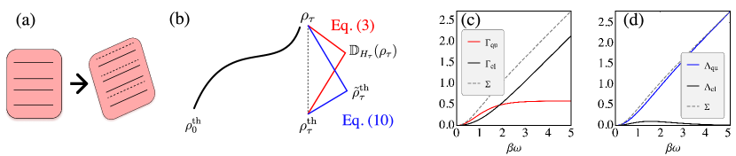
Figure 1: Difficulties in identifying the classical and quantum contributions to the entropy production. (a) A work protocol $H(g_{t})$ can modify the Hamiltonian in two ways: altering the energy level spacings, which can be viewed as a semi-classical effect, and rotating the energy eigenbasis, which is a fully quantum property with no classical counterpart. (b) The entropy production (2) compares the final state $\rho_{\tau}$ with the reference thermal state $\rho_{\tau}^{\text{th}}$. To understand its classical and quantum contributions, the splitting (3) uses an intermediate state $\mathbb{D}_{H_{\tau}}(\rho_{\tau})$. Conversely, in this paper we introduce the splitting (7), which uses the state $\tilde{\rho}_{\tau}^{\text{th}}$, in Eq. (12). (c) The contributions $\Gamma_{\text{qu}}$ and $\Gamma_{\text{cl}}$ of Eq. (3) in a minimal qubit model, as a function of $\beta\omega$, plotted using Eqs. (4) and (4) with $\theta=1.1$ (see text for details). (d) The new splitting (7) (see also Eq. (8)), which yields physically more reasonable results at low temperatures.

The entropy production $\Sigma$ in Eq. $\eqref{EntProd}$ contains contributions of both a classical and quantum nature. This is linked with the fact that the work protocol $g_{t}$ can modify the Hamiltonian $H(g)$ in two ways. On the one hand, it may alter the spacing of the energy levels; and, on the other, it may rotate the eigenvectors (Fig. 1(a)). The latter is directly associated with quantum coherence and to the fact that $[H(g_{t_{1}}),H(g_{t_{2}})]\neq 0$, for two different times $t_{1},t_{2}$. It therefore has no classical counterpart, and corresponds to a fundamental feature distinguishing classical and quantum processes. In general, these two processes will become mixed, and hence identifying how each physical process contributes to $\Sigma$ is in general a challenging task. In the literature, a popular choice is the splitting put forward in janzing2006quantum; Lostaglio2015; Santos2019; Francica2019:

$$\Sigma=\Gamma_{\text{cl}}+\Gamma_{\text{qu}},$$ (3)

where rCl Γ_cl&= S(D_H_τ(ρ_τ) —— ρ_τ^th ),
Γ_qu= S( ρ_τ —— D_H_τ(ρ_τ) ) = S(D_H_τ(ρ_τ)) - S(ρ_τ), with $\mathbb{D}_{H}(\rho)$ being the super-operator that completely dephases the state $\rho$ in the eigenbasis of $H$ (explicitly defined below, in Eq. (9)). The first term, $\Gamma_{\text{cl}}$, measures the entropic distance between the populations of the actual final state $\rho_{\tau}$ and those of the reference thermal state $\rho_{\tau}^{\text{th}}$, and is generally identified with the classical contribution. The term $\Gamma_{\text{qu}}$, in turn, is known as the relative entropy of coherence and compares the final state $\rho_{\tau}$ with the dephased state $\mathbb{D}_{H_{\tau}}(\rho_{\tau})$. It hence captures the contribution from coherences in the energy basis. By construction, $\Gamma_{\text{cl}}$ and $\Gamma_{\text{qu}}$ in Eq. (3) are both non-negative, which shows that coherences increase the entropy production in the process, as compared to a fully classical (incoherent) scenario. One should also clarify that, since the changes in populations and coherences are inevitably mixed, the terminology “classical” vs.  “quantum” is not entirely precise, nor is there a one-to-one relationship between this and the terms “populations” and “coherences”. For instance, while $\Gamma_{\text{qu}}$ depends only on the basis rotation (coherences), $\Gamma_{\text{cl}}$ depends on both the changes in energy eigenvalues, as well as the eigenbasis rotation. Notwithstanding, as we will show, in the case of infinitesimal quenches, these distinctions can be made precise.

The splitting (3), first analyzed in janzing2006quantum, has been studied in the context of the resource theory of thermodynamics Lostaglio2015, relaxation towards equilibrium Santos2019; Mohammady2020,thermodynamics of quantum optical systems Elouard2020 and work protocols in the absence of a bath Francica2019; Varizi2020; Francica2020. At the stochastic level, both $\Gamma_{\text{qu}}$ and $\Gamma_{\text{cl}}$ satisfy individual fluctuation theorems Francica2019, which is a very desirable property. Moreover, $\Gamma_{\text{cl}}$ has a resource-theoretic interpretation within the resource theory of athermality Brandao2013; Horodecki2013, while $\Gamma_{\text{qu}}$ is a natural monotone in the resource theory of coherence Baumgratz2014; Streltsov2016a. These facts make the splitting (3) a valuable tool in understanding the relative contribution of classical and quantum features to non-equilibrium processes. However, working with various models, we have observed that this splitting behaves strangely, even in some simple protocols. More specifically, we identify two main shortcomings.

The first concerns the relative magnitudes of $\Gamma_{\text{qu}}$ and $\Gamma_{\text{cl}}$: At low temperatures, $\Gamma_{\text{cl}}$ will always be much larger than $\Gamma_{\text{qu}}$. The reason is purely mathematical: $\Gamma_{\text{qu}}$ is a special kind of relative entropy because it can be expressed as a difference between two von Neumann entropies, as in the second equality of (3). As $\beta\to\infty$, $\rho_{\tau}^{\text{th}}$ tends to a pure state and hence $S(\rho_{\tau})$ tends to zero, while $S(\mathbb{D}_{H_{\tau}}(\rho_{\tau}))\in[0,\ln d]$, where $d$ is the dimension of the Hilbert space. As a consequence, $\Gamma_{\text{qu}}$ will always remain finite. The term $\Gamma_{\text{cl}}$, on the other hand, generally diverges when the support of $\rho_{\tau}$ is not contained in that of $\rho_{\tau}^{\text{th}}$ Nielsen, meaning $\Gamma_{\text{cl}}$ will grow unbounded when $\beta\to\infty$. This implies that it is impossible to construct a low-temperature process where the quantum term dominates.

More precisely, consider again the two types of drivings depicted in Fig. 1 (a): one that alters the spacing of the energy levels (associated here to a classical process), and one which may rotate eigenvectors (associated here to a quantum process). At strictly zero temperature, a Gibbs state is invariant under the first class of protocols, and hence we may expect that any entropy production in (2) has a quantum origin. However, the opposite identification arises in the splitting (3). The reason for this apparent contradiction is rather simple: The splitting (3) is not characterising whether the driving generates quantum coherence or not; rather, given a possibly coherent process, it characterises how much the final diagonal and off-diagonal terms contribute to the total entropy production.

This issue can be neatly illustrated by a minimal qubit model. Consider a qubit which starts at $H_{0}=\omega\sigma^{z}$ and is suddenly quenched ($U=1$) to $H_{\tau}=\omega(\sigma^{z}\cos\theta+\sigma^{x}\sin\theta)$ (where $\sigma^{\alpha}$ are Pauli matrices). In this quench the energy levels remain intact and all that happens is that the eigenbasis is rotated by an angle $\theta$. This is thus, by all accounts, a highly quantum process. The entropy production (2) for this model reads

$$\Sigma=2t\tanh^{-1}(t)\;\sin^{2}(\nicefrac{{\theta}}{{2}}),$$ (4)

where $t=\tanh(\beta\omega)\in[0,1]$. On the other hand, the coherent contribution $\Gamma_{\text{qu}}$ in Eq. (3), reads rCl Γ_qu&= t tanh^-1(t) - tcosθtanh^-1(tcosθ)
-12 ln(1+sinh^2(βω)sin^2θ). A plot of $\Gamma_{\text{qu}}$ and $\Gamma_{\text{cl}}=\Sigma-\Gamma_{\text{qu}}$ is shown in Fig. 1(c) as a function of $\beta\omega$, for $\theta=1.1$. As can be seen, in general both quantities are comparable in magnitude. But, as the temperature goes down ($\beta$ goes up), the classical contribution becomes increasingly larger and eventually dominates. Thus, at very low temperatures, most of $\Sigma$ comes from the population term $\Gamma_{\text{cl}}$ and very little from coherences.

The above considerations highlight the fact that splitting the total entropy production (2) in a classical and quantum contribution may be highly non-trivial, and that different splittings might provide different insights. In particular, we argue that the splitting in Eq. (3) does not appropriately distinguish coherent from non-coherent drivings (see Fig. 1), but instead characterises how populations and off-diagonal terms contribute to entropy production. In this work, we will propose a new complementary splitting that better incorporates the difference between coherent and non-coherent drivings.

A second issue with the splitting (3) concerns infinitesimal quenches. This is a very important scenario, widely studied in the context of critical systems Gambassi1106; Dorner2012; Fusco2014a; Goold2018 and quasi-isothermal processes Miller2019; Scandi2019. The idea is to analyze the entropy production perturbatively, for a small instantaneous quench of the work parameter, from $g$ to $g+\delta g$. The problem with $\Gamma_{\text{qu}}$ and $\Gamma_{\text{cl}}$ in this case is that, as will be shown, the parameter $\delta g$ appears multiplied by a factor that increases exponentially with $\beta$. Hence, the radius of convergence of $\Gamma_{\text{qu}}$ and $\Gamma_{\text{cl}}$, in $\delta g$, tends to zero exponentially fast as $\beta\to\infty$. For $\Sigma$, no such issue arises.

This is again well illustrated by the qubit example in Eqs. (4) and (4), where the quench parameter is now the angle $\theta$. We see that $\Sigma$ in (4) can be readily expanded in powers of $\theta$, for any temperature $\beta$ (or any $t=\tanh(\beta\omega)$). The same is not true for $\Gamma_{\text{qu}}$, however. The problem is in the third term of Eq. (4), which is a function of $x=\sinh^{2}(\beta\omega)\sin^{2}\theta$. This quantity appears inside a logarithm, in the form $\ln(1+x)$. However, a series expansion of $\ln(1+x)$ only converges if $|x|<1$. And since the prefactor $\sinh^{2}(\beta\omega)$ grows exponentially with $\beta$, at low temperatures, extremely small values of $\theta$ are required to validate a series expansion.

More generally, one can readily show that for $\Sigma$ this issue does not arise. If we use $\Sigma=\beta\big{(}\langle W\rangle-\Delta F\big{)}$, we find in the case of infinitesimal quenches that

$$\Sigma=\beta\text{tr}\big{\{}\Delta H\rho^{\text{th}}(g_{0})\Big{\}}-\beta\Delta F,$$ (5)

where $\Delta H=H(g_{0}+\delta g)-H(g_{0})$ and $\Delta F=F(g_{0}+\delta g)-F(g_{0})$. A series expansion of $\Sigma$ in $\delta g$ therefore amounts to two things. First, an expansion of $\Delta H$ in powers of $\delta g$, which is entirely independent of $\beta$. And second, an expansion of $F(g)$, which is an analytic and generally smooth function (except possibly at a critical point Dorner2012). Indeed, if $H(g)$ is linear in $g$, the leading order contribution to the expansion becomes Fusco2014a

$$\Sigma\simeq-\frac{1}{2}\beta\delta g^{2}\frac{\partial^{2}F}{\partial g_{0}^{2}},$$ (6)

showing that $\Sigma$ is simply proportional to the equilibrium susceptibility, a textbook quantity used throughout equilibrium statistical mechanics.

The above results show that, despite its interesting properties (individual fluctuation theorems and resource-theoretic interpretation), the splitting (3) is not a fully satisfying splitting of the entropy production into a classical and quantum contribution (in the sense described in Fig. 1 (a)). In order to capture the difference between coherent and non-coherent drivings, in this paper we propose a different splitting, which is inspired by the recent results of Scandi2019. We label it as

$$\Sigma=\Lambda_{\text{cl}}+\Lambda_{\text{qu}}.$$ (7)

The actual definitions of $\Lambda_{\text{qu}}$ and $\Lambda_{\text{cl}}$ will be given below in Sec. II and a stochastic trajectories formulation will be given in Sec. III. A comparison in the case of the minimal qubit example is also presented in Fig. 1(d). In this case, using the results of Sec. II, one finds the following elegant expression for $\Lambda_{\text{qu}}$ (to be contrasted with Eq. (4)):

$$\Lambda_{\text{qu}}=\frac{1}{2}\ln\left(\frac{1-\tanh^{2}(\beta\omega\cos\theta)}{1-\tanh^{2}(\beta\omega)}\right).$$ (8)

As seen in Fig. 1(d), $\Lambda_{\text{qu}}$ and $\Lambda_{\text{cl}}$ behave as desired: Since the process is highly coherent, $\Lambda_{\text{cl}}$ is very small; and as the temperature goes down, $\Lambda_{\text{qu}}$ grows monotonically, showing that cold processes have higher contributions from the coherences.

The features discussed in Fig. 1 are not restricted to quenches. To illustrate that we show in Fig. 2 another qubit example, where the process is assumed to be cyclic, with $H_{\tau}=H_{0}=\omega\sigma_{z}$, and the unitary is taken to be generated by an $x$-pulse with a duration $\tau$; that is, $U=e^{-i\tau(H_{0}+h_{x}\sigma_{x})}$, where $h_{x}$ is the pulse intensity. Fig. 2 illustrates the results for $\omega=1$, $h_{x}=1.3$ and two choices of $\tau$: in the upper panels $\tau=0.4$ and in the lower panels $\tau=1$. The results show that for (3) the behavior is always roughly the same, with $\Gamma_{\text{cl}}$ always eventually dominating at low temperatures. Conversely, for the new splitting (7) a richer competition is observed. Depending on the parameters we may either have $\Lambda_{\text{qu}}$ dominating, or $\Lambda_{\text{cl}}$, or both.

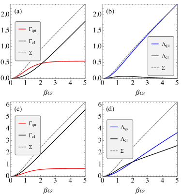
Figure 2: Splitting of the entropy production in a cyclic qubit model, $H_{\tau}=H_{0}=\omega\sigma_{z}$. The unitary is generated by an $x$-pulse with a duration $\tau$; that is, $U=e^{-i\tau(H_{0}+h_{x}\sigma_{x})}$, where $h_{x}$ is the pulse intensity. The curves were computed using Eqs. (11), (11), (11), (12) and (12), with $\omega=1$, $h_{x}=1.3$ and two different values of $\tau$: in (a),(b) $\tau=0.4$ and in (c),(d) $\tau=1$.

As we will show in this paper, our new splitting (7) more accurately distinguishes which part of the entropy production is generated by a commuting or non-commuting drive. This provides a complementary approach to the standard splitting in Eq. (3), which instead describes how populations and coherences in the final state contribute to entropy production. On the other hand, we also note that $\Lambda_{\text{qu}}$ and $\Lambda_{\text{cl}}$ do not share some of the nice properties of $\Gamma_{\text{qu}}$ and $\Gamma_{\text{cl}}$. First, $\Lambda_{\text{qu}}$ cannot be directly linked with a monotone for coherence or asymmetry Streltsov2016a. Second, while $\Lambda_{\text{cl}}$ always satisfies an individual fluctuation theorem, $\Lambda_{\text{qu}}$ only does so in the case of infinitesimal quenches. Different properties of each splitting are highlighted in Table 1. We also show that for infinitesimal quenches at high temperatures, both splittings coincide - see Sec. LABEL:ssec:stoch_infinitesimal.

To illustrate the usefulness of our results, we analyze our new splitting in two quantum many-body problems. Previous works have focused on the behaviour of the statistics of work and entropy production $\Sigma$ for quantum quenches Gambassi1106; Dorner2012; Fusco2014a; PhysRevE92022108; Goold2018; PhysRevA99043603, with emphasis in quantum phase transitions Dorner2012; Mascarenhas1307; PhysRevA95063615; Pagnelli; PhysRevE98022107; PhysRevB93201106; Bayocboc2015; PhysRevE97052148; Nigro. Motivated by this, we analyze in Sec. LABEL:sec:XYmodel the transverse field Ising model (TFIM), and discuss the behavior of (7) in the vicinity of the quantum critical point. This is complementary to the analysis put forth in Varizi2020, which studied Eq. (3). Then, in Sec. LABEL:sec:LMG, we consider a macrospin of varying size and focus on the full statistics of $\Lambda_{\text{qu}}$ and $\Lambda_{\text{cl}}$, including their probability distributions and their first four cumulants. We finish with conclusions and future perspectives in Sec. LABEL:sec:conclusion.

Table 1: Comparison between $\Lambda_{\text{qu}}$, $\Lambda_{\text{cl}}$, $\Gamma_{\text{qu}}$ and $\Gamma_{\text{cl}}$.

	$\Lambda_{\text{qu}}$	$\Lambda_{\text{cl}}$	$\Gamma_{\text{qu}}$	$\Gamma_{\text{cl}}$
Fluctuation Theorem	✗	✓	✓	✓
Fluctuation Theorem when $\Delta H\to 0$	✓		✓
Analytic when $\Delta H\to 0$ and low $T$	✓		✗
Resource-theoretic interpretation	✗		✓
Vanishing for commuting protocols	✓	-	✓	-
Dominant for highly coherent protocols	✓	-	✗	-
Dominant at low temperatures	✓	-	✗	-

II Splittings of the entropy production

In this section we introduce our alternative splitting of the entropy production [Eq. (7)]. We focus for now at the level of averages; the corresponding stochastic formulation will be presented in Sec. III.

Let $\mathcal{O}$ denote any Hermitian observable and decompose it as $\mathcal{O}=\sum_{\alpha}o_{\alpha}\Pi_{\alpha}$, where $\Pi_{\alpha}$ are projectors onto the subspaces with eigenvalues $o_{\alpha}$. We define the dephasing operation

$$\mathbb{D}_{\mathcal{O}}(\bullet)=\sum\limits_{\alpha}\Pi_{\alpha}\bullet\Pi_{\alpha}.$$ (9)

The rationale of the splitting Eq. (3) was to introduce an intermediate step, associated with the state $\mathbb{D}_{H_{\tau}}(\rho_{\tau})$ (Fig. 1(b)). This represents the final state $\rho_{\tau}$ dephased in the eigenbasis of the final Hamiltonian. If the process generates coherences, this state will differ from the actual final state $\rho_{\tau}$ and their entropic distance will be precisely $\Gamma_{\text{qu}}$ in Eq. (3).

For convenience, we introduce the non-equilibrium free energy, associated with the final Hamiltonian $H_{\tau}$

$$F(\rho)=\text{tr}\Big{\{}H_{\tau}\rho\Big{\}}-TS(\rho).$$ (10)

Non-equilibrium free energies depend on two parameters, $H$ and $\rho$. However, in this paper, we will henceforth only need free energies defined with respect to $H_{\tau}$, so we write it more simply as $F(\rho)$. In terms of $F$, the entropy production (2) can be written as

$$\Sigma=\beta\Big{\{}F(\rho_{\tau})-F(\rho_{\tau}^{\text{th}})\Big{\}},$$ (11)

Similarly, one can also express $\Gamma_{\text{qu}}$ and $\Gamma_{\text{cl}}$ in terms of free energy differences. Since $\text{tr}\big{\{}H_{\tau}\mathbb{D}_{H_{\tau}}(\rho_{\tau})\big{\}}=\text{tr}\big{\{}H_{\tau}\rho_{\tau}\big{\}}$, one finds that rCl Γ_qu&= β{ F(ρ_τ) - F(D_H_τ(ρ_τ))},
Γ_cl= β{ F(D_H_τ(ρ_τ)) - F (ρ_τ^th) }, which clearly add up to $\Sigma$.

The splitting (3) uses $\mathbb{D}_{H_{\tau}}(\rho_{\tau})$ as intermediate state. Our new splitting (7) follows a similar logic, but in reverse: Instead of working with $\rho_{\tau}$ dephased in the basis of $H_{\tau}$, we work with $H_{\tau}$ dephased in the basis of $\rho_{\tau}$. More precisely, we define

$$\tilde{\rho}_{\tau}^{\text{th}}=\frac{\exp\{-\beta~{}\mathbb{D}_{\rho_{\tau}}(H_{\tau})\}}{\text{tr}\Big{(}\exp\{-\beta~{}\mathbb{D}_{\rho_{\tau}}(H_{\tau})\}\Big{)}},$$ (12)

which is a thermal state based only on the incoherent part of $H_{\tau}$, in the basis of $\rho_{\tau}$ (as a consequence, $[\tilde{\rho}_{\tau}^{\text{th}},\rho_{\tau}]=0$). With this in mind, we now define rCl Λ_cl&= β{ F(ρ_τ) - F(~ρ_τ^th)},
Λ_qu= β{F(~ρ_τ^th) - F(ρ_τ^th)}, which add up to $\Sigma$, as in Eq. (7). The first term, $\Lambda_{\text{cl}}$, compares the two commuting states $\rho_{\tau}$ and $\tilde{\rho}_{\tau}^{\text{th}}$ and is hence associated with their population mismatch. The nonnegativity of $\Lambda_{\text{cl}}$ becomes evident by noting that it can also be written as

$$\Lambda_{\text{cl}}=S(\rho_{\tau}||\tilde{\rho}_{\tau}^{\text{th}}).$$ (13)

The term $\Lambda_{\text{qu}}$, on the other hand, compares $\rho_{\tau}^{\text{th}}\propto e^{-\beta H_{\tau}}$ with $\tilde{\rho}_{\tau}^{\text{th}}\propto e^{-\beta\mathbb{D}_{\rho_{\tau}}(H_{\tau})}$. Unlike $\Lambda_{\text{cl}}$, the contribution $\Lambda_{\text{qu}}$ cannot be written as a relative entropy. In fact, written down explicitly, it reads

$$\Lambda_{\text{qu}}=\text{tr}\Big{\{}\rho_{\tau}\Big{(}\ln\tilde{\rho}_{\tau}^{\text{th}}-\ln\rho_{\tau}^{\text{th}}\Big{)}\Big{\}}.$$ (14)

Notwithstanding, as shown in Appendix LABEL:appsec:nonnegA, it turns out that $\Lambda_{\text{qu}}$ is still non-negative, and zero if and only if $[H_{\tau},\rho_{\tau}]=0$.

Throughout this paper we will provide several additional justifications as to why the choices (12) and (12) are physically reasonable, starting in Sec. II.1. But before doing so, let us briefly revisit the minimal qubit model defined above Eq. (4). The process is a quench ($U=1$), so $\rho_{\tau}=\rho_{0}^{\text{th}}$. Hence, all we need to do in order to compute $\Lambda_{\text{qu}}$ is to dephase the final Hamiltonian $H_{\tau}=\omega(\sigma^{z}\cos\theta+\sigma^{x}\sin\theta)$ in the basis of $\rho_{0}^{\text{th}}$. Or, what is equivalent, in the basis of $H_{0}$. The result is thus simply $\mathbb{D}_{\rho_{\tau}}(H_{\tau})=\omega\cos(\theta)\sigma_{z}$. Using this in (12) yields Eq. (8), which is the result plotted in Fig. 1(d) and discussed in Sec. I.

II.1 Infinitesimal quenches

The physics of the problem becomes particularly simpler in the case of infinitesimal quenches. We therefore now specialize the above results to this scenario. This will provide strong justifications in favor of the new splitting (7). Furthermore, in this limit the splitting (7) becomes equivalent to the one recently put forward in Scandi2019. More precisely, in Scandi2019 the authors describe quasi-isothermal processes as a series of infinitesimal quenches, and in particular consider how $\Sigma$ splits into a classical and quantum contribution. Focusing on a single infinitesimal quench, both approaches become directly comparable and, as we will show, agree with each other.

We thus analyze what happens if we take $U=1$, and assume that $H$ changes only by a small amount $\Delta H$ (i.e., we write $H_{\tau}=H_{0}+\Delta H$). Since $U=1$, the state of the system remains unchanged: $\rho_{\tau}=\rho^{\text{th}}_{0}$. Therefore, dephasing $H_{\tau}$ in the basis of $\rho_{\tau}$ is equivalent to dephasing in the basis of $H_{0}$:

$$\mathbb{D}_{\rho_{\tau}}(H_{\tau})=\mathbb{D}_{\rho^{\text{th}}_{0}}(H_{\tau})=\mathbb{D}_{H_{0}}(H_{\tau}).$$ (15)

Let us define the dephased (incoherent) and coherent parts of the perturbation $\Delta H$, in the initial energy basis, $\Delta H^{\text{d}}=\mathbb{D}_{H_{0}}(\Delta H)$ and $\Delta H^{\text{c}}=H_{\tau}-\mathbb{D}_{H_{0}}(H_{\tau})$. Then, following a procedure detailed in Appendix B of Ref. Scandi2019, one may show that, rCl ~ρ^th _τ &= ρ^th_0 - β  J_ρ^th_0 [ΔH^d - ⟨ΔH^d⟩_0] + O(ΔH^2),
ρ^th_τ = ρ^th_0 - β  J_ρ^th_0 [ΔH - ⟨ΔH⟩_0] + O(ΔH^2), where $\langle\ldots\rangle_{0}=\text{tr}\{\ldots\rho_{0}^{\text{th}}\}$ and $\mathbb{J}_{\rho}$ is a super-operator defined as

$$\mathbb{J}_{\rho}[\bullet]=\int_{0}^{1}\rho^{t}\bullet\rho^{1-t}\mathrm{d}t.$$ (16)

We see that both $\rho_{\tau}^{\text{th}}$ and $\tilde{\rho}_{\tau}^{\text{th}}$ can be expanded essentially in a power series in $\beta\Delta H$. Conversely, the same is not true for the state $\mathbb{D}_{H_{\tau}}(\rho_{0}^{\text{th}})$ entering (11) and (11). In fact, one may show that to order $\Delta H$

$$\mathbb{D}_{H_{0}+\Delta H}(\rho_{0}^{\text{th}})=\rho_{0}^{\text{th}}+\lim_{s\to\infty}\frac{i}{s}\int_{0}^{s}\mathrm{d}t\int_{0}^{1}\mathrm{d}x\,t~{}e^{-ixH_{0}t}[\rho_{0}^{\text{th}},\Delta H]e^{ixH_{0}t}.$$ (17)

Even though this is an expansion in $\Delta H$, the dependence on $\beta$ enters in a highly non-trivial way. This explains the non-analytic behavior of $\Gamma_{\text{cl}}$ and $\Gamma_{\text{qu}}$ at low temperatures, discussed in Sec. I.

Plugging (II.1)-(II.1) in Eqs. (2), (13) and (14) leads, up to second order, to rCl Σ&= β22 tr ΔH   J_ρ^th_0 [ΔH - ⟨ΔH⟩_0] = Λ_cl+ Λ_qu,
Λ_cl= β22 tr ΔH^d   J_ρ^th_0 [ΔH^d - ⟨ΔH^d⟩_0] ,
Λ_qu= β22 tr ΔH^c   J_ρ^th_0 [ΔH^c] , where we used the fact that $\langle\Delta H^{\text{d}}\rangle_{0}=\langle\Delta H\rangle_{0}$. The interesting aspect of these results is that, within this infinitesimal quench limit, $\Lambda_{\text{cl}}$ and $\Lambda_{\text{qu}}$ are found to be related to $\Sigma$ via the simple separation of the perturbation, $\Delta H=\Delta H^{\text{d}}+\Delta H^{\text{c}}$, into a dephased and a coherent part. These results also coincide with the splitting proposed in Scandi2019.

An additional justification for the splitting (7) can be given in terms of the fluctuation-dissipation relation (FDR). As shown in Refs. Miller2019; Scandi2019, Eq. (II.1) can also be written as

$$\Sigma=\frac{1}{2}\beta^{2}\,\text{Var}_{0}[\Delta H]-\beta\mathcal{Q},$$ (18)

where $\text{Var}_{0}[\Delta H]=\langle\Delta H^{2}\rangle_{0}-\langle\Delta H\rangle_{0}^{2}$, is the variance of the perturbation, and

$$\mathcal{Q}=\frac{\beta}{2}\int_{0}^{1}\mathrm{d}y\,I^{y}(\rho^{\text{th}}_{0},\Delta H)\geqslant 0,$$ (19)

is a measure of quantum coherence, associated with the so-called Wigner-Yanase-Dyson skew information Petz2002

$$I^{y}(\varrho,X)=-\frac{1}{2}\text{tr}{[\varrho^{y},X][\varrho^{1-y},X]}.$$ (20)

For incoherent processes one recovers the usual FDR $\Sigma=\frac{\beta^{2}}{2}\text{Var}_{0}[\Delta H]$ Jarzynski1997. But when the process is coherent, the FDR is broken by a term $-\beta\mathcal{Q}$. Repeating the same procedure for $\Lambda_{\text{cl}}$ and $\Lambda_{\text{qu}}$, one readily finds that

$$\Lambda_{\text{cl}}=\frac{\beta^{2}}{2}\,\text{Var}_{0}[\Delta H^{\text{d}}],\qquad\Lambda_{\text{qu}}=\frac{\beta^{2}}{2}\,\text{Var}_{0}[\Delta H^{\text{c}}]-\beta\mathcal{Q}.$$ (21)

Whence, $\Lambda_{\text{cl}}$ always satisfies a standard FDR, and all violations are associated to $\Lambda_{\text{qu}}$. This provides additional justification as to why $\Lambda_{\text{qu}}$ is referred to as a quantum contribution.

In the case of high temperatures ($\beta\to 0$), one may show that $\mathcal{Q}\sim\mathcal{O}(\beta)^{3}$. Moreover, the state entering the variances in Eq. (21) can be replaced with the maximally mixed state $\mathbb{I}/d$. As a consequence, we find that to leading order in $\beta$,

$$\Lambda_{\text{cl}}=\frac{\beta^{2}}{2}\,\text{Var}_{\mathbb{I}/d}[\Delta H^{\text{d}}],\qquad\Lambda_{\text{qu}}=\frac{\beta^{2}}{2}\,\text{Var}_{\mathbb{I}/d}[\Delta H^{\text{c}}].$$ (22)

Both contributions are thus found to scale as $\beta^{2}$ in this limit, which agrees with the observations in Fig. 1(c) and (d). However, their relative contribution will be determined by the variance of $\Delta H^{d}$ and $\Delta H^{c}$ in the maximally mixed state; hence, which term will be dominant will depend on the details of the process (either a commuting or a non-commuting drive). This is also expected to remain true for general drives.

III Stochastic trajectories

We now discuss how to formulate the splittings (3) and (7) at the level of stochastic trajectories, based on a standard two-point measurement (TPM) scheme Talkner2007. Since $\Sigma=\beta(\langle W\rangle-\Delta F)$, the statistics of $\Sigma$ can be obtained solely from measurements in the eigenbasis of the initial and final Hamiltonians. As first shown in Francica2019, a major advantage of the original splitting (3) is that this remains true when assessing the individual contributions $\Gamma_{\text{cl}}$ and $\Gamma_{\text{qu}}$; that is, no additional measurements are necessary. As we will now show, the same is also true for $\Lambda_{\text{cl}}$ and $\Lambda_{\text{qu}}$ [Eq. (7)]. This means that both splittings can be assessed, at the stochastic level, with the same amount of information as a standard TPM.

Irrespective of the splitting one is interested in, the protocol may therefore be described as follows. Initially the system is in the thermal state $\rho_{0}^{\text{th}}$, associated with the Hamiltonian $H_{0}=\sum_{i}\epsilon_{i}^{0}|i_{0}\rangle\langle i_{0}|$. The first measurement is performed in the basis $|i_{0}\rangle$, which occurs with probability $p_{i}^{0}=e^{-\beta\epsilon_{i}^{0}}/Z_{0}$. Conversely, the second measurement is performed at time $\tau$, after the map (1), and in the eigenbasis of the final Hamiltonian $H_{\tau}=\sum_{j}\epsilon_{j}^{\tau}|j_{\tau}\rangle\langle j_{\tau}|$. The bases $\{|i_{0}\rangle\}$ and $\{|j_{\tau}\rangle\}$ are, in general, not compatible.

The conditional probability of finding the system in $|j_{\tau}\rangle$ given that it was initially in $|i_{0}\rangle$ is $|\langle j_{\tau}|U|i_{0}\rangle|^{2}$. The probability associated with the forward protocol $|i_{0}\rangle\to|j_{\tau}\rangle$ is thus $\mathcal{P}_{F}[i,j]=|\langle j_{\tau}|U|i_{0}\rangle|^{2}~{}p_{i}^{0}$. The dynamics is defined as being incoherent when $|\langle j_{\tau}|U|i_{0}\rangle|^{2}=\delta_{i,j}$, which means $U$ is not able to generate transitions between states of the initial and final Hamiltonians. Similarly, in the backward protocol the system starts in $\rho_{\tau}^{\text{th}}$ and one measures first in the basis of $H_{\tau}$, yielding $|j_{\tau}\rangle$ with probability $p_{j}^{\tau}=e^{-\beta\epsilon_{j}^{\tau}}/Z_{\tau}$. The time-reversed unitary $U^{\dagger}$ is then applied, after which one measures in the basis $|i_{0}\rangle$ of $H_{0}$. This yields the backward distribution $\mathcal{P}_{B}[i,j]=|\langle i_{0}|U^{\dagger}|j_{\tau}\rangle|^{2}p_{j}^{\tau}$.

The entropy production associated to the trajectory $|i_{0}\rangle\to|j_{\tau}\rangle$ is now defined as usual:

$$\sigma[i,j]=\ln\frac{\mathcal{P}_{F}[i,j]}{\mathcal{P}_{B}[i,j]}=\ln p_{i}^{0}/p_{j}^{\tau}.$$ (23)

The second equality follows from the fact that $|\langle i_{0}|U^{\dagger}|j_{\tau}\rangle|^{2}=|\langle j_{\tau}|U|i_{0}\rangle|^{2}$. As a consequence, $\sigma[i,j]$ depends only on the equilibrium populations $p_{i}^{0}$ and $p_{j}^{\tau}$, associated with the initial and final Hamiltonians. As can be readily verified, $\langle\sigma[i,j]\rangle=\sum_{i,j}\sigma[i,j]\mathcal{P}_{F}[i,j]=\Sigma$, returns precisely Eq. (2). In addition, $\sigma[i,j]$ also satisfies an integral fluctuation theorem $\langle e^{-\sigma}\rangle=1$ (see Eq. (LABEL:CGF_sigma) for more details).

III.1 Stochastic definitions for the splittings (3) and (7)

Following Francica2019, we now define stochastic quantities associated to $\Gamma_{\text{cl}}$ and $\Gamma_{\text{qu}}$. In order to do that, we first write the dephased state $\mathbb{D}_{H_{\tau}}(\rho_{\tau})$ as $\mathbb{D}_{H_{\tau}}(\rho_{\tau})=\sum_{j}q_{j}^{\tau}|j_{\tau}\rangle\langle j_{\tau}|$, where

$$q_{j}^{\tau}=\langle j_{\tau}|\rho_{\tau}|j_{\tau}\rangle=\sum\limits_{i}|\langle j_{\tau}|U|i_{0}\rangle|^{2}p_{i}^{0}.$$ (24)

In passing, we note that $q_{j}^{\tau}=\sum_{i}\mathcal{P}_{F}[i,j]$, so $q_{j}^{\tau}$ can also be interpreted as the marginal distribution of the final measurement. As shown in Francica2019, we may now define rCl γ_cl[i,j] &= lnq_j^τ/p_j^τ,
γ_qu[i,j] = lnp_i^0/q_j^τ. Clearly $\gamma_{\text{cl}}[i,j]+\gamma_{\text{qu}}[i,j]=\sigma[i,j]$, which is the stochastic analog of (3). Moreover, $\langle\gamma_{\text{cl}}[i,j]\rangle=\Gamma_{\text{cl}}$ and $\langle\gamma_{\text{qu}}[i,j]\rangle=\Gamma_{\text{qu}}$.

Similarly, we construct stochastic quantities for the new quantities $\Lambda_{\text{cl}}$ and $\Lambda_{\text{qu}}$ in Eq. (7). The central object now is the thermal state $\tilde{\rho}_{\tau}^{\text{th}}$, defined in Eq. (12) and associated with the Hamiltonian $\mathbb{D}_{\rho_{\tau}}(H_{\tau})$. Since the system evolves unitarily, $\rho_{\tau}=U\rho_{0}^{\text{th}}U^{\dagger}=\sum_{i}p_{i}^{0}|\psi_{i}\rangle\langle\psi_{i}|$, where $|\psi_{i}\rangle=U|i\rangle$. That is, $\rho_{\tau}$ has the same populations $p_{i}^{0}$ as $\rho_{0}^{\text{th}}$, but a rotated eigenbasis. Based on this, we can now write Eq. (12) as

$$\tilde{\rho}_{\tau}^{\text{th}}=\sum_{i}\tilde{p}_{i}^{\tau}|\psi_{i}\rangle\langle\psi_{i}|,\qquad\tilde{p}_{i}^{\tau}=e^{-\beta(\tilde{\epsilon}_{i}^{\tau}-F(\tilde{\rho}_{\tau}^{\text{th}}))},$$ (25)

where $\tilde{\epsilon}_{i}^{\tau}=\langle\psi_{i}|H_{\tau}|\psi_{i}\rangle$ are the eigenvalues of the dephased Hamiltonian $\mathbb{D}_{\rho_{\tau}}(H_{\tau})$ and $F(\tilde{\rho}_{\tau}^{\text{th}})$ is the same free energy as that appearing in Eq. (12). We then define rCl λ_cl[i,j] = lnp