Tagged active particle: probability distribution in a slowly varying external potential is determined by effective temperature obtained from the Einstein relation

Abstract

We derive a distribution function for the position of a tagged active particle in a slowly varying in space external potential, in a system of interacting active particles. The tagged particle distribution has the form of the Boltzmann distribution but with an effective temperature that replaces the temperature of the heat bath. We show that the effective temperature that enters the tagged particle distribution is the same as the effective temperature defined through the Einstein relation, i.e. it is equal to the ratio of the self-diffusion and tagged particle mobility coefficients. This shows that this effective temperature, which is defined through a fluctuation-dissipation ratio, is relevant beyond the linear response regime. We verify our theoretical findings through computer simulations. Our theory fails when an additional large length scale appears in our active system. This length scale is associated with long-wavelength density fluctuations that emerge upon approaching motility-induced phase separation.

I Introduction

Equilibrium statistical mechanics provides us with explicit expressions for many-particle probability distributions for systems that are either isolated or in contact with one or more reservoirs Chandler . Probably the most often invoked distribution is the Boltzmann distribution $\propto\exp\left(-\mathcal{H}/T\right)$ describing an equilibrium system with Hamiltonian $\mathcal{H}$ at temperature $T$ (here and in the following we use units such that Boltzmann constant is equal to 1, $k_{B}=1$). A lot of effort, analytical and/or numerical, is required to obtain from this distribution explicit results for measurable properties of a system of interacting particles, but at least we are provided with an explicit starting point for such an effort.

In contrast, for out-of-equilibrium stationary states we do not have such a starting point. If we were to follow the same route as in equilibrium statistical mechanics, we would need to derive an exact or approximate expression for a non-equilibrium steady-state many-particle distribution and then use it to calculate measurable properties of the non-equilibrium system considered. It is rather unlikely that a general formula for such a distribution exists. Conversely, it is very likely that if it were to be found it would be more complicated than the many-particle equilibrium distribution.

On the other hand, it is not clear that we need the full many-particle distribution. Most of the interesting properties of many-particle systems can be expressed in terms of reduced distribution functions, i.e. pair distribution $g(r)$ and its generalizations to groups of more than two particles. To calculate these properties one can attempt to derive approximate formulas for the reduced distribution for specific non-equilibrium steady states. We note that in some cases the reduced distributions in non-equilibrium steady states can be measured directly. For example, in the iconic scattering experiment of Clark and Ackerson ClarkAckerson the static structure factor, i.e. the Fourier transform of the pair distribution function, of a sheared colloidal suspension was measured. This experiment inspired a number of other experimental, computational, and theoretical studies of the pair structure in colloidal systems under shear.

In the present paper we focus on a class of non-equilibrium systems that have attracted a lot of attention in last decade, active matter systems  Ramaswamy2010 ; Vicsek2012 ; Marchetti2013 ; Elgeti2015 ; Bechinger2016 ; Needleman2017 ; Ramaswamy2017 . The constituents of these systems consume energy and as a result move in a systematic way. Examples include assemblies of bacteria or of cells, suspensions of Janus colloidal particles, swarms of insects and flocks of birds. These constituents are often modeled as active or self-propelled particles, which move in a systematic way on short-time scales and in a diffusive way on long-time scales. Importantly, their dynamics breaks detailed balance, and thus their stationary states are profoundly different from equilibrium states. Needless to say, many-particle probability distributions describing these stationary states are not known explicitly. Several different approximate expressions for such distributions have been proposed and tested Maggi2015 ; Farage2015 ; Rein2016 . In spite of a considerable body of work it is not yet clear which approximate method is most promising.

In some limits the problem of finding the many-particle stationary distribution for systems of interacting active particles may simplify. For example, in a recent remarkable contribution de Pirey et al. dePirey2019 showed that in the large dimensional limit, higher-than-two-particle correlations are negligible and used this finding to derive an exact expression for the pair distribution function.

Here we are interested in a more restricted problem. We consider a system of interacting active particles in the presence of an external potential that varies slowly in space and acts on one particle only, the tagged particle. The question we want to answer is, what is the spatial distribution of tagged particle’s position? For an equilibrium system at constant temperature this problem has a simple answer; the tagged particle distribution is the Boltzmann distribution for a single particle in an external potential at the temperature of the system. Remarkably, this answer is valid irrespectively of the spatial dependence of the external potential.

We show that for a system of interacting active particles in the limit of slowly varying in space external potential the tagged particle distribution also has a form of the Boltzmann distribution. However, in this case the role of the temperature is played by a variable that is a ratio of two quantities for which we derive exact albeit formal expressions. Importantly, we show that these quantities are two well-known parameters describing tagged particle dynamics, the self-diffusion coefficient and the tagged particle mobility. Thus, the role of the temperature in our tagged particle distribution is played by the ratio of the self-diffusion and mobility coefficients, which has long been recognized as one of the so-called effective temperatures Cugliandolo2011 , the Einstein relation temperature.

Recall that in equilibrium statistical mechanics the temperature appears not only in equilibrium probability distributions but also in other relations. In particular, it appears as a proportionality constant in fluctuation-dissipation relations, which connect fluctuations in equilibrium and linear response functions due to weak external perturbations Chandler ; Kubo1966 ; MarconiPuglisi2008 . The derivation of these relations relies upon the equilibrium form of the many-particle distribution and in out-of-equilibrium systems these relations are generally not valid. In the nineties Cugliandolo, Kurchan and Peliti Cugliandolo1997 realized that the violation of fluctuation-dissipation relations can be used to define temperature-like quantities, which they called effective temperatures. These temperatures are defined through the fluctuation-dissipation ratios, i.e. the ratios of the properties characterizing fluctuations and linear response/dissipation in non-equilibrium states. Importantly, Cugliandolo, Kurchan and Peliti showed that in a slowly relaxing model system, the effective temperature determines the direction of the heat flow. Following this work, a number of different effective temperatures and their properties have been investigated in globally driven non-equilibrium stationary states Berthier2002 ; Crisanti2003 and non-stationary aging systems Barrat1999 ; Leuzzi2009 . Remarkably, in driven glassy systems it was found that several seemingly different temperatures have the same value Berthier2002 , which hinted that there might be a unique effective temperature, at least in this case.

More recently, the Einstein effective temperature, which is defined as the ratio of the self-diffusion and tagged particle mobility coefficients, has been used to characterize some properties of active matter systems Levis2015 ; Szamel2017 ; Petrelli2020 ; Loi2008 . In particular, some of us argued that the difference between the Einstein temperature and the so-called active temperature, which characterizes the strength of the self-propulsions, is a good measure of the departure of an active system from equilibrium FlennerSzamel2020 .

Since effective temperatures are defined through the ratio of fluctuations in a steady state to a function describing linear response of this state to a weak external perturbation, it is not clear whether these temperatures can also describe any non-linear response of steady states. Two studies showed the usefulness of the Einstein effective temperature for non-linear response. First, Hayashi and Sasa Hayashi2004 showed that the Einstein temperature determines the large scale distribution of a single Brownian particle moving in a tilted periodic potential. Second, Szamel and Zhang SzamelZhang2011 showed that the Einstein temperature determines the tagged particle density distribution in a slowly varying in space external potential in a system of interacting Brownian particles under steady shear. In both cases the important assumption was the slow variation in space of the external potential, but there was no restriction on its strength.

The present result is similar to that of Ref. SzamelZhang2011 in that we assume that the external potential acting on the tagged particle is slowly varying in space and we show that the density distribution is determined by the Einstein temperature. The important difference with this earlier work is in that the present system is athermal, locally driven by self-propulsions of individual particles, and isotropic.

We verify our theoretical results by performing computer simulations of an active system with an external potential. We show that the the theory is valid as long as the spatial scale on which the tagged particle density distribution varies is the longest relevant length scale in the problem. When the density correlation length becomes large, due to the incipient motility-induced phase separation, the assumption behind our theory becomes invalid and numerical results show that the theory fails.

The paper is organized as follows. In Sec. II we present our theoretical derivation. In Sec. III, we describe our computer simulation model and describe our numerical procedures in Sec. III.1, and then we present the results and discuss the limitations of our theory in Sec. III.2. Finally, we conclude the paper with an overview of our results in Sec. IV.

II Theoretical Derivation

To derive the equation describing the tagged active particle density distribution in a slowly varying in space external potential we use a gradient expansion. Specifically, we use a version of the celebrated Chapman-Enskog expansion that was originally introduced to derive hydrodynamic equations and the expressions for transport coefficients from the Boltzmann kinetic equation Resibois . The specific implementation of the Chapman-Enskog procedure that we use is inspired by Titulaer’s Titulaer1978 derivation of the generalized Smoluchowski equation, which describes diffusive motion of a colloidal particle in an external potential, from the Fokker-Planck equation, which describes the motion of the same particle on a shorter time scale, using both particle’s positions and momentum. Our present derivation is similar to that used earlier SzamelZhang2011 to obtain an equation describing the tagged particle distribution in a sheared colloidal suspension.

To make the derivation concrete we need to specify the active particles model. We consider a system of active Ornstein-Uhlenbeck particles (AOUPs) Szamel2014 ; Maggi2015 ; Fodor2016 . These particles move in a viscous medium, without inertia, under the combined influence of the inter-particle forces and self-propulsions, with the latter evolving according to the Ornstein-Uhlenbeck stochastic process. The equations of motions read

$$\dot{\mathbf{r}}_{i} = \mu_{0}\left[\mathbf{F}_{i}+\mathbf{f}_{i}\right],$$ (1)

$$\tau_{p}\dot{\mathbf{f}}_{i} = \mathbf{f}_{i}+\boldsymbol{\eta}_{i}.$$ (2)

In Eq. (1) $\mathbf{r}_{i}$ is the position of particle $i$, $\mu_{0}$ is the mobility coefficient of an isolated particle, which is the inverse of the isolated particle’s friction coefficient, $\mu_{0}=\xi_{0}^{-1}$, $\mathbf{F}_{i}$ is the force acting on particle $i$ due to all other particles,

$$\mathbf{F}_{i}=\sum_{j\neq i}\mathbf{F}(\mathbf{r}_{ij}),$$ (3)

where $\mathbf{r}_{ij}=\mathbf{r}_{i}-\mathbf{r}_{j}$ and $\mathbf{F}(\mathbf{r})=-\partial_{\mathbf{r}}V(r)$ with $V(r)$ being the two-body potential, and $\mathbf{f}_{i}$ is the self-propulsion. In Eq. (2) $\tau_{p}$ is the persistence time of the self-propulsion and $\boldsymbol{\eta}_{i}$ is the internal Gaussian noise with zero mean and variance $\left<\boldsymbol{\eta}_{i}(t)\boldsymbol{\eta}_{j}(t^{\prime})\right>_{\mathrm{noise}}=2\xi_{0}k_{B}T_{a}\mathbf{I}\delta_{ij}\delta(t-t^{\prime})$, where $\left<\ldots\right>_{\mathrm{noise}}$ denotes averaging over the noise distribution, $T_{a}$ is the “active” temperature, and $\mathbf{I}$ is the unit tensor. The active temperature characterizes the strength of the self-propulsion. In addition, it determines the long-time diffusion coefficient of an isolated AOUP, $D_{0}=T_{a}\mu_{0}\equiv T_{a}/\xi_{0}$.

We assume that there is a slowly varying in space external potential, $\Phi(\mathbf{r}_{1})$, acting on particle 1. This particle will be referred to as the tagged particle. The external potential results in an additional term, $-\partial_{\mathbf{r}_{1}}\Phi(\mathbf{r}_{1})$, in the equation of motion for the tagged particle,

$$\dot{\mathbf{r}}_{1} = \mu_{0}\left[\mathbf{F}_{1}-\partial_{\mathbf{r}_{1}}\Phi(\mathbf{r}_{1})+\mathbf{f}_{1}\right],$$ (4)

$$\tau_{p}\dot{\mathbf{f}}_{1} = \mathbf{f}_{1}+\boldsymbol{\eta}_{1}.$$ (5)

We assume that the systems described by equations of motion (1-4) can reach a stationary state. The $N$-particle stationary state distribution of positions and self-propulsions, $P_{\mathrm{s}}^{\Phi}$, satisfies the following equation,

$$\left[\Omega_{s}+\partial_{\mathbf{r}_{1}}\cdot\mu_{0}\left(\partial_{\mathbf{r}_{1}}\Phi(\mathbf{r}_{1})\right)\right]P_{\mathrm{s}}^{\Phi}\left(\mathbf{r}_{1},\mathbf{f}_{1},\ldots,\mathbf{r}_{N},\mathbf{f}_{N}\right)=0.$$ (6)

Here $\Omega_{s}$ is the evolution operator that corresponds to the unperturbed equations of motion,

$$\Omega_{\mathrm{s}}\left(\mathbf{r}_{1},\mathbf{f}_{1},\ldots,\mathbf{r}_{N},\mathbf{f}_{N}\right)=-\mu_{0}\sum_{i=1}^{N}\partial_{\mathbf{r}_{i}}\cdot\left(\mathbf{F}_{i}+\mathbf{f}_{i}\right)\\ +\sum_{i=1}^{N}\partial_{\mathbf{f}_{i}}\cdot\left(\frac{1}{\tau_{p}}\mathbf{f}_{i}+\frac{T_{\text{a}}}{\mu_{0}\tau_{p}^{2}}\partial_{\mathbf{f}_{i}}\right).$$ (7)

To make the assumption that the external potential acting on the tagged particle explicit, we write it as $\Phi(\epsilon\mathbf{r}_{1})$, where $\epsilon$ is a small parameter. As described before SzamelZhang2011 , we will use $\epsilon$ as an expansion parameter and then, at the end of the derivation, we will set it to 1.

Our goal is to derive from Eq. (6) a closed equation for the stationary tagged particle density distribution, $n_{s}(\mathbf{r}_{1})$,

$$n_{s}(\mathbf{r}_{1})=\int d\mathbf{f}_{1}d\mathbf{r}_{2}\ldots d\mathbf{f}_{N}d\mathbf{r}_{N}P_{\mathrm{s}}^{\Phi}\left(\mathbf{r}_{1},\mathbf{f}_{1},\ldots,\mathbf{r}_{N},\mathbf{f}_{N}\right).$$ (8)

The tagged particle density is non-uniform due to the external potential $\Phi$. Due to the slow variation of the external potential, we assume that the tagged particle density will also be slowly varying. Again, to make this assumption explicit we write the tagged particle density as $n_{s}(\epsilon\mathbf{r}_{1})$.

Due to the inter-particle interactions the $N$-particle distribution is not a slowly varying function of the tagged particle position, if the positions of all other particles are kept constant. However, it should be a slowly varying function of $\mathbf{r}_{1}$ if it is written in terms of the tagged particle position and positions of all other particles relative to the tagged particle position, i.e. in terms of $\mathbf{r}_{1}$ and $\mathbf{r}_{21}$, $\mathbf{r}_{31}$ etc. To make this assumption explicit we change the variables and write the stationary state equation in terms of $\mathbf{R}_{1}=\epsilon\mathbf{r}_{1}$, $\mathbf{R}_{2}=\mathbf{r}_{21}$, …, $\mathbf{R}_{N}=\mathbf{r}_{N1}$,

$$\left[\Omega_{s}^{(0)}+\epsilon\Omega_{s}^{(1)}+\epsilon^{2}\partial_{\mathbf{R}_{1}}\cdot\mu_{0}\left(\partial_{\mathbf{R}_{1}}\Phi(\mathbf{R}_{1})\right)\right]P_{\mathrm{s}}^{\Phi}\left(\mathbf{R}_{1},\mathbf{f}_{1},\ldots,\mathbf{R}_{N},\mathbf{f}_{N}\right)=0,$$ (9)

where we separate contributions to the evolution operator of different orders in $\epsilon$,

$$\Omega^{(0)}=-\mu_{0}\left[-\sum_{i=2}^{N}\partial_{\mathbf{R}_{i}}\cdot\left(\sum_{i\neq j=2}^{N}\mathbf{F}\left(-\mathbf{R}_{j}\right)+\mathbf{f}_{1}\right)+\sum_{i=2}^{N}\partial_{\mathbf{R}_{i}}\cdot\left(\sum_{i\neq j=2}^{N}\mathbf{F}\left(\mathbf{R}_{i}\right)+\mathbf{f}_{i}\right)\right]+\sum_{i=1}^{N}\partial_{\mathbf{f}_{i}}\cdot\left(\frac{1}{\tau_{p}}\mathbf{f}_{i}+\frac{T_{\text{a}}}{\mu_{0}\tau_{p}^{2}}\partial_{\mathbf{f}_{i}}\right),$$ (10)

$$\Omega^{(1)}=-\mu_{0}\partial_{\mathbf{R}_{1}}\cdot\left(\sum_{i=2}^{N}\mathbf{F}\left(-\mathbf{R}_{i}\right)+\mathbf{f}_{1}\right)-\sum_{i=2}^{N}\partial_{\mathbf{R}_{i}}\cdot\mu_{0}\left(\partial_{\mathbf{R}_{1}}\Phi\left(\mathbf{R}_{1}\right)\right).$$ (11)

Following Titulaer Titulaer1978 and Ref. SzamelZhang2011 , we now look for a special perturbative solution of Eq. (9)

$$P_{\mathrm{s}}^{\Phi}\left(\mathbf{R}_{1},\mathbf{f}_{1},\ldots,\mathbf{R}_{N},\mathbf{f}_{N}\right)=\\ n_{\mathrm{s}}\left(\mathbf{R}_{1}\right)P_{\mathrm{s}}^{(0)}\left(\mathbf{f}_{1},\mathbf{R}_{2},\mathbf{f}_{2},\ldots,\mathbf{R}_{N},\mathbf{f}_{N}\right)\\ +\epsilon P_{\mathrm{s}}^{(1)}\left(\mathbf{R}_{1},\mathbf{f}_{1},\mathbf{R}_{2},\mathbf{f}_{2},\ldots,\mathbf{R}_{N},\mathbf{f}_{N}\right)\\ +\epsilon^{2}P_{\mathrm{s}}^{(2)}\left(\mathbf{R}_{1},\mathbf{f}_{1},\mathbf{R}_{2},\mathbf{f}_{2},\ldots,\mathbf{R}_{N},\mathbf{f}_{N}\right)+\ldots.$$ (12)

We use the solution postulated in Eq. (12) to derive perturbatively an equation for the tagged particle density distribution,

$$\left(\mathcal{D}^{(0)}+\epsilon\mathcal{D}^{(1)}+\epsilon^{2}\mathcal{D}^{(2)}+\ldots\right)n_{\mathrm{s}}\left(\mathbf{R}_{1}\right)=0.$$ (13)

Eq. (13) is obtained by the integration of Eq. (9) over the self-propulsion of the tagged particle and the positions of all particles other than the tagged particle. For example, the first two terms in Eq. (13) read

$$\mathcal{D}^{(0)}n_{\mathrm{s}}\left(\mathbf{R}_{1}\right)=\int d\mathbf{f}_{1}d\mathbf{R}_{2}d\mathbf{f}_{2}\ldots d\mathbf{R}_{N}d\mathbf{f}_{N}\Omega^{(0)}n_{\mathrm{s}}\left(\mathbf{R}_{1}\right)P_{\mathrm{s}}^{(0)},$$ (14)

$$\mathcal{D}^{(1)}n_{\mathrm{s}}\left(\mathbf{R}_{1}\right)=\int d\mathbf{f}_{1}d\mathbf{R}_{2}d\mathbf{f}_{2}\ldots d\mathbf{R}_{N}d\mathbf{f}_{N}\Omega^{(1)}n_{\mathrm{s}}\left(\mathbf{R}_{1}\right)P_{\mathrm{s}}^{(0)}$$

$$+\int d\mathbf{f}_{1}d\mathbf{R}_{2}d\mathbf{f}_{2}\ldots d\mathbf{R}_{N}d\mathbf{f}_{N}\ \Omega^{(0)}P_{\mathrm{s}}^{(1)}.$$ (15)

We note that the second term in Eq. (15) vanishes due to integration by parts.

Following the standard Chapman-Enskog procedure Resibois ; Titulaer1978 , the tagged particle density $n_{\mathrm{s}}\left(\mathbf{R}_{1}\right)$ is not expanded in $\epsilon$. Moreover, as in the standard Chapman-Enskog procedure Resibois ; Titulaer1978 , there is some freedom in choosing higher order functions $P_{\mathrm{s}}^{(i)}$, $i\geq 1$. This freedom is eliminated by imposing the usual conditions,

$$\int d\mathbf{f}_{1}d\mathbf{R}_{2}d\mathbf{f}_{2}\ldots d\mathbf{R}_{N}d\mathbf{f}_{N}P_{\mathrm{s}}^{(i)}=0\hskip 20.0pt\forall\hskip 5.0pti\geq 1.$$ (16)

Conditions (16) imply that the tagged particle density is completely determined by the zeroth order term in expansion (9).

To find the special solution for the stationary state probability distribution we substitute (12) into Eq. (9) and solve order by order. The terms of zeroth order give

$$\Omega^{(0)}P_{\mathrm{s}}^{(0)}\left(\mathbf{f}_{1},\mathbf{R}_{2},\mathbf{f}_{2},\ldots,\mathbf{R}_{N},\mathbf{f}_{N}\right)=0.$$ (17)

Thus, $P_{\mathrm{s}}^{(0)}$ is the translationally invariant steady state distribution of the positions and self-propulsions in the absence of the external potential. The combination of the expansion (12) and conditions (16) implies that this distribution should be normalized to 1,

$$\int d\mathbf{f}_{1}d\mathbf{R}_{2}d\mathbf{f}_{2}\ldots d\mathbf{R}_{N}d\mathbf{f}_{N}P_{\mathrm{s}}^{(0)}=1.$$ (18)

The first order terms give an equation for $P_{\mathrm{s}}^{(1)}$ in which $n_{\mathrm{s}}P_{\mathrm{s}}^{(0)}$ plays the role of a source term,

$$\Omega^{(0)}P_{\mathrm{s}}^{(1)}+\Omega^{(1)}n_{\mathrm{s}}\left(\mathbf{R}_{1}\right)P_{\mathrm{s}}^{(0)}=0.$$ (19)

We can formally solve Eq. (19) for $P_{\mathrm{s}}^{(1)}$,

$$P_{\mathrm{s}}^{(1)}=-\left[\Omega^{(0)}\right]^{-1}\Omega^{(1)}n_{\mathrm{s}}\left(\mathbf{R}_{1}\right)P_{\mathrm{s}}^{(0)}.$$ (20)

We recall that $P_{\mathrm{s}}^{(0)}$ does not depend on $\mathbf{R}_{1}$ and we get

$$P_{\mathrm{s}}^{(1)}=\mu_{0}\left[\Omega^{(0)}\right]^{-1}\left[\sum_{i=2}^{N}\mathbf{F}\left(-\mathbf{R}_{i}\right)+\mathbf{f}_{1}\right]P_{\mathrm{s}}^{(0)}\cdot\partial_{\mathbf{R}_{1}}n_{\mathrm{s}}\left(\mathbf{R}_{1}\right)\\ +\mu_{0}\left[\Omega^{(0)}\right]^{-1}\left(\sum_{i=2}^{N}\partial_{\mathbf{R}_{i}}\right)P_{\mathrm{s}}^{(0)}\cdot\left(\partial_{\mathbf{R}_{1}}\Phi\left(\mathbf{R}_{1}\right)\right)n_{\mathrm{s}}\left(\mathbf{R}_{1}\right).$$ (21)

We then use these results to derive successive terms in the stationary state equation for the tagged particle distribution, Eq. (13). We note that $\mathcal{D}^{(0)}$, Eq. (14), involves $\Omega^{(0)}P_{\mathrm{s}}^{(0)}$, and thus it vanishes. Then, we note that $\mathcal{D}^{(1)}$, Eq. (15), consists of two terms and, as we stated earlier, that the second term vanishes due to integration by parts. In turn, the first term, involving $\Omega^{(1)}$, consists of two contributions that originate from the two contributions to $\Omega^{(1)}$, Eq. (11). The first one is proportional to the following integral,

$$\mu_{0}\int d\mathbf{f}_{1}d\mathbf{R}_{2}d\mathbf{f}_{2}\ldots d\mathbf{R}_{N}d\mathbf{f}_{N}\left(\sum_{i=2}^{N}\mathbf{F}\left(-\mathbf{R}_{i}\right)+\mathbf{f}_{1}\right)P_{\mathrm{s}}^{(0)},$$ (22)

which involves the sum of the total inter-particle force acting on that tagged particle and of the self-propulsion of the tagged particle. We note that integral (22) is equal to the tagged particle current in the unperturbed stationary state. We assume that there are no average stationary currents in the stationary state, and thus integral (22) vanishes. The term contributing to $\mathcal{D}^{(1)}$ that originates from the second contribution to $\Omega^{(1)}$, Eq. (11), vanishes due to integration by parts.

The lowest order non-vanishing contribution to stationary state equation (13) originates from $\mathcal{D}^{(2)}$,

$$\mathcal{D}^{(2)}n_{\mathrm{s}}\left(\mathbf{R}_{1}\right)=\\ \int d\mathbf{f}_{1}d\mathbf{R}_{2}d\mathbf{f}_{2}\ldots d\mathbf{R}_{N}d\mathbf{f}_{N}\partial_{\mathbf{R}_{1}}\cdot\mu_{0}\partial_{\mathbf{R}_{1}}\Phi(\mathbf{R}_{1})n_{\mathrm{s}}\left(\mathbf{R}_{1}\right)P_{\mathrm{s}}^{(0)}\\ +\int d\mathbf{f}_{1}d\mathbf{R}_{2}d\mathbf{f}_{2}\ldots d\mathbf{R}_{N}d\mathbf{f}_{N}\Omega^{(1)}P_{\mathrm{s}}^{(1)}\\ +\int d\mathbf{f}_{1}d\mathbf{R}_{2}d\mathbf{f}_{2}\ldots d\mathbf{R}_{N}d\mathbf{f}_{N}\ \Omega^{(0)}P_{\mathrm{s}}^{(2)}.$$ (23)

The first term at the right-hand-side gives $\partial_{\mathbf{R}_{1}}\cdot\mu_{0}\partial_{\mathbf{R}_{1}}\Phi(\mathbf{R}_{1})n_{\mathrm{s}}\left(\mathbf{R}_{1}\right)$ and the last term vanishes after integration by parts. The second term is a sum of two contributions that originate from the two contributions to $\Omega^{(1)}$, Eq. (11). The second one vanishes after integration by parts and the first one can be re-written as

$$\partial_{\mathbf{R}_{1}}D\cdot\partial_{\mathbf{R}_{1}}n_{\mathrm{s}}\left(\mathbf{R}_{1}\right)+\partial_{\mathbf{R}_{1}}\bar{\mu}\cdot\left(\partial_{\mathbf{R}_{1}}\Phi\left(\mathbf{R}_{1}\right)\right)n_{\mathrm{s}}\left(\mathbf{R}_{1}\right)$$ (24)

where

$$D=-\frac{\mu_{0}^{2}}{d}\int d\mathbf{f}_{1}d\mathbf{R}_{2}d\mathbf{f}_{2}\ldots d\mathbf{R}_{N}d\mathbf{f}_{N}\left(\sum_{i=2}^{N}\mathbf{F}\left(-\mathbf{R}_{i}\right)+\mathbf{f}_{1}\right)\cdot$$

$$\times\left[\Omega^{(0)}\right]^{-1}\left[\sum_{i=2}^{N}\mathbf{F}\left(-\mathbf{R}_{i}\right)+\mathbf{f}_{1}\right]P_{\mathrm{s}}^{(0)},$$ (25)

$$\bar{\mu}=-\frac{\mu_{0}^{2}}{d}\int d\mathbf{f}_{1}d\mathbf{R}_{2}d\mathbf{f}_{2}\ldots d\mathbf{R}_{N}d\mathbf{f}_{N}\left(\sum_{i=2}^{N}\mathbf{F}\left(-\mathbf{R}_{i}\right)+\mathbf{f}_{1}\right)\cdot$$

$$\times\left[\Omega^{(0)}\right]^{-1}\left(\sum_{i=2}^{N}\partial_{\mathbf{R}_{i}}\right)P_{\mathrm{s}}^{(0)}.$$ (26)

We note that while writing Eqs. (25-26) we used the rotational invariance of the $d$-dimensional stationary state without the external potential.

Combining all non-vanishing contributions to $\mathcal{D}^{(2)}$, setting $\epsilon=1$, and re-writing the resulting stationary state equation in terms of the original coordinate $\mathbf{r}_{1}$ we get the following equation for the tagged particle distribution,

$$\partial_{\mathbf{r}_{1}}\cdot\left[D\partial_{\mathbf{r}_{1}}+\mu\left(\partial_{\mathbf{r}_{1}}\Phi\left(\mathbf{r}_{1}\right)\right)\right]n_{\mathrm{s}}\left(\mathbf{r}_{1}\right)=0$$ (27)

where, rewritten in terms or the original coordinates $\mathbf{r}_{1},\ldots,\mathbf{r}_{N}$, $D$ and $\mu$ read

$$D = -\frac{\mu_{0}^{2}}{d}\frac{1}{V}\int\mathrm{d}\mathbf{r}_{1}\mathrm{d}\mathbf{f}_{1}\ldots\mathrm{d}\mathbf{r}_{N}\mathrm{d}\mathbf{f}_{N}\left(\mathbf{F}_{1}+\mathbf{f}_{1}\right)\cdot$$ (28)

$$\times\left[\Omega_{\mathrm{s}}\right]^{-1}\left(\mathbf{F}_{1}+\mathbf{f}_{1}\right)P_{\mathrm{s}}^{(0)}\left(\mathbf{r}_{1},\mathbf{f}_{1},\ldots,\mathbf{r}_{N},\mathbf{f}_{N}\right)$$

$$\mu = \mu_{0}-\frac{\mu_{0}^{2}}{d}\frac{1}{V}\int\mathrm{d}\mathbf{r}_{1}\mathrm{d}\mathbf{f}_{1}\ldots\mathrm{d}\mathbf{r}_{N}\mathrm{d}\mathbf{f}_{N}\left(\mathbf{F}_{1}+\mathbf{f}_{1}\right)\cdot$$ (29)

$$\times\left[\Omega_{\mathrm{s}}\right]^{-1}\partial_{\mathbf{r}_{1}}P_{\mathrm{s}}^{(0)}\left(\mathbf{r}_{1},\mathbf{f}_{1},\ldots,\mathbf{r}_{N},\mathbf{f}_{N}\right)$$

Eq. (27) implies that the tagged particle distribution has the Boltzmann form,

$$n_{\mathrm{s}}\left(\mathbf{r}_{1}\right)\propto\exp\left(-\Phi\left(\mathbf{r}_{1}\right)/T^{\text{eff}}\right),$$ (30)

where the effective temperature is the ratio of $D$ and $\mu$,

$$T^{\text{eff}}=D/\mu.$$ (31)

The final step in the derivation is to assign some physical interpretation to $D$ and $\mu$. This interpretation has already been hinted by our choice of the symbols we used for these quantities. First, we note that since $\mu_{0}\left(\mathbf{F}_{1}+\mathbf{f}_{1}\right)$ is the tagged particle velocity, $D$ can be formally interpreted as the integral of the velocity auto-correlation function,

$$D=d^{-1}\int_{0}^{\infty}\left<\dot{\mathbf{r}}_{1}(t)\cdot\dot{\mathbf{r}}_{1}(0)\right>,$$ (32)

which in turn is the standard expression for the self-diffusion coefficient Chandler . Second, we note that if, for a system initially in a stationary state, a weak spatially uniform external force $\mathbf{F}_{1}^{\text{ext}}$ is applied to the tagged particle, the tagged particle will start moving. Initially, since the distribution of the other particles around the tagged particle is isotropic, its velocity will be equal to $\mu_{0}\mathbf{F}_{1}^{\text{ext}}$ but after some time the the distribution of the other particles will become slightly anisotropic and they will be exerting an additional friction force on the tagged particle. It can be shown that due to the change of the probability distribution the long-time limit of the tagged particle velocity will be $\left(\mu_{0}+\bar{\mu}\right)\mathbf{F}_{1}^{\text{ext}}$. Thus, $\mu=\mu_{0}+\bar{\mu}$, Eq. (29), is the tagged particle mobility coefficient.

To summarize, we showed in this section that for a slowly varying in space external potential acting on the tagged particle the tagged particle density has the Boltzmann form with the temperature determined by the ratio of the self-diffusion and mobility coefficients, i.e. the Einstein effective temperature.

III Numerical Verification

III.1 Methods

To test Eq. (30) for the probability distribution and Eq. (31) for the effective temperature, we performed a series of computer simulations of interacting AOUPs in an external potential $\Phi$, evolving according to equations of motion (1-5), and a parallel series of computer simulations of unperturbed particles, evolving according to equations of motion (1-2). We simulated $N=10^{4}$ particles at a number density of $\rho=0.6751$. We used the finite range Weeks-Chandler-Andersen (WCA) purely repulsive pair potential $V^{\text{WCA}}(r)=4\varepsilon\left[\left(\frac{\sigma}{r}\right)^{12}-\left(\frac{\sigma}{r}\right)^{6}\right]+\varepsilon$, for $r<2^{1/6}\sigma$ and zero otherwise. We present the results in standard LJ units where $\varepsilon$ is the unit of energy, $\sigma$ is the unit of length, and $\sigma^{2}/(\mu_{0}\varepsilon)$ is the unit of time.

We simulated AOUP systems at two different active temperatures, $T_{a}=0.01$ and $T=1.0$ and a range of persistence times $\tau_{p}$. The values of $T_{a}$ were chosen to roughly represent two different dependencies of the self-diffusion coefficient on the persistence time, which we identified in an earlier investigation FlennerSzamel2020 ; Berthier2017 . At the lower temperature we expected $D$ either to increase with $\tau_{p}$ or to have a non-monotonic dependence on $\tau_{p}$. In contrast, at the higher temperature we expected $D$ to decrease with $\tau_{p}$.

For simulations without the external potential we used time step $dt=0.001$ for $\tau_{p}\geq 0.02$ and $dt=0.0002$ for $\tau_{p}=0.002$. For the perturbed systems we used $dt=0.001$ for $T_{a}=0.01$ (at which $\tau_{p}\geq 0.02$) and $dt=0.0001$ for $T_{a}=1.0$.

III.1.1 Evaluation and analysis of the tagged particle distribution

To induce a slowly varying, non-uniform density distribution of the tagged particle we used a potential that is periodic over the simulation box length $L$, and varying along the $x$, $y$ or $z$ axis,

$$\Phi(\alpha)=\Phi_{0}\sin\left(2\pi\alpha/L\right)\hskip 20.0pt\alpha=x,y,z.$$ (33)

Since for the $N=10^{4}$ particle system $L$ is much larger than the particle size, this potential is indeed slowly varying. However, we will see that if the parameter characterizing the strength of the potential, $\Phi_{0}$, is large enough, the tagged particle density can vary on a smaller length scale.

Without the external potential, the tagged particle distribution is uniform and equal to $1/V$. We are primarily interested in the non-linear response regime, i.e we chose $\Phi_{0}$ such that the tagged particle distribution is strongly non-uniform. Specifically, we chose $\Phi_{0}=0.1$ for $T_{a}=0.01$ and $\Phi_{0}=1.0$ and $10.0$ for $T_{a}=1.0$.

To improve the statistics we applied the external potential to $1.0\%$ of the particles for $T_{a}=0.01$ and $0.2\%$ of the particles for $T_{a}=1.0$. We note that while selecting the percentage of particles to which external potential is applied one has to make sure that these particles are dilute enough in the whole system to be non-interacting. To check for this we calculated steady state structure factors for the particles on which the external potential acts, in the plane perpendicular to the direction of the external force and confirmed that with these percentages the particles were dilute enough. The fact that a smaller percentage is necessary to fulfill this condition at $T_{a}=1.0$ agrees with the insight from previously investigated potentials of the mean-force Berthier2017 that AOUPs at $T_{a}=1.0$ are effectively larger than those at $T_{a}=0.01$.

To further improve the statistics, we applied the external potential to different particles along each Cartesian coordinate within the same system. The distributions presented are averaged over all three Cartesian coordinates.

We evaluated tagged particle distributions due to external potential (33). We fitted Boltzmann distributions (30) to the numerical results treating the effective temperature as a fit parameter commentfit . The resulting values are shown in the following as $T^{\text{fit}}$.

III.1.2 Evaluation of the Einstein temperature

The Einstein effective temperature is defined as the ratio of the self-diffusion and tagged particle mobility coefficients About2004 ; Pottier2005 ,

$$T^{\text{E}}=D/\mu.$$ (34)

To calculate the self-diffusion coefficient we simulate unperturbed systems of AOUPs described before and use the standard relation,

$$D=(2dN)^{-1}\lim_{t\to\infty}\frac{1}{t}\sum_{i}\left<\left(\mathbf{r}_{i}(t)-\mathbf{r}_{i}(0)\right)^{2}\right>$$ (35)

where $d$ is the dimensionality of the system.

To evaluate the tagged particle mobility coefficient for our out-of-equilibrium systems we use the approach presented in Ref. Szamel2017 , which involves the application of Malliavin weights. We define the mobility coefficient in terms of a time-dependent response function $\chi(t)$ Szamel2017 ,

$$\mu=\lim_{t\to\infty}\frac{1}{t}\chi(t).$$ (36)

In turn, the response function is calculated through averages involving weighting functions Szamel2017 ,

$$\chi(t)=(Nd)^{-1}\sum_{\alpha,i}\left[\left<\alpha_{i}(t)\left(q_{i\alpha}(t)-q_{i\alpha}(0)\right)\right>\right.\\ \left.+\tau_{p}\left<\dot{\alpha}_{i}(t)\left(q_{i\alpha}(t)-q_{i\alpha}(0)\right)\right>\right],$$ (37)

where $\alpha=x,y,z$ and the weighting function $q_{i\alpha}(t)$ obeys the equation of motion,

$$\dot{q}_{i\alpha}=\mu_{0}^{2}/\left(2T_{\text{a}}\right)^{-1}\eta_{i\alpha},$$ (38)

where $\eta_{i\alpha}$ is the $\alpha$ component of the Gaussian noise acting on particle $i$.

III.2 Results

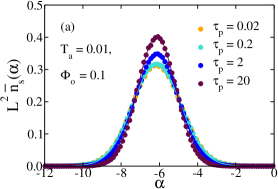
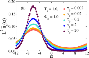
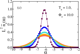
Figure 1: The tagged particle density distribution along the direction of the external potential, $L^{2}\bar{n}_{s}$, averaged over three different directions of the potential. (a) $T_{a}=0.01$, $\Phi_{0}=0.1$ and $\tau_{p}\in[0.02,20]$. (b) $T_{a}=1.0$, $\Phi_{0}=1.0$ and $\tau_{p}\in[0.002,20]$. (c) $T_{a}=1.0$, $\Phi_{0}=1.0$ and $\tau_{p}\in[0.002,20]$. Solid lines indicate Boltzmann distributions fitted to the data. The unperturbed distribution would be $L^{2}\times V^{-1}=L^{-1}=0.0407$.

For the external potential $\Phi$ varying along $\alpha$ axis, $\alpha=x,y,z$, the tagged particle distribution varies along the same direction and is uniform along the remaining two directions. In Fig. 1 we show tagged particle distributions averaged over the three directions of the perturbation. More precisely, we show $L^{2}\bar{n}_{s}(\alpha)$ where $L=24.56$ is the box size and the over-bar denotes averaging over three directions of the perturbation. We use the standard normalization condition $\int_{V}d\mathbf{r}\bar{n}_{s}(\mathbf{r})=1$. The distributions shown in Fig. 1 are significantly different from the tagged particle density in the absence of the external potential, when $L^{2}V^{-1}=1/L=0.0407$.

The important qualitative information that can be obtained from a quick look at Fig. 1 is that the tagged particle densities depend strongly on the persistence time of the self-propulsion.

To further verify that we are in the non-linear response regime in Fig. 2, we show the tagged particle mean squared displacements (MSDs) along the axis of the external potential (solid curves) compared to the mean squared displacement along an axis perpendicular to that of the external potential (dashed curves, for clarity shown for the longest persistence time only). We see that the MSDs along the axis of the external potential are significantly different from those along a perpendicular axis. In fact, for $T_{a}=0.01$ and $\Phi_{0}=0.1$ the tagged particle is localized at the external potential minimum on the time scale of the simulation.

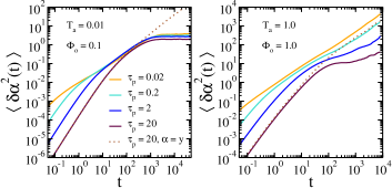
Figure 2: Tagged particle mean squared displacement along the direction of the external potential. (a) $T_{a}=0.01$, $\Phi_{0}=0.1$ and $\tau_{p}\in[0.02,20]$. Strong external potential leads to a localization of the tagged particle on the time scale of the simulation. (b) $T_{a}=1.0$, $\Phi_{0}=1.0$ and $\tau_{p}\in[0.02,20]$. Weaker external potential slows down the tagged particle motion but does not localize it on the time scale of the simulation. Dashed lines show tagged particle mean squared displacement in the direction perpendicular to the external potential for $\tau_{p}=20$. The motion in the perpendicular direction is unperturbed by the external potential.

The tagged particle density distributions shown in Fig. 1 can be fitted very well to the Boltzmann distribution $\propto\exp(-\Phi(\mathbf{r})/T^{\text{fit}})$ using $T^{\text{fit}}$ as the fit parameter commentfit . The resulting values $T^{\text{fit}}$ are shown in Fig. 3. We observe that the fitted temperatures decrease with increasing persistence time, which could have been anticipated from the persistence time dependence of the tagged particle densities.

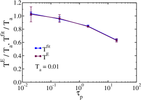
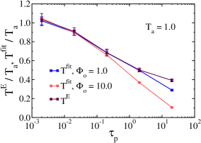
Figure 3: Comparison of the temperatures obtained from fitting Boltzmann distributions to tagged particle density distributions and the Einstein relation effective temperatures. (a) $T_{a}=0.01$, $\Phi_{0}=0.1$ and $\tau_{p}\in[0.02,20]$. (b) $T_{a}=1.0$, $\Phi_{0}=1.0$, and $\Phi_{0}=10.0$, and $\tau_{p}\in[0.002,20]$. All temperatures are shown relative to the active temperature $T_{a}$.

To verify our theory presented in Sec. II we need to check whether temperatures obtained from the fits, $T^{\text{fit}}$, are the same as the Einstein temperatures obtained from the ratios of the self-diffusion and tagged particle mobility coefficients. Even before calculating the latter temperatures we can infer from Fig. 3 that the theory does not work for the two longest persistence times for $T_{a}=1.0$. The reason is that the Einstein temperature describes an unperturbed system and thus does not depend on $\Phi_{0}$ whereas for the two longest persistence times for $T_{a}=1.0$ the temperatures obtained from the fits depend on $\Phi_{0}$. We will return to this issue at the end of this section.

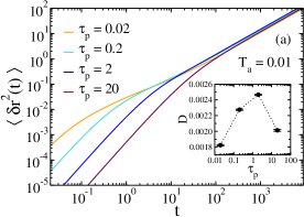
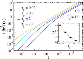
Figure 4: Mean squared displacement in unperturbed systems. (a) $T_{a}=0.01$ and $\tau_{p}\in[0.02,20]$. (b) $T_{a}=1.0$ and $\tau_{p}\in[0.02,20]$. Insets: persistence time dependence of the self-diffusion coefficient. $D$ is a non-monotonic function of $\tau_{p}$ at $T_{a}=0.01$ and decreases monotonically with increasing $\tau_{p}$ at $T_{a}=1.0$.

In Figs. 4(a-b) we show the MSDs $\left<\delta r^{2}(t)\right>$, where $\delta r^{2}(t)=\left(\mathbf{r}_{1}(t)-\mathbf{r}_{1}(0)\right)^{2}$, for unperturbed systems. The self-diffusion coefficients are calculated from these MSDs according to Eq. (35) and are presented in the insets. As anticipated and in agreement with earlier investigations FlennerSzamel2020 ; Berthier2017 , we get two different behaviors of the self diffusion coefficient at two active temperatures investigated. For the lower active temperature, $T_{a}=0.01$, we observe a non-monotonic dependence of the self-diffusion coefficient on the persistence time and for the higher active temperature, $T_{a}=1.0$, we observe that the self-diffusion coefficient decreases monotonically with increasing persistence time.

In Figs. 5(a-b) we show the persistence time dependence of the time-dependent response function $\chi(t)$ Szamel2017 at the two active temperatures investigated. The insets show the mobility coefficients calculated from the long time limit of $\chi(t)$ according to Eq. (36). We note that at the lower active temperature, $T_{\text{a}}=0.01$, the mobility monotonically increases with increasing $\tau_{p}$, in contrast to the non-monotonic behavior of the self-diffusion coefficient. At the higher active temperature, $T_{\text{a}}=1.0$, the mobility monotonically decreases with increasing persistence time, and thus exhibits the same $\tau_{p}$ dependence as the self-diffusion coefficient.

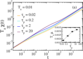
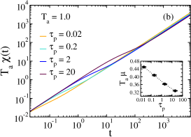
Figure 5: Time dependent response function to a weak external potential in unperturbed systems calculated using Eq. 37. (a) $T_{a}=0.01$ and $\tau_{p}\in[0.02,20]$. (b) $T_{a}=1.0$ and $\tau_{p}\in[0.02,20]$. Insets: persistence time dependence of the tagged particle mobility coefficient. $T_{a}\mu$ decreases monotonically with increasing $\tau_{p}$ at both active temperatures.

Comparing insets in Figs. 4(a-b) and in Figs. 5(a-b) we can see that at the smallest persistence times $D\approx T_{a}\mu$. This behavior is expected since in the limit of the vanishing persistence time at constant active temperature, the present model active systems become equivalent to Brownian systems at temperature equal to the active temperature, $T=T_{a}$. For a Brownian system the fluctuation-dissipation theorem holds and $D=T\mu$.

In Fig. 3 we compare the Einstein temperatures $T^{\text{E}}$ defined as the ratios $D/\mu$ to the temperatures obtained from fits to the Boltzmann distribution, $T^{\text{fit}}$. As mentioned in the previous paragraph, in the limit of small persistence times our active system becomes equivalent to the Brownian system and both $T^{\text{fit}}$ and $T^{\text{E}}$ become equal to the active temperature. With increasing persistence time, while keeping the active temperature constant, both $T^{\text{fit}}$ and $T^{\text{E}}$ decrease. We note that the decrease of the ratio of the Einstein temperature and the active temperature, $T^{\text{E}}/T_{a}$, was observed before Szamel2017 ; FlennerSzamel2020 . It contrasts with the increase of the ratio of the Einstein effective temperature to the bath temperature with increasing shear rate for colloidal suspensions under steady shear SzamelZhang2011 .

For the lower active temperature, $T_{a}=0.01$, we observe a very good agreement between $T^{\text{fit}}$ and $T^{\text{E}}$ for all persistence times investigated. In contrast, for the higher active temperature, $T_{a}=1.0$, we initially see a very good agreement between $T^{\text{fit}}$ and $T^{\text{E}}$ but then, for longer persistence times we observe that temperatures obtained from the fits deviate from the temperatures from the Einstein relation. Notably, it happens first for $T^{\text{fit}}$ obtained for the more confining potential, $\Phi_{0}=10.0$, and then $T^{\text{fit}}$ obtained for the less confining potential, $\Phi_{0}=1.0$.

We recall that our theoretical derivation in Sec. II relied upon the assumption that the spatial variation of the potential and of the tagged particle density occurs on the longest relevant length scale. On the other hand, we know that with increasing persistence time systems of self-propelled particles may undergo a motility-induced phase separation and that upon approaching such a transition they can exhibit long-range density fluctuations. To investigate the existence of such fluctuations we evaluated steady state structure factors of the unperturbed systems.

In Fig. 6 we show steady state structure factors $S(k)$,

$$S(k)=1+\frac{1}{N}\left<\sum_{i=1}^{N}\sum_{j\neq i}^{N}\exp\left[-i\mathbf{k}\cdot\left(\mathbf{r}_{i}-\mathbf{r}_{j}\right)\right]\right>,$$ (39)

for unperturbed systems at both active temperatures. We observe that for the lower active temperature, $T_{a}=0.01$, only a modest increase of $S(k)$ is observed for small wavevectors at the longest persistence times. This suggests that at this active temperature and in the range of the persistence times investigated density correlations are relatively short-ranged.

In contrast, for the higher active temperature, $T_{a}=1.0$, we observe a large small wavevector increase of $S(k)$ for the two longest persistence times. This suggests that at this active temperature at these persistence times there are long-ranged density fluctuations. To make this statement more quantitative we simulated a larger system consisting of $8\times 10^{4}$ particles at $\tau_{p}=2.0$. The small wavevector behavior of the steady state structure factor for this system is shown in the inset to Fig. 6. To quantify the range of the density correlations we fitted the numerical results to the Ornstein-Zernicke form $f(k)=a/[1+(bk)^{2}]$. We recall that parameter $b$ in the Ornstein-Zernicke fit is a measure of the density correlation length. We obtained $b=2.19$ which is perhaps moderate but is larger than the length on which the tagged particle density varies for $\Phi_{0}=10.0$ at $T_{a}=1.0$, $\tau_{p}=2.0$. Thus, in hindsight, it is not surprising that our theory is not applicable for these parameters.

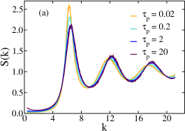
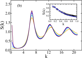
Figure 6: Stationary state structure factors of unperturbed systems. (a) $T_{a}=0.01$ and $\tau_{p}\in[0.02,20]$. (b) $T_{a}=1.0$ and $\tau_{p}\in[0.02,20]$. The upturn at small wavevectors indicates increasing correlation length. Inset in (b): small wavevector behavior of the structure factor calculated using $8\times 10^{4}$ particle system for $T_{\text{a}}=1.0$ and $\tau_{p}=2$. The solid line shows an Ornstein-Zernicke function, $f(k)=a/[1+(bk)^{2}]$, fitted to the data.

IV Conclusions

We derived an expression for the tagged particle density distribution in a slowly varying in space external potential in a system of interacting athermal active particles. The tagged particle distribution has the Boltzmann functional form, but the role of the temperature is played by the ratio of the self-diffusion and tagged particle mobility coefficients. We used computer simulations to verify the theoretical result. The theory works well if the characteristic length of the tagged particle density variation is the longest relevant length in the system. The theory is inapplicable if the characteristic length of the density fluctuations is longer than the the characteristic length of the tagged particle density variation.

The ratio of the self-diffusion and tagged particle mobility coefficients has long been known as the Einstein temperature, one of several effective temperatures obtained for non-equilibrium systems from the fluctuation-dissipation ratios. Our result shows that the Einstein temperature determines the large spatial scale tagged particle density distribution beyond the linear response regime. This resembles earlier results that established that the Einstein temperature plays similar role for a single Brownian particle in a tilted periodic potential and for a tagged particle in a colloidal suspension under steady shear flow. These three results obtained for very different systems suggest that the Einstein temperature may be generally relevant for the large spatial scale tagged particle density distribution in any stationary non-equilibrium system in which the large scale motion is diffusive.

References

- (1) D. Chandler, Introduction to Modern Statistical Mechanics, (Oxford, New York, 1987).
- (2) N.A. Clark and B.J. Ackerson, “Observation of the Coupling of Concentration Fluctuations to Steady-State Shear Flow”, Phys. Rev. Lett. 44, 1005, (1980).
- (3) S. Ramaswamy, “The Mechanics and Statistics of Active Matter”, Ann. Rev. Condens. Matter Phys. 1, 323 (2010).
- (4) T. Vicsek and A. Zafeiris, “Collective motion”, Phys. Rep. 517, 71 (2012).
- (5) M. C. Marchetti, J. F. Joanny, S. Ramaswamy, T. B. Liverpool, J. Prost, M. Rao, and R. A. Simha, “Hydrodynamics of soft active matter”, Rev. Mod. Phys. 85, 1143 (2013).
- (6) J. Elgeti, R.G. Winkler and G. Gompper, “Physics of microswimmers-single particle motion and collective behavior: a review”, Rep. Prog. Phys. 78 , 056601 (2015).
- (7) C. Bechinger, R. Di Leonardo, H. Löwen, C. Reichhardt, G. Volpe, and G. Volpe, Active particles in complex and crowded environments, Rev. Mod. Phys. 88, 045006 (2016).
- (8) D. Needleman and Z. Dogic, “Active matter at the interface between materials science and cell biology”, Nature Rev. Mat. 2, 17048 (2017).
- (9) S. Ramaswamy, “Active matter”, J. Stat. Mech. 054002 (2017).
- (10) T.F.F. Farage, P. Krinninger, and J.M. Brader, “Effective interactions in active Brownian suspensions”, Phys. Rev. E 91, 042310 (2015).
- (11) M. Rein and T. Speck, “Applicability of effective pair potentials for active Brownian particles”, Eur. Phys. J. E 39, 84 (2016).
- (12) C. Maggi, U.M.B. Marconi, N. Gnan, and R. Di Leonardo, “Multidimensional stationary probability distribution for interacting active particles”, Scientific Reports 5, 10742 (2015).
- (13) T.A. de Pirey, G. Lozano and F. van Wijland, “Active Hard Spheres in Infinitely Many Dimensions”, Phys. Rev. Lett. 123, 260602 (2019)
- (14) L. F. Cugliandolo, “The effective temperature”, J. Phys. A: Math. Theor. 44, 483001 (2011).
- (15) R. Kubo, “The fluctuation-dissipation theorem”, Rep. Prog. Phys. 29, 255 (1966).
- (16) U. M. B. Marconi, A. Puglisi, L. Rondoni, and A. Vulpiani, “Fluctuation-dissipation: response theory in statistical physics”, Phys. Rep. 461, 111 (2008).
- (17) L. F. Cugliandolo, J. Kurchan, and L. Peliti, “Energy flow, partial equilibration, and effective temperatures in systems with slow dynamics”, Phys. Rev. E 55, 3898 (1997).
- (18) L. Berthier and J.-L. Barrat, “Nonequilibrium dynamics and fluctuation-dissipation relation in a sheared fluid”, J. Chem. Phys. 116, 6228 (2002).
- (19) For a review see, e.g., A. Crisanti and F. Ritort, “Violation of the fluctuation-dissipation theorem in glassy systems: basic notions and the numerical evidence”, J. Phys. A: Math. Gen. 36, R181 (2003).
- (20) J.-L. Barrat and W. Kob, “Fluctuation-dissipation ratio in an aging Lennard- Jones glass”, EPL 46, 637 (1999).
- (21) For a review see, e.g., L. Leuzzi, “A stroll among effective temperatures in aging systems: Limits and perspectives”, J. Non-Cryst. Solids 355, 686 (2009).
- (22) D. Levis and L. Berthier, “From single-particle to collective effective temperatures in an active fluid of self-propelled particles”, EPL 111, 60006 (2015).
- (23) G. Szamel, “Evaluating linear response in active systems with no perturbing field”, EPL 117, 50010 (2017).
- (24) I. Petrelli, L. F. Cugliandolo, G. Gonnella, and A. Suma, “Effective temperatures in inhomogeneous passive and active bidimensional Brownian particle systems”, Phys. Rev. E 102, 012609 (2020).
- (25) See also D. Loi, S. Mossa, and L. F. Cugliandolo, “Effective temperature of active matter”, Phys. Rev. E 77, 051111 (2008), where a different effective temperature was used in an active matter investigation.
- (26) E. Flenner and G. Szamel, “Active matter: quantifying the departure from equilibrium”, Phys. Rev. E 102, 022607 (2020).
- (27) K. Hayashi and S.-i. Sasa, “Effective temperature in nonequilibrium steady states of Langevin systems with a tilted periodic potential”, Phys. Rev. E 69, 066119 (2004).
- (28) G. Szamel and M. Zhang, “Tagged particle in a sheared suspension: effective temperature determines density distribution in a slowly varying external potential beyond linear response”, EPL 96, 50007 (2011).
- (29) For a general introduction to Chapman-Enskog expansion, see, e.g., P. Résibois and M. de Leener, Classical Kinetic Theory of Fluids (Wiley, New York, 1977).
- (30) U. M. Titulaer, “A systematic solution procedure for the Fokker-Planck equation of a Brownian particle in the high-friction case”, Physica A 91, 321 (1978).
- (31) G. Szamel, “Self-propelled particle in an external potential: Existence of an effective temperature”, Phys. Rev E 90, 012111 (2014).
- (32) E. Fodor, C. Nardini, M. E. Cates, J. Tailleur, P. Visco, and F. van Wijland, “How Far from Equilibrium Is Active Matter?”, Phys. Rev. Lett. 117, 038103 (2016).
- (33) L. Berthier, E. Flenner and G. Szamel, “How active forces influence nonequilibrium glass transitions”, New J. Phys. 19 125006 (2017).
- (34) In practice, we fitted function using both and as independent fit parameters. We verified that the resulting fits were correctly normalized, i.e. that within error.
- (35) B. Abou and F. Gallet, “Probing a Nonequilibrium Einstein Relation in an Aging Colloidal Glass”, Phys. Rev. Lett. 93, 160603 (2004).
- (36) N. Pottier, “Out of equilibrium generalized Stokes–Einstein relation: determination of the effective temperature of an aging medium”, Physica A 345 472 (2005).