Uncertainty Maximization in Partially Observable Domains: A Cognitive Perspective

Abstract

Faced with an ever-increasing complexity of their domains of application, artificial learning agents are now able to scale up in their ability to process an overwhelming amount of data; However this comes at a cost of encoding and processing an increasing amount of redundant information. This work exploits the properties of learning systems, applied in partially observable domains, defined to selectively focus on the specific type of information that is more likely to express the causal interaction among the transitioning states of the environment. Experiments performed under a total of 32 different Atari game environments show that adaptive masking of the observation space based on the temporal difference displacement criterion enabled a significant improvement in convergence of temporal difference algorithms applied to partially observable Markov processes under identical reproducible settings.

1 Introduction

Recent rapid developments in reinforcement learning (RL) rely on the ability to perceive and process a great surge of information collected through the interaction with real or simulated environments. With the evolution of sophisticated artificial sensory apparatus began the collective quest to improve the predictability of surrounding world dynamics by increasing the shear amount of data collected from it. The data greedy approach worked and consequently gave rise to significant breakthroughs and applicability of deep reinforcement learning (DRL). More complex architectures of neural network function approximators coupled with the increase of computational power allowed temporal-difference RL algorithms to achieve super-human level control in problems that were designed for the complexity and scale of human cognition, such as Atari games [36], complex board games such as Go [51, 50, 63, 48] , and modern strategy games like Starcraft II [62].

The aforementioned breakthrough approaches worked in part because both artificial and biological learning systems rely on the premise that their environment will provide them with enough informational entropy to improve predictability, while supporting their predominant function: adaptation. This Darwinian attribute of learning is evident in biologically-inspired machine learning mechanisms such as RL in the way that artificial agents adapt to their environment by creating and updating a policy $\displaystyle\pi$ that would ultimately select actions according to the maximization of the expected reward in the long run [57]. The adaptation of a RL agent by learning can be seen as a process of reducing the inherent unpredictability or entropy of the constantly changing environment: as the agent learns, it becomes better at predicting the environment dynamics i.e. how the environment reacts to the actions performed upon it. The learned predictive power allows an agent to gradually select better actions, i.e., those that would yield higher returns or rewards [57]. In this adaptive view of the learning process an artificial agent is reducing its ”surprise”, or entropy, about its perception of the environment according to the free energy principle [23]. Artificial RL systems faced with zero entropy state space and zero entropy reinforcement function would make learning useless: no potential uncertainty to reduce means that the system cannot learn.

Collecting more data from the environment by DRL approaches means that the learning agent’s state space encompasses more of the external world unpredictability providing the learning algorithms with more entropy “fuel” for learning. However, in most real world cases the amount of data collected from the environment is not linearly proportional to the overall entropy it yields: increasing the amount of perceived data also increases the chance of encoding highly predictable and redundant data in the agent’s state representations. Since that same data needs to be fed back into the learning system through a limited bandwidth channel we can look at presented challenges as a communication problem.Thus, under a communication channel assumption in RL an artificial learning agent forms a limited capacity communication channel between its perception (sensory input) and machine learning algorithm itself. The communication channel assumption intrinsically brings an important notion of its optimization; This is exactly the problem that Claude Shannon and John Tukey tried to solve during their period at the Bell Labs which inevitably led to the cornerstone of the information theory: the famous work by Shannon [49]. The communication problem the two engineers faced in a nutshell is getting as much of information (Shannon’s bits) through a channel of limited capacity measured by Tukey’s bits. Theoretically the ideal communication case would be if the transferred information Shannon bits were equal to Tukeys: We would have used the full potential of the channels bandwidth.

In ML approaches, however, the optimization of the communication channel equates to using the channel spanning peception and learning algorithm in such a way that would be beneficial for the entire learning process.

The approach presented in this work addresses the issue of optimization of a limited bandwidth communication channel between the agent’s perception and its learning algorithm, asserting the importance of looking at the learning problem (artificial and biological) as essentially uncertainty greedy. This proposal is based on exploiting this inherent, natural, informational dependence, which represents a characteristic of all learning processes. Instead of increasing the channel’s bandwidth in our quest to better describe the environment (so increasing the state-space dimension) the goal of the proposed approach is to utilize the available channel in a way that would maximize its ability to efficiently transfer the uncertainty or entropy of the perceived environment. The proposal relies on the simple, yet effective, concept of temporal difference displacement(TDD) criterion for state space masking, able to perform a selective filtering of the sensed state portions based on the amount of transitional information it carries. TDD approach borrows motion detection techniques, usually used in eliminating temporal redundancy during video compression. Before using the transition $\displaystyle(s,a,r,s^{\prime})$ for the learning, based on the two transitional states ($\displaystyle s$ and $\displaystyle s^{\prime}$) TDD produces a binary matrix able to mask-out the non-transitional information contained in them. The TDD reduced states are then integrated into their specific transition forming an optimized reusable learning block experience carrying in-itself only temporally correlated information.

TDDM-based masking makes possible for agent’s learning experiences to include the information needed to represent distinctions among world states (i.e. transitional information), while eliminating the constant information, alleviating the overload of the learning algorithm approximation process.

The proposed selective, attentive focus thus inevitably creates partially observable spaces from the perspective of learning agents; It does so in such a way as so to improve their ability to discriminate among the world states based on their temporal relationships; this, in turn, supports for development of better policies by inducing much needed determinism into the system.

The experimental results reported in Section 6 show that the active state space masking according to the TDD assumption can significantly improve the convergence of the TD learning algorithms defined over a partially observable Markov process in a variety of complex and sensory demanding environments such as Atari games. However, the TDD as a broader concept can be applied to variety of other ML approaches relying on hidden-Markov processes for world modeling. The article is structured in an incremental way, with the two first sections providing the general context of looking at the problem in a specific way, therefore building up a foundation for the approach.

2 The big picture: getting the right context

2.1 The perception problem: finding the right sources of uncertainty

Looking at the nature of things through the lens of the free energy principle [23] imposes a duality: on one side we have a tendency of the universe, i.e., our environment, to achieve the state of least energy expenditure, which is a high entropy one (in both informational and thermodynamic way), and, on the other side, learning adaptive systems, both biological and artificial, that fight against to this natural tendency to disorder. This fundamental disposition for learning for adaptation was observed from low complexity biological forms such as worms [44] and even organisms with no nervous systems [10]. Evolving from the simpler forms, the majority of biological systems have ever since improved their sensory apparatus and started maximizing their potential by the development of mechanisms that enable them to better cope with the abundance of surrounding entropy. The solution was simple: focus on a finite subset of the environment and further evolve techniques to process data observed from it to exploit the full potential of the specific perception.

For example, in the animalia kingdom the organisms have evolved a strong preference for detecting electromagnetic waves as they proved beneficial in reducing the uncertainty about their immediate environment, which, in turn, provided them with the possibility of better adaptation. Focusing on a specific range of electromagnetic spectrum allowed the formation of a structure that that we now refer to as “eye”. Over time, the biological systems evolved many types of sensory apparatus, but none of them conveyed as much entropy as visual information: most of the physical reality does not necessarily make disturbances in the air we could detect, or emit chemical compounds, but reflect electromagnetic waves and, more importantly, in a variety of different ways. Sounds and smells just do not give the possibility to differentiate the properties of the environment to provide a high entropy sensory input, visuals do. This surge of entropy acquired by the newly founded ability to extract information from the visible light spectrum made a huge evolutionary leap in the Upper Paleolithic era [21]: the search to expand the domain of perception quickly became a search to improve its processing. Perception moved from a simple reactive collection of neurons existing even before early Cambrian era [39] to the highly complex processing of visual information that now happens in a human brain. Certainly, the human sensory apparatus also improved in the evolution, but the evolution of mechanisms that process the data it can produce had a major role in rising to the Upper Paleolithic evolutionary boom [21]. The crucial ingredient was there, making sense of it was another issue.

2.2 The Quest for Complete Control

From a biological perspective [14] the function of learning as a reduction of uncertainty is to ensure the survival of a specific organism, its fitness to the environment. This enables it to choose the most adequate set of possible actions for any given situation, while effectively avoiding the risks of blindly trying out an action that could be fatal. The process of uncertainty reduction in a dynamic environment provides a constant goal-directed drive for evolutionary behaviour.

The early cybernetic work of [5, 20] views the goal of survival in a dynamic environment strictly as a control problem, in which the control is exerted by compensating for dynamic perturbations that make the system deviate from its goal: maintaining or increasing its fitness.

If we consider survival as a primary evolutionary goal, mediated by the agent’s ability to adapt to a constantly changing environment as a strict Ashby’s type control problem, we could be bound to Ashby’s Law of Requisite Variety ([20]): For an organism to converge to an optimal evolutionary goal or complete control, in Ashby’s view the variety of compensatory actions that its control system is capable to execute must be able to cope with the perturbations that might occur in its environment.

However, moving from a simplified control perspective, an adaptive learning system mediates this quest for complete control by creating and constantly updating a model of the objective environment. The infinite variety of all possible perturbations of the simple Ashby’s type of system are now mapped onto a finite set of action-triggering representations: its state space.

An artificial learning agent moves from the one-to-one perturbation-action assumption of ([20]) to a many-to-many type of a relationship between finite sets of state and action pairs. The evolutionary-driven fitness realization shifts from a simple reactive compensatory role to a much demanding long-term survival-supporting role of forming effective internal representations capable of effectively representing the features that are relevant to the agent’s goal. The focus on agent perception ability within the machine learning community began mostly with the introduction of perceptual aliasing term by [66, 67] which would be later incorporated in the wider concept of active perception.

An actively perceiving artificial learning agent capable of effectively conveying the variety and importance of possible perturbations of the system through its internal representations while sustaining its discriminatory ability is capable of producing action polices that can exert an adequate amount of control for the agent to be able to achieve its goal of adaptation. This work, under the communication channel assumption, explores how and to which extent artificial learning agents can maximize the potential of their internal representations to deliver the information that would be most supportive for the learning goals.

2.3 Not all entropy is useful: a qualitative perspective on information

Life’s quest for a reduction of uncertainty (as far as we know) didn’t appear in high energy environments such as the gas giants of our Solar system, nor did it sustain in the low energy ones such as the Earth’s Moon or Mars, for example.

This biological process, however, has some prerequisites in terms of the amount of dynamic perturbations of an environment: they need to be just enough to enable to predict the patterns of causal relationships between the changing states according to the integrated information principle [59] focusing on the dynamic environmental processes that have a causal influence on the system’s goal.

The integrated information $\displaystyle\Phi$ represents the information that is irreducible to its non-interdependent subsets, which, in our case, are the representations of the environmental states. Instead, this type of information explains the relationships between them, supporting the integration of a set of phenomenal distinctions into a unitary experience [59].

The ability of a learning system to extract the information from its environment depends on the amount causal, different perturbations found in that environment which are meaningful to its learning goal. This selective process can again be viewed as a direct optimization of the agents’ communication channel between its perceptual and learning system.

A constantly varying and high-entropy environment, as a prerequisite for an evolutionary drive, entails an organism capable of not only mapping static environment objects to their representations, but also dynamic perturbations of the environment (such as temporal correlations) to its own actions.

The preference for cognitively mapping the environment dynamics that exhibits temporal correlations, rather than its static equilibrium states has been predominantly observed in insects perceptual mechanisms  [45, 28, 55]. The focus on the dynamic perturbations of the environment by the way of motion flow detection in honeybees [55] and locusts [52] is essential for mediating their flight steering maneuvers and escape jumps in response to a looming threats.

The well known Goldilocks [43] thermodynamics property of habitable planets can be extended in the Shannon’s sense as the optimal informational saturation condition of all learning systems, biological and artificial.

Thus, a more perceptually efficient agent could, under the communication channel assumption, mediate and alias the perception to a greater extent, while optimizing its communication channel, effectively allowing the learning system itself to focus on a more ”useful” information (i.e. the information carrying more of the environments’ dynamic perturbations [59]).

Under cognitive perspective the efficacy of learning not only depends on the level of environment entropy, but also on the amount of the entropy that can be perceived or channeled to the learning system itself. This property provides a basis and has been heavily exploited under the communication channel assumption introduced in Section 1

2.4 Learning to live with uncertainty (and learn from it)

The breakthroughs in artificial learning algorithms mentioned in Section 1 have dealt with the uncertainty of the world by focusing on the part of it that was deterministic in nature and defining it as a Markov Decision Process (MDP) [57]. This represented a sort of a leap of faith as most of real-world problems are inherently non-Markovian: the world itself is highly non-Markovian, and complex biological learning systems like humans have benefited from this as suggested in Section 2.1. Even though, since the mid 60ies the artificial intelligence community have developed methods that could represent and reason with uncertainty that originate from the control engineering perspective of Karl Johan Åström [6]. The majority of TD methods have relied on this deterministic safe haven of MPDs. This tendency could be partially attributed to the fact that the proofs of the convergence of TD algorithms assumed the agent’s perceived state space to be Markovian and ergodic in nature [64, 60]. Despite the convergence issues the artificial intelligence community adopted a non-deterministic method as a (more or less) natural extension of MDP under the name of partially observable Markov decision process or POMDP [38, 32, 15].

2.5 Extending the MDP

A Markov Decision Process is fully defined by the tuple $\displaystyle\langle S,A,T,R\rangle$, which includes: a finite set of environment representations S that can be reliably encoded by the agent, a finite number of actions A that an agent is allowed to perform in that environment, a transitional model of the environment T providing a functional mapping of $\displaystyle S\times A$ to discrete probabilities defined over $\displaystyle S$, and a reward function $\displaystyle R(s,a)$ which maps the state and action pairs from $\displaystyle S$ and $\displaystyle A$ to a scalar indicating the immediate reward feedback the agent receives from being in a specific state $\displaystyle s$ and taking a specific action $\displaystyle a$ [57]. In POMDP’s the algorithm doesn’t have the benefit of performing the mappings of $\displaystyle S\times A$ over a set of deterministic states $\displaystyle S$ but rather on a set of the possible partial observations O of the states [15]. In other words, the additional modelling of the concept of observation was required. The solution for this problem came in the form of a belief state: an internal representation that maps the environment states to the probability that the environment is actually in that state. The belief state denoted by $\displaystyle B$ is simply a probability distribution that can be represented by a vector of probabilities, one for each possible state of the environment, summing to 1 [15]. This articulates the problem of learning in a partially observable environment as a problem of estimating the ”true” state of the world based on the belief state derived from the agent’s partial observations.

The POMDP agent improves its estimates of the model of the environment by updating its state estimate $\displaystyle\tau(b,a,o,s^{\prime})$ about the state $\displaystyle s^{\prime}$ based on the previous belief state $\displaystyle s$ along with the most recent action $\displaystyle a$ and the most recent partial observation $\displaystyle o$ by applying the simplicity of the Bayes’ rule according to Equation 1. Transitional probabilities $\displaystyle\tau(s,a,s^{\prime})$ in Equation 1 are given as in vanilla MDP’s and $\displaystyle b(s)$ represents the actual probability that is assigned to the state $\displaystyle s$ considering an agent being in a specific belief state $\displaystyle b$.

$$\begin{split}\tau(b,a,o,s^{\prime})&=P(s^{\prime}|a,o,b)\\ &=\frac{P(o|s^{\prime},a,b)P(s^{\prime}|a,b)}{P(o|a,b)}\\ &=\frac{O(s^{\prime},a,o)\sum_{s\in S}\tau(s,a,s^{\prime})b(s)}{P(o|a,b)}\end{split}$$ (1)

Regardless of their differences, solving problems defined over MDP and POMDP come down to finding a policy $\displaystyle\pi$ that will maximize the future expected reward [57]. While in the case of MDP this policy represents a mapping of deterministic states $\displaystyle S$ to actions, in POMDP the actions are chosen based on the basis of the agent’s current belief states $\displaystyle b$. Along the iterative update of the agent’s belief state using Equation 1 the agent’s first step towards learning a policy $\displaystyle\pi$ is the iterative update of the value functions $\displaystyle V$ for each of its belief states using dynamic programming methods [9] such as value iteration outlined in Equation 2 (this is where the inherent complexity of the POMDP approach becomes apparent). The updated value function $\displaystyle V_{n+1}$ in Equation 2 is calculated on the basis of the previous value function $\displaystyle V_{n}$ defined over the current state estimate given by Equation 1 and immediate expected reward $\displaystyle r(b,a)$ of executing action $\displaystyle a$ in belief $\displaystyle b$. The expectation of this scalar reward $\displaystyle r(b,a)$ is based on the whole state space and the current belief $\displaystyle b(s)$ as defined in Equation 3.

$$V_{n+1}(b)=\max_{a}\left[r(b,a)+\gamma\sum_{o\in O}P(o|b,a)V_{n}(\tau(b,a,o))\right]\forall b\in B$$ (2)

$$r(b,a)=\sum_{s\in S}b(s)r(s,a)$$ (3)

For an arbitrary value function $\displaystyle V$ updated by Equation 2, a policy $\displaystyle\pi$ is said to be actually improving on V under the Equation 4 . The convergence of the policy $\displaystyle\pi$ to the optimal policy $\displaystyle\pi^{*}$ is the result of the value function $\displaystyle V$ convergence to $\displaystyle V^{*}$ as the number of iterations $\displaystyle n$ goes to infinity.

$$\pi(b)=\arg\!\max_{a}\left[r(b,a)+\gamma\sum_{o\in O}P(o|b,a)V(\tau(b,a,o))\right]\forall b\in B$$ (4)

If we simply omit the $\displaystyle\max_{a}$ operator from Equation 2 we get a representation of the value of executing a specific action $\displaystyle a$ in a current belief state $\displaystyle b(s)$. This representation, also known as Q-value, is given in Equation 5 and its is widely used in temporal-difference learning since Watkins’ paper [64].

$$Q_{n+1}(b,a)=\left[r(b,a)+\gamma\sum_{o\in O}P(o|b,a)V_{n}(\tau(b,a,o))\right]\forall b\in B$$ (5)

2.6 POMDP as state-of-the-art

However, solving a problem defined over POMDP proved not to be such an easy task due to the complexity [46, 30] imposed by a creation of a belief state $\displaystyle B$ that, in most of the cases, has the same dimension as $\displaystyle|S|$: the dimension of the belief space thus grows exponentially with $\displaystyle|S|$. A certain revival for POMDP’s, though, came with the introduction of more complex function approximators: for most non-trivial cases keeping track of the values $\displaystyle V$ given by Equation 2 for each of the observations was computationally unfeasible because of their sheer numbers, and for this reason the value functions have been approximated by ANN ranging back to Lin [31]. The approximation is done by nudging the parameters or weights $\displaystyle\Theta$ of an ANN by a small learning rate $\displaystyle\alpha$ at each learning step so that the current estimate $\displaystyle Q(b,a;\Theta)$ will be closer to the target Q-value given by Equation 5. This is done by minimizing the loss function $\displaystyle L(\Theta)$ representing the difference between the previous estimate and the expectation target by performing a stochastic gradient descent on the weights $\displaystyle\Theta$ to achieve $\displaystyle Q(s,a;\Theta)\approx Q^{*}(s,a)$ according to Equation 6:

$$\nabla_{\Theta_{i}}L_{i}(\Theta_{i})=\left(y_{i}-Q(b,a;\Theta_{i})\right)\nabla_{\Theta_{i}}Q(b,a;\Theta_{i}),$$ (6)

where $\displaystyle y_{i}$ represents our target Q-value obtained by calculating the Bellman optimality under the newly observed transition parameters over Equation 5.

Later, the introduction of many-layered deep ANN’s capable of scaling up to an over-increasing sensory demand of modern RL applications [36, 37, 51, 50, 62, 63, 48] inspired deep learning POMDP approaches by Hausknecht and Stone [24] and, more recently, by Le [29]. Their deep recurrent Q-network (DRQN) achieved a better adaptation of agents under the circumstances where the quality of observation changes over time compared to vanilla DQN. Because of its appoximation power and scalability over the POMDP domain the DRQN approach is used as a basis for the proposed TDDM filtering architecture further elaborated in Section 4.

3 POMP as Perception Mechanism

Why would we link perception to partially observable Markov decision processes? The nature of perception itself lies in selective filtering, processing, redefining, and, in most cases, interpreting the raw data received through an agent’s sensory apparatus.

An agent is not acting upon the idealized full potential of the informational content present in its immediate environment, but on a small subset of processed observations, which are often moved to latent spaces. Despite of this limitation, the biological agents may act optimally in a partially observable world by building something that could be seen as POMDP belief states.

3.1 Pioneering approaches

One of the first computational perspectives on perception was concerned about its most dominant and entropy rich modality: vision as formulated in the late 70ies by David Marr [33, 34]. These works postulate a theory of early visual computational processing that has inspired some of the pioneering works [3, 2] dealing with the problem of computational perception as an important component of artificial learning agents. Marr’s work set a theoretical base for the principle of what Agre and Chapman called deictic representation by postulating that the first operation on a perceived raw image is to transform it into a more simple, but entropy rich, description of the way its intensities change over the visual field, as opposed to a description of the intensities themselves [33, 34]. This primal sketch, as he coined it, provides a description of significantly reduced size that is still able to preserve the important information required for image analysis. The importance of the Agre and Chapman deictic approach [3, 2] from the perspective of the here proposed work lies in its architecture: the crisp distinction between the perception system and the central system (i.e. the learning algorithm). The visual system thus takes the deictic burden: at any given moment, the agent’s representation should actively register only the features or information that are relevant to the goal and ignore the rest. This architectural modularity allows the central system in [3, 2] to be implemented in a rather simple way without the complexity of a pattern matcher or similiar computationaly demanding processes; the deictic process enables generalization over functionally and indexically identical states of the environment by simply not bringing in the redundant distinctions among them.

Later work of Ballard et. al [8, 25] put the deictic principle of [3, 2] into the broad context of visual processing of biological systems suggesting that the human visual representations are limited and task dependent. [8, 25] further postulate that the superior human performance in visual perception can be attributed to the sequence of constraining deictic processes based on a limited amount of primitive operations supporting the notion that a human working memory is limited in its capacity and computational processing ability [12, 7, 47].

A more complex extension of [3, 2] is given by Chapman [17] through their SIVS architecture. SIVS have introduced a selective deictic visual processing of subsets of an image by identifying the regions that are ”task dependent”. The interesting part of the SIVS approach is that it implements, amongst other, a concept of visual routines inspired by [61], which actively process the visual information within the time-domain, allowing for the detection and abstraction of changes in the visual field [17]. The Chapman’s applications of the visual routines is very much in line with the temporal context retaining properties of POMDP-based learning algorithms presented in this work.

3.2 Getting the Problem Right

The deictic way of looking at a machine learning problem seemed very promising because of its ability to represent as equivalent the world states that require the same action according to the agent’s current policy: more abstracted, more compacted representations reduce the burden on learning mechanisms. As the researches eagerly exploit the possibilities of modeling artificial perception under the deictic principle a concern arises whether this selective, compact, and task-dependent world representation can be acted upon deterministically with respect to the Markov property in order for an agent to achieve optimal policy [67, 19]. The integration of adaptive control methods such as active perception with the machine learning algorithms [64] may lead to a phenomenon of perception aliasing [67] as it can produce internal representations that are not consistent with each other.

Lack of consistency among states can be very detrimental to the TD algorithms [64] as their underlying principle of Bellman’s optimality [9, 57] relies on this property: inconsistent states can destabilize the learning algorithm by introducing unfounded maximums in the value function [67] which, in turn, can make the agent diverge from its optimal policy. Furthermore, perceptual aliasing can lead to distinct world states that may call for equally distinct actions according to the optimal policy being represented by the same deictic representation.

3.3 Correlation Saves the Day

A partial solution was readily proposed by the work that introduced the problem of perceptual aliasing [67] in the first place and it was based on detecting and suppressing the representations that are less correlated. As the MDP assumption still relied on the deterministic principles the correlation between the states in [67] seemed to be a part of the system that was the source of certainty.

The here presented work extends that notion in the direction of the work by [18] that used the memory of the previous states in order to detect the essential information that can induce correlations. In this case, the previously experienced correlations among the states are used to build a probabilistic model that is able to predict the current world state. Although probabilistic models have been used in reinforcement learning as a form of experience replay [56, 31] the so-called predictive distinctions approach of Chrisman [18] used it to drop the deterministic assumptions of the agent’s representations by implementing a Hidden Markov Model (HMM) [41]. Proposing the powerful, yet (at the time) untapped predictive ability of RNN’s [27] to extend the Chrisman’s approach led to artificial agents with a better grasp of uncertainty which, in turn, led to the definition of POMDP.

McCallum [35] used a similar HMM approach, so-called utile distinction memory, introducing the possibility of discriminating states based on their perceived utility: the world states represented by the identical observations could be distinguished based on their prior assignments of rewards thus driving the system ability to discern the states. The utile distinction memory [35] approach raised a possibility for further optimizations of the memory process itself as seen in the later work by Wiestra and Weiring [68] on utile distinction hidden Markov models or UDHMM. We can relate the UDHMM approach to the here presented work as it too optimizes the learning process by limiting the amount of the informational entropy being channeled to the learning algorithm in such a way that distinctions of the specific world states would be represented in memory only when needed.

While the UDHMM does this by adjusting the number of steps it looks back in order to create the utility distinctions, the approach proposed in this work rather focuses on isolating a subset of the observations that induce the distinction-relevant information while ignoring the extraneous part. This observation partitioning principle has been successfully implemented in a class of POMDP’s called mixed observability Markov decision process or MOMDP introduced by Ong et al. [40]. MOMDP exploits the fact that although the agent perceives limited representations of the world, some subset of its observations can be deterministic in the sense that they possess a fully observable property. In MOMDP approach the agent state is split into the fully observable component $\displaystyle x$ and the partially observable one $\displaystyle y$ which leads to the computational benefits of maintaining and updating a belief state $\displaystyle b_{y}$ about the $\displaystyle y$ component only.

The aforementioned improvements of the base algorithm bring the focus on the problem of artificial perception [65, 53] as a way for an agent to intrinsically and dynamically learn what to perceive in the first place. One of popular approaches to active perception defined over POMDP includes designing a reinforcement function in such a way that it would minimize the sensing cost [11], minimize the agent’s belief state uncertainty based on its current measure of entropy [4], or credit the belief level achieved by the specific sensed state [54].

To mitigate the effects of encoding a great amount of low-entropy data that does not support the learning process, the recent approaches prioritized on the agent’s experiences that carried more entropy [42] or used an array of unsupervised learning techniques in order to compress the world representations into vectors with high entropy [62]. Both approaches were effectively conveying more of the environment’s uncertainty to the learning agent itself, improving the learning performance.

More recent work [69] relates observations with the agent’s actions by encoding them together in such a way that the LSTM layer can propagate the additional context of actions through the history of observation-action pairs. In [16], ANN function approximators are used to split the sensory input in the partially observable subset that is included in the POMDP’s history of the past states and the fully observable subset that is treated as Markovian.

Artificial attention has been explored recently in the context of standard MDP-based reinforcement learning problems through evolutionary techniques, taking biological inspirations such as intentional blanking in the approach by Tang et. al. [58].

4 Model Architecture and Theoretical Background

This work introduces a novel method of improving the propagation of environment’s inherent uncertainty or entropy to the temporal-difference reinforcement learning algorithm defined over a partially observable domain by introducing a perceptual aliasing method of the agent’s state space based on the concept of temporal difference displacement criterion or TDD. The TDD perceptual aliasing acts by optimizing the communication channel established between perception and the learning mechanism in such a way as to transfer as much of the environments dynamic perturbations, or causal information [59] possible given the channels limited bandwidth.

The TDD criterion as perceptual aliasing mechanism selects the information perceived by the agent, so that the information which does not contain learning potential (as defined by the communication channel assumption presented in Section 2.3) will not be transferred to the learning algorithm.

The proposed TDD criterion exploits the following properties of these types of learning algorithms:

• By each successive TD transition the algorithm takes advantage of the temporal relations between the transitioning states in order to improve its belief state about the environment: the policies that an agent develops are not a product of deterministic states, but are based on the history of (possibly) all previous observations and their underlying relationships.

• The POMDP agent still updates its policy based on a single transition from state $\displaystyle s$ to state $\displaystyle s^{\prime}$ by performing an action $\displaystyle a$: this one step information along with a reward scalar constitutes everything the algorithm needs in order to perform a learning update [64].

Moreover, the TDD criterion postulates the following:

• Each of the two subsequent states ($\displaystyle s$ and $\displaystyle s^{\prime}$) in a single learning transition can either have a positive or negative effect on the uncertainty reduction of the belief state, based on their temporal relationship [15].

• The modification between subsequent observation states ($\displaystyle s$ and $\displaystyle s^{\prime}$) that a specific transition has induced is as relevant to reduce uncertainty about the agent’s belief state as its informational content supports the ability to distinguish states from each other.

• The changes in the observation states ($\displaystyle s$ and $\displaystyle s^{\prime}$) channel a lot of the environment uncertainty or entropy required for creating an accurate observation model: they carry the highly valuable information about the transitional relationships.

• For the intuition regarding the previous paragraph let us imagine a case in which all of the observations were exactly the same but the transitions yield different rewards. The POMDP learning algorithm would try to attribute the reward differences to the states in the form of value functions, but there would not be learning because the states would be indistinguishable from each other ($\displaystyle s=s^{\prime}$).

In other words TDD provides a simple yet effective way to maximize the amount of informational entropy that is dedicated to the representation of causal relationship between the environment states or states representations according to the integrated information principle [59].

The full potential of the TDD perspective on learning is realized through an active state space masking or selective filtering of the agent’s observations based on the temporal difference displacement between the initial perceived state $\displaystyle s$ and its successor $\displaystyle s^{\prime}$. Figure 1 details the applied TDD transformations to an Atari game learning problem example.

In the visual channel used in the examples on which we tested the systemd, the TDD criterion is estimated with a computationally inexpensive two-frame motion estimation technique based on polynomial expansion [22] capable of producing a dense optical flow vector field based on two successive video frames, which, in the case of TDD includes observation states of the agent’s atomic transition ($\displaystyle s$ and $\displaystyle s^{\prime}$) as detailed in Figure 1.

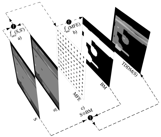
Figure 1: The process of active state masking based on TDD decomposed with regards to its functional transformations $\displaystyle f$ represented by black circles; a) motion estimation based on polynomial expansion [22]; b) Binary threshold mask generated from the motion-field vector magnitudes obtained from a); c) Element-wise matrix multiplication of the original frame S with the binary mask obtained from b).

After the initial problem-specific prepossessing of perceived visual information, the two successive frames, namely, $\displaystyle S$ and $\displaystyle S^{\prime}$ are used as an input for the motion field estimation function $\displaystyle f_{MFE}$ in Figure 1 $\displaystyle a)$.

In order to perform the motion estimation $\displaystyle f_{MFE}$ function analyses the displacement of the intensities (dx,dy) between the starting image $\displaystyle I(x,y,t)$ at the time $\displaystyle t$ and image $\displaystyle I(x+dx,y+dy,t+dt)$ that is obtained after temporal displacement $\displaystyle t+dt$.

The initial displacement analysis [22] produces a dense motion field estimate window or MFE (see Figure 1) commonly depicted by using oriented Cartesian vectors representing the intensity and direction of detected temporal displacements.

The obtained dense motion field is then transformed to a binary threshold mask or BM in Figure 1 by applying a simple adaptive high-pass filter on the magnitude component of the vector.

Each transition generates its own unique binary mask BM which is multiplied element-wise with each state input in Figure 1c) effectively performing TDD masking $\displaystyle TDDM(S)$ on the input prior to its integration into the main TD learning algorithm.

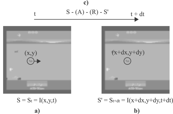
Figure 2: Simplified process of motion estimation based on the amount of displacement $\displaystyle(dx,dy)$ detected between two transitional states of an Atari game example. The common Atari preprocessing includes resizing the input to a 84x84 matrix and reducing three color channels to a single grayscale one; a) Image intensity $\displaystyle I(x,y,t)$ at time $\displaystyle t$ or $\displaystyle S_{t}$; b) Image intensity $\displaystyle I(x+dx,y+dy,t+dt)$ after a $\displaystyle dt$ amount of time has passed or $\displaystyle S_{t+dt}$; c) During the $\displaystyle dt$ time-window the autonomous agent has successfully performed a transition defined over a MDP by taking an action $\displaystyle(A)$, obtaining immediate reward $\displaystyle(R)$ and observing $\displaystyle S_{t+dt}$ state at the final time of $\displaystyle t+dt$.

Figure 3 outlines the final component of main learning part of the algorithm: Q-value approximation using three layers of convolutions [24] together with the proposed $\displaystyle TDDM$ component processing the input.

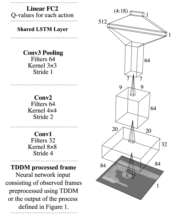
Figure 3: The final Q-value approximating component combining active state masking with three convolutional layers, a LSTM layer connected with $\displaystyle n-1$ sequence of previous ones and a linear fully connected one at the output. The example input is defined as a TDDM processed Atari game frame.

The recurrent property of the LSTM component [26] applied just before the output layer in Figure 3 is responsible for processing activations through time allowing the ANN to infer on the transitional information from the past states. This context of previous states and actions is crucial in leaning algorithms defined over POMDP, as it provides a way to disambiguate the states of the environment. In order to achieve this, LSTM layer shown in Figure 3 recurrently connects with the $\displaystyle n$ LSTM layers that process $\displaystyle n$ previous agent’s states. The presentation of the architecture of a LSTM is out of the scope of this work; we only mention that the basic working principle behind it is a recurrent neural network propagation of a hidden state $\displaystyle H$ through the layers.

To appreciate the contribution of the LSTM recurrence to the overall architecture, we observe a less complex RNN architecture showcased in Figure 4. Let’s say that we want to base the agent’s decision making (in our case, the approximated Q-value) not only on current perceived state, but on the $\displaystyle n$ previous ones, $\displaystyle S_{t}$ being the current one and $\displaystyle S_{t-n}$ the oldest one in our horizon. From Figure 4 it is clear that $\displaystyle n$ layers are implemented, each receiving their respective temporal input $\displaystyle(x_{n}$ to $\displaystyle x_{0})$, but at the same time each of them generating an internal hidden state H at the output, which becomes a part of the next layer input, thus propagating the context of the $\displaystyle n$ states. By viewing the main architecture in this recurrent perspective it is clear that Figure 3 shows only the last network out of $\displaystyle n$ identical ones, each being interconnected with their LSTM layers for essential recurrence property. The outlined last layer is used to approximate the final Q-values from the outputs of the last LSTM layer but its approximations are a product of recurrent context transfer through the previous $\displaystyle n-1$ LSTM layers.

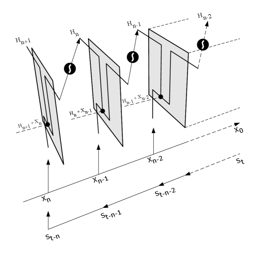
Figure 4: The hidden state propagation of a basic recurrent neural network architecture. The inputs of the gray layers are denoted as $\displaystyle X$, agent’s states are denoted as $\displaystyle S$, and hidden states by $\displaystyle H$. The big black circle represents the activation function applied to the layer’s output, while the small one represents the concatenation operator.

5 Experimental Setup

The TDD proof-of-concept evaluations were performed on a variety of Atari games environments on a Python based platform mainly supported by Tensorflow [1] and OpenAI Gym [13] frameworks with all of the aspects of the architecture and setup being based on the vanilla DRQN approach originally presented by Hausknecht et al. [24]. Due to their complexity and visual variety Atari games as a set of learning problems were adopted by the original DRQN paper [24], we are also doing the same in our benchmarks. However, TDD masking approach is not limited to the information that is represented in a spatial and visual way as in Atari learning problems: The temporal difference displacement concept can be applied for selective masking of any state representations, for example a different extreme would be a flat one-dimensional vector state of a simple CartPole problem [57].

The purpose of the evaluation was to compare the learning performance of the baseline DRQN [24] with DRQN-TDDM, an implementation that extends the baseline to include the proposed active state masking based on the TDDM criterion. The DRQN and DRQN-TDDM implementations share the same architecture and meta-parameters; their approximator weights and biases were randomly initialized. DRQN-TDDM only differs in its implementation of perceptual filtering based on a sparse TDDM mask that is multiplied element-wise with the corresponding observations before forwarding them as an input to the learning algorithm.

Agent’s policies were evaluated by performing $\displaystyle 5$ independent learning trials for each of the two systems (DRQN and DRQN-TDDM) and averaging their achieved scores. An ANN function approximator shown in Figure 3 was trained on each trial for a total of 7 million iterations with a root mean square propagation (RMSProp) optimizer capable of decaying the initial learning rate $\displaystyle\alpha=0.00025$ by a decay rate of $\displaystyle 0.97$. The RMSProp also implemented a momentum of $\displaystyle 0.95$ and additional gradient clipping. At each iteration the ANN’s training data included a mini-batch of $\displaystyle 64$ transitions uniformly sampled from a sliding-window replay memory of size $\displaystyle 800.000$. Agent’s action selection was mediated by an adjusted $\displaystyle\epsilon-greedy$ approach; the starting $\displaystyle\epsilon=1.0$ was decayed gradually during the learning process to a final $\displaystyle\epsilon=0.01$. The decay process started after the first million steps and proceeded linearly afterwards. The discount factor $\displaystyle\gamma$, a parameter of the Bellman’s Equation 5 was set to a high value ($\displaystyle 0.99$).

6 Experimental Results

The results for the evaluation phase compared the learned Q-network parameters obtained in the Training phase under identical configurations. During this stage the network parameters obtained by the baseline and by $\displaystyle TDDM$ filtering were both evaluated with an original state input, providing a robust $\displaystyle TDDM$ benchmark.

The evaluation benchmark consisted of a reproducible batch of 10 independent act-only trials for each of the ANN models obtained during the training phase. An act-only trial is characterized by acting upon the learned policy with no random exploration actions taken ($\displaystyle\epsilon=0$).

Each of the independent evaluation trials were performed for a total of 100,000 steps on an original unfiltered Atari input. To guarantee reproducibility of the evaluation results a vector of 10 random scalars was generated a-priori, specific to each game. The unique scalars have been used to seed the pseudo-random number generators of all the relevant frameworks governing the behaviour of the Atari emulator, making it deterministic with respect to the scalar used.

Faced with the identical and reproducible conditions the ANN models trained under $\displaystyle TDDM$ filtering outperformed the baseline ones in 20 of a total of 32 Atari game environments evaluated under the benchmark. This is reported in Table 6. The general performance measure is defined as the average return or reward that an agent received during its 10 independent batch trials; this measure represents the quantity reported along the $\displaystyle A.R.$ or Average Reward, column of Table 6. Table 6 outlines the summary of the performed benchmarks with the best performing values under each Atari-environment being highlighted in bold. Each row of Table 6 represents an independent benchmark batch. Each game environment is represented by a total of two trial batches: the $\displaystyle TDDM$ and the baseline. The batches performed with the $\displaystyle TDDM$ models have been highlighted with a light gray background.

The obtained $\displaystyle TDDM$ masking ratios/amounts indicated in Figure 6 a) show a very strong preference of TDDM trained models (in orange) for states that would be masked to a higher degree compared to the baseline (blue) in which this bias is not present. The discriminatory ability of $\displaystyle TDDM$ models can be also appreciated from the visual comparison of the masking dynamics of the best performing games in Figure 5; Contrary to their baseline counterparts, the models trained using $\displaystyle TDDM$ are characterized by a much higher degree of masking, effectively removing more of the non-temporally-correlated data. Because of the $\displaystyle TDDM$ models ability to discriminate, the agents using $\displaystyle TDDM$ trained models display an artificial attention that is closer to focused attention.

For most of the evaluated games, it can be noticed that the ability of the $\displaystyle TDDM$ filter to discriminate between the two categories of information directly affects the performance of the $\displaystyle TDDM$ trained models. The cases where $\displaystyle TDDM$ models haven’t outperformed their baseline include games that are characterised by a high amount of flickering such as DemonAttack-v0,Time-pilot-v0,Poenix-v0 and games with a high amount of repetitive synchronized movement sources such as Freeway-v0,SpaceInvaders-v0. The low performing $\displaystyle TDDM$ examples as shown in the right column of Figure 5 held a specific set of characteristics (not limited to the above-mentioned ones) which were detrimental to the two-frame dense optical flow [22] detection accuracy and more importantly its discriminatory ability.

Although no TDDM masking was performed during the evaluation benchmark, the binary masks $\displaystyle BM$ were generated for analytical purposes using the identical TDD process, and are reported in Figure 1.

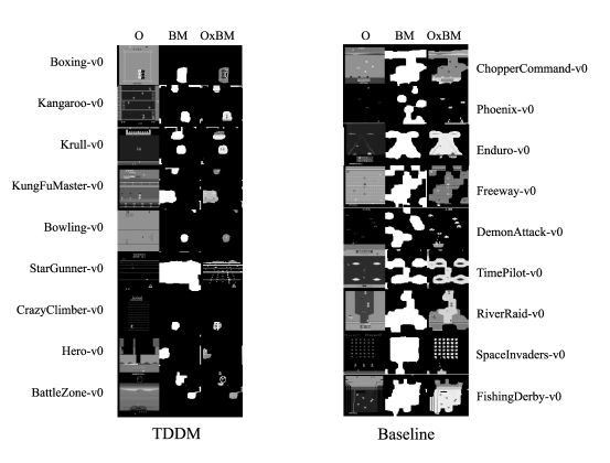
Figure 5: Masking dynamics comparing the best performing benchmarked games under TDDM models (left) and the best performing games under regular baseline models (left). Each game is represented by three frames columns, namely (O - Original unfiltered frame; BM - Binary mask obtained under $\displaystyle TDDM$ process outlined in 1; $\displaystyle OxBM$ Final filtered frame in Figure 1 that is forwarded to the learning algorithm or $\displaystyle TDDM(S)$ created by applying element-wise matrix multiplication of $\displaystyle 0$ with the $\displaystyle BM$.

TDDM models bias towards states with a higher discriminatory potential, as quantified by the amount of masking, may be seen as temporal-information greediness, or indirectly generated artificial attention capability.

This temporal-information-greedy behavior can be also observed, even more clearly, in the informational content of the LSTM states that propagate context-creating temporal information through LSTM’s sequential process as depicted in Figure 4.

In order to quantify the ability of $\displaystyle TDDM$ models to distinguish between the static and temporally correlated information, and then focus on the latter, it is possible to examine the actual level of utilization of the LSTM recurrent layer during the realization of the agent’s policy. The LSTM utilization is represented by the amount of informational entropy contained in the layer’s hidden states, which, in case of LSTM architectures, are the main propagators of contextual, temporally related information. The experimental measures reported in section $\displaystyle b)$ of Figure 6 indicate that, regardless of the presented environment/game, the $\displaystyle TDDM$ learned models displayed levels of their $\displaystyle LSTM$ layer hidden states entropy significantly higher than their baseline counterparts. This trend is visible in the upper right corner of the plot showing a high distribution density of the $\displaystyle TDDM$ category.

As this type of information is more crucial in forming the agent’s belief state, the agents that exhibit bias towards it can be seen as more effective in their utilization of the communication channel between their own perception and the learning algorithm. The agents that used $\displaystyle TDDM$ models in identical and reproducible benchmark trials, according to Figure 6 $\displaystyle b)$ propagated higher levels of temporally correlated information from the environment to the learning algorithm.

The ability of (artificial or biological) agent to convey a specific type of information that is more descriptive of the environment dynamics, or perturbations, increases its ability to produce more credible belief states. As we can see from Figure 6 $\displaystyle(b)$ acting optimally in a dynamic environment benefits from belief state representations that indeed contain in themselves necessary temporal abstractions crucial to organism survival and, in the case of an artificial agent, to its ability to maximize the expected return of a reinforcement function in the long run.

While the a) and b) plots of Figure 6 are mostly descriptive of the difference in information processing dynamics, the second row (plots c) and d)) puts in evidence the difference in exploration/exploitation dispositions of the agents using models trained with $\displaystyle TDDM$ approach with respect to the baseline ones. From Figure 6 c) it is evident that the $\displaystyle TDDM$ models have produced policies that in general allow for longer Atari game episodes, which, in most of the game variations, accounts for a higher exploration rate of the game state space.

On the contrary, Figure 6 d) indicates that rewards for the $\displaystyle TDDM$ models are more consistent, as quantified by their variance. While plot 6 c) seems to suggest a more efficient exploration of the game state space, the d) plot also accounts for the $\displaystyle TDDM$ models ability to exploit the reliability of Q-value predictions in such a way as to be able to predict the return more consistently than their baseline counterparts.

Environment	A.R	N.P.E	H.S.A.E	S.A.E	H.S.S	M.A	S.S	ST.D.R	ST.D.A	ST.D.M
Alien-v0	0.7064	747	5.094	8.56	1.166	70.42	214.1	4.073	6.094	700.5
Alien-v0	0.7889	670.5	6.664	8.531	2.423	70.03	217	8.127	4.734	656.7
Asterix-v0	0.6217	1280	4.981	8.437	1.769	74.09	382.3	5.56	1.388	1095
Asterix-v0	0.7964	1366	7.35	8.333	2.657	82.03	315.5	6.286	1.997	1031
Asteroids-v0	1.436	1165	8.61	8.61	10.24	96.78	512	9.586	3.753	191.1
Asteroids-v0	1.349	792.9	8.61	8.61	10.24	96.79	512	9.641	3.573	208.8
Atlantis-v0	9.158	649.1	6.652	8.472	2.71	78.61	359.7	111.6	1.197	694
Atlantis-v0	9.805	675.5	8.48	8.582	6.105	77.78	416.6	124.7	1.293	699.7
BattleZone-v0	0.664	2561	8.61	8.61	10.24	84.22	512	32.67	3.785	1115
BattleZone-v0	2.293	566.7	8.61	8.61	10.24	52.74	512	81.9	1.181	752.4
BeamRider-v0	0.05842	8.176e+04	8.61	8.61	10.24	92.4	512	1.627	0.9999	1220
BeamRider-v0	0.737	215.2	8.608	8.599	10.02	13.14	510	5.744	2.062	1100
Berzerk-v0	1.063	2066	8.6	8.6	10.05	73.34	510.7	7.256	4.509	959.8
Berzerk-v0	0.9837	1958	8.599	8.566	8.988	73.74	500	6.973	4.366	947
Bowling-v0	0.000845	10	8.61	8.61	10.24	98.1	512	0.07489	0.8484	180.3
Bowling-v0	0.002796	18.6	8.61	8.61	10.24	98.99	512	0.09414	0.8768	121.5
Boxing-v0	-0.008385	57.9	5.35	6.723	1.394	89.67	125.1	0.3677	3.736	450.4
Boxing-v0	0.004923	65.9	7.714	8.616	6.63	91.44	388.2	0.3479	3.999	471.4
Breakout-v0	0.00021	8.958e+04	8.61	8.61	10.24	48.97	512	0.01679	0.9616	1501
Breakout-v0	0.02164	1225	8.61	8.61	10.24	92.97	512	0.1991	0.9374	326
ChopperCommand-v0	1.675	526.6	8.602	8.598	9.271	60.17	510.7	14.9	5.761	713.9
ChopperCommand-v0	1.39	459.4	8.591	8.594	4.14	56.91	427.6	14.64	2.521	623.4
CrazyClimber-v0	0.1476	283.2	8.571	8.608	10.18	84.66	511.9	3.839	0.6595	538.5
CrazyClimber-v0	1.103	157	8.612	8.567	6.56	89.08	482.6	10.45	1.763	784.3
DemonAttack-v0	0.2449	819.1	8.61	8.61	10.1	87.64	512	1.702	1.519	763.3
DemonAttack-v0	0.004	5.231e+04	8.61	8.61	10.23	92.12	512	0.2015	1.646	428.3
Enduro-v0	0.02173	30	8.125	8.61	6.046	70.53	467.1	0.2403	2.655	1148
Enduro-v0	0.001997	30	8.116	8.612	9.018	66.62	482.7	0.1799	2.625	1082
FishingDerby-v0	-0.02089	52.8	8.61	8.61	10.24	40.48	512	0.277	5.345	315.3
FishingDerby-v0	-0.03175	53.6	8.61	8.61	10.24	38.22	512	0.2686	5.455	334.7
Freeway-v0	0	50.1	8.61	8.61	10.24	39.99	512	0	0.1281	664.8
Freeway-v0	0.009295	50	8.61	8.61	10.24	37.37	512	0.09596	0.5826	663.2
Frostbite-v0	0.2432	4452	5.831	8.475	1.842	57.26	227.6	1.54	5.08	1897
Frostbite-v0	0.2599	1249	6.526	8.482	3.041	59.3	270.7	1.591	4.58	1817
Hero-v0	0.02497	343.9	8.492	8.521	3.952	91.08	388.9	2.697	3.828	724.5
Hero-v0	0.1651	473.4	5.267	8.568	3.383	90.76	313.9	8.428	5.199	682.4
IceHockey-v0	-0.0048	28.6	8.61	8.61	10.24	87.59	512	0.07606	3.889	277.8
IceHockey-v0	-0.002695	27	8.61	8.61	10.24	88.08	512	0.08236	3.934	308.5
Jamesbond-v0	0.2138	932.4	8.61	8.61	10.24	60.55	512	3.263	5.016	1098
Jamesbond-v0	0.2576	1188	8.603	8.601	10.14	59.98	511.6	3.58	4.882	1110
Kangaroo-v0	0.4452	865.4	8.603	8.603	10.1	83.45	511.4	9.43	4.22	768.8
Kangaroo-v0	0.9237	827.7	8.586	8.578	10.1	83.73	510.6	13.56	3.765	757.4
Krull-v0	0.2896	161.9	8.516	8.576	5.926	68.56	425.3	1.901	4.28	2001
Krull-v0	0.6939	176.1	8.146	8.61	7.116	61.28	432.6	2.919	5.47	2299
KungFuMaster-v0	0.0282	987	8.61	8.61	10.24	95.64	512	2.375	3.216	401.1
KungFuMaster-v0	0.7838	698.4	8.567	8.532	3.271	87.42	376.8	12	4.123	687.7
Phoenix-v0	0.6441	1255	3.841	8.63	0.7936	83.61	223.3	7.617	2.068	636
Phoenix-v0	0.133	1496	6.025	8.632	1.855	86.67	366.4	2.776	0.6282	487.4
Pitfall-v0	-0.05164	1273	8.61	8.61	10.24	82.39	512	0.4363	1.865	876.9
Pitfall-v0	-0.05085	1.332e+04	8.61	8.61	10.24	80.52	512	0.4312	5.258	710.4
Pong-v0	-0.004044	35.4	8.61	8.61	10.24	91.32	512	0.1014	1.803	429.7
Pong-v0	-0.01118	68.5	8.61	8.61	10.24	89.4	512	0.1271	1.524	412.1
Qbert-v0	1.367	1615	6.482	8.478	2.579	84.69	294.8	12.98	1.729	300.2
Qbert-v0	1.599	1964	6.477	8.469	2.922	83.97	284.2	13.77	1.494	305.9
Riverraid-v0	3.015	880.9	7.577	8.451	3.429	74.52	323	22.01	6.135	1302
Riverraid-v0	2.349	1613	6.701	8.323	2.776	74.42	329.6	13.38	5.081	1261
Seaquest-v0	0.3839	627	8.61	8.61	10.21	75.03	511.9	2.764	4.838	748.6
Seaquest-v0	0.3393	682.9	8.588	8.577	9.127	73.99	506.7	2.604	4.687	720.5
SpaceInvaders-v0	0.4755	761.7	8.499	8.607	8.431	82.9	504.5	3.874	1.593	1017
SpaceInvaders-v0	0.3813	918	8.506	8.598	7.273	82.1	493.2	3.576	1.561	1073
StarGunner-v0	0.0472	484.3	8.61	8.61	10.24	71.69	512	2.901	1.535	743.2
StarGunner-v0	0.7814	721.6	8.61	8.61	10.24	72.44	512	12.47	2.567	699.2
TimePilot-v0	2.172	815.5	8.61	8.61	10.22	75.96	511.8	58.96	2.132	1329
TimePilot-v0	1.132	779.3	8.674	8.637	2.69	70.23	338.4	34.64	1.27	1344
#TDDM	20	18	13	13	16	19	16	20	15	12
#benchmark	12	15	19	19	20	13	22	12	17	20

Table 1: Results of the Evaluation Benchmark performed under identical reproducible setups. Best performing batches are outlined in bold for each of the game environments and results obtained with models trained under $\displaystyle TDDM$ are highlighted with light-gray background; The last two rows represent a summary of best performing values for each of the columns: #TDDM row represents the number of best values among the batches obtained by using models trained under $\displaystyle TDDM$ while the #Benchmark row does the same with the baseline models. Detailed description of the specific columns used are presented in Table 2.

Abbreviation	Full Name	Description
Environment	Environment	Specific Atari game used in benchmark batch.
A.R.	Average Return	The immediate rewards that the agents received averaged over all of the 10 trials that formed a single benchmark batch.
N.P.E.	Number of Played Episodes	Average Total Number of Played Episodes in a single trial.
H.S.A.E.	Hidden States Activation Entropy	Average Shannon’s entropy in bits of the model’s hidden states $\displaystyle H_{n}$ indicative of the amount of information being effectively propagated through their activations in the LSTM part of the main ANN model detailed in 4.
S.A.E.	States Activation Entropy	Average Shannon’s entropy in bits of the model’s input states $\displaystyle X_{n}$ indicative of the amount of information being effectively propagated through their activations in the LSTM part of the main ANN model detailed in 4.
H.S.S.	Hidden States Sparsity	Average Percentage of Non-Zero Hidden States Activations. Higher percentage indicates more activity in RNN Hidden States propagation.
M.A.	Masking Amount	Percentage of the input state’s pixels masked or blanked with $\displaystyle TDDM$.
S.S.	States Sparsity	Percentage of Non-Zero model’s input states $\displaystyle X_{n}$ Activations. Higher percentage indicates more activity in RNN input state propagation.
ST.D.R	Standard-Deviation of Returns	Depending on a specific environment reinforcement function the variance of the Returns could be an indicative of an agent’s preference of exploration over exploitation.
ST.D.A	Standard-Deviation of Selected Actions	Depending on a specific environment configuration the variance of the Actions taken could be an indicative of an agent’s preference of exploration over exploitation.
ST.D.M	Standard-Deviation of Masking Percentages	The variance in Masking Amounts of single frames could indicate the level of adaptability of the motion detection technique shown in Figure 1 to a specific environment.

Table 2: Detailed Description of the type of data represented in the columns of Table 6.

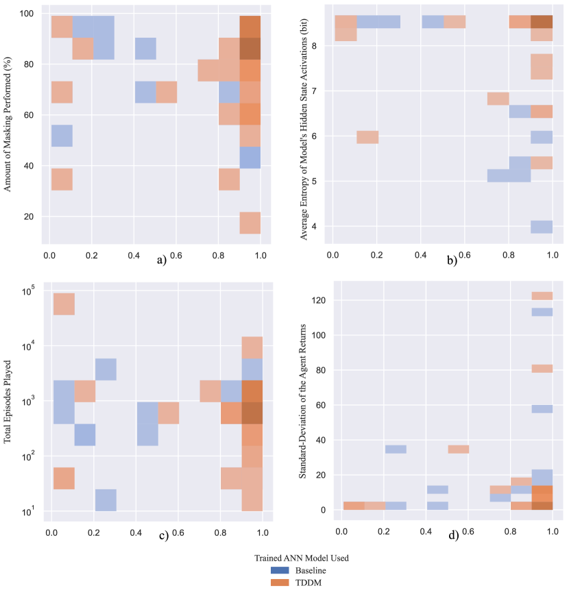
Figure 6: Visualization of distribution densities for four characterizing variables (ordinates) selected from Table 6 across the relative agent’s returns normalized in the range $\displaystyle(0-1)$ (abscissa). The plotted areas represent counts of ordinate-variable observations falling within each discrete bin; higher frequencies correspond to higher saturation values. Areas hues are indicative of the trained model used in the evaluation trial: benchmark results obtained using models trained under $\displaystyle TDDM$ approach have their frequencies or counts represented in magenta while the benchmark results obtained using baseline models are indicated in blue.

7 Concluding Remarks

The abundance of the inherent information-generating uncertainty in our perception of the world pushed the human evolution into a momentum of producing information-processing mechanisms with increasing complexity that would in turn be able to reduce this uncertainty on a variety of levels or abstraction including crafting our immediate environment by creating patterns of predictability; be it in a form of ubiquitous technical systems (which include the artificial learning ones presented in this work) or the more abstract social structures.

Interaction and causal relationships with the perceived environment are emerging as the focus of the perception-based information-gathering process rather than expanding the perception domain itself. For example, an agent would not benefit from a hypothetical super-perception that would enable it to perceive the amount of information contained in the spin direction of electrons in each of the atoms of a typical physical object; if a state of spin can be either spin-up or spin-down with equal probability distribution, this would give us an entropy of 1 bit per electron. This information though, will not support the determination of the interaction that physical objects have with their surroundings or provide a learning mechanism with the representation of perturbations of the environment significant to its survival, e.g., temperature, sound, vision.

Interacting with a more predictable environment reduces the overall information that needs to be processed, but at the same time generates more information that explains the causal relationships within. This causal subset of the perceived information can be seen as an information gain of interaction (or transition from $\displaystyle s$ to $\displaystyle s^{\prime}$ in our case) that is irreducible to its composing parts ($\displaystyle s$ and $\displaystyle s^{\prime}$) according to the integrated information principle or $\displaystyle\Phi$ proposed by [59].

Depending on the specific machine learning approach, an artificial learning agent capable of discriminating the perceived information based on a temporal or a spatial context can be more effective to convert that same information into higher order representations, such as Q-values that would eventually lead to the creation of better policies.

The main insight obtained from this work is that perceptual discrimination based on temporal difference displacement, or $\displaystyle TDD$ criterion, as evident from Table 6, may enable convergence of temporal-difference learning algorithms to their optimal policies in fewer learning steps ; moreover, it can produce learned models that perform better than a state-of-art baseline in 20 out of 32 different Atari games, under the identical and reproducible setups.

It can be also noted that the models learned under $\displaystyle TDD$ masking possess a strong tendency towards an increased utilization of the recurrent LSTM section of the main Q-approximator shown in Figure 3, effectively utilizing more of the temporally correlated information ([59]) in the creation of the agent’s belief state leading to overall better agent’s performances in the benchmark, as indicated in Table 6.

8 Acknowledgments

This article has been supported by the OP RDE funded project Research Center for Informatics No.: CZ.02.1.01/0.0./0.0./16_019/0000765.

Appendix A.

In this appendix we present the variation of a total of three variables characterizing the actual learning during the agent’s training phase, namely: total cumulative return, average Q-value, and number of played episodes.

Table 3: Total cumulative return received during the training phase for each of the combinations of environment/masking. Best values are highlighted in bold.

Table 4: Average Q-value reached during the training phase for each of the combinations of environment/masking. Best values are highlighted in bold.

Table 5: Average number of episodes played during the training phase for each of the combinations of environment/masking. Best values are highlighted in bold. Higher values are indicative of a exploratory strategy.

References

- Abadi et al. [2016] Abadi, M., Barham, P., Chen, J., Chen, Z., Davis, A., Dean, J., Devin, M., Ghemawat, S., Irving, G., Isard, M., et al., 2016. Tensorflow: A system for large-scale machine learning, in: 12th USENIX Symposium on Operating Systems Design and Implementation (OSDI 16), pp. 265–283.
- Agre [1988] Agre, P.E., 1988. The dynamic structure of everyday life. Technical Report. Massachusetts Inst Of Tech Cambridge Artificial Intelligence Lab.
- Agre and Chapman [1987] Agre, P.E., Chapman, D., 1987. Pengi: An implementation of a theory of activity., in: AAAI, pp. 286–272.
- Araya et al. [2010] Araya, M., Buffet, O., Thomas, V., Charpillet, F., 2010. A pomdp extension with belief-dependent rewards, in: Advances in neural information processing systems, pp. 64–72.
- Ashby [1961] Ashby, W.R., 1961. An introduction to cybernetics. Chapman & Hall Ltd.
- Åström [1965] Åström, K.J., 1965. Optimal control of markov processes with incomplete state information. Journal of Mathematical Analysis and Applications 10, 174–205.
- Baddeley [1992] Baddeley, A., 1992. Working memory. Science 255, 556–559.
- Ballard et al. [1997] Ballard, D.H., Hayhoe, M.M., Pook, P.K., Rao, R.P., 1997. Deictic codes for the embodiment of cognition. Behavioral and brain sciences 20, 723–742.
- Bellman [1966] Bellman, R., 1966. Dynamic programming. Science 153, 34–37.
- Boisseau et al. [2016] Boisseau, R.P., Vogel, D., Dussutour, A., 2016. Habituation in non-neural organisms: evidence from slime moulds. Proceedings of the Royal Society B: Biological Sciences 283, 20160446.
- Boutilier [2002] Boutilier, C., 2002. A pomdp formulation of preference elicitation problems, in: AAAI/IAAI, pp. 239–246.
- Broadbent [1958] Broadbent, D., 1958. E.(1958). Perception and communication .
- Brockman et al. [2016] Brockman, G., Cheung, V., Pettersson, L., Schneider, J., Schulman, J., Tang, J., Zaremba, W., 2016. Openai gym. arXiv:arXiv:1606.01540.
- Campbell [1974] Campbell, D.T., 1974. Evolutionary epistemology. volume 1. na.
- Cassandra et al. [1994] Cassandra, A.R., Kaelbling, L.P., Littman, M.L., 1994. Acting optimally in partially observable stochastic domains, in: AAAI, pp. 1023–1028.
- de Castro et al. [2019] de Castro, M.S., Congeduti, E., Starre, R., Czechowski, A., Olihoek, F., 2019. Influence-aware memory for deep reinforcement learning. arXiv preprint arXiv:1911.07643 .
- Chapman [1992] Chapman, D., 1992. Intermediate vision: Architecture, implementation, and use. Cognitive Science 16, 491–537.
- Chrisman [1992] Chrisman, L., 1992. Reinforcement learning with perceptual aliasing: The perceptual distinctions approach, in: AAAI, Citeseer. pp. 183–188.
- Chrisman et al. [1991] Chrisman, L., Caruana, R., Carriker, W., 1991. Intelligent agent design issues: Internal agent state and incomplete perception, in: Proceedings of the AAAI Fall Symposium on Sensory Aspects of Robotic Intelligence. AAAI Press/MIT Press, Citeseer.
- Conant and Ross Ashby [1970] Conant, R.C., Ross Ashby, W., 1970. Every good regulator of a system must be a model of that system. International journal of systems science 1, 89–97.
- Csikszentmihalyi [1992] Csikszentmihalyi, M., 1992. Imagining the self: An evolutionary excursion. Poetics 21, 153–167.
- Farnebäck [2003] Farnebäck, G., 2003. Two-frame motion estimation based on polynomial expansion, in: Scandinavian conference on Image analysis, Springer. pp. 363–370.
- Friston [2010] Friston, K., 2010. The free-energy principle: a unified brain theory? Nature reviews neuroscience 11, 127–138.
- Hausknecht and Stone [2015] Hausknecht, M., Stone, P., 2015. Deep recurrent q-learning for partially observable mdps, in: 2015 AAAI Fall Symposium Series.
- Hayhoe et al. [1997] Hayhoe, M., Bensinger, D., Ballard, D., 1997. Task constraints in visual working memory .
- Hochreiter and Schmidhuber [1997] Hochreiter, S., Schmidhuber, J., 1997. Long short-term memory. Neural computation 9, 1735–1780.
- Jordan and Rumelhart [1992] Jordan, M.I., Rumelhart, D.E., 1992. Forward models: Supervised learning with a distal teacher. Cognitive science 16, 307–354.
- Kirchner and Srinivasan [1989] Kirchner, W., Srinivasan, M., 1989. Freely flying honeybees use image motion to estimate object distance. Naturwissenschaften 76, 281–282.
- Le et al. [2018] Le, T.P., Vien, N.A., Chung, T., 2018. A deep hierarchical reinforcement learning algorithm in partially observable markov decision processes. Ieee Access 6, 49089–49102.
- Lee et al. [2008] Lee, W.S., Rong, N., Hsu, D., 2008. What makes some pomdp problems easy to approximate?, in: Advances in neural information processing systems, pp. 689–696.
- Lin [1991] Lin, L.J., 1991. Programming robots using reinforcement learning and teaching, in: Proceedings of the ninth National conference on Artificial intelligence-Volume 2, pp. 781–786.
- Lovejoy [1991] Lovejoy, W.S., 1991. A survey of algorithmic methods for partially observed markov decision processes. Annals of Operations Research 28, 47–65.
- Marr [1976] Marr, D., 1976. Early processing of visual information. Philosophical Transactions of the Royal Society of London. B, Biological Sciences 275, 483–519.
- Marr [1982] Marr, D., 1982. Vision: A computational investigation into the human representation and processing of visual information, henry holt and co. Inc., New York, NY 2.
- McCallum [1993] McCallum, R.A., 1993. Overcoming incomplete perception with utile distinction memory, in: Proceedings of the Tenth International Conference on Machine Learning, pp. 190–196.
- Mnih et al. [2013] Mnih, V., Kavukcuoglu, K., Silver, D., Graves, A., Antonoglou, I., Wierstra, D., Riedmiller, M., 2013. Playing atari with deep reinforcement learning. arXiv preprint arXiv:1312.5602 .
- Mnih et al. [2015] Mnih, V., Kavukcuoglu, K., Silver, D., Rusu, A.A., Veness, J., Bellemare, M.G., Graves, A., Riedmiller, M., Fidjeland, A.K., Ostrovski, G., et al., 2015. Human-level control through deep reinforcement learning. Nature 518, 529–533.
- Monahan [1982] Monahan, G.E., 1982. State of the art—a survey of partially observable markov decision processes: theory, models, and algorithms. Management science 28, 1–16.
- Nilsson [1996] Nilsson, D.E., 1996. Eye ancestry: old genes for new eyes. Current Biology 6, 39–42.
- Ong et al. [2009] Ong, S.C., Png, S.W., Hsu, D., Lee, W.S., 2009. Pomdps for robotic tasks with mixed observability., in: Robotics: Science and systems, p. 4.
- Rabiner and Juang [1986] Rabiner, L., Juang, B., 1986. An introduction to hidden markov models. ieee assp magazine 3, 4–16.
- Ramicic and Bonarini [2017] Ramicic, M., Bonarini, A., 2017. Entropy-based prioritized sampling in deep q-learning, in: 2017 2nd International Conference on Image, Vision and Computing (ICIVC), IEEE. pp. 1068–1072.
- Rampino and Caldeira [1994] Rampino, M.R., Caldeira, K., 1994. The goldilocks problem: climatic evolution and long-term habitability of terrestrial planets. Annual Review of Astronomy and Astrophysics 32, 83–114.
- Rankin [2004] Rankin, C.H., 2004. Invertebrate learning: what can’t a worm learn? Current biology 14, R617–R618.
- Rosner and Homberg [2013] Rosner, R., Homberg, U., 2013. Widespread sensitivity to looming stimuli and small moving objects in the central complex of an insect brain. Journal of Neuroscience 33, 8122–8133.
- Ross et al. [2008] Ross, S., Pineau, J., Paquet, S., Chaib-Draa, B., 2008. Online planning algorithms for pomdps. Journal of Artificial Intelligence Research 32, 663–704.
- Salway and Logie [1995] Salway, A.F., Logie, R.H., 1995. Visuospatial working memory, movement control and executive demands. British Journal of Psychology 86, 253–269.
- Schrittwieser et al. [2020] Schrittwieser, J., Antonoglou, I., Hubert, T., Simonyan, K., Sifre, L., Schmitt, S., Guez, A., Lockhart, E., Hassabis, D., Graepel, T., et al., 2020. Mastering atari, go, chess and shogi by planning with a learned model. Nature 588, 604–609.
- Shannon [1948] Shannon, C.E., 1948. A mathematical theory of communication. The Bell system technical journal 27, 379–423.
- Silver et al. [2018] Silver, D., Hubert, T., Schrittwieser, J., Antonoglou, I., Lai, M., Guez, A., Lanctot, M., Sifre, L., Kumaran, D., Graepel, T., et al., 2018. A general reinforcement learning algorithm that masters chess, shogi, and go through self-play. Science 362, 1140–1144.
- Silver et al. [2017] Silver, D., Schrittwieser, J., Simonyan, K., Antonoglou, I., Huang, A., Guez, A., Hubert, T., Baker, L., Lai, M., Bolton, A., et al., 2017. Mastering the game of go without human knowledge. Nature 550, 354–359.
- Simmons et al. [2010] Simmons, P.J., Rind, F.C., Santer, R.D., 2010. Escapes with and without preparation: the neuroethology of visual startle in locusts. Journal of insect physiology 56, 876–883.
- Spaan [2008] Spaan, M.T., 2008. Cooperative active perception using pomdps, in: AAAI 2008 workshop on advancements in POMDP solvers.
- Spaan et al. [2015] Spaan, M.T., Veiga, T.S., Lima, P.U., 2015. Decision-theoretic planning under uncertainty with information rewards for active cooperative perception. Autonomous Agents and Multi-Agent Systems 29, 1157–1185.
- Srinivasan [2020] Srinivasan, M.V., 2020. Vision, perception, navigation and ‘cognition’in honeybees and applications to aerial robotics. Biochemical and Biophysical Research Communications .
- Sutton [1991] Sutton, R.S., 1991. Dyna, an integrated architecture for learning, planning, and reacting. ACM Sigart Bulletin 2, 160–163.
- Sutton and Barto [2018] Sutton, R.S., Barto, A.G., 2018. Reinforcement learning: An introduction. MIT press.
- Tang et al. [2020] Tang, Y., Nguyen, D., Ha, D., 2020. Neuroevolution of self-interpretable agents, in: Proceedings of the 2020 Genetic and Evolutionary Computation Conference, pp. 414–424.
- Tononi et al. [2016] Tononi, G., Boly, M., Massimini, M., Koch, C., 2016. Integrated information theory: from consciousness to its physical substrate. Nature Reviews Neuroscience 17, 450–461.
- Tsitsiklis [1994] Tsitsiklis, J.N., 1994. Asynchronous stochastic approximation and q-learning. Machine learning 16, 185–202.
- Ullman [1987] Ullman, S., 1987. Visual routines, in: Readings in computer vision. Elsevier, pp. 298–328.
- Vinyals et al. [2019a] Vinyals, O., Babuschkin, I., Chung, J., Mathieu, M., Jaderberg, M., Czarnecki, W.M., Dudzik, A., Huang, A., Georgiev, P., Powell, R., et al., 2019a. Alphastar: Mastering the real-time strategy game starcraft ii. DeepMind blog , 2.
- Vinyals et al. [2019b] Vinyals, O., Babuschkin, I., Czarnecki, W.M., Mathieu, M., Dudzik, A., Chung, J., Choi, D.H., Powell, R., Ewalds, T., Georgiev, P., et al., 2019b. Grandmaster level in starcraft ii using multi-agent reinforcement learning. Nature 575, 350–354.
- Watkins and Dayan [1992] Watkins, C.J., Dayan, P., 1992. Q-learning. Machine learning 8, 279–292.
- Weyns et al. [2004] Weyns, D., Steegmans, E., Holvoet, T., 2004. Towards active perception in situated multi-agent systems. Applied Artificial Intelligence 18, 867–883.
- Whitehead and Ballard [1990] Whitehead, S.D., Ballard, D.H., 1990. Active perception and reinforcement learning, in: Machine Learning Proceedings 1990. Elsevier, pp. 179–188.
- Whitehead and Ballard [1991] Whitehead, S.D., Ballard, D.H., 1991. Learning to perceive and act by trial and error. Machine Learning 7, 45–83.
- Wierstra and Wiering [2004] Wierstra, D., Wiering, M., 2004. Utile distinction hidden markov models, in: Proceedings of the twenty-first international conference on Machine learning, p. 108.
- Zhu et al. [2017] Zhu, P., Li, X., Poupart, P., Miao, G., 2017. On improving deep reinforcement learning for pomdps. arXiv preprint arXiv:1704.07978 .