Boson peak in amorphous systems: role of phonon mediated coupling of nano-clusters

Abstract

Based on a description of an amorphous solid as a collection of coupled nanosize molecular clusters referred as basic blocks, we analyse the statistical properties of its Hamiltonian. The information is then used to derive the ensemble averaged density of the vibrational states (non-phonon) which turns out to be a Gaussian in the bulk of the spectrum and an Airy function in the low frequency regime. A comparison with experimental data for five glasses confirms validity of our theoretical predictions.

I Introduction

.

As indicated by many experiments on disordered materials, the vibrational density of states (VDOS) in the energy range $(2\to 10)\times 10^{-22}\;J$ exceeds significantly beyond that of the phonon contribution. Referred as the boson peak, the functional form of the excess VDOS is found to be universal for a wide range of amorphous systems irrespective of their microscopic details (i.e with different chemical bonding and short-range order structure, specifically for the close packed metals and the covalent networks) buch2 ; vdos . The primary objective of this study is to seek this functional form using standard statistical tools.

Previous attempts to understand the physical origin of the boson peak and other glass anomalies are usually based on various phenomenological models of the local interactions dpr ; ell3 e.g. whether the underlying structural disorder is of harmonic or anharmonic type. In the models based on harmonic degrees of freedom e.g. coupled harmonic oscillators with randomized force constants, the excess VDOS marks the transition between acoustic like excitations and a vibrational spectrum dominated by disorder sdg ; tara ; grig . On the contrary, the soft potential model (SPM) suggests the vibrations of atoms in the strongly anharmonic potentials (the non-acoustic quasi local vibrations or QLV) as the cause spm ; gure ; psg . Based on numerical simulations, the heterogeneous elasticity theory suggest the boson peak to originate from the spatial fluctuations of the elastic constants on a microscopic length scale schi2 . A first order transition theory relates the BP to the dynamics of domain walls that separate cooperatively rearranging regions lw . Another theory predicts the characteristic vibrations of nanometric clusters as the cause of boson peak; the vibrations are believed to exist e.g due to spatially inhomogeneous cohesion in glasses du ; mns ; sksq . Analytical attempts to derive VDOS, based on a random matrix modelling of the dynamical (or Hessian) matrix of an amorphous solid, have also been considered e.g. grig ; ml ; smmm ; bp ; zac ; for example, the harmonic random matrix models (HRM) of Hamiltonian or dynamical matrix suggest the boson peak to originate from purely harmonic elastic disorder sdg ; schi2 ; grig ; srs ; gual ; zac . The excess VDOS is also suggested as the disorder induced modified form of Van Hove singularities of the crystal chum . Research during last two decades has introduced some new approaches too e.g. models based on effective medium theories wyt ; degi of marginal elastic instability near a characteristic frequency or on randomly jammed particles at zero temeperature interacting through pairwise potentialsosln ; mizu .

Although leading to many important physical insights in the low temperature anomalies, a weak aspect of almost all these models is a lack of unanimity and their dependence on widely different assumptions of the underlying interactions and nature of disorder. The need to establish the veracity of these assumptions motivated large scale numerical simulations which not only indicated failure of many quantitative predictions of these models but fail to reach to a consensus too. For example, for very low frequencies $\omega<\omega_{0}$, recent SPM models theoretically predict the VDOS behavior as $\rho(\omega)\propto{\omega^{4}\over\omega_{bp}^{3}}$ gure ; psg ; here $\omega_{0}$ is a characteristic frequency of the solid. While agreeing with qualitative prediction of the SPM model, the numerical study mizu , based on the model of pairwise interacting randomly jammed particles, reports quantitative differences. On the contrary, the effective medium theories (EMT) based on marginal instability near boson peak differ from both SPM model as well as mizu and predict the low frequency VDOS behavior as $\rho(\omega)\propto{\omega^{2}\over(\omega^{*})^{2}}$ (for $\omega<\omega_{0}$), significantly bigger than the Debye prediction $\rho(\omega)={\omega^{2}\over(\omega^{*})^{3/2}}$ wyt ; degi with $\omega^{*}$ as another characteristics frequency of the material. A similar non-Debye scaling of VDOS is also reported by the replica theory approach fpuz . Although the experimental study lern indicates $\omega^{4}$ dependnece of VDOS at low $\omega$, it does not rule it out as an artefact of the cooling process. The numerical study in rpcv claims a disagreement of most of the observations with results based on HRM models srs ; gual but agreement with QLV model spm without using adjustable parmeters.

The discord continues in high frequency regime too. EMT assuming marginal stability indicate a characteristic pleateau of VDOS at $\omega>\omega^{*}$ wy1 ; wy2 ; degi A similar behavior is also indicated by the numerical analysis of a jammed particle model mizu although its result in low frequency regime is inconsistent with wyt ; degi . The existence of such a pleateau however is not reported in experimental analysis of amorphous materials e.g. ya26 ; ya27 ; ya21 ; ya28 ; yanno ; hsgms or in Euclidean random matrix approach of grig ; the latter study indeed suggest a semicircle form of VDOS with convex tails. The experimental study of doped crystals indicates a Gaussian form of boson peak hsgms

The exact role of the disorder in various anamolies also adds to further confusion. Although relevant for transport properties, strong experimental evidence indicates its relative insignificance in controlling the Boson peak anamoly. Furthermore, even if justified for some systems, the applicability of the assumptions to wide range of amorphous solids and disordered lattices, where boson peak in observed, is not directly obvious or experimentally observed. Based on experimental evidence, it is expected that for solids with same local structure, irrespective of their long range order i.e crystalline or non-crystaline order, should have similar boson peak amplitude. Besides, it is not sufficient only to know why a particular feature appears in amorphous solids but also why it is absent in crystals. This motivates us to attempt in the present work a theoretical route based on the interactions, experimentally established to be omnipresent at microscopic level and not hypothetical, of the smallest constituents of a generic solid i.e atoms and molecules and seek at to how the reorganization of the local units leads to emergence of collective interactions leading to different physical behavior in amorphous solids.

An inherent suggestion lurking behind many of the experimental observations is that the peak originates from the fundamental interactions which occur in the energy range corresponding to vibrational molecular spectrum and thus give rise to additional density of states (besides the phonon contribution) bb1 ; bb2 ; bb3 . The promising candidate in this context are the molecular interactions at medium range order (MRO) of glasses and their phonon induced coupling at larger length scales vdos ; du ; ell3 ; degi ; sksq ; mg ; bb1 ; bb2 ; bb3 . As revealed by many studies in past, the interactions among the molecules separated by distances less then medium range order are dominated by the Vanderwaal forces isra ; ajs . At larger distances however a collective interaction of the cluster of molecules can lead to emergence of new, modified form of forces bb3 ; arg ; meek ; lhe . A conspiracy between the two types, acting at short and large length scales, can give rise to an arrangement of molecules as a collection of sub-structures e.g spherical clusters in an amorphous solid of macroscopic size. The idea was introduced in a recent theory, describing an amorphous solid of macroscopic size as a collection of nano-size sub-units bb1 ; bb3 ; bb3 . The latter, referred as basic blocks, are subjected to a phonon mediated coupling with each other through their stress fields (arising due to external perturbations); the coupling has an inverse cube dependence on the distance between the block centers vl ; dl ; lg1 . The interactions among molecules within a single block are however dominated by Vanderwaal forces of $1/r^{6}$ type (with $r$ as the distance between the molecules).

Based on the basic block approach, the properties of a macroscopic amorphous solid can be described in terms of those of the basic blocks; for example, the approach was used in bb2 to explain the universality of the internal friction at low temperature. As discussed in bb1 ; bb2 ; bb3 , the properties of a basic block can be derived from the molecular properties which are independent of system-specifics and thereby lead to universalitiy in the low temperature properties e.g specific heat, internal friction, coupling-strength ratio bb1 ; bb3 ; bb3 . The success of our approach at low temperature and nano length scales, renders it relevant to question whether it is applicable at high $T$ too or would it fail similar to TLS models? This is imperative therefore to analyze the viability of the theory to decipher the boson peak orign and is the focus of present work.

As discussed in bb3 , a basic block is small in size (of the order of few inter-molecular distances) and contains approximately $8$ molecules, independent of the system-specifics. Although in bb3 , the shape of the block was assumed spherical, it can be generalized to other shapes without any qualitative effect on its physics. With a small number of molecules distributed within a radius of $\sim 2\;nm$, the pairwise interaction strength bewteen them can be asumed to be almost equal for all pairs; (the assumption is further supported by the many body aspect of intermolecular interactions). This in turn leads to representation of the block Hamiltonain by a dense (or full) random matrix if the basis is chosen to be the non-interacting basis i.e product basis of the single molecule states. These considerations were used in bb2 to derive the ensemble averaged density of states $\langle\rho_{1}(e)\rangle$ for the basic block; the analysis therein indicated that the level-density $\langle\rho(e)\rangle$ has a universal form of a semi-circle with its peak at $x\approx 1/b$ and the bulk of spectrum lying between $0\leq e\leq 2/b$. The parameter $b$ is determined from the molecular properties and is of the order of $10^{18}\;J^{-1}$ for a wide range of amorphous systems.

Neglecting the phonon mediated coupling among the blocks, the density of the states of the macroscopic solid can be obtained by a convolution of those of the basic blocks. Using the standard central limit theorem, it is technically straightforward to show that a convolution of the semi-circles gives rise to a Gaussian distribution. Although this approach seems to justify the appearance of a peak in the density of states of the macroscopic solid, it is based on the assumption of independent blocks. The inclusion of block-block interaction however invalidates the convolution route and a knowledge of block DOS is no longer sufficient. The DOS of the superblock can however be derived by the standard route i.e by expanding the Green’s function in terms of the trace of the moments of its Hamiltonian. The latter is discussed in detail in vl ; dl ; bb2 ; bb3 and is briefly reviewed in section II. The derivation of its matrix elements, in the non-interacting many body basis of the basic blocks, and their statistical behavior is discussed in detail in section III and IV, respectively. The information is used in section V to derive the average DOS. The next section presents a comparison with experimental results. We conclude in section VII with a summary and discussion of our results.

II Superblock Hamiltonian

We consider a macroscopic sample of an amorphous solid, referred here as the superblock. Following the standard route, the Hamiltonian $H$ of a solid of volume $\Omega$ can in general be written as the sum over intra-molecular interactions as well as inter-molecular ones

$$H=\sum_{k}h_{k}({\bf r}_{k})+{1\over 2}\sum_{k,l}{\mathcal{U}}(|{\bf r}_{k}-{\bf r}_{l}|)$$ (1)

with $h_{k}$ as the Hamiltonian of the $k^{th}$ molecule at position ${\bf r}_{k}$ and ${\mathcal{U}}$ as a pairwise molecular interaction with arbitrary range $r_{0}$.

The superblock Hamiltonian can however be represented by an altrenative form. As discussed in bb3 , the experimentally observed medium range ordering in amorphous systems permits $H$ to be described as a collection of basic blocks too. The inter-molecular interactions can now be divided into two types (i) among molecules within a block, referred as the ”self-interactions” or intra-block ones, and, (ii) from one block to another, referred as the ”other body” type or inter-block type. The Hamiltonain$H$ of the superblock can then be expressed as a sum over basic blocks of volume, say $\Omega_{b}$,

$$H=\sum_{s=1}^{g}{\mathcal{H}}^{(s)}+{1\over 2}\sum_{s,t=1}^{g}\sum_{k\in s,l\in t}{\mathcal{U}}(|{\bf r}_{k}-{\bf r}_{l}|)$$ (2)

where ${\mathcal{H}}^{(s)}$ is the Hamiltonian of a basic block labeled ${}^{\prime\prime}s^{\prime\prime}$, basically sum over the ”self-interactions” i.e molecular interactions within a block. Here $g$ is the total number of blocks, given by $g={\Omega\over\Omega_{b}}$ with $\Omega_{b}$ as the volume of the basic block. As discussed in bb1 ; bb2 ; bb3 and also mentioned in section I, a basic block size is typically of medium range order of the material, with $\Omega_{b}\sim 10^{-20}\;cm^{3}$. Consequently a superblock of typical experimental size $1\;cm^{3}$ consists of $g\approx 10^{20}$ basic blocks.

As discussed in arg ; meek ; lhe ; bb3 , the net molecular force of one block on another can also be described by an effective stress field. Assuming the isotropy and the small block-size, it can be replaced by an average stress field at the center, say ${\bf R_{s}}$, of the block. In presence of an elastic strain field, say $e_{\alpha\beta}$ e.g of the phonons in the material, the stress fields of the blocks interact with phonons strain field and $H$ in eq.(2) can then be expressed as the sum over phonons contribution, say $H_{ph}$, sum over those of non-interacting blocks and the terms describing stress-strain interaction (i.e coupling between phonons and blocks). Let $\Gamma^{(s)}_{\gamma\delta}({\bf r})$ be the stress tensor at point ${\bf R_{s}}$ of the basic block ”s”, $H$ can then be written as

$$H=H_{ph}+\sum_{s=1}^{g}{\mathcal{H}}^{(s)}+\sum_{s=1}^{g}e_{\alpha\beta}\;\Gamma^{(s)}_{\gamma\delta}$$ (3)

Note the last term in the above equation takes into account the molecular-interactions between blocks in eq.(2).

As the strain tensor $e_{\alpha\beta}$ contains a contribution from the phonon field, the exchange of virtual phonons will give rise to an effective (RKKY-type) coupling between the stress tensors of any two block-pairs. The total phonon mediated coupling among all blocks can then be approximated as vl ; dl

$$V=\sum_{s,t;s\not=t}V_{st} = {1\over 8\pi\rho_{m}v_{a}^{2}}\;\sum_{s,t;s\not=t}\;\sum_{\alpha\beta\gamma\delta}\;{\kappa^{(st)}_{\alpha\beta\gamma\delta}\over|\;{\bf R_{s}}-{\bf R_{t}}\;|^{3}}\;\;\Gamma^{(s)}_{\alpha\beta}\otimes\;\Gamma^{(t)}_{\gamma\delta}$$ (4)

with $\sum_{s,t}$ as the sum over all basic blocks, $\rho_{m}$ as the mass-density and $v_{a}$, ($a=l,t$), as the speed of sound in the amorphous material in logitudinal or transverse directions. Here the subscripts $\alpha\beta\gamma\delta$ refer to the tensor components of the stress operator, with notation $\sum_{te}$ implying a sum over all tensor components: $\sum_{te}\equiv\sum_{\alpha\beta\gamma\delta}$. The directional dependence of the interaction is represented by $\kappa^{(st)}_{\alpha\beta\gamma\delta}=\kappa^{(st)}(\theta,\phi)$; it is assumed to depend only on the relative orientation ($\theta,\phi$) of the block-pairs and is independent from their relative separation dl :

$$\kappa^{(st)}_{ijkl} = \nu_{0}\sum_{ijkl}\left(\delta_{jl}\delta_{ik}+\delta_{jk}\delta_{il}\right)+\nu_{2}\;\delta_{ij}\delta_{kl}-3\;\nu_{1}\sum_{ijkl}\left(n_{j}n_{l}\delta_{ik}+n_{j}n_{k}\delta_{il}+n_{i}n_{k}\delta_{jl}+n_{i}n_{l}\delta_{jk}\right)$$ (5)

$$- 3\;\nu_{2}\;\sum_{ijkl}\left(n_{i}n_{j}\delta_{kl}+n_{k}n_{l}\delta_{ij}\right)+15\;\nu_{2}\;\sum_{ijkl}\;n_{i}n_{j}n_{k}n_{l}$$

where $\nu_{0}=-{1\over 2}\;{v_{t}^{2}\over v_{l}^{2}}$. $\nu_{1}=-{1\over 4}+\nu_{2}$, $\nu_{2}={1\over 2}\left(1-{v_{t}^{2}\over v_{l}^{2}}\right)$ and ${\bf n}=n_{1}\hat{i}+n_{2}\hat{j}+n_{k}\hat{k}$ is the unit vector along the direction of position vector ${\bf r-r^{\prime}}$.

As clear from the above, due to emerging interactions of the stress fields of block-pairs in presence of phonons, eq.(3) can again be rewritten as $H=H_{ph}+H_{nph}$ bb2 ; vl with

$$H_{nph}=H_{0}+V.$$ (6)

Here $H_{nph}$ describes the non-phononic contribution to $H$, with $V$ as the net pair-wise interaction among the basic blocks given by eq.(4) and $H_{0}$ as the total Hamiltonian of $g$ uncoupled basic blocks

$$H_{0} = \sum_{s=1}^{g}\;{\mathcal{H}}^{(s)}$$ (7)

with ${\mathcal{H}}^{(s)}$ same as in eq.(2). With our interest in this work in derivation of the vibrational density of states (VDOS) exceeding that of phonon contribution, we henceforth focus on $H_{nph}$ part of $H$ only.

III Superblock matrix elements

Our next step is to consider the matrix representation of $H_{nph}$; for notational simplification $H_{nph}$ is henceforth referred as $H$. The physically-relevant basis here is the product basis of the non-interacting (NI) basic blocks, consisting of a direct-product of the single-block states in which each block is assigned to a definite single-block state. As each block can be in infinite number of energy states, this leads to an infinite number of of product states. But due to a minimum energy cutoff on the vibrational dynamics, only few of these states are relevant and it is sufficient to consider a tuncated basis of size $N$. The basis, later referred as the NI basis, has selection rules associated with a 2-body interaction; only two blocks at the most can be transferred by $H$ to different single-block states. As a consequence, many matrix elements are zero and $H$ is a sparse matrix. This can be explained as follows.

Let $|k_{s}\rangle$ and $E_{k_{s}}$, with $k_{s}=1,2,...N$, be the eigenvectors and eigenvalues of an individual block, say ”s”:

$$H^{(s)}_{0}\;|k_{s}\rangle=E_{k_{s}}\;|k_{s}\rangle.$$ (8)

This basis therefore consists of $M=N^{g}$ vectors given by

$$|k\rangle=\;\prod_{s=1}^{g}\;|{k_{s}}\rangle.$$ (9)

Here $|k\rangle$ refers to a particular combination of $g$ eigenvectors (one from each of the $g$ blocks), with $|{k_{s}}\rangle$ as the particular eigenvector of the $s^{\rm th}$ block which occurs in the combination $|k\rangle$.

From eq.(6), the matrix elements of $H$ are sum of those of $H_{0}$ and $V$. With NI basis consisting of the product of eigenfunctions of basic blocks, $H_{0}$ is diagonal in this basis

$$H_{0;kl}=\langle k|H_{0}|l\rangle=\sum_{s=1}^{g}\;E_{k_{s}}\;\delta_{kl}$$ (10)

With NI basis as the eigenfunction basis of $H_{0}$, the role of $V$ is to mix these energy-levels. From eq.(4), the matrix elements of $V$ in NI basis can be written as

$$V_{kl}=\langle k|V|l\rangle={1\over 2}\;\sum_{s,t;s\not=t}\;\sum_{\alpha\beta\gamma\delta}\;D^{(st)}_{kl}\;\;U^{(st)}_{\alpha\beta\gamma\delta}\;\;\Gamma^{(s)}_{\alpha\beta;kl}\;\;\Gamma^{(t)}_{\gamma\delta;kl}$$ (11)

where

$$\Gamma^{(s)}_{\alpha\beta;kl} = \langle k|\;\Gamma^{(s)}_{\alpha\beta}\;|l\rangle=\langle k_{s}|\;\Gamma^{(s)}_{\alpha\beta}\;|l_{s}\rangle,$$ (12)

$$U^{(st)}_{\alpha\beta\gamma\delta} = {1\over 2\pi\rho_{m}v_{a}^{2}}\;{\kappa^{(st)}_{\alpha\beta\gamma\delta}\over|\;{\bf R_{s}}-{\bf R_{t}}\;|^{3}}$$ (13)

with

$$D^{(st)}_{kl}=\prod_{q=1;\not=s,t}^{g}\;\;\langle{k_{q}}|{l_{q}}\rangle=\prod_{q=1;\not=s,t}^{g}\;\delta_{k_{q},l_{q}}.$$ (14)

Here the $2^{nd}$ equality in the above equation follows due to orthonormal nature of the eigenfunctions of a basic block.

In general, the eigenfunction contribution from a block to an arbitrary basis state $|k\rangle$ in the NI basis can be same as those of others or different. For example, consider following four many body states:

$$|a\rangle=|k_{1},k_{2},k_{3}\ldots k_{g}\rangle,\hskip 14.45377pt|b\rangle=|l_{1},l_{2},k_{3}\ldots k_{g}\rangle$$

$$|c\rangle=|k_{1},k_{2},m_{3}\ldots m_{g}\rangle,\hskip 14.45377pt|d\rangle=|l_{1},l_{2},m_{3}\ldots m_{g}\rangle.$$ (15)

Here the symbols $k_{n},l_{n},m_{n}$ refer to different states of the $n^{th}$ block. As clear from the above, states $|a\rangle,|b\rangle$ are different only in $2$-body space (i.e basis consisting of the products of the eigenfunctions of ${\mathcal{H}}_{1}$ and ${\mathcal{H}}_{2}$), the states $|a\rangle$ and $|c\rangle$ are different in $(g-2)$-body space (i.e product basis of the eigenfunctions of ${\mathcal{H}}_{3}\ldots{\mathcal{H}}_{g}$) but same in $2$-body space consisting of product of the eigenfunctions of ${\mathcal{H}}_{1},{\mathcal{H}}_{2}$, the states $|a\rangle$ and $|d\rangle$ differ in $g$-body space.

As the potential $V$ contains the terms only of type $\Gamma^{(s)}_{\alpha\beta}\;\Gamma^{(t)}_{\gamma\delta}$, a matrix element $V_{kl}$ is non-zero only if the basis-pair $|k\rangle,|l\rangle$ have same contributions from at least $g-2$ or more blocks. Let us refer a basis pair $|k\rangle,|l\rangle$, different in the eigenfunction contributions from $n$ basic-blocks, as an $n$-plet with $0\leq n\leq g$; for example, in eq.(15), $|a\rangle,|b\rangle$ form a $2$-plet, $|a\rangle$ and $|c\rangle$ form a $(g-2)$-plet and $|a\rangle$ and $|d\rangle$ form a $g$-plet. For later reference, it is worth noting that a $k,l$-pair forming an $n$-plet corresponds to same contributions only from $g-n$ blocks.

Eq.(11) can then be expressed in a more detailed form

$$V_{kl} = {1\over 2}\sum_{s,t;s\not=t}\;\sum_{\alpha\beta\gamma\delta}\;\;U^{(st)}_{\alpha\beta\gamma\delta}\;\;\Gamma^{(s)}_{\alpha\beta;k_{s}k_{s}}\;\;\Gamma^{(t)}_{\gamma\delta;k_{t}k_{t}}\hskip 36.135pt{\bf 0-plet},\;(\;k_{s}=l_{s},\;\forall\;s=1\to g),$$ (16)

$$= {1\over 2}\sum_{t;t\not=s}\sum_{\alpha\beta\gamma\delta}\;U^{(st)}_{\alpha\beta\gamma\delta}\;\;\Gamma^{(s)}_{\alpha\beta;k_{s}l_{s}}\;\;\Gamma^{(t)}_{\gamma\delta;k_{t}k_{t}}\hskip 43.36243pt{\bf 1-plet},\;(k_{s}\not=l_{s},k_{t}=l_{t},\;\forall\;t\not=s),$$

$$= {1\over 2}\sum_{s;s\not=t}\sum_{\alpha\beta\gamma\delta}\;U^{(st)}_{\alpha\beta\gamma\delta}\;\;\Gamma^{(s)}_{\alpha\beta;k_{s}l_{s}}\;\;\Gamma^{(t)}_{\gamma\delta;k_{t}l_{t}},\hskip 43.36243pt{\bf 1-plet},\;(k_{t}\not=l_{t},k_{s}=l_{s},\;\forall\;s\not=t),$$

$$= {1\over 2}\sum_{\alpha\beta\gamma\delta}\;U^{(st)}_{\alpha\beta\gamma\delta}\;\;\Gamma^{(s)}_{\alpha\beta;k_{s}l_{s}}\;\;\Gamma^{(t)}_{\gamma\delta;k_{t}l_{t}}\;\hskip 36.135pt{\bf 2-plet},\;(k_{s,t}\not=l_{s,t},\;k_{r}=l_{r},\;\forall\;r\not=s,t),$$

$$= 0\hskip 137.31255pt\;{\bf n-plet,n>2}\;(k_{r,s,t}\not=l_{r,s,t},\;{\rm for\;any}\;r\not=s,t),$$

As clear from the definition of an $n$-plet, the number of states $|l\rangle$ forming a $1-plet$ with a given state $|k\rangle$ is ${}^{(N-1)}P_{1}\;^{g}C_{1}\;$ (with notation ${}^{a}C_{b}\equiv{a!\over b!(a-b)!}$ and ${}^{a}P_{b}\equiv{a!\over(a-b)!}$); here ${}^{g}C_{1}$ corresponds to the number of ways one of the $g$ blocks can be chosen such that its contribution to state $|l\rangle$ differs from that of $|k\rangle$. But even that even that contribution can differ in $(N-1)$ possible ways from that of the state $|k\rangle$. For example, if say $s^{th}$ block contributes differently to $|k\rangle,|l\rangle$ i.e (i.e $|k_{s}\rangle\not=|l_{s}\rangle$) and if $|k_{s}\rangle=|1\rangle$ then $|l_{s}\rangle$ can be $2\ldots N$ (as each block has $N$ possible states). Extending the above argument, the number of $|l\rangle$-states forming $n$-plet with a fixed $|k\rangle$ can be given as ${}^{(N-1)}P_{n}\;^{g}C_{n}\;$.

As clear from the above, although, for a given $k$, there are $N^{g}$ possible values of $l$ (as $V$ is a $N^{g}\times N^{g}$ matrix) but only $\left(1+^{(N-1)}P_{1}\;^{g}C_{1}+^{(N-1)}P_{2}\;^{g}C_{2}\right)$ of them lead to non-zero $V_{kl}$. As $k$ itself can take $N^{g}$ values, this gives the total number of non-zero matrix elements as $\approx g^{2}\;N^{g+2}$. As a consequence, $V$ is a highly sparse matrix in the NI basis, with $N^{g}(N^{g}-g^{2}N^{2})$ zero elements).

From eq.(10), $H_{0}$ is a diagonal matrix in the NI basis. This, along with the sparsity of $V$, implies $H$ as a sparse matrix with non-zero matrix elements coming from $H$-assisted coupling of only those basis states which form $j$-plets with $0<j\leq 2$ . It is worth noting here that the above sparsity occurs due to choice of the basis consisting of the products of single block states.

An important aspect of the non-zero matrix elements of $V$ is that many of them are equal. This follows because $V$ can transfer only two blocks to different single block states but the number of blocks $g$ available for pairwise interaction is much larger: $g>2$. More clearly, it is possible that $V_{kl}=V_{ij}$ even if $|k\rangle,|l\rangle,\not=|i\rangle,\;|j\rangle$. This can happen if

(a) $|k\rangle$ and $|i\rangle$ form $2$-plets with $|l\rangle,|j\rangle$ respectively. The two blocks which contribute differently to the $k,l$-pair also contribute differently to $i,j$ pair but the rest of $(g-2)$ blocks which have same contributions to both $|k\rangle$ and $|l\rangle$, they have same contribution to $|i\rangle$ and $|j\rangle$ too but different from those of $k,l$ pair (latter necesaray to keep $k,l,i,j$ as distinct basis states).

(b) $|k\rangle$ and $|i\rangle$ form $1$-plets with $|i\rangle$ and $|j\rangle$ respectively. One block which contributes differently to $k,l$-pair also contributes differently to $i,j$ pair. Here again the rest of $(g-1)$ blocks, with same contributions to both $|k\rangle$ and $|l\rangle$, also have same contribution to $|i\rangle$ and $|j\rangle$ but different from those of the $k,l$ pair.

For example, in eq.(15), $|a\rangle$ and $|c\rangle$ form $2$-plets with $|b\rangle$ and $|d\rangle$ respectively. For both $|a\rangle$ and $|b\rangle$, $g-2$ blocks are in same states $k_{3},\ldots,k_{g}$. Similarly $|c\rangle$ and $|d\rangle$ have same contributions from $g-2$ blocks but these are now in states $m_{3},\ldots,m_{g}$. Eq.(16) then implies that

$$V_{ab}=V_{cd}={1\over 2}\sum_{te}\;U^{(st)}_{\alpha\beta\gamma\delta}\;\;\Gamma^{(s)}_{\alpha\beta;k_{1}l_{1}}\;\;\Gamma^{(t)}_{\gamma\delta;k_{2}l_{2}}.$$ (17)

Following from the above, the number of those $2$-plets which are equal can be $(N-1)^{g-2}$. As a consequence, the number of binary correlations among matrix elements becomes very large and is almost of the same order as the total number of their pairs. As discussed later in section V, this information is relevant for the derivation of density of states of $H$.

Before proceeding further, it is natural to query about the appropriate size $N$ of the basis. This is turn depends on the energy scales associated with the dynamics, thus making it necessary to first seek them.

IV Relevant length and energy scales

As discussed in bb3 , a change in the local structure due to dispersion interaction of the molecules gives rise to their strain fields. The existing phonon in the material mediate a coupling of the strain field of one molecule with the stress of another; this can also be expressed as the pairwise coupling of their stress fields. As the latter is sustained by the energy of the dispersion intercations, this introduces a length scale $R_{0}$ bb3 where

$$R_{0}^{3}={(1+y)^{6}\;\;A_{H}\;M^{2}\over 8\;\pi^{2}\;N_{av}^{2}\;\rho_{m}}\left({v_{a}\over\gamma_{a}}\right)^{2}$$ (18)

with $\rho_{m}$ and $v_{a}$ same as in eq.(4), $A_{H}$ as a material-specific constant, referred as the Hamaker constant, $M$ as the molar mass, $N_{av}$ as the Avogrado’s number and $y={R_{v}\over R_{m}}\sim 1$, with $R_{m}$ as the radius of a molecule. Further $\gamma_{a}$ is the strength of longitudinal or transverse phonons induced $r^{-3}$ coupling of the two molecules (latter referred by the subscript $m$). As discussed in bb3 , $R_{0}\sim 3-4\;\AA$ for typical amorphous material.

With $V$ describing an interaction of basic blocks and each such block a cluster of molecules, $R_{0}$ plays an important role in the dynamics generated by the Hamiltonian $H$ bb3 . For example, for $R_{b}<R_{0}$ with $2R_{b}$ as the linear size of a basic block, the availability of excess dispersion energy results in scattering of phonons which adversely affect the coupling of blocks. And, for $R_{b}>R_{0}$, the phonon mediated coupling requires additional energy resources, the availablity of which at very low temperature is not obvious.This intuitively suggests $2R_{b}$ as an optimum linear size of the basic blocks. As discussed in bb3 , the length scale $R_{b}$ can be expressed in term of the molecular parameters

$$R_{b}^{2}={R_{0}^{3}\over 4\;R_{v}}$$ (19)

with $R_{v}$ as half of the average distance between two neighboring molecules. Typically $R_{b}\sim 10-15\;\AA$ which is the length scale associated with medium range order in amorphous materials bb3 (specific values of $R_{b}$ for 18 glasses are listed in table I).

The above in turn introduces an energy scale $e_{ir}$ (also referred as ”Ioffe-Regel energy”), in the dynamics at which phonon scattering takes place,

$$e_{ir}=\hbar\omega_{ir}\sim{\eta_{ir}\;\hbar\;v_{a}\over 2R_{b}}.$$ (20)

with $\eta_{ir}$ as a glass specific constant ($\sim o(1)$). Further, following from eq.(19) and eq.(r03), $R_{b}\propto v_{a}$ which renders $e_{ir}$ independent of the longitudinal or transverse aspect of sound velocity. With typical sound velocity $\sim 10^{3}\;m/s^{3}$ and $\hbar\sim 10^{-34}\;J-s$, the above gives $e_{ir}\sim 10^{-21}\;{J}$ (specific values of $R_{b}$ for 18 glasses are listed in table I).

The study jl considers the nature of phonon mediated coupling between two spins and indicates its dependence on their distance, say $R$, relative to the phonon wavelength $\lambda$. For $R<\lambda$, the copuling varies as ${1/R^{3}}$ but it develops an oscillatory behavior for $R>\lambda$. This formulation was later on generalized, in dl to a phonon mediated coupling of the nanosize amorphous blocks. Following the ideas in dl , the form of $H_{nph}$ given by eq.(6) with $V$ given by eq.(4) is valid only for energy scales $e<e_{ir}$. For energy scales $e>e_{ir}$, the matrix elements $V_{mn}$ in NI basis become a rapidly oscillating function of $m,n$. The size $N$ therefore refers to total number of only those eigenstates of $H_{0}$ whose energies are less than $e_{ir}$. The matrix elements $V_{mn}$ mixing two states $|m\rangle,|n\rangle$, with either of their energies higher than $e_{ir}$, are therefore assumed to be neglected. The assumption restricts the applicability of the present analysis only to energies less than $e_{ir}$. Thus $e=e_{ir}$ marks the point on the spectrum where non-phonon DOS (also referred as the excess DOS) is assumed to approach zero (as contribution from higher states assumed to be negligible).

Another energy scale present in the low temperature behavior is related to phonon energy. Based on Debye theory, the oscillators coupled by phonons undergo collective vibrations for phonons energies $\hbar\omega<\hbar\omega_{d}$ and independent ones for $\hbar\omega>\hbar\omega_{d}$ with $\omega_{d}$ referred as the Debye frequency. The latter can be expressed in terms of the longitudinal and transverse phonon velocities in the material: ${1\over\omega_{d}^{3}}={1\over 18\pi^{2}\rho_{n}}\left({1\over v_{l}^{3}}+{2\over v_{t}^{3}}\right)$ with $\rho_{n}$ as the number of oscillators per unit volume. With oscillators as the basic blocks in our analysis, we have $\rho_{n}=1/\Omega_{b}$ with $\Omega_{b}=4\pi R_{b}^{3}/3$ and $\eta_{d}^{3}={27\pi\over 2\left(1+2\left({v_{l}\over v_{t}}\right)^{3}\right)}$. The Debye energy $e_{d}=\hbar\omega_{d}$ can now be expressed as,

$$e_{d}={\eta_{d}\;\hbar\;v_{a}\over R_{b}}$$ (21)

Based on $v_{a}$ and $R_{b}$ (taken from bb3 ), table I lists the $\eta_{d}$ and $e_{d}$-values for 18 glasses predicted by the above formulation along with corresponding experimental values for the known cases. As can be seen from the table, the typical value of $e_{d}\sim 2e_{ir}\sim 10^{-21}\;J$ .

A third energy scale affecting the spectral statistics of the superblock Hamiltonain $H$ is the width of the spectrum of a free basic block $e_{c}=\hbar\omega_{c}$. As discussed in bb2 , $e_{c}={2\sqrt{2}\over b}$ (given by eq.(25) of bb2 ) where

$$b\approx\;{36\over\eta\;\sqrt{z\;g_{0}}\;A_{H}}\;{y^{6}\over(1+y)^{6}}={9\over 4\;\sqrt{3}\;A_{H}}\;\left({y\over 1+y}\right)^{9/2}$$ (22)

with $y\sim 1$, $z$ as the number of nearest neighbors of a given molecule, $g_{0}$ as the total number of molecules in the block ($g_{0}\sim 8$) and $A_{H}$ same as in eq.(18). The $b$-values for $18$ glasses are listed in table I of bb1 which gives $e_{c}\sim 10^{-18}\;{\rm J}$.

With both $e_{ir},{e_{d}}$ typically of the same order ($\sim 10^{-21}\;{\rm J}$), clearly $e_{c}$ far exceeds them. The former energies are however comparable to the edge bulk meeting point $e_{0}$ of a basic block spectrum bb1 :

$$e_{0}\approx{\sqrt{2}\over 3\lambda b}\sim 10^{-21}\;{\rm J}$$ (23)

with $\lambda\approx 498$. This in turn suggest that, below Debye energy, the phonon mediated coupling does not affect higher energy states of a basic block and the contribution to the DOS of the superblock comes only from the edge states or edge-bulk meeting region.

Table 1: Theoretically predicted parameters of excess VDOS: (Here all energy scales in ${\rm THz}$ units). The table gives the theoretically predicted values for the variance $\sigma$ and mean $e_{bp}$, given by eq.(57) and eq.(65) respectively, for the bulk DOS of a macroscopic sample for $18$ glasses. The values of speed of sound in the material for each glass are taken from mb ; pohl and basic block size $R_{b}$ from bb3 . Here $M$ refers to the mass of the basic structural unit participating in the dispersion intercations within a basic block of linear size $R_{b}$ bb1 ; bb2 . For some cases, $R_{b}$ for longitudinal phonons can differ from that of transverse ones bb3 . This motivates us to display here the values for $\sigma$ and $e_{bp}$ calculated for both length scales i.e for $L=2R_{ba}$ in eq,(57) , labelled as $\sigma_{a},\mu_{a}$ with $a=l,t$ , respectively; here the subscript $a$ refers to the contribution from longitudinal or transverse phonons. The last column displays the available experimental values for the boson peak location of some glasses, with data-source given in square bracket (converted to ${\rm THz}$ with $1\;{\rm cm^{-1}}=0.124\;{\rm meV}\approx 0.03\;{\rm THz}$ ). Note contrary to table I, here $R_{b}$ is determined from eq.(19) with $\gamma_{a}$-values taken from mb . We note the boson peak here refers to the peak in excess VDOS (instead of reduced VDOS $\rho(\omega)/\omega^{2}$). With mass $M$ appearing in the theoretical predictions, a deviation of the latter from the experiments can also be used to identify the correct basic structural unit dominating the dispersion interactions within a basic block bb1 ; bb2 .

Index	Glass	$M\atop{gm\over mol}$	${\rho\atop\;{gm\over cm^{3}}}$	${R_{bl}\atop\AA}$	${v_{l}\atop Km/s^{3}}$	${v_{t}\atop Km/s^{3}}$	${e_{0}\;\atop{Thz}}$	$\eta$	${e_{d}\atop{Thz}}$	${e_{ir}\atop{Thz}}$	${\sigma\atop{Thz}}$	${e_{gh}\atop{Thz}}$	${e_{bp}\atop{Thz}}$	${e_{bp,exp}\atop{Thz}}$
1	a-SiO2	120.09	2.20	10.03	5.80	3.80	1.58	1.74	10.03	5.02	0.84	4.77	2.51	1.51 stol
2	BK7	92.81	2.51	9.72	6.20	3.80	1.85	1.64	10.44	5.22	0.87	4.96	2.61
3	As2S3	32.10	3.20	9.27	2.70	1.46	4.50	1.46	4.25	2.12	0.35	2.02	1.06	0.75 nema
4	LASF	167.95	5.79	10.32	5.64	3.60	3.79	1.70	9.27	4.64	0.77	4.40	2.32	2.32 prat
5	SF4	136.17	4.78	9.35	3.78	2.24	2.10	1.59	6.42	3.21	0.53	3.05	1.60
6	SF59	92.81	6.26	6.37	3.32	1.92	3.28	1.55	8.09	4.04	0.67	3.84	2.02
7	V52	167.21	4.80	10.04	4.15	2.25	2.09	1.46	6.04	3.02	0.50	2.87	1.51
8	BALNA	167.21	4.28	11.36	4.30	2.30	1.72	1.44	5.47	2.73	0.46	2.60	1.37
9	LAT	205.21	5.25	10.72	4.78	2.80	2.29	1.57	7.00	3.50	0.58	3.32	1.75
10	a-Se	78.96	4.30	11.81	2.00	1.05	3.34	1.42	2.40	1.20	0.20	1.14	0.60	0.52 novi
11	Se75Ge25	77.38	4.35	NaN	0.00	1.24	6.23	3.49	-	-	-	-	-
12	Se60Ge40	76.43	4.25	8.82	2.40	1.44	6.80	1.60	4.37	2.18	0.36	2.08	1.09
13	LiCl:7H2O	131.32	1.20	13.28	4.00	2.00	1.19	1.36	4.08	2.04	0.34	1.94	1.02	1.74 kgb
14	Zn-Glass	103.41	4.24	9.28	4.60	2.30	1.93	1.36	6.73	3.36	0.56	3.19	1.68
15	PMMA	102.78	1.18	15.45	3.15	1.57	1.53	1.35	2.76	1.38	0.23	1.31	0.69	0.44-0.58 ryz
16	PS	27.00	1.05	9.09	2.80	1.50	1.51	1.45	4.46	2.23	0.37	2.12	1.11	0.49 pala
17	PC	77.10	1.20	15.75	2.97	1.37	1.51	1.26	2.37	1.19	0.20	1.13	0.59
18	a	77.10	1.20	12.47	3.25	-	1.50	-	-	-	-	-

V Statistical properties of matrix elements

As mentioned in section I, the complexity of intermolecular interactions within a basic block manifest through radomization of its Hamiltonian matrix. As the superblock Hamiltonian $H$ is a tensor sum of the basic block Hamiltonians perturbed by phonon mediated coupling, this randomizes the matrix elements $H_{kl}$ too which in turn result in the fluctuations of its physical properties. The latter often originating from quantum aspects, their influence is important at low temperatures and could be the key-mechanism behind the observed deviations of the low temperature non-crystalline properties from those of crystals. It is therefore necessary to describe $H_{kl}$ statistically. The superblock properties are then best described by a matrix ensemble of the superblock Hamiltonians $H$ (instead of just a single $H$). Here the $H$-matrix for each superblock is expressed in the product basis of its own basic blocks states in non-interacting limit.

The statistical behavior of $H$ depends on its two components i.e $H_{0}$ and $V$. As $H_{0}$ in the NI basis is a diagonal matrix with its eigenvalues $E_{k}$ as the diagonals i.e $H_{0;kk}=E_{k}=\sum_{s=1}^{g}E_{k_{s}}$. Here the energies $E_{k_{s}}$ of the ${}^{\prime\prime}s^{\prime\prime}$ basic block, in non-interacting limit, are independent random variables with a mean $\langle E_{k_{s}}\rangle$ and a variance $(\langle E_{k_{s}}^{2}\rangle-\langle E_{k_{s}}\rangle^{2})$ with $\langle.\rangle$ implying the averaging over an ensemble of basic blocks bb1 . As the superblock consists of many such blocks (their number $g\sim 10^{20}$ in a typical superblock of volume $1\;cm^{3}$), the central limit theorem predicts $H_{0;kk}=E_{k}$ as a Gaussian variable with a mean $\mu_{k}$ and variance $\eta^{2}_{k}$ where

$$\mu_{k} = \langle E_{k}\rangle=\sum_{s=1}^{g}\langle E_{k_{s}}\rangle\approx g\;\langle E_{k_{s}}\rangle_{sp},$$ (24)

$$\eta^{2}_{k} \approx \langle E_{k}^{2}\rangle-\langle E_{k}\rangle^{2}=\sum_{s=1}^{g}\left(\langle E_{k_{s}}^{2}\rangle-\langle E_{k_{s}}\rangle^{2}\right).$$ (25)

Here $\langle E_{k_{s}}\rangle$ refers to ensemble average of the specific energy state of the $s^{th}$ basic block (i.e single body state) that contributes to $k^{th}$ energy state of the super block. The $\sum_{s=1}^{g}$ then leads to a double averaging, over all basic blocks in a superblock as well as an ensemble of superblocks, indicated by $\langle E_{k_{s}}\rangle_{sp}$.

We note that $\langle E_{k_{s}}\rangle$ varies from bulk to edge by a factor of $10^{-3}\;J$ (with typical values of $E_{k_{s}}$ in the edge ($\leq e_{0}$) and bulk as $\sim 10^{-21}\;J$ and $\sim 10^{-18}\;J$ respectively). Due to airy function behavior,however, a rare event in which $E_{k_{s}}$ take a large negative value in the edge is also probable. Further as $g$ is quite large, $E_{k}$ in the bulk can be very large even in their non-interacting limit (maximum value of $E_{k}\sim g\;10^{-18}\;J\sim 100\;J$).

As different many body energy states in general consist of different combinations of $g$ single body states and, as $g$ is quite large, $E_{k}$, even in the non-interacting limit, increases rapidly from edge to bulk of the spectrum ($E_{k}$ is $\sim g\;10^{-18}\;J\sim 100\;J$ in the bulk and $\sim e_{0}$ in the edge). Consequently, $\mu_{k}\equiv\langle E_{k}\rangle$ is expected to vary with subscript $k$. For example, for an $E_{k}$ consisting of contributions $E_{k_{s}}\sim e_{0}$ for $s=1\to g$ (i.e all contributing single block states in the edge-bulk meeting region, see bb1 ), implies $\mu_{k}\approx g\;e_{0}\sim 0.1\;J$. But an $E_{k}$ with only $E_{k_{1}}\approx e_{0}$ and $E_{k_{s}}\leq 0$ for $s=2\to g$ corresponds to $\mu_{k}\approx e_{0}\sim 10^{-21}\;J$.

But, with $H$-spectrum confined to $\leq e_{ir}$, here we consider only the low lying many body states with total contribution from single block states $\leq e_{ir}$. This in turn requires that each of these many body state consists of single blocks states with almost all of them in edge or edge-bulk region ($\sim e_{0}$). We note here that although each single block spectrum has only $1-2$ states below $e_{0}$, the number of many body states with $E_{k}\sim e_{0}$ is very large; (for example, there can be $g$ many body states which correspond to $E_{k_{1}}\sim e_{0},E_{k_{s}}\sim 0$, for $s=2\to g$. As a consequence, the bulk of the many body spectrum is expected to lie in the region around $e_{0}$ with mean $\mu_{k}\approx e_{0}\sim 10^{-21}\;J$.

Our next step is to seek the distribution of the $V$-elements given by eq.(11). This requires a prior knowledge about the statistical behavior of the stress matrix of each block. As the latter originates from the dispersion type intermolecular forces based on instantaneous dipoles bb3 in presence of the other blocks, it undergoes rapid fluctuations and gets randomized. This behavior is expected to manifest in its matrix representation in a physically motivating basis e.g. NI basis. The desired information can then be obtained by assuming the following for a basic block:

(i) it is isotropic and rotationally invariant (as $L\gg a_{0}$ with $a_{0}$ as atomic dimension),

(ii) it is small enough to ensure homogenity of many body interactions within the block, leading to $\Gamma^{(s)}_{\alpha\beta;mn}\equiv\langle m_{s}|\Gamma^{(s)})|n_{s}\rangle\approx{\rm independent\;of}\;{m_{s},n_{s}}$ and therefore ${m,n}$,

(iii) the coupling between phonon and non-phonon degrees of freedom is a weak perturbation on the photon dynamics.

(iv) the matrix representation of $\Gamma^{(s)}_{\alpha\beta;kl}$ in NI basis in a random matrix, with almost all elements $\Gamma^{(s)}_{\alpha\beta;kl}$ behaving like independent random variables,

(v) the stress fields of different blocks behave as independent random variables.

Based on the above assumptions, only following type of stress matrix elements correlations for a basic block turn out to be non-zero bb2 :

$$\langle\Gamma^{(s)}_{\alpha\alpha;mn}\;\Gamma^{(s)*}_{\gamma\gamma;mn}\rangle = {N^{-1}\;{\omega}_{sb}\;\rho_{m}\;v_{a}^{2}\;\Omega_{b}\;}\;\langle Q^{-1}_{a}(\omega)\rangle_{\omega}\;\delta_{\alpha\gamma}$$ (26)

$$\langle\Gamma^{(s)}_{\alpha\beta;mn}\;\Gamma^{(s)*}_{\alpha\beta;mn}\rangle = \langle\Gamma^{(s)}_{\alpha\beta;mn}\;\Gamma^{(s)*}_{\beta\alpha;mn}\rangle={N^{-1}\;{\omega}_{sb}\;\rho_{m}\;v_{a}^{2}\;\Omega_{b}}\;\langle Q^{-1}_{a}(\omega)\rangle_{\omega}$$ (27)

with $v_{a}$ as the speed of sound waves (with $a=l,t$ for longitudinal and transverse cases respectively) and $\rho$ as the mass-density of the material and $\Omega_{b}$ as the volume of the basic block. Here $\langle.\rangle_{\omega}$ implies an averaging over $\omega$:

$$\langle Q^{-1}_{a}(\omega)\rangle_{\omega}={1\over\omega_{sb}}\int_{0}^{\omega_{sb}}Q^{-1}_{a}(\omega)\;{\rm d}\omega.$$ (28)

with $\hbar\omega_{sb}$ as the upper cutoff of the energy available to a sub-block Hamiltonian $H_{0}^{(s)}$. (We note here that in bb1 $\hbar\omega_{sb}$ was taken to be the full spectrum width $e_{c}$ (defined below eq.(22)). But as mentioned below eq.(22) in section IV, now only part of the spectrum below $e_{0}$ of each basic block contributes to $H$ and thus it is appropriate to choose $\hbar\omega_{sb}\leq e_{0}\sim e_{ir}$.

Further, as $t\not=s$ in eq.(11) and correlation between stress-matrices of different block are negligible, we have

$$\langle\Gamma^{(s)}_{\alpha\beta;kl}\;\;\Gamma^{(t)}_{\gamma\delta;kl}\rangle=\langle\Gamma^{(s)}_{\alpha\beta;kl}\rangle\;\;\langle\Gamma^{(t)}_{\gamma\delta;kl}\rangle=\tau_{1}^{2}=0\qquad t\not=s$$ (29)

The above statistical behavior of stress matrix elements in turn leads to a Gaussian behavior for $V_{kl}$; this can be shown as follows. Referring the moments $\langle(V_{kl})^{n}\rangle$ as $L_{n}$ and substituting eq.(29) along with eq.(13) in the ensemble average of eq.(11), leads to

$$L_{1}\equiv\langle V_{kl}\rangle = {\tau_{1}^{2}\over 4\pi\rho v_{a}^{2}}\;\sum_{s,t;s\not=t}\;{1\over|{\bf R_{s}}-{\bf R_{t}}|^{3}}\;\sum_{te}\;D^{(st)}_{kl}\;\;\langle\kappa^{(st)}_{te}\rangle=0$$ (30)

The $2^{nd}$ moment $L_{2}$ of $V_{kl}$ can similarly be derived. An ensemble averaging of the square of eq.(11), and then applying eqs.(13, 26)) and eq.(14) (latter gives $(D^{(st)}_{kl})^{2}=D^{(st)}_{kl}$) leads to (with details given in appendix A)

$$L_{2}=\langle\left(V_{kl}\right)^{2}\rangle = N^{-2}\;\omega_{cs}^{2}\;K^{2}\;\langle Q_{0}^{-1}(\omega)\rangle_{\omega}^{2}\;\;C_{kl}$$ (31)

with $K^{2}=\sum_{te,te^{\prime}}\;Y_{\alpha\beta\alpha^{\prime}\beta^{\prime}}\;Y_{\gamma\delta\gamma^{\prime}\delta^{\prime}}\;\langle\;\kappa^{(st)}_{te}\;\kappa^{(st)}_{te^{\prime}}\;\rangle$ where $Y_{\alpha\beta\alpha^{\prime}\beta^{\prime}}=q\;\delta_{\alpha\beta}\delta_{\alpha^{\prime}\beta^{\prime}}+\delta_{\alpha\alpha^{\prime}}\delta_{\beta\beta^{\prime}}+\delta_{\alpha\beta^{\prime}}\delta_{\beta\alpha^{\prime}}$ and $q=1-{v_{t}^{2}\over v_{l}^{2}}$. Further $C_{kl}$ is the square of the ratio of two volume type terms, just a dimensionless constant,

$$C_{kl} = {1\over 4\pi^{2}}\;\;\sum_{s,t}\;{D^{(st)}_{kl}\;\Omega_{b}^{2}\over|\;{\bf R_{s}}-{\bf R_{t}}\;|^{6}}.$$ (32)

As discussed in appendix B, $C_{kl}=0$ for $j>2$, $C_{kl}=C_{0},{C_{0}\over g},{C_{0}\over g^{2}}$ for $k,l$ pair forming a $j$-plet, with $j=0,1,2$ respectively, and

$$C_{0} \equiv \sum_{k,l=1}^{M}C_{kl}={1\over 4\pi^{2}}\;\sum_{s,t;s\not=t}\;{\Omega_{b}^{2}\over|\;{\bf R_{s}}-{\bf R_{t}}\;|^{6}}\approx g\;d_{0}.$$ (33)

with $d_{0}$ a dimensionless constant: $d_{0}\approx z/144$ with $z$ as the number of nearest neighbor blocks. The above gives the variance $\nu_{kl}$ of the matrix elements of $V$ as

$$\nu_{kl}\;\; \equiv \;\;\langle\left(V_{kl}\right)^{2}\rangle_{e}-\langle V_{kl}\rangle_{e}^{2}$$ (34)

$$= 2\;N^{-2}\;\omega_{cs}^{2}\;K^{2}\;\langle Q_{0}^{-1}(\omega)\rangle_{\omega}^{2}\;\;C_{kl}$$

Thus the strength of $V_{kl}$ depends on $C_{kl}$ which in turn is governed by the nature of the interactions among the basic blocks. Here $K$ is a constant, given by $K^{2}=(8/3)[-3+4s+16q(q+s+qs-1)]$ vl . The typical values of $q\equiv 1-{c^{2}_{t}\over c^{2}_{l}}\simeq 0.6$ and $s\equiv{{\rm Im}\chi_{l}\over{\rm Im}\chi_{t}}\simeq 2.6$, give $K^{2}=122.1$.

Proceeding similarly, the higher order moments of $V_{kl}$, say $L_{n}=\langle(V_{kl})^{n}\rangle$ can be calculated. From eq.(11), one can write

$$L_{n}\equiv\langle\left(V_{kl}\right)^{n}\rangle=2^{-n}\;\sum_{s_{1},t_{1}\atop s_{1}\not=t_{1}}\ldots\sum_{s_{n},t_{n}\atop s_{n}\not=t_{n}}\;\sum_{te_{1}\ldots te_{n}}\langle\prod_{p=1}^{n}\left(D^{(s_{p}t_{p})}_{kl}\;U^{(s_{p}t_{p})}_{\alpha_{p}\beta_{p}\gamma_{p}\delta_{p}}\;\Gamma^{(s_{p})}_{\alpha_{p}\beta_{p};kl}\;\Gamma^{(t_{p})}_{\gamma_{p}\delta_{p};kl}\right)\rangle$$ (35)

As discussed in appendix C, the $L_{n}$ satisfies following relations,

$$L_{2n} \approx (2n-1)!!\;L_{2}$$ (36)

$$L_{2n+1} \approx 0$$ (37)

The above implies that $V_{kl}$ is a Gaussian distributed matrix element with its mean and variance given by eq.(30) and eq.(34) respectively.

As mentioned in previous section, even if the matrix elements of $V$ are different in $g$-body product basis space, they can be same in $2$-body product basis space. This in turn results in non-zero binary correlations among them. For example, for the states $|a\rangle,|b\rangle,|c\rangle,|d\rangle$ considered in previous section, one has

$$\langle V_{ab}\;V_{cd}\rangle = \langle(V_{ab})^{2}\rangle=\langle(V_{cd})^{2}\rangle$$ (38)

$$= {1\over 4}\sum_{te,te^{\prime}}\;U^{(12)}_{\alpha\beta\gamma\delta}\;\;U^{(12)}_{\alpha^{\prime}\beta^{\prime}\gamma^{\prime}\delta^{\prime}}\;\Gamma^{(1)}_{\alpha\beta;k_{1}l_{1}}\;\Gamma^{(2)}_{\gamma\delta;k_{2}l_{2}}\;\Gamma^{(1)}_{\alpha^{\prime}\beta^{\prime};k_{1}l_{1}}\;\Gamma^{(2)}_{\gamma^{\prime}\delta^{\prime};k_{2}l_{2}}$$ (39)

Following from the above, the probability density of the diagonal elements of $H$ is given by a convolution of the Gaussian distributed $V_{kk}$ and $H_{0;kk}$ and is again a Gaussian. Further as $H_{kl}=V_{kl}$ for $k\not=l$, the off-diagonals of $H$ are again Gaussian distributed, with a non-zero variance $\nu_{kl}$ only for the pairs $k,l$ forming an $n$-plet (for $0\leq n\leq 2$). The distribution of the superblock Hamiltonian can therefore be well-represented by a Gaussian ensemble of sparse matrices, with mean and variance given as follows. From eq.(6), $H_{kl}=H_{0;kl}+V_{kl}$ and therefore

$$\langle H_{kl}\rangle = \langle H_{0;kl}\rangle+\langle V_{kl}\rangle=\mu_{k}\;\delta_{kl},$$

$$\langle H_{kl}^{2}\rangle-\langle H_{kl}\rangle^{2} = \langle H_{0;kl}^{2}\rangle-\langle H_{0;kl}\rangle^{2}+\langle V_{kl}^{2}\rangle=\eta^{2}_{k}\;\delta_{kl}+\nu_{kl}$$ (40)

where $\mu_{k}$ and $\eta^{2}_{k}$ are defined in eqs.(24,25).

It is worth noting that the sparsity of $H$ is governed by the strength of phonon mediated coupling. Further, as mentioned in previous section, the total number of non-zero off-diagonals is $\approx g^{2}\;N^{g+2}$ which is much bigger than the total number $N^{g}$ of the diagonals. The statistical properties of the ensemble of superblock Hamiltonians should therefore be dominated by the off-diaogonals i.e by the stres-stress interaction between the blocks and not by their nature. This may explain the universal behavior of glasses in the low temperature regime.

VI Average Density of States (DOS)

The randomization of the matrix elements of $H$, discussed above, reflects on its eigenvalues too, resulting in the fluctuations of its DOS. But $H$ being a many body Hamiltonian, the fluctuations are expected to have negligible effect on the low temperature physical properties and the knowledge of an ensemble averaged DOS is sufficient. Using the standard formulation, the many body DOS $\rho(e)$ of the Hamiltonian $H$ (eq.(6)) can be expressed as $\rho(e)=\sum_{n=1}^{M}\delta(e-e_{n})$ with $e_{n}$ as the many body levels, with $M=N^{g}$ as the size of matrix $H$. An averaging of $\rho(e)$, at a fixed $e$, over all replicas of $H$ in the ensemble then leads to its ensemble average at $e$: $\langle\rho(e)\rangle=\sum_{n=1}^{M}\langle\delta(e-e_{n})\rangle$.

As discussed in bb1 , the ensemble averaged bulk density of states of a single basic block, referred here as $\langle\rho_{1}(e)\rangle$ to distinguish it from that of many blocks, turns out to be a semi-circle in the bulk of the spectrum and a super-exponetially dcaying function in its edge. But as $H$ represents an amorphous solid of macroscopic size consisting of many such basic blocks, the pair-wise coupling among the latter is expected to modify $\rho(e)$ at least for large energies. A modified density of states at macroscopic level is also expected on the grounds of sparse structure of $H$ and can directly be derived, for energy scales $<e_{ir}$ (eq.(20)), from its statistical behavior discussed in previous section (e.g. following the route discussed in section III of bb1 ). However, based on the energy range of interest, it is technically easier to use alternative routes. The steps can briefly be described as follows.

VI.1 Lower spectral edge

For very low energies, the phonon mediated coupling between the blocks is very weak as compared to intra-block interactions; this can be seen by a comparison of a typical diagonal element, say $H_{kk}$ ($\approx\mu_{k}+\sqrt{\eta_{k}^{2}+\nu_{kk}}$), with a typical off-diagonal, say $H_{kl}$ ($=V_{kl}\sim\sqrt{\nu_{kl}}\approx\sqrt{\nu_{kk}/g}$ with $g\sim 10^{20}$ for a superblock of volume $1\;{\rm cm}^{3}$). The block-block interaction energy $V$ in eq.(4) can then be ignored, rendering $H\approx H_{0}$. (Alternatively this can be seen from the second order perturbation theory of energy levels which gives change in energy due to perturbation as $\delta e_{n}=V_{nn}+\sum_{m,\not=n}{|V_{mn}|^{2}\over e_{m}-e_{n}}$. The perturbation $V$ mixes the energy levels if $\delta e_{n}\sim\Delta$, with $\Delta$ as the local mean level spacing of the energy levels of $H_{0}$. For $\delta e_{n}<\Delta$, the energy levels $e_{n}$ of $H$ can then be approximated as those of $H_{0}$ i.e the sum of $g$ non-interacting single block states).

In the lower energy regime (referred as lower spectral edge $-\infty<e<e_{gl}$ with $e_{gl}$ a material dependent energy scale), the many body DOS $\rho(e)$ can then be obtained by a convolution of the single block DOS. Consider the many body DOS $\rho_{g}(e)$ of a solid, consisting of $g$ basic blocks; it can be expressed as the covolution of many body DOS of $(g-1)$ basic blocks and a single basic block VDOS

$$\rho_{g}(e) = \int\rho_{g-1}(x)\;\rho_{1}(e-x)\;{\rm d}x$$ (41)

As the blocks are almost mutually independent in the edge region, an ensemble averaging of the above equation for this energy range can be expressed as

$$\langle\rho_{g,edge}(e)\rangle=\int\langle\rho_{g-1,edge}(x)\rangle\;\langle\rho_{1,edge}(e-x)\rangle\;{\rm d}x$$ (42)

As discussed in bb1 , the ensemble averaged edge DOS $\langle\rho_{1,edge}(e)\rangle$ for a single block Hamiltonian in the edge region can be given as

$$\langle\rho_{1,edge}(e)\rangle={N\;b\over\sqrt{\lambda}}\;\;f(\lambda\;b\;e)\hskip 7.22743pt-\infty<e<e_{0}.$$ (43)

with $b,e_{0},\lambda$ defined near end of section IV, and

$$f(x) \approx x\;{\rm Ai}^{2}(-x)+({\rm Ai}^{\prime}(-x))^{2}+{1\over 2}\;{\rm Ai}(-x)\;\int_{-\infty}^{-x}{\rm Ai}(y)\;{\rm d}y$$ (44)

with ${\rm Ai}(y)$ as the Airy function of the first kind.

In principle, a substitution of eq.(44) in eq.(42) leads to the many body VDOS; this is however technically complicated. Fortunately, using Airy function asymptotics, eq.(44) can further be simplified as bb5

$$f(x)\approx{1\over 2}\;{\rm Ai}(-x)\hskip 72.26999ptx<e_{0}.$$ (45)

To derive $\langle\rho_{g,edge}(e)\rangle$ in the regime $e<e_{ir}$, we proceed as follows. A double differentiation of eq.(42) with respect to $e$ leads to

$${{\rm d}^{2}\langle\rho_{g,edge}\rangle\over{\rm d}e^{2}}+e\;\langle\rho_{g,edge}\rangle=I_{g}(e).$$ (46)

where $I_{g}(e)=\int x\;\rho_{g-1}(x)\;\rho_{1}(e-x)\;{\rm d}x$. Assuming that the maximum of product $\rho_{g-1}(x)\;\rho_{1}(e-x)$ occurs at $x=\alpha\;e$ with $\alpha$ as a constant, it can be approximated as (details given in bb5 )

$$I_{g}(e) \approx \mu_{0}\;\int\rho_{g-1}(x)\;\rho_{1}(e-x)\;{\rm d}x=\alpha\;e\;\langle\rho_{g,edge}(e)\rangle.$$ (47)

This leaves eq.(46) in the standard differential equation form for the Airy function and, as a consequnce, we have bb5

$$\langle\rho_{g,edge}(e)\rangle\approx M\;{\mathcal{C}}_{0}\;{\rm Ai}(-{\mathcal{B}}\;e))$$ (48)

with constants ${\mathcal{C}}_{0}$ and ${\mathcal{B}}$ determined from the normalization condition for the full DOS (i.e including bulk): $\int\langle\rho_{g}(e)\rangle\;{\rm d}e=M$. For later reference, we note that the total number of levels in the edge region is $M_{edge}=\int_{-\infty}^{e_{gl}}\langle\rho_{g,edge}(e)\rangle\;{\rm d}e\approx{2\;M\;{\mathcal{C}}_{0}\over 3}$

As clear from a comparison of the above with eq.(43) with $f(x)$ given by eq.(45), the form of the many body DOS of the amorphous solid consisting of $g$ blocks remains unaffected in the edge region. This indeed reflects the weakness of phonon mediated coupling of the blocks at energies $e<e_{0}$.

VI.2 Bulk of the spectrum

With phonons of higher energy coming into existence, the phonon mediated coupling between blocks becomes strong enough to perturb the energy states of $H$ significantly. Consequently, the latter can no longer be assumed to be just the sum over single block states and the convolution approach used above to derive $\langle\rho(e)\rangle$ is not , in principle, valid. This motivates us to consider an alternative route, based on the standard Green’s function formulation of the DOS: $\rho(e)=-{1\over\pi}\;{\rm Im}\;G(z)$ with $G(z)={\rm Tr}{1\over H-z}$ as the Green’s function with $z=e-i\epsilon$. The ensemble averaged density of states can then be written as

$$\langle\rho(e)\rangle=-{1\over\pi}\;{\rm Im}\;\langle\;G(z)\;\rangle.$$ (49)

Using the moments $T_{n}\equiv\langle{\rm Tr}\;H^{n}\rangle={\int e^{n}\;\langle\rho(e)\rangle\;{\rm d}e\over\int\langle\rho(e)\rangle\;{\rm d}e}={1\over M}\int e^{n}\;\langle\rho(e)\rangle\;{\rm d}e$, $\langle G(z)\rangle$ can further be expressed:

$$\langle G(z)\rangle = \langle{\rm Tr}{1\over H-z}\rangle=-{1\over z}\sum_{n=0}^{\infty}\;{T_{n}\over z^{n}}\;$$ (50)

As clear from the above, $\langle G(z)\rangle$ is the Steiltjes transform of $\langle\rho(e)\rangle$ for large $z$ defined as $\langle G(z)\rangle=\int{\langle\rho(t)\rangle\;{\rm d}t\over z-t}$. An inverse Stieltjes-Perron transform then gives, for $\langle\rho(e)\rangle$ continuous in the entire integration range, as

$$\langle\rho(e)\rangle=\lim_{\varepsilon\to 0}{\langle G(e-i\varepsilon)\rangle-\langle G(e+i\varepsilon)\rangle\over 2i\pi}$$ (51)

For technical simplification, we shift the origin of the spectrum to $\mu$, defined as

$${1\over M}\sum_{k=1}^{M}\langle H_{kk}\rangle={1\over M}\sum_{k=1}^{M}\mu_{k}=\mu.$$ (52)

The shifted eigenvalues, defined as $e^{\prime}_{n}=e_{n}-\mu$, correspond to the Hamiltonian $H^{\prime}=H-\mu I$ with $I$ as the identity matrix. The density of states $\rho(e^{\prime})$ can again be defined by eq.(49) with the moments now given as $T^{\prime}_{n}\equiv\langle{\rm Tr}\;(H^{\prime})^{n}\rangle$. It is easy to calculate the first three moments. Following from eq.(40), $\langle H_{kl}\rangle=\mu_{k}\;\delta_{kl}$, $\langle(H_{kl})^{2}\rangle-\langle H_{kl}\rangle^{2}=\eta_{k}^{2}\;\delta_{kl}+\nu_{kl}$ with $\nu_{kl}$ given by eq.(34). The above in turn gives

$$\langle H^{\prime}_{kl}\rangle = (\mu_{k}-\mu)\;\delta_{kl}\approx 0,$$ (53)

$$\langle(H^{\prime}_{kl})^{2}\rangle = (\eta_{k}^{2}+\mu_{k}^{2}-\mu^{2})\;\delta_{kl}+\nu_{kl}\approx\eta^{2}\;\delta_{kl}+\nu_{kl}.$$ (54)

with $\eta^{2}={1\over M}\sum_{k=1}^{M}(\eta_{k}^{2}+\mu_{k}^{2}-\mu^{2})$. This leads to

$$T^{\prime}_{0} = M,\hskip 72.26999ptT^{\prime}_{1}=\sum_{k=1}^{M}\langle H^{\prime}_{kk}\rangle=0$$ (55)

$$T^{\prime}_{2} = \sum_{k,l=1}^{M}\langle(H^{\prime}_{kl})^{2}\rangle={M\;\sigma^{2}}$$ (56)

where $\sigma^{2}$ is obtained by substituting eq.(34) along with eq.(33) in eq.(54),

$$\sigma^{2}\approx\eta^{2}+2\;g\;d_{0}\;e_{sb}^{2}\;K^{2}\;\langle Q_{0}^{-1}(\omega)\rangle_{\omega}^{2}$$ (57)

Substitution of $d_{0}\approx 6/144$, $K^{2}\approx 122$, $\langle Q_{0}^{-1}(\omega)\rangle_{\omega}\sim 5\times 10^{-4}$ in the above further gives $\sigma^{2}\approx\eta^{2}+10^{-6}\;g\;e_{sb}^{2}$. With $\eta\sim e_{ir}$ and taking $e_{sb}\approx e_{0}\sim e_{ir}$, the second term is relatively negligible, leading to $\sigma\approx\eta\sim e_{ir}$.

The higher order moments, can be obtained by expanding in terms of the matrix elements,

$$T^{\prime}_{n}=\langle{\rm Tr}\;H^{\prime n}\rangle = \sum_{a_{1},a_{2},....,a_{n}}\langle H^{\prime}_{a_{1}a_{2}}\;H^{\prime}_{a_{2}a_{3}}\;.....H^{\prime}_{a_{n-1}a_{n}}H^{\prime}_{a_{n}a_{1}}\rangle$$ (58)

with subscripts $a_{1},a_{2},....,a_{n}$ referring to the states in the $g$-body product basis of size $M=N^{g}$ and $a_{j}=1\to M$. As clear from the above, the trace operation ensures that the terms always have a cyclic appearance. Further evaluation of $T^{\prime}_{n}$ depends on the correlations among $n$ matrix elements; the dominant contribution comes from those types of correlations which are not only relatively larger in magnitude but also lead to higher number of terms in the multiple summation in eq.(58).

Although an exact calculation of $T^{\prime}_{n}$ including all possible correlations among the matrix elements is technically complicated, fortunately, in $N\rightarrow\infty$, only pairwise correlations will be of consequence. This can be explained as follows. As mentioned in previous section, following standard central limit theorem, $H_{kl}$ can be described as a Gaussian variable with mean $\mu$. This in turn implies $H^{\prime}_{kl}$ too as a Gaussian variable but with zero mean; its higher order moments $T^{\prime}_{n}$ can then be evaluated by applying Wick’s probability theorem or Isserlis theorem issr which states that

if $X_{1},X_{2},\ldots,X_{n}$ are $n$ zero-mean Gaussian variables, the ensemble average of their product is a sum over contributions from all possible pairings of $\{1,2,\ldots,n\}$ i.e all distinct ways of partitioning $\{1,2,\ldots,n\}$ into pairs $\{i,j\}$. The contribution from one such partition, say $p\equiv\{p_{1},p_{2},\ldots,p_{n}\}$ is the product over the averages of pairs in it.

Thus for $n$ even,

$$\langle X_{1}X_{2}\ldots X_{n}\rangle=\sum_{p}\langle X_{p1}X_{p2}\rangle\langle X_{p3}X_{p4}\rangle\ldots\langle X_{p(n-1)}X_{pn}\rangle$$ (59)

Clearly, if $n$ is odd, there does not exist any pairing of $\{1,2,\ldots,2n+1\}$ i.e one of the terms always remains unpaired. With $\langle X_{k}\rangle=0$, Isserlis’ theorem then implies that $\langle X_{1}X_{2}\ldots X_{2n+1}\rangle=0$.

It is important to note however that the binary associations or pairs relevant here are those formed in $2$-body space. Except for the requirement of binary association, it is clear that each $H$ appearing in $\langle H^{n}\rangle$ act for the most part on different single body spaces for $g\gg n$ (as the number of such spaces is very large in this case). This implies e.g. $H_{k_{1}k_{2}}$ can be equal to any of the rest $n-1$ elements (as discussed above eq.(17)). As the number of binary associations of $n=2m$ objects is $(2m-1)!!$, there exist $(2m-1)!!$ pair partitions of $\{1,2,\ldots,2n\}$: this yields ${(2m)!\over 2^{m}\;m!}$ terms in the sum. For example, for $n=4,6,8$ random variables,the total number of such terms is $3,15,105$ respectively. As a result, $T^{\prime}_{2n}$ in large $n$-limit can be approximated as

$$T^{\prime}_{2n} \approx (2n-1)!!\;(T^{\prime}_{2})^{n}$$ (60)

Further, with $\langle H^{\prime}_{kl}\rangle=0$, the above implies that all odd order moments vanish:

$$T^{\prime}_{2n+1}\rightarrow\;\;0$$ (61)

Substituting the above results in eq.(50), we get

$$\langle G(z)\rangle \approx -{1\over z}\;\sum_{n=0}^{\infty}\;(2n-1)!!\left({T^{\prime}_{2}\over z^{2}}\right)^{n}$$ (62)

Substitution of $T^{\prime}_{2}$ from eq.(56) above, followed by an inverse Stieltjes-Perron transform then gives

$$\langle\rho_{bulk}(e^{\prime})\rangle = {M\over\sqrt{2\pi\sigma^{2}}}\;{\rm exp}\left(-{e^{\prime 2}\over 2\sigma^{2}}\right)$$ (63)

with $\sigma$ given by eq.(57). The above result is derived for a shifted spectrum, with $e^{\prime}_{n}=e_{n}-\mu$ with $\mu$ defined in eq.(52). The latter on substitution in eq.(63), leads to

$$\langle\rho_{bulk}(e)\rangle = {M\over\sqrt{2\pi\sigma^{2}}}\;{\rm exp}\left(-{(e-\mu)^{2}\over 2\sigma^{2}}\right)$$ (64)

To estimate $\mu$-value, we note that $\rho_{bulk}(e_{ir})\to 0$ and $\rho_{bulk}(\mu)\gg\rho_{bulk}(e_{ir})$ with $e_{ir}$ as the upper energy cutoff on the Hamiltonain $H$. Further from eq.(48), $\rho(0)\approx 0$ and, as discussed below eq.(25), the bulk of the many body spectrum is expected to lie in the region around $e_{0}$ with mean $\mu\approx\mu_{k}\approx e_{0}\sim 10^{-21}\;J$. This intuitively suggests that the center of the bulk lies at $e_{ir}/2$ and motivates us to conjecture

$$\mu\approx{e_{ir}\over 2}\approx{\eta_{d}\over 4\eta_{ir}}\;e_{d}.$$ (65)

Following from the Gaussian form of $\langle\rho(e)\rangle$ above, we note $\rho_{bulk}$ at $e=\mu+3\sigma$ is ${{\rm exp}(-4.5)\over\sqrt{2\pi\sigma^{2}}}$ i.e $\approx 0.01$ times its peak value. Recalling that $e_{ir}$ is the upper energy cutoff available to Hamiltonain $H$ i.e for non-phononic states, this suggests $e_{ir}\approx\mu+3\sigma$ and further implies, from eq.(20) and eq.(21),

$$\sigma \approx{\eta_{d}\over\eta_{ir}}\;{e_{d}\over 12}.$$ (66)

As can be seen from table II, the estimates for $\sigma$ as well as the conjecture for $\mu$, are indeed quite good at least for six glasses.

It is clear from the above that the bulk of the spectrum depends on the single parameter $e_{ir}$. With latter dependent on the average properties of the many body inter-molecular interactions, it is not expected to vary much from one system to another; this is also indicated by the $\sigma$-values for $18$ glasses displayed in table I.

Eq.(64) is derived without assuming any specific system information and is therefore applicable for a typical amorphous system. With typical speed of sound in glass $\sim 10^{3}\;m/sec$ and $R_{b}\sim 10-15\;\AA$, eq.(20) gives $e_{ir}$ (the fulll width of the non-phonon spectrum of $H$) as $\sim 12\;{\rm meV}\approx 3\;{\rm THz}$ which is consistent with the range of non-phononic DOS observed in the range from $10^{o}K$ to $40^{o}K$ for different materials and also with the low temperature energy range of vibrational DOS.

VI.3 Higher spectral range

The contribution to many body vibrational DOS from non-phonon vibrations, derived above for an amorphous solid, is based on a theory of coupled blocks of size $2R_{b}$ (eq.(19)) with their interaction energy given by eq.(4). With $R_{b}$ sufficiently larger than atomic dimensions, the form of $V$ remains valid at higher energies too but it is now necessary to consider the phononic contribution to manybody DOS. Although higher energy phonons with wavelengths $\lambda<2R_{b}$ are subjected to strong scattering but it does not result in their localization and energy is transported by diffusion allen. While, for energy range $e>e_{gh}$, $\rho(e)$ is decaying as a Gaussian, the phonon contribution to DOS, referred as $\langle\rho_{debye}(e)\rangle$ compensates for the decay. In the low temperature limit, the latter can be written as $\langle\rho_{debye}(e)\rangle\approx{9\;e^{2}\over e_{d}^{3}}$ with $e_{d}$ defined in eq.(21).

For $e>e_{0}$, the total VDOS $\langle\rho_{total}(e)\rangle=\langle\rho(e)\rangle+\langle\rho_{debye}(e)\rangle$ can now be expressed as

$${1\over M}\;\langle\rho_{total}(e)\rangle = {1\over\sqrt{2\pi\sigma^{2}}}\;{\rm exp}\left(-{(e-\mu)^{2}\over 2\sigma^{2}}\right)+{9\;e^{2}\over e_{d}^{3}}$$ (67)

As clear from the above, the mean $\mu$ gives the location of the maximum in the non-phonon DOS i.e the boson peak; using the standard notation $e_{bp}$ for the boson peak location, hereafter $\mu$ will be referred as $e_{bp}$.

Further it can be shown that the slope of $\langle\rho_{total}(e)\rangle$ approaches zero, implying a constant DOS, for $e>e_{gh}=\mu+x$ where

$$x^{2}\approx-2\sigma^{2}\;\log\left[{18\sqrt{2\pi}\left({\eta_{d}\over 12\eta_{ir}}\right)^{3}}\right]\approx-2\sigma^{2}\;\log\left({0.026\;\eta_{d}^{3}\over\eta_{ir}^{3}}\right)$$ (68)

The constant pleateau is expected to continue upto $e\sim e_{ir}$ and beyond that point, the DOS is expected to increase as $e^{2}$ similar to Debye DOS. Using eq.(66) for $\sigma$, an approximate theoretical prediction for $e_{gh}$ for a few glasses is given in table I. This is consistent with the behvaior predicted in degi which also suggests an onset of constant density at $e_{gh}\approx e_{d}(0.25+-)$. Although a similar behavior is predicted in mizu too however their $e_{d}$-value seems to be different from ours.

VII Comparison with experimental data

Eq.(48), eq.(64) and eq.(67) describe the behavior of VDOS in three different energy ranges. While the VDOS for higher energies is just a continuation of the bulk form, the form of the edge level density is different from that of bulk and it is important to know how and where they connect to ensure a gapless spectrum. We note that the Airy function in eq.(48) can not behave as an appropriate function for the probability density for $e>0$ as it starts oscillating. The bulk however is centered around $e=e_{bp}>0$. For the edge to join the bulk smoothly, the Airy function must remain positive; the latter can be achieved by shifting the variable $e$ in eq.(48) to $e-e_{bp}$.

The full theoretical form for the vibrational DOS can now be given as

$${1\over M}\;\langle\rho_{total}(e)\rangle = {\mathcal{C}}_{0}\;Ai(-{\mathcal{B}}(e-e_{bp})+{\mathcal{D}}_{b}\;e^{2}\hskip 72.26999pte\leq e_{gl},$$ (69)

$$= {1\over\sqrt{2\pi\sigma_{0}^{2}}}\;{\rm exp}\left(-{(e-e_{bp})^{2}\over 2\sigma^{2}}\right)+{\mathcal{D}}_{b}\;e^{2}\hskip 43.36243pte>e_{gl}.$$ (70)

Here, the Gaussian now valid only in the regime $e>e_{gl}$, its normalization is changed from ${1/\sqrt{2\pi\sigma^{2}}}\to{1/\sqrt{2\pi\sigma_{0}^{2}}}$. Further the last term in the right side corresponds to Debye contribution with ${\mathcal{D}}_{b}={9\over e_{d}^{2}}$.

Referring the edge-bulk connecting point as $e_{gl}$, it must satisfy the relation $\langle\rho_{bulk}(e_{gl})\rangle=\langle\rho_{edge-l}(e_{gl})\rangle$ which leads to

$${\mathcal{C}}_{0}\;{\rm Ai}(-{\mathcal{B}}\;(e_{gl}-e_{bp}))={1\over\sqrt{2\pi\sigma_{0}^{2}}}\;{\rm exp}\left(-{(e_{gl}-e_{bp})^{2}\over 2\sigma^{2}}\right)$$ (71)

As $e_{gl}$ appears both sides, the equation can only be solved self-consistently/ numerically; we find

$$e_{gl}\sim e_{bp}-\sigma\sqrt{2}$$ (72)

The above in turn leads to a relation between the normalizations of bulk and edge densities: ${\mathcal{C}}_{0}\;\sqrt{2\pi\sigma_{0}^{2}}\approx{1\over 2.72\;{\rm Ai}(\sqrt{2}\;\sigma\;{\mathcal{B}})}$. We note however that the shift of the variable $e$ in eq.(48) to $e-e_{bp}$ is not unique, if it is shifted instead to $e-\mu_{0}$ with $\mu_{0}>e_{gl}$ but arbitrary otherwise, it just affect the relative normalizations of the edge and bulk parts.

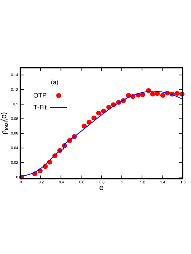
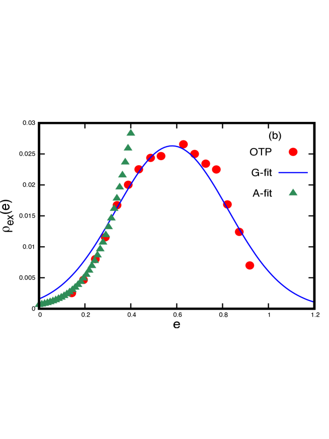
Figure 5: Vibrational DOS for OTP (with $e$ in THz units): The experimental data here is obtained by a digital scan of the figure 3 in ya21 for the reduced DOS (with $e$ in $THz$ units). All other details are same as in figure 2 except now the fits are different: ”T-Fit”=$0.23{\rm Ai}(-6.0(x-0.58))\;(1-\Theta(x-0.43))+{\Theta(x-0.43)\over\sqrt{24\pi}}{\rm exp}\left[-{(x-1.3)^{2}\over 2(0.4)}\right]+0.0015\;x^{2}$, ”G-fit”=${1\over\sqrt{460\pi}}{\rm exp}\left[-{(x-0.58)^{2}\over 2(0.06)}\right]$ and ”A-fit”=${\rm Ai}(x)=0.23\;{\rm Ai}\left[-6.0(e-0.58)\right]$. Here again both the Gaussian as well as Airy function fitting for the case (a) is slightly different from that of (b). Further Part (a) gives ${\mathcal{D}}_{b}\approx 0.0015$ but the figure 3 of ya21 gives (${\mathcal{D}}_{b}=0.109\;{THz}^{-3}$)

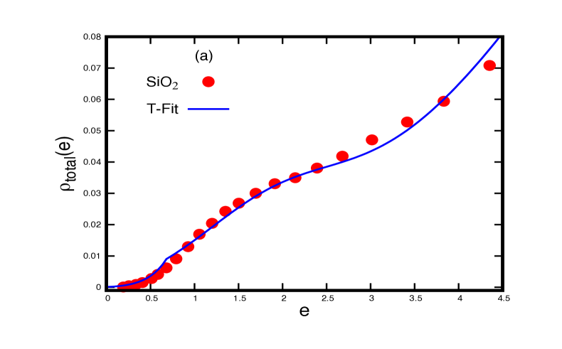
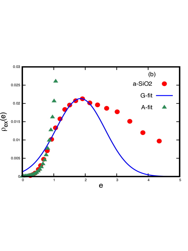
Figure 6: Vibrational DOS for a-SiO₂:(with $e$ in THz units) The experimental data here is obtained by a digital scan of the figure 12 in ya29 for reduced DOS with fits details as follows: ”T-fit”= $2.0{\rm Ai}(-2.85(x-1.85))\;(1-\Theta(x-0.7))+{\Theta(x-0.7)\over\sqrt{1000\pi}}{\rm exp}\left[-{(x-3.6)^{2}\over 2(1.6)}\right]+0.004\;x^{2}$, ”G-fit”=${1\over\sqrt{700\pi}}{\rm exp}\left[-{(x-1.85)^{2}\over 2(0.61)}\right]$ and ”A-fit”= ${\rm Ai}(x)=1.1\;{\rm Ai}\left[-2.85(e-1.85)\right]$. All other details are same as in figure 2. Here again both the Gaussian as well as Airy function fitting for the case (a) is slightly different from that of (b). The ”T-fit” in part (a) gives ${\mathcal{D}}_{b}=0.0042\;{THz}^{-3}$ which is close to ${\mathcal{D}}_{b}=0.0026\;{THz}^{-3}$ given by figure 12 of ya29 . It is not clear however why the experimental excess DOS is deviating from the Gaussian beyond $e_{gl}$ so rapidly.

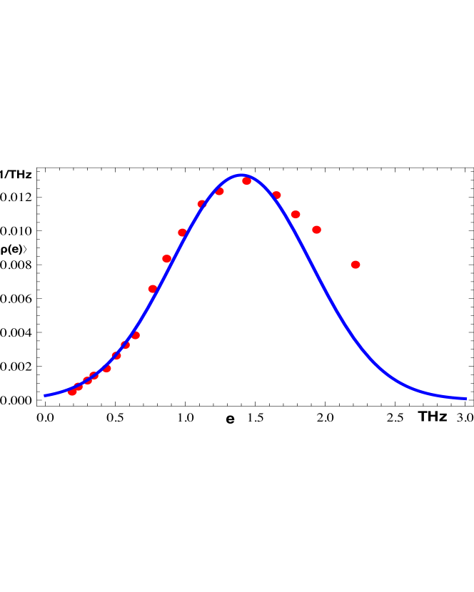
Figure 7: Vibrational DOS for another SiO₂ sample: (with $e$ in THz units) A comparison of experimental excess vibrational density of states for a glass solid, taken from buch2 (adapted from figure 6 therein), with a Gaussian fit $\rho(e)={1\over\sqrt{1800\pi}}{\rm e}^{-2(x-1.4)^{2}}$; we note that the source of experimental data here is different from figure 6. The mean $\mu=1.4$ and variance $\sigma^{2}=0.5$ of the fitted Gaussian is consistent with our theoretical prediction eq.(64). Note however, with experimental data normalized for a different energy range, the fitted Gaussian has a prefactor different from eq.(64)

The experimental studies usually present the data for reduced DOS $\langle\rho_{total}\rangle/e^{2}$. To obtain the $\langle\rho_{total}\rangle$ from the data, we use plotdigitzer software to digitally scan the figures in ya21 ; ya25 ; ya26 ; ya27 ; ya28 ), read the values for $\langle\rho_{total}\rangle/e^{2}$ for many $e$’s and convert them to $\langle\rho_{total}\rangle$ as well as excess DOS $\langle\rho_{total}\rangle-\rho_{debye}$. The converted data is displayed in figures 1-7 along with our theoretical prediction in eq.(69) and eq.(70). The latter requires a prior information about various energy scales. While theoretical prediction for $e_{ir}$ and$e_{d}$ are given by eq.(20) and eq.(21), we only have an intuitive information about $\eta_{ir}$ i.e $\eta_{ir}\approx\eta_{d}$. Using the conjecture, we have

$$e_{d}\approx 2\;e_{ir}\approx 4\;e_{bp}.$$ (73)

Eq.(21) gives the theoretical formulation for $e_{d}$ which along with above equation gives $e_{ir}$ and $e_{bp}$. Table I lists theoretical predictions for $e_{d},e_{ir}$ and $e_{bp}$ for six glasses; the required $v_{l},v_{t}$ for their determination are taken from experiments pohl ; ya21 ; ya25 ; ya26 ; ya27 ; ya28 . Here, due to a lack of data for the phonon mediated coupling strengths $\gamma_{a}$ for these glasses, $R_{b}$ can not be determined from eq.(19); we use, instead, the theoreticaly predicted relation $R_{b}=R_{0}=4R_{m}$ with $R_{m}$ as the molecular radius. To avoid cluttering the table II, the values for the edge density parameters ${\mathcal{C}}_{0}$ and ${\mathcal{B}}$ are given with the fitted function in each figure caption. We note that both $e_{ir}$ and $e_{bp}$ are indeed just fractions of one single scale i.e $e_{d}$. Using these parameters in eqs.(69, 70), the resulting distributions are then displayed in figures 1-7 alongwith their experimental counterparts.

Table II also displays the experimental values for $e_{d},e_{ir}$ and $e_{bp}$ for each of the six glass. Here the experimental value for $e_{ir}$ refers to the non-zero energy where the excess DOS effectively vanishes and experimental $e_{bp}$ corresponds to the maximum of excess DOS; both values are obtained from the experimental DOS data (displayed in figures 1-7). The table also lists the theoretical predictions for the variance $\sigma$ and energy scales $e_{gl},e_{gh}$ (the upper and lower limits for Gaussian predicted DOS given by eq.(68) and eq.(72) along with corresponding experimental values; Here the latter for $e_{gl}$ and $e_{gh}$ are taken as the energies where experimental curve deviates from the fitted Airy function and Gaussian, respectively. As indicated by table II, the relation $\sigma\approx e_{d}/12$, $e_{gh}\approx 1.9e_{bp}$ is well satisfied by all six glasses. This seems to be consistent with mizu which predicts $\omega_{bp}\approx 2\omega^{*}$; (we note $\omega^{*}$ of mizu corresponds to our $e_{ir}$).

As clear from the figure 1-6, not only the Gaussian form is consistent with experimentally observed excess DOS in the bulk of the spectrum, the behavior in the lower edge also agrees well with Airy function prediction. We also note a difference of fitted Airy parameters $c_{e},{\mathcal{B}},e_{gl}$ as well as gaussian parameters $\mu$ and $\sigma$ for total DOS (displayed in part (a)) from that of excess DOS (displayed in part (b)); this is expected due to inclusion of the Debye contribution to DOS in part (a) and its absence in part (b). Indeed the fitted parameters in part (b) are closer to their theoretical predictions.

For higher energies, we find that, a good agreement for total DOS i.e eqs.(69, 70) with experiments can be achieved only if the phonon contribution i.e Debye DOS is taken into account. Note here $e_{d}=\hbar\omega_{d}$ in principle should be obtained from eq.(21) but this requires a prior knowledge of $v_{l},v_{t}$ as well as $R_{m}$ which in turn depend on experimental conditions as well the material specific glass structure. As the latter is not available to us, we use $v_{l},v_{t}$ values from mb ; pohl and, as expected, find $e_{d}$ to be different from those mentioned in ya21 ; ya25 ; ya26 ; ya27 ; ya28 ). However the $e_{d}$-values given by fits in parts (a) of figures 1-7 and those mentioned in ya21 ; ya25 ; ya26 ; ya27 ; ya28 ) are in good agreement for Pb, Se, Glycerine and SiO₂ but differ by a factor of 2 for B₂O₃.

Figure 7 displays the comparison of experimental result for additional excitations in $SiO_{2}$ (different source than that depicted in figure 6) with a Gaussian fit; (the experimental data, shown as points, is adapted from buch by using plotdigitzer software). As figure 7 indicates, $e_{ir}\approx 3\;{\rm THz}$ and $\sigma\approx 0.5\;{\rm THz}^{-1}$ and $e_{bp}\approx 1.4\;{\rm THz}$ which is consistent with eq.(20) and eq.(65) (later gives $e_{bp}=1.5\;{\rm THz}$). Further, as metioned in buch , the maximum of excess vibrational DOS in vitreous silica is $0.013\;{\rm THz}^{-1}$. Although eq.(64) gives the maximum ${1\over\sqrt{2\pi\sigma^{2}}}\approx 0.74\;{\rm THz}^{-1}$, this discrepency seemingly arises due to different energy range used for the numerical normalization of DOS in buch .

Previous experimental studies have reported a relation between Boson peak frequency and the bulk modulus of the medium. To explore this dependence, we first note that $\rho v_{t}^{2}=G$ and $\rho\left(v_{l}^{2}-{4\over 3}v_{t}^{2}\right)=K$ with $G$ as the Bulk modulus coefficient. Substitution of these relations in eq.(20) leads to

$$e_{ir,t}={\eta_{ir,t}\;\hbar\over 2\;R_{b}}\;\sqrt{G\over\rho},\qquad e_{ir,l}={\eta_{ir,l}\;\hbar\over 2R_{b}}\;\sqrt{(K+(4/3)G)\over\rho}$$ (74)

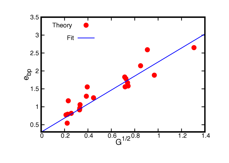
Figure 8: G-dependence of boson peak frequency (with $e_{bp}$ in THz units): The figure displays the dependence of the boson peak location $e_{bp}$ on the bulk modulus $G$ for 22 glasses listed in Tables I and II. The $G$-values for each glass are obtained from the $v_{l},v_{t}$ values listed in the tables. The figures indicates a square-root dependence of $e_{bp}$ on $G$ which is consistent with the experimental observation.

With $e_{bp}\approx e_{ir}/2$, the above eqution is consistent with the experimental observation $e_{bp}\propto\sqrt{G}$. To check the relation computationally, we compute $G$ as well as $K$ for the five glasses from the $v_{l},v_{t}$ values listed in table I and plot it with respect to $e_{bp}$ for each glass (the mean value of the fitted Gaussian in figures 1-7); the result displayed in figure 8 confirms the above relation.

The good agreement between theory and experiments encourages us to theoretically predict the $e_{bp}$ values for 18 other glasses; these are listed in table I. Here the required values for $v_{a}$ for each case are taken from pohl ; mb and $R_{b}$, given by eq.(19), is calculated in bb3 . The table I also lists the experimental data for $e_{bp}$ for a few cases which seems to agree well with our prediction for some of them. The deviation in other cases could well originate from lack of information about $v_{l},v_{t}$ values used in the experiments.

VIII Discussion and conclusion

As the VDOS of an amorphous solid has been extensively researched in past, it is relevant to compare our approach and results with previous ones. Contrary to previous theories often based on various assumptions about nature of disorder and local interactions, the many block Hamiltonian considered in this paper is based on well-known dispersion interactions of molecules within clusters of MRO length scales and a phonon mediated stress interaction among these clusters; here the randomization of Hamiltonian originates from the complicated many body interactions. With molecular clusters described as blocks, our approach is closer in spirit with those suggested in du ; sksq ; ell3 however there are some important differences e.g (i) contrary to du , the blocks described in our approach are just nanoscale partitions of amporphous solid, (ii) the clusters in du can be of varying size but the size of our blocks is fixed. We also note that the potential formulation given by eq.(4) is valid only for the phonon wavelengths larger than atomic scales. For smaller length scales i.e higher frequencies, the phonon mediated coupling of the blocks changes its form from a inverse cube dependnce on the distance to oscillatory form dl .

As the randomization of the Hamiltonian in our analysis is caused not by any structural disorder but rather due to instantaneous induced dipole interactions of the molecules (dispersion interaction), our boson peak prediction is independent of the nature of structural disorder; this is consistent with observations indicating secondary role of disorder in vibrational spectrum properties chum ; degi . A comparison with experimental data for the DOS of six amorphous solids confirms the prediction and encourages us to predict the location of boson peak for $18$ other amorphous solids (given in table I). We also find that the copuling between the blocks has no significant effect on the VDOS in the edge of the spectrum and it retains the same approximate Airy functional form as that of a single basic block. Beyond a certain energy scale (of the order of Ioffe-Regel frequency), however phonon DOS becomes significant, resulting in a small flat region for a small energy range and thereafter dominating the DOS.

Extensive investigations for the functional form of the DOS, based on various models, numerical analysis as well as experiments, indicate three characteristic frequency regimes. In low frequency regime $\omega<\omega_{0}$, with $\omega_{0}$ as a characteristic frequency of the material, the theoretical predictions are at variance and can broadly be divided into two categories: (i) the models based on soft localized vibrations predict the DOS $\rho(\omega)$ to change, with increase in frequency $\omega$, from $\omega^{4}$ (for $\omega<\omega_{0}$) to $\omega^{2}$ dependence, (for $\omega>\omega_{0}$). (ii) the models suggesting an $\omega^{2}$ behavior (e.g. those based on effective medium theories degi ; mmb ). For example, the numemerical study of mizu based on jammed particles indicates presence of both soft localized modes violating Debye-scaling as well as phonon modes following Debye scaling below $\omega_{0}$. On the contrary, effective mediium theories (EMT) based on marginal instability in amorphous solids subject to compression degi differs from mizu , indicating $\rho(\omega)\propto C\;\omega^{2}$ in regime $\omega\ll\omega_{0}$, with coefficient $C\sim(\omega^{*})^{2}$ with $\omega^{*}\sim\omega_{ir}$. Although the VDOS in Debye’s theory is also given as $\rho(\omega)\approx C_{d}\;\omega^{2}$, the difference lies in the coefficients: $C_{d}\propto(\omega^{*})^{-3/2}<C$. (We note that these powers of $\omega$ indicate only local frequency-dependence; the exact functional form of $\rho(\omega)$ is more complicated). Although our analysis indicates an Airy function behavior for the low frequency regime, a Taylor series expansion of $Ai(-{\mathcal{B}}(e-\mu))$ near $e=\mu$ however reveals a power law dependence on $e$, with dominant power varying with distance $|e-\mu|$. We note that the limit $\omega_{0}$ varies from one model to another e.g $\omega_{0}\approx 0.066\;\omega_{bp}$ in mizu and $\sim{\omega_{bp}^{2}\over\omega^{*}}$ in degi with $\omega^{*}$ is another charateristic frequency scale degi ; taking $\omega^{*}\sim\omega_{ir}$, this leads to $\omega_{0}\approx\omega_{bp}/2$. As discussed in section III, this is same as in our case with $\omega_{0}\approx e_{gl}\approx\omega_{bp}/2$.

For intermediate frequency range $\omega_{0}<\omega<\omega^{*}$, almost all models e.g srs , those based on jammed particles mizu as well as effective medium theories degi ; wyt predict a local $\omega^{2}$ dependence of DOS. Some earlier studies however have also suggested a $\omega^{3/2}$ behavior grig . Our prediction of a Gaussian form for nonphononic DOS i.e excess DOS is consistent with a local behavior $\sim\omega^{2}$ near $\omega_{bp}$; the display in figure 1-7 confirm the consistency of the Gaussian form with experimental data too.

In higher frequency range i.e $\omega>\omega^{*}$ with $\omega^{*}$ as another charactreistic frequency, the jammed particle models as well as effective mediium theories predict a constant behavior of the DOS; the latter however seems to be an artefact of the models. As discussed in previous section, our analysis also indicates a constant DOS where it results basically due to compensation of Gaussian decay of non-phononic modes by increasing number of phonoinc modes. This however survives for a very small $\omega$-range beyond $\omega_{ir}$ beyond which the typical Debye behavior of DOS starts dominating.

Besides theoretical formulation of the DOS, the present work also provides an additional insight. The Hamiltonain $H$ of the superblock is a sparse matrix in the basis space consisting of the product states of the eigenfunctions of the basic blocks. It is therefore expected to go to a many body localized phase below a system specific temperature. As this phase is believed to violate thermalization in case of an isolated system, it is also referred as a quantum ”glass” phase. This hints that an analysis of superblock Hamiltonain in NI basis of basic blocks may help us gain some insights in glass-transition phenomenon.

In the end, It is worth indicating some connections with other complex systems. The DOS described in this paper is analogous to that of the many body DOS for the ensembles of $m$ fermions with $k$-body interactions, also known as embedded ensembles, and very successful in modelling the density of states of interacting fermion systems. Another point worth noting here is following: although the Gaussian density of states here is derived in context of amorphous materials, the approach as well as the result is applicable for any sparse matrix with similar statistics of the matrix elements.

Appendix A Calculation of $\langle\left(V_{kl}\right)^{2}\rangle$

$$\langle\left(V_{kl}\right)^{2}\rangle={1\over 4}\sum_{s,t;s\not=t}\;\sum_{s^{\prime},t^{\prime};s^{\prime}\not=t^{\prime}}\;\sum_{te,te^{\prime}}\;D^{(st)}_{kl}\;D^{(s^{\prime}t^{\prime})}_{kl}\;U^{(st)}_{\alpha\beta\gamma\delta}\;U^{(s^{\prime}t^{\prime})}_{\alpha^{\prime}\beta^{\prime}\gamma^{\prime}\delta^{\prime}}\langle\;\Gamma^{(s)}_{\alpha\beta;kl}\;\Gamma^{(t)}_{\gamma\delta;kl}\;\Gamma^{(s^{\prime})}_{\alpha^{\prime}\beta^{\prime};kl}\;\;\Gamma^{(t^{\prime})}_{\gamma^{\prime}\delta^{\prime};kl}\rangle$$

(75)

where $\sum_{te,te^{\prime}}\equiv\sum_{\alpha\beta\gamma\delta}\;\sum_{\alpha^{\prime}\beta^{\prime}\gamma^{\prime}\delta^{\prime}}$. Now as the stress-matrix elements of different blocks are not correlated, we can write

$$\langle\;\Gamma^{(s)}_{\alpha\beta;kl}\;\Gamma^{(s^{\prime})}_{\alpha^{\prime}\beta^{\prime};kl}\;\Gamma^{(t)}_{\gamma\delta;kl}\;\;\Gamma^{(t^{\prime})}_{\gamma^{\prime}\delta^{\prime};kl}\rangle$$ (76)

$$= 2\langle\;\Gamma^{(s)}_{\alpha\beta;kl}\;\Gamma^{(s^{\prime})}_{\alpha^{\prime}\beta^{\prime};kl}\;\rangle.\langle\;\Gamma^{(t)}_{\gamma\delta;kl}\;\;\Gamma^{(t^{\prime})}_{\gamma^{\prime}\delta^{\prime};kl}\;\rangle$$

$$= 2\left({N^{-1}\;\omega_{u}\;\rho_{m}\;v_{a}^{2}\;\Omega_{b}}\right)^{2}\;\langle Q^{-1}_{0;s}(\omega)\rangle_{e,\omega}\;\langle Q^{-1}_{0;t}(\omega)\rangle_{e,\omega}\;\;\delta_{ss^{\prime}}\;\delta_{tt^{\prime}}$$ (77)

where the last relation is obtained by using eq.(26) and the prefactor $2$ arises from the similar contribution from pairwise combination $\Gamma^{(s)}_{\alpha\beta;kl}\;\Gamma^{(t^{\prime})}_{\gamma^{\prime}\delta^{\prime};kl}\;\rangle.\langle\;\Gamma^{(s^{\prime})}_{\alpha^{\prime}\beta^{\prime};kl}\;\;\Gamma^{(t)}_{\gamma^{\prime}\delta;kl}\;\rangle$

Substituting eq.(77) alongwith eq.(13) in eq.(75), one gets

$$\langle\left(V_{kl}\right)^{2}\rangle = {2\over(4\pi\rho_{m}v_{a}^{2})^{2}}\;\left({\omega_{u}\Omega_{b}\over N\pi}\right)^{2}\;\sum_{s,t;s\not=t}{\left(D^{(st)}_{kl}\right)^{2}\over|{\bf R_{s}}-{\bf R_{t}}|^{6}}\;W_{st}$$ (78)

with

$$W_{st} = (\rho_{m}\;v_{a}^{2})^{2}\sum_{te,te^{\prime}}\;\langle\;\kappa^{(st)}_{te}\;\kappa^{(st)}_{te^{\prime}}\;\rangle\;\;\;Y_{\alpha\beta\alpha^{\prime}\beta^{\prime}}\;Y_{\gamma\delta\gamma^{\prime}\delta^{\prime}}\;\langle Q^{-1}_{0;s}(\omega)\rangle\;\langle Q^{-1}_{0;t}(\omega)\rangle$$ (79)

As the ensemble as well as energy avearged attenuation constants of two different blocks can safely be assumed to be equal, $W_{st}$ can be written as

$$W_{st} = (\rho_{m}v_{a}^{2})^{2}\;K^{2}\;\langle Q_{0}^{-1}(\omega)\rangle_{\omega}^{2}$$ (80)

where

$$K^{2}=\sum_{te,te^{\prime}}\;Y_{\alpha\beta\alpha^{\prime}\beta^{\prime}}\;Y_{\gamma\delta\gamma^{\prime}\delta^{\prime}}\;\langle\;\kappa^{(st)}_{te}\;\kappa^{(st)}_{te^{\prime}}\;\rangle$$ (81)

with $Y_{\alpha\beta\alpha^{\prime}\beta^{\prime}}=q\;\delta_{\alpha\beta}\delta_{\alpha^{\prime}\beta^{\prime}}+\delta_{\alpha\alpha^{\prime}}\delta_{\beta\beta^{\prime}}+\delta_{\alpha\beta^{\prime}}\delta_{\beta\alpha^{\prime}}$. Here $\rho$ is the mass-density of a sub-block and $v$ is the speed of sound waves.

Substitution of eq.(80) in eq.(78) gives

$$\langle\left(V_{kl}\right)^{2}\rangle = 2\left({N^{-1}\;\omega_{u}\;K}\right)^{2}\;\;\langle Q_{0}^{-1}(\omega)\rangle_{\omega}^{2}\;\;C_{kl}$$ (82)

with $C_{kl}$ given by eq.(32) and

$$K^{2}=(8/3)[-3+4s+16q(q+s+qs-1)]=122.1.$$ (83)

Here the $2nd$ equality above follows from the typical values of $q\equiv 1-{v^{2}_{t}\over v^{2}_{l}}\simeq 0.6$ and $s\equiv{{\rm Im}\chi_{l}\over{\rm Im}\chi_{t}}\simeq 2.6$.

Appendix B Calculation of $C_{kl}$

Following from eq.(14), $D^{(st)}_{kl}=1$ for all those $(k,l)$ pairs which differ, if at all, only in contributions from the specific blocks $s$ and/or $t$ and is zero otherwise. For example, if $|k\rangle,|l\rangle$ differ in the contributions from a single block, say ”p”, that is, if $k_{p}\not=l_{p}$ with $p\not=s,t$ then $D^{(st)}_{kl}=0$. But $D^{(st)}_{kl}=1$ if $p=s\;{\rm or}\;t$. As a consequence, eq.(32) gives, for a pair $|k\rangle,|l\rangle$ forming a $j$-plet,

$$C_{kl} = \;\delta_{kl}\;\;{1\over 4\pi^{2}}\;\sum_{s,t;s\not=t}{\Omega_{b}^{2}\over|\;{\bf R_{s}}-{\bf R_{t}}\;|^{6}}\hskip 21.68121pt{\rm for}\;j=0$$ (84)

$$= {1\over 4\pi^{2}}\;\sum_{t}\;{\Omega_{b}^{2}\over|\;{\bf R_{s}}-{\bf R_{t}}\;|^{6}}\hskip 43.36243pt{\rm for}\;j=1,\;k_{s}\not=l_{s}\;{\rm or}\;k_{t}\not=l_{t}$$ (85)

$$= {1\over 4\pi^{2}}\;{\Omega_{b}^{2}\over|\;{\bf R_{s}}-{\bf R_{t}}\;|^{6}}\hskip 57.81621pt{\rm for}\;j=2,\;k_{s}\not=l_{s}\;{\rm and}\;k_{t}\not=l_{t}$$ (86)

$$= 0\hskip 144.54pt{\rm for}\;\;j>2,$$ (87)

where $"s"$ in eq.(85) refers to the block whose eigenfunction contribution to $|k\rangle$ and $|l\rangle$ (as they form $1$-plets) is different. Note the subscripts $k$ and $l$ are not explicitely present on the right side of eq.(85) and therefore $C_{kl}$ for all $k,l$ pairs which differ in the contribution from the same block ”s” will be equal. Similarly $"s"$ and $"t"$ in eq.(86) correponds to two blocks whose contributons (eigenfunctions) to $|k\rangle$ are diiferent from the ones to $|l\rangle$ (as they form $2$-plets). Again the subscripts $k$ and $l$ are absent on right side of eq.(86) and therefore $C_{kl}$ for all $k,l$ pairs which differ in the contribution from the same blocks ”s,t” will be equal.

Following from the above, $C_{kl}$ for $k,l$ pairs forming $2$-plets are quite small as compared to those forming $0$ and $1$-plets.

As the case of a $k,l$ pair forming a $0$-plet is possible only if $|k\rangle=|l\rangle$, it corresponds to a diagonal matrix element. This gives the total number of $0$-plets as the size of NI basis i.e $N^{g}$ with $N$ as the number of single block energy levels and $g$ as the number of basic blocks in the superblock. Also all clear from eq.(84), all $C_{kk}$ are equal i.e $C_{kk}=C_{0}$ where

$$C_{0} \equiv {1\over 4\pi^{2}}\;\sum_{s,t;s\not=t}\;{\Omega_{b}^{2}\over|\;{\bf R_{s}}-{\bf R_{t}}\;|^{6}}\approx g\;d_{0}$$ (88)

where $d_{0}$ is a dimensionless constant. As the dominant contribution to $\sum_{s,t}$ comes from the neighboring blocks, $d$ can be estimated as $d_{0}\sim{z\over 144}$ (assuming basic block of spherical shape with $\Omega_{b}=(4\pi/3)R_{b}^{3}$ and $R_{b}\approx|R_{s}-R_{t}|/2$ for two neighboring blocks with $z$ as the number of nearest neighbors of a given block). The above implies

$$\sum_{k,l\;\epsilon\;0-plet}C_{kl}=\sum_{k}C_{kk}=N^{g}\;C_{0}$$ (89)

The total number of $k,l$ pairs forming $1$-plets is $g(N-1)N^{g}$ and these will arise from all possible $s,t$ pairs chosen out of $g$ basic blocks. But only a total of $N^{g}(N-1)$ possible pairs of such eigenvectors $|k\rangle,|l\rangle$ correspond to a same block $s$; from eq.(86), $C_{kl}$ for all such $k,l$ pairs is equal. As a consequence, we have

$$\sum_{k,l\;\epsilon\;1-plet}C_{kl} = {N^{g}(N-1)\over 4\pi^{2}}\;\sum_{s,t;s\not=t}\;{\Omega_{b}^{2}\over|\;{\bf R_{s}}-{\bf R_{t}}\;|^{6}}=N^{g}\;(N-1)\;C_{0}$$

The total number of $|k\rangle,|l\rangle$ basis pairs forming $2$-plets is ${g(g-1)\over 2}(N-1)^{2}N^{g}$, arising from all possible basic block pairs $s,t$ but only a total of $N^{g}\;(N-1)^{2}$ pairs of them correspond to a same pair of blocks $s,t$; from eq.(86), $C_{kl}$ for all such $k,l$ pairs, which arise from same block-pair $s,t$, is equal. As a consequence, we have

$$\sum_{k,l\;\epsilon\;2-plet}C_{kl} = {N^{g}(N-1)^{2}\over 4\pi^{2}}\;\sum_{s,t;s\not=t}\;{\Omega_{b}^{2}\over|\;{\bf R_{s}}-{\bf R_{t}}\;|^{6}}=N^{g}\;(N-1)^{2}\;C_{0}$$

From, eqs.(89, LABEL:cd1, LABEL:cd2), we have

$$\sum_{kl}C_{kl} = \sum_{k}C_{kk}+\sum_{k,l\;\epsilon\;(g-1)-plet}C_{kl}+\sum_{k,l\;\epsilon\;(g-2)-plet}C_{kl}$$ (92)

$$= \left[1+(N-1)+(N-1)^{2}\right]\;N^{g}\;C_{0}$$

$$\approx N^{g+2}\;\;C_{0}$$

Appendix C Calculation of $\langle\left(V_{kl}\right)^{n}\rangle$

$$\langle\left(V_{kl}\right)^{n}\rangle=\sum_{S}\;\sum_{te_{1}\ldots te_{n}}\left(\prod_{p=1}^{n}D^{(s_{p}t_{p})}_{kl}\;U^{(s_{p}t_{p})}_{\alpha_{p}\beta_{p}\gamma_{p}\delta_{p}}\right)\;F_{st}$$ (93)

where $\sum_{S}\equiv\sum_{s_{1},t_{1}\atop s_{1}\not=t_{1}}\ldots\sum_{s_{n},t_{n}\atop s_{n}\not=t_{n}}$ and $\sum_{te_{1}\ldots te_{n}}\equiv\sum_{\alpha_{1}\beta_{1}\gamma_{1}\delta_{1}}\;\ldots\sum_{\alpha_{n}\beta_{n}\gamma_{n}\delta_{n}}$ and

$$F_{st}=\langle\;\Gamma^{(s_{1})}_{\alpha_{1}\beta_{1};kl}\;\Gamma^{(t_{1})}_{\gamma_{1}\delta_{1};kl}\;\Gamma^{(s_{2})}_{\alpha_{2}\beta_{2};kl}\;\Gamma^{(t_{2})}_{\gamma_{2}\delta_{2};kl}\ldots\Gamma^{(s_{n})}_{\alpha_{n}\beta_{n};kl}\;\Gamma^{(t_{n})}_{\gamma_{n}\delta_{n};kl}\rangle$$ (94)

Here again, the pairwise correlations between the stress-matrix elements of different blocks are negligible and only those between same blocks are relevant. For example, for $n=2m$, $F_{st}$ becomes

$$F_{st} = \prod_{i,j=1}^{2m}\langle\;\Gamma^{(s_{i})}_{\alpha_{i}\beta_{i};kl}\;\Gamma^{(s_{j})}_{\alpha_{j}\beta_{j};kl}\;\rangle.\langle\;\Gamma^{(t_{i})}_{\gamma_{i}\delta_{i};kl}\;\;\Gamma^{(t_{j})}_{\gamma_{j}\delta_{j};kl}\;\rangle$$ (95)

$$= \left({N^{-1}\;\omega_{u}\;\rho_{m}\;v_{a}^{2}\;\Omega_{b}}\right)^{2m}\;\prod_{i,j=1}^{2m}\left(\langle Q^{-1}_{0;s_{i}}(\omega)\rangle_{\omega}\;\langle Q^{-1}_{0;t_{i}}(\omega)\rangle_{\omega}\;\delta_{s_{i}s_{j}}\;\delta_{t_{i}t_{j}}\right)$$ (96)

where the $2nd$ equality is obtained by using eq.(26) respectively.

The presence of terms $\delta_{s_{i}s_{j}}\delta_{t_{i}t_{j}}$ in eq.(96) ensures contribution to $\langle\left(V_{kl}\right)^{2m}\rangle$ only from those terms in the sum $\sum^{S}$ which correspond to pairwise combinations among $s_{1}s_{2}\ldots s_{2m}$ (and among $t_{1}t_{2}\ldots t_{2m}$). In absence of any other condition (except $s_{i}\not=t_{i}$) on pairwise combinations, the number of such combinations can be ${}^{2m}C_{2}=(2m-1)!!$. Thus one can replace $\sum^{S}$ by the sum over even indices only: $\sum^{S}=(2m-1)!!\;\sum_{s_{2},t_{2},s_{4},t_{4},\ldots,s_{2m},t_{2m}\atop s_{2}\not=t_{2},s_{4}\not=t_{4},\ldots,s_{2m}\not=t_{2m}}$. As each such combination has same contribution, one can write

$$\langle\left(V_{kl}\right)^{2m}\rangle = (2m-1)!!\;\left({\omega_{u}\;\Omega_{b}\over\pi N}\right)^{2m}\sum_{s_{2},t_{2},s_{4},t_{4},\ldots,s_{2m},t_{2m}\atop s_{2}\not=t_{2},s_{4}\not=t_{4},\ldots,s_{2m}\not=t_{2m}}\prod_{p=2}^{2m}\;{D^{(s_{p}t_{p})}_{kl}\;W_{s_{p}t_{p}}\over({\bf R_{s_{p}}}-{\bf R_{t_{p}}})^{6}}$$ (97)

with $W_{s_{p}t_{p}}$ is same as eq.(79).

The summation and product over terms in the above equation can be rearranged to write

$$\langle\left(V_{kl}\right)^{2m}\rangle = (2m-1)!!\;\left({\omega_{u}\;\Omega_{b}\over\pi N}\right)^{2m}\;\prod_{p=2}^{2m}\left(\sum_{s_{p},t_{p}\atop s_{p}\not=t_{p}}\;{D^{(s_{p}t_{p})}_{kl}\;W_{s_{p}t_{p}}\over({\bf R_{s_{p}}}-{\bf R_{t_{p}}})^{6}}\right)$$ (98)

Substitution of eq.(80) and eq.(81) in eq.(97) gives

$$\langle\left(V_{kl}\right)^{2m}\rangle = (2m-1)!!\;\left({\omega_{u}\;\Omega_{b}\over\pi N}\right)^{2m}\;\;\langle Q_{0}^{-1}(\omega)\rangle_{\omega}^{2m}\;\prod_{p=2}^{2m}\left(\sum_{s_{p},t_{p}\atop s_{p}\not=t_{p}}\;{D^{(s_{p}t_{p})}_{kl}\over({\bf R_{s_{p}}}-{\bf R_{t_{p}}})^{6}}\right)$$ (99)

$$= (2m-1)!!\;\left({\omega_{u}\;\Omega_{b}\over\pi N}\right)^{2m}\;\;\langle Q_{0}^{-1}(\omega)\rangle_{\omega}^{2m}\;\left(C_{kl}\right)^{2m}$$ (100)

$$= (2m-1)!!\;\langle\left(V_{kl}\right)^{2}\rangle^{m}$$ (101)

which is same as eq.(36).

Table 2: Comparison of Theoretically predicted range and location of excess VDOS with experimental data (all energy scales in THz units): Based on inelastic neutron and Raman scattering, the studies ya26 ; ya21 ; ya27 ; ya28 describe the experimental behavior for excess VDOS for five materials, namely, Selenium, $B_{2}O_{3}$, orthoterphenayl, Polybutadiene (PB), and Glycerol in the energy range upto $6-8\;{\rm mev}$ ($1\;{\rm THz}=4.136\;{\rm meV}=6.64\times 10^{-22}\;{\rm Joules}$). Using the Plotdigitzer software, we digitally scan the figures in ya26 ; ya21 ; ya27 ; ya28 and display the experimental data for total DOS as well as excess DOS in figures 1-7 along with a numerical fitting in each case (using standard GNU software). This table gives the fitted and theoretical values of all the relevant energy scales in case of excess DOS (parts (b) of figures 1-7) i.e $e_{d}$ (Debye, eq.(21)), $e_{ir}$ (Ioffe-Regel, eq.(20)), $e_{bp}$ (boson peak, eq.(65)), $\sigma$ (variance, eq.(66)), $e_{gl}$ and $e_{gh}$ (lower eq.(72) and upper limits eq.(68) of Gaussian VDOS). We note that $R_{b}$ in this case can not be determined from eq.(19) (due to unavailability of the experiemental data for the phonon mediated coupling strengths $\gamma_{a}$). As the only alternative available left, we use the theoreticaly predicted value for $R_{b}$ i.e $R_{b}=R_{0}=4R_{m}$ with $R_{m}$ as the molecular radius: $R_{m}={M\over\rho_{m}N_{a}}$ with $M,\rho,N_{a}$ as the mass of the basic structural unit, mass density and Avogrado numberbb3 . The values of $v_{l},v_{t}$ and $\rho_{m}$ for Se, PB, B₂O₃, SiO₂ are taken from mb ; pohl and $M$ from bb2 . But in case of OTP (Orthoterphenyl), $v_{l},v_{t}$ are taken from hw and $M,\rho_{m}$ from PubChem. For Glycerine, $v_{l},v_{t}$ are taken from lya . Here the deviations of theoretical predictions from experiments in some cases can be attributed to lack of exact information about the the basic structural unit participating in the dispersion intercations within a basic block and thereby its mass $M$ bb1 ; bb2

.

Ind.	Glass	$M\atop{gm\over mol}$	${\rho\atop\;{gm\over cm^{3}}}$	${R_{m}\atop\AA}$	${v_{l}\atop{km\over sec}}$	${v_{l}\atop{km\over sec}}$	${e_{d}\atop th.}$	${e_{d}\atop exp}$	${e_{ir}\atop th.}$	${e_{ir}\atop fit}$	${\sigma\atop th.}$	${\sigma\atop fit}$	${e_{bp}\atop th.}$	${e_{bp}\atop fit}$	${e_{gl}\atop th.}$	${e_{gl}\atop fit}$	${e_{gh}\atop th.}$	${e_{gh}\atop fit}$
1	Se	78.96	4.30	1.94	2.00	1.05	3.66	3.68	1.83	1.6	0.31	0.27	0.92	0.66	0.48	0.36	1.75	1.1
2	PB	55.15	0.93	2.86	3.02	1.46	3.46	3.40	1.73	1.69	0.29	0.31	0.87	0.87	0.46	0.43	1.47	1.45
3	B2O3	69.62	1.80	2.48	3.47	1.91	5.18	8.07	2.59	3.87	0.43	0.95	1.30	1.81	0.69	0.68	2.46	2.41
4	Glyc.	92.09	1.42	2.95	3.52	1.85	4.23	6.77	2.12	2.66	0.35	0.38	1.06	1.38	0.57	-	2.01	2.01
5	OTP	230.3	1.16	1.99	2.94	1.37	4.69	4.35	2.35	1.2	0.39	0.25	1.17	0.58	0.62	0.34	1.03	0.9
6	SiO2	120.09	2.20	2.51	5.80	3.80	10.06	15.11	5.03	4.0	0.84	0.78	2.52	1.85	1.33	0.91	4.9	2.2

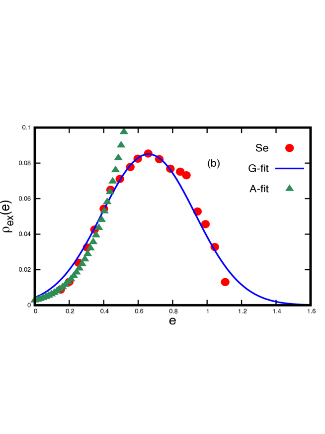
Figure 1: Vibrational DOS for Se (with $e$ in THz units): The figure illustrates a comparison of theoretical prediction (solid line) with experimental data (filled circles) (latter obtained by a digital scan of the figure 3 in ya25 for the total DOS using the Plotdigitzer software): (a) total vibrational DOS $\rho_{total}\equiv\langle\rho_{total}(e)\rangle$ with $e=\hbar\omega$, (b) excess vibrational DOS $\rho_{ex}\equiv\langle\rho_{total}(e)\rangle-\rho_{Debye}(e)$ where $\rho_{Debye}(e)={\mathcal{D}}_{b}\;e^{2}$. The part (a) shows a theoretical fitting of eq.(70) (”T-fit” = $0.2\;{\rm Ai}\left[-9.5(e-0.35)\right]\;(1-\Theta(e-0.5))+{\Theta(e-0.5)\over\sqrt{6\pi}}{\rm exp}\left[-{(e-1.3)^{2}\over 2(0.5)}\right]+0.008e^{2}$). Here $\Theta(x-a)$ refers to Heavyside step function: $\Theta(x-a)=0$ for $x<a$ and $\Theta(x-a)=1$ for $x>a$. The part (b) displays two fits i.e a Gaussian (”G-fit” = ${1\over\sqrt{44\pi}}{\rm exp}\left[-{(e-0.66)^{2}\over 2(0.073)}\right]$ and an Airy function (”A-fit”=$0.5\;{\rm Ai}\left[-4.7(e-0.66)\right]$ ) separately (to verify that the DOS in the lower edge indeed behaves as an Airy function). We note that the fitting parameters for the case (a) are different from that of (b). This is because while in part (a), ${\mathcal{D}}_{b}=0.008\;{THz}^{-3}$, is obtained by fitting the experimental data, the excess DOS in part (b) is obtained by substracting the Debye DOS data given in figure 3 of ya25 (the experimental data in the latter gives ${\mathcal{D}}_{b}=0.18\;{THz}^{-3}$).

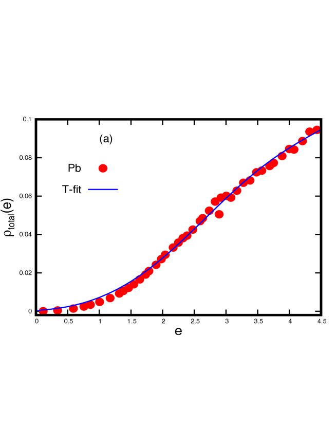
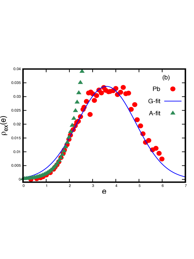
Figure 2: Vibrational DOS for Pb (with $e$ in mev units): The experimental data here is obtained by a digital scan of the figure 12 in ya27 for the reduced DOS ${\langle\rho(e)\rangle\over e^{2}}$ (with $e$ in $mev$ units) and then using it to obtain (a) $\langle\rho(e)\rangle$ and (b) $\rho_{excess}=\langle\rho(e)\rangle-{\mathcal{D}}_{b}\;e^{2}$. Here ”T-fit”=$0.4{\rm Ai}(-1.2(x-3.6))\;(1-\Theta(x-0.5))+{\Theta(x-0.5)\over\sqrt{340\pi}}{\rm exp}\left[-{(x-3.6)^{2}\over 2(1.6)}\right]+0.0035\;x^{2}$ and ”G-fit”=${1\over\sqrt{280\pi}}{\rm exp}\left[-{(x-3.6)^{2}\over 2(1.6)}\right]$ and ”A-fit”=${\rm Ai}(x)=0.4\;{\rm Ai}\left[-1.2(e-3.6)\right]$. All other details are same as in figure 2. We note that here the fitting parameters for case (a) are in excellent agreement with those of (b). Also note that fitting of the experimental data in part (a) gives ${\mathcal{D}}_{b}=0.0035\;{mev}^{-3}$ which is very close ${\mathcal{D}}_{b}=0.0032\;{mev}^{-3}$ to that given by figure 12 of ya27 .

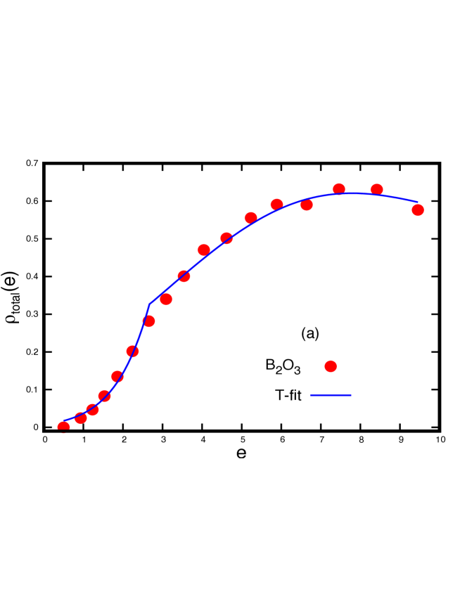
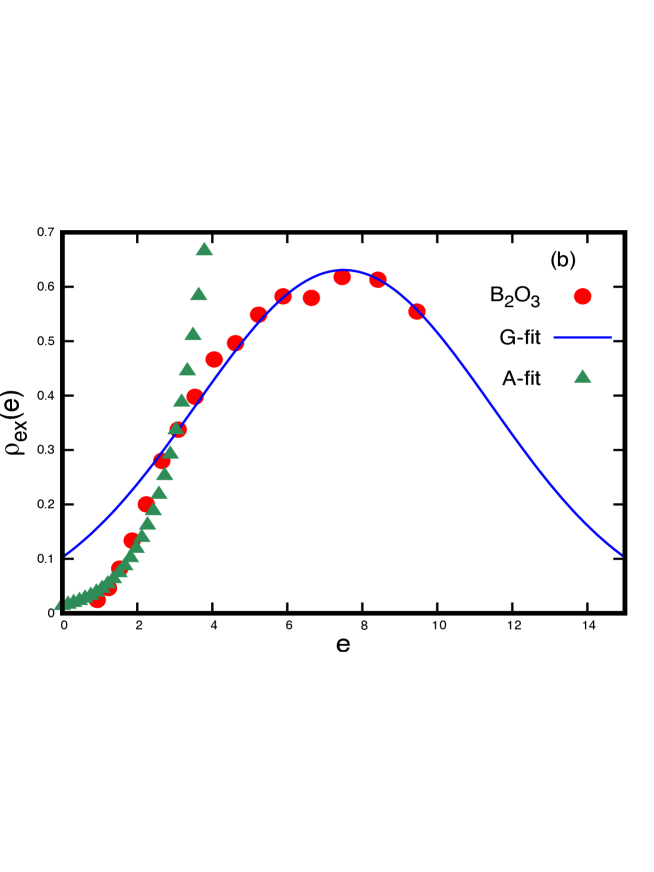
Figure 3: Vibrational DOS for B₂O₃ (with $e$ in mev units): The experimental data here is obtained by a digital scan of the figure 12 in ya26 for reduced DOS with fits details as follows: ”T-fit”=$26.7{\rm Ai}(-0.7(x-6.5))\;(1-\Theta(x-2.7))+{\Theta(x-2.7)\over\sqrt{1.3\pi}}{\rm exp}\left[-{(x-6.5)^{2}\over 2(15.5)}\right]+0.0035\;x^{2}$, ”G-fit”=${1\over\sqrt{280\pi}}{\rm exp}\left[-{(x-7.5)^{2}\over 2(15.5)}\right]$ and ”A-fit”=${\rm Ai}(x)=21.5\;{\rm Ai}\left[-0.56(e-7.5)\right]$. All other details are same as in figure 2. Here again both the Gaussian as well as Airy function fitting for the case (a) is slightly different from that of (b). Further ”T-fit” in part (a) gives ${\mathcal{D}}_{b}=2.9\times 10^{-4}\;{mev}^{-3}$ which is close ${\mathcal{D}}_{b}=2.43\times 10^{-4}\;{mev}^{-3}$ to given by figure 4 of ya28

.

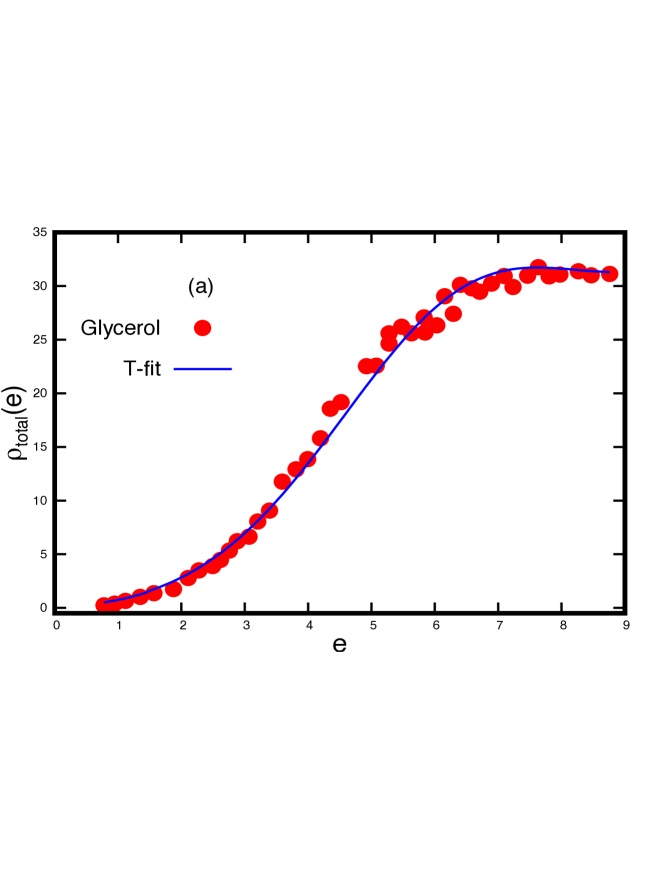
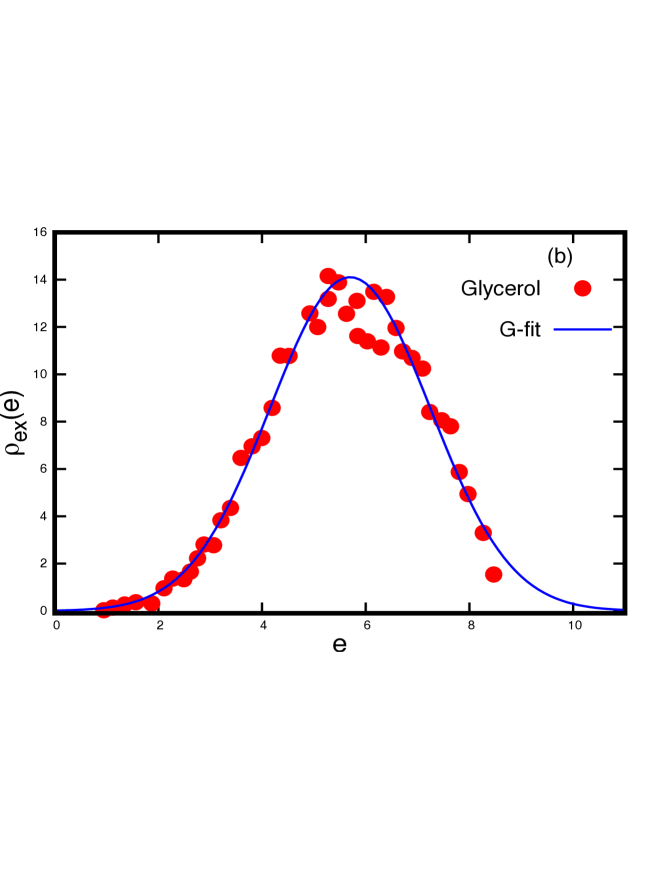
Figure 4: Vibrational DOS for Glycerol (with $e$ in mev units): The experimental data here is obtained by a digital scan of the figure 4 in ya28 for reduced DOS with fits details as follows: ”T-fit”=$6.4{\rm Ai}(-1.0(x-2.5))\;(1-\Theta(x-1.5))+{\Theta(x-1.5)\over\sqrt{340\pi}}{\rm exp}\left[-{(x-6.4)^{2}\over 2(4.1)}\right]+0.29\;x^{2}$ and ”G-fit”= ${1\over\sqrt{0.0016\pi}}{\rm exp}\left[-{(x-5.7)^{2}\over 2(2.4)}\right]$, referred as ”G-fit”. All other details are same as in figure 2. We note here the validity of a Gaussian behaviour in the full range of part (b). Here again the Gaussian fitting for the case (a) is slightly different from that of (b). Further ”T-fit” in part (a) gives ${\mathcal{D}}_{b}=2.9\times 10^{-4}\;{mev}^{-3}$ which is close ${\mathcal{D}}_{b}=2.43\times 10^{-4}\;{mev}^{-3}$ to given by figure 4 of ya28

.

.

References

• (1) U. Buchenau, N. Nucker and A.J. Dianoux, Phys. Rev. Lett., 53, 2316, (1984).
• (2) V. K. Malinovsky, V. N. Novikov, P.P. Parashin, A.P. Solokov and M.G. Zemlyanov, Europhys. Lett., 11, 43 (1990).
• (3) Due to intense interest, many research papers have been published over the years on the topic and it is not feasible to include all of them here. For example, many references on the topic can be found in Dynamics of Disordered Materials II., edited by A.J. Dianoux, W. Petry and D. Richter (North-Holland, Amsterdam, 1993).
• (4) S.R.Elliott, Europhys. Lett. 19, 201 (1992).
• (5) U. Bucheanau, Y. M. Galperin, V. Gurevich, D. Parashin, M. Ramos and H. Schober, Phys. Rev. B 46, 2798, (1992); 43, 5039, (1991).
• (6) V.G.Karpov, M.I.Klinger, F.N.Ignatiev, Sov. Phys. JETP 57, 439, (1983).
• (7) V. Gurevich, D. Parashin and H. Schrober, Phys. Rev. B, 67, 094203, (2003).
• (8) D. Parashin, H. Schrober and V. Gurevich, Phys. Rev. B 76, 064206, (2007).
• (9) B. Ruffle, D.A.Parashin, E.Courtens and R. Vacher, arXiv:0711.0461
• (10) W. Schirmacher, G. Diezemann and C. Ganter, Phys. Rev. Lett., 81, 136, (1998).
• (11) S N Taraskin and S R Elliott, Phys Rev B 61,12031, (2000); S N Taraskin, Y.L.Loh, G.Natrajan and S R Elliott, Phys Rev Lett 86, 1255, (2001).
• (12) W. Schirmacher, Europhys. Lett. 73, 892, (2006); A. Maruzzo, W. Schirmacher, A. Fratalocchi and G. Ruocco, Sci. Rep., 3, 1407, (2013).
• (13) T.S. Grigera, V. Martin-Mayor, G. Parisi, P. Verrocchio, Nature 422 (2003) 289; G. Parisi, J. Phys.: Condens. Matter 15 (2003) S765, and references therein.
• (14) W. Schirmacher, G. Ruocco and T. Scopigno, Phys. Rev. Lett. 98, 025501, (2007).
• (15) V. Gurarie and A. Altland, Phys. Rev. Lett. 94, 245502, (2005).
• (16) M. Wyart, Europhys. Lett. 89, 64001, (2010).
• (17) M. Wyart, S. R. Nagel and T A Witten, Europhys. Lett. 72, 486, (2005).
• (18) M. Wyart, S. R. Nagel and T A Witten, Phys. Rev. E. 72, 051306, (2005).
• (19) E. DeGiuli, A. Laversanne-Finot, G. During, E. Lerner and M. Wyart, Soft Matter, 10, 5628, (2014).
• (20) H. Mizuno, H. Shiba and A. Ikeda, PNAS 114, E9767, (2017).
• (21) M.L.Manning and A J Liu, 109, 36002, (2015).
• (22) E. Stanifer, P.K.Morse, A.A.Middleton and M.L.Manning, Phys. Rev. E, 98, 042908, (2018).
• (23) Y.M.Beltukov and D.A.Parashin, Physics of the solid state, 53, 151, (2011).
• (24) M. Baggioli and A. Zaccone, Phys. Rev. Research 1, 012010(R), (2020); M. Baggioli, R. Milkus, and A. Zaccone, Phys. Rev. E 100, 062131, (2019).
• (25) C S Ohern, L E Silbert, A J Liu and S R Nagel, Phys. Rev. E, 68, 011306, (2003).
• (26) V. Lubchenko and P. G. Wolynes, Proc. Natl. Acad. Sci. USA 100, 1515 (2003).
• (27) E. Duval, A. Boukenter, T. Achibat, J. Phys. Condens. Matter 2, 10227, (1990).
• (28) V K Malinovsky, V N Novikov and A P sokolov, Phys. Lett. A, 153, 63, (1991).
• (29) A. P. Sokolov, A. Kisliuk, M. Soltwisch, and D. Quitmann Phys. Rev. Lett. 69, 1540 (1992).
• (30) S. Franz, G. Parisi, P. Urbani and F. Zamponi, PNAS, 112, 14359, (2015).
• (31) P. Shukla, arXiv:2008.12960.
• (32) P. Shukla, arXiv:2009.00556.
• (33) P. Shukla, arXiv:2101.00492
• (34) G. Monaco and V. M. Giordano, PNAS.0808965106.
• (35) J. Israelachvili, Chapter 11, Intermolecular and Surface Forces, 3rd ed. Academic Press, (2011).
• (36) A.J.Stone, The theory of intermolecular forces, Oxford scholarship online, Oxford university Press, U.K. 2015.
• (37) C. Argento, A. Jagota, W.C. Carter, J. Mech. Phys. Solids 45, 1161, (1997).
• (38) R.M. Meeking, J. Colloid Interface Sci. 199, 187, (1998).
• (39) L.H.He, J. Mech. Phys. Solids 61, 1377, (2013).
• (40) D. Vural and A.J.Leggett, J. Non crystalline solids, 357, 19, 3528, (2011).
• (41) Z. Dee and A. J. Leggett, arXiv: 1510:05528v1.
• (42) A. J. Leggett and D. Vural, J. Phys. Chem. B., 42,117, (2013).
• (43) J. Joffrin and A. Levelut, Jou.de. Physique, 36, 811, (1975).
• (44) D. A. Parashin, Phys. Rev. B, 49, 9400, (1994).
• (45) H-J Stockmann, Quantum Chaos: an introduction, Cambridge univ. Press (1999) (see page 79).
• (46) L. Isserlis, Biometrika, 12, 134, (1918).
• (47) G. J. Rodgers and A. J. Bray, Phys. Rev. B, 37, 3557, (1998).
• (48) A. Khorunzhy and G. J. Rodgers, J. Math. Phys. 38, 3300 (1997).
• (49) R.C Jones, J M Kosterlitz and D J Thouless, J. Phys. A: Math. Gen., 11, 3,1978.
• (50) E. Lerner, G. Düring, and E. Bouchbinder, Phys. Rev. Lett., 117, 035501, (2016).
• (51) A. I. Chumakov et al., Phys. Rev. Lett. 106, 225501 (2011).
• (52) Y. Wang, L. Hong, Y. Wang, W. Schirmacher and J. Zhang, Phys. Rev. B 98, 174207 (2018).
• (53) Y. Nie, H. Tong, J. Liu, M. Zu, N. Xu, Front. Phys. 12, 126301 (2017)
• (54) T.A.Brody, J.Flores, J.B.French, P.A.Mello, A. Pandey and S.S.M Wong, Rev. Mod. Phys., 53, 1981.
• (55) R.H. Stolen, Phys.Chem.Glasses, 11, 83, (1970).
• (56) R.J. Nemanich, Phys.Rev.B, 16, 1665, (1977).
• (57) V.N. Novikov, and A.P. Sokolov, Sol.State Comm., 77, 243, (1991).
• (58) J.L. Prat, F. Terki, and J. Pelous, Phys.Rev.Lett., 77, 755, (1996).
• (59) K.G. Breitschwerdt, and S. Gut, Proc. 12 Intern. Conf. on acoustic, Toronto, G2-6, (1986).
• (60) V A Ryzhov, Phys Astron Int J. 3, 123, (2019).
• (61) D. A. Parashin and C. Laermans, Phys. Rev. B 63, 132203, (2001).
• (62) S. Perticaroli, J. D. Nickels, G. Ehlers and A. P. Sokolov, Biophysical Journal, 106, 2667, (2014).
• (63) S.N. Yannopoulos, K.S. Andrikopoulos, G. Ruocco, J. Non-Cryst. Sol. 352, 4541, (2006).
• (64) A. Tolle, H. Zimmermann, F. Fujara, W. Petry, W. Schmidt, H. Schober, J. Wuttke, Eur. Phys. J. B 16 , 73, (2000).
• (65) W.A. Phillips, U. Buchenau, N. Nucker, A. J.Dianoux, W. Petry, Phys. Rev. Lett. 63, 2381, (1989).
• (66) D. Engberg, A. Wischnewski, U. Buchenau, L. Borjesson, A.J. Dianoux, A.P. Sokolov, L.M. Torell, Phys. Rev. B 58, 9087, (1998).
• (67) R. Zorn, A. Arbe, J. Colmenero, B. Frick, D. Richter, U. Buchenau, Phys. Rev. E 52, 781, (1995).
• (68) J. Wuttke, W. Petry, G. Goddens, F. Fujara, Phys. Rev. E 52, 4026, (1995).
• (69) A. Wischnewski, U. Buchenau, A.J. Dianoux, W. A. Kamitakahara, J. L. Zarestky, Phys. Rev. B 57, 2663, (1998).
• (70) H. Mizuno, S. Mossa and J.-L. Barrat, arXiv:1308.5135, (2013).
• (71) R. P. Hermann, R. JIn, W. Schweika, F. Grandjean, D. Mandrus, B. C. Sales, G.J. Long, Phys. Rev. Lett. 90, 135505, (2003).
• (72) R.O.Pohl, X.Liu and E.Thompson, Rev. Mod. Phys. 74, 991, (2002).
• (73) J.F. Berret and M. Meissner, Z. Phys. B-Condensed Matter 70, 65, (1988).
• (74) P. Shukla, to be submitted.
• (75) Y. Higashigaki and C.H. wang, J. Chem. Phys. 74, 3175, (1981).
• (76) A.G.Lyapin, RSC ADV,7 33278, (2017).