Exact Critical Casimir Amplitude of Anisotropic Systems from Conformal Field Theory and Self-Similarity of Finite-Size Scaling Functions in $d\geq 2$ Dimensions

Abstract

The exact critical Casimir amplitude is derived for anisotropic systems within the $d=2$ Ising universality class by combining conformal field theory (CFT) with anisotropic $\varphi^{4}$ theory. Explicit results are presented for the general anisotropic scalar $\varphi^{4}$ model and for the fully anisotropic triangular-lattice Ising model in finite rectangular and infinite strip geometries with periodic boundary conditions (PBC). These results demonstrate the validity of multiparameter universality for confined anisotropic systems and the nonuniversality of the critical Casimir amplitude. We find an unexpected complex form of self-similarity of the anisotropy effects near the instability where weak anisotropy breaks down. This can be traced back to the property of modular invariance of isotropic CFT for $d=2$. More generally, for $d>2$ we predict the existence of self-similar structures of the finite-size scaling functions of $O(n)$-symmetric systems with planar anisotropies and PBC both in the critical region for $n\geq 1$ as well as in the Goldstone-dominated low-temperature region for $n\geq 2$.

Fluctuation-induced thermodynamic forces are ubiquitous in confined condensed matter systems kardar . They exist in both isotropic systems such as fluids, superfluids, and binary liquid mixtures krech ; gambassi as well as in anisotropic systems such as liquid crystals kardar ; ajdari1991 , superconductors wil-1 , and compressible solids dohm2011 . Near a critical point, so-called critical Casimir forces krech ; gambassi arise from long-range critical fluctuations, which generate a universal finite-size critical behavior that can be classified in universality classes with universal critical exponents priv . Within a universality class there exist subclasses dohm2008 ; dohm2018 of isotropic and weakly anisotropic $d$-dimensional systems – the latter have $d$ independent nonuniversal correlation-length amplitudes in $d$ principal directions. While the Casimir force amplitude at criticality is widely believed to be a universal quantity affleck ; bloete ; priv ; pri ; krech ; gambassi ; dubail ; privman1990 , this is not valid for weakly anisotropic $O(n)$-symmetric systems with an $n$-component order parameter in $2<d<4$ dimensions cd2004 ; dohm2006 ; dohm2008 ; kastening-dohm ; dohm2018 . Furthermore, low-temperature Casimir forces due to Goldstone modes dohm2013 exhibit nonuniversal anisotropy effects dohm2018 . Recently the hypothesis of multiparameter universality for weakly anisotropic systems has been put forward dohm2018 but no proof has been given for confined systems and no detailed analysis has been performed near the instability where weak anisotropy breaks down. In particular, the universality properties of the critical Casimir amplitude of finite anisotropic systems in $d=2$ have remained unexplored in the literature.

Two-dimensional systems are of fundamental theoretical interest since conformal field theory (CFT) is capable of deriving rigorous results for critical Casimir amplitudes of isotropic systems on a strip affleck ; cardy1987 ; dubail ; bloete ; cardy1986 and for the partition function at the critical temperature $T_{c}$ on a parallelogram cardy1986-270 ; franc1987 ; franc1997 ; itz ; cardyconform . In this Letter our focus is on the critical Casimir force in weakly anisotropic ($d=2,n=1$) Ising-like systems for which CFT has not made any prediction so far. We show how to combine an exact result of CFT for the isotropic Ising model on a torus franc1987 ; franc1997 with an exact shear transformation of anisotropic $\varphi^{4}$ theory dohm2006 which, on the basis of multiparameter universality dohm2018 ; dohm2019 , leads to exact predictions for all weakly anisotropic systems with periodic boundary conditions (PBC) in the ($d=2,n=1$) universality class. We discover unexpected self-similar structures in the critical Casimir amplitude near the instability where weak anisotropy breaks down. They can be traced back to the modular invariance of isotropic CFT. We also demonstrate the validity of multiparameter universality for confined systems. More generally, we find self-similar structures in the $O(n)$-symmetric $\varphi^{4}$ theory with PBC for $1\leq n\leq\infty$ in $d>2$ dimensions in the presence of planar anisotropies not only near $T_{c}$ but also in the Goldstone-dominated low-temperature region of anisotropic systems with $2\leq n\leq\infty$.

We consider systems with short-range interactions in a rectangular $L_{\parallel}^{d-1}\times L$ geometry with PBC near an ordinary critical point. The total free energy ${\cal F}_{\rm{tot}}$ (divided by $k_{B}T$) can be decomposed into singular and nonsingular parts. We are interested in the singular part ${\cal F}_{c}$ of ${\cal F}_{\rm{tot}}$ at $T_{c}$. It is well known that the critical free-energy density $f_{c}={\cal F}_{c}/(L_{\parallel}^{d-1}L)$ has the large-$L$ behavior $f_{c}(L_{\parallel},L)=L^{-d}F_{c}(\rho)$ at fixed aspect ratio $\rho=L/L_{\parallel}$ priv ; pri with a finite amplitude $F_{c}(\rho)$, which implies that

$${\cal F}_{c}=\rho^{1-d}F_{c}(\rho)$$ (1)

is a finite quantity in the large-$L$ limit. The critical Casimir force in the vertical direction is obtained as

$$F_{\mathrm{Cas},c}=-\partial(Lf_{c})/\partial L=L^{-d}X_{c}(\rho),$$ (2)

where the derivative is taken at fixed $L_{\parallel}$. This yields the critical Casimir amplitude dohm2009 ; dohm2018

$$X_{c}(\rho)=(d-1)F_{c}(\rho)-\rho\;\partial F_{c}(\rho)/\partial\rho=-\rho^{d}\partial{\cal F}_{c}/\partial\rho.$$ (3)

If two-scale-factor universality pri ; priv ; privman1990 is valid the amplitudes ${\cal F}_{c}$, $F_{c}$, and $X_{c}$, for given geometry and BC, are universal. In this Letter we show that these amplitudes exhibit a nonuniversal dependence on microscopic couplings with a complex self-similar structure if the systems are anisotropic. From CFT we derive exact results for $d=2$ for both the scalar $\varphi^{4}$ model and the Ising model which belong to the same universality class.

We outline our strategy in the schematic Fig. 1 for the case $\rho=1$. The anisotropic $\varphi^{4}$ model is characterized by two important nonuniversal parameters (see also Fig. 2): the angle $\Omega$ describing the orientation of the two principal axes and the ratio $q=\xi_{0\pm}^{(1)}/\xi_{0\pm}^{(2)}$ of the two principal correlation lengths dohm2019 $\xi_{\pm}^{(\beta)}=\xi_{0\pm}^{(\beta)}|t|^{-1},\beta=1,2$, $t=(T-T_{c})/T_{c}$. For the anisotropic Ising model the corresponding parameters are denoted by $\Omega^{\mathrm{Is}}$ and $q^{\mathrm{Is}}$. Step 1 uses a shear transformation of the anisotropic $\varphi^{4}$ model on a square to an isotropic $\varphi^{4}$ model on a parallelogram that leaves the critical free energy ${\cal F}_{c}$ invariant dohm2006 . Step 2 is based on two-scale-factor universality priv implying that the critical free energy ${\cal F}_{c}^{\mathrm{iso}}$ of the isotropic $\varphi^{4}$ model is the same as ${\cal F}_{c}^{\rm{CFT}}$ of the isotropic Ising model on the same parallelogram described by CFT. Step 3 employs the hypothesis of multipararmeter universality dohm2018 predicting that ${\cal F}^{\mathrm{Is}}_{c}$ of the anisotropic Ising model with $\rho=1$ is obtained from ${\cal F}_{c}(q,\Omega)$ of the anisotropic $\varphi^{4}$ model by the substitution $q\to q^{\mathrm{Is}},\Omega\to\Omega^{\mathrm{Is}}$. Overall, these steps are equivalent to an effective shear transformation (dashed arrow in Fig. 1) between the isotropic Ising model on a parallelogram and the anisotropic Ising model on a square.

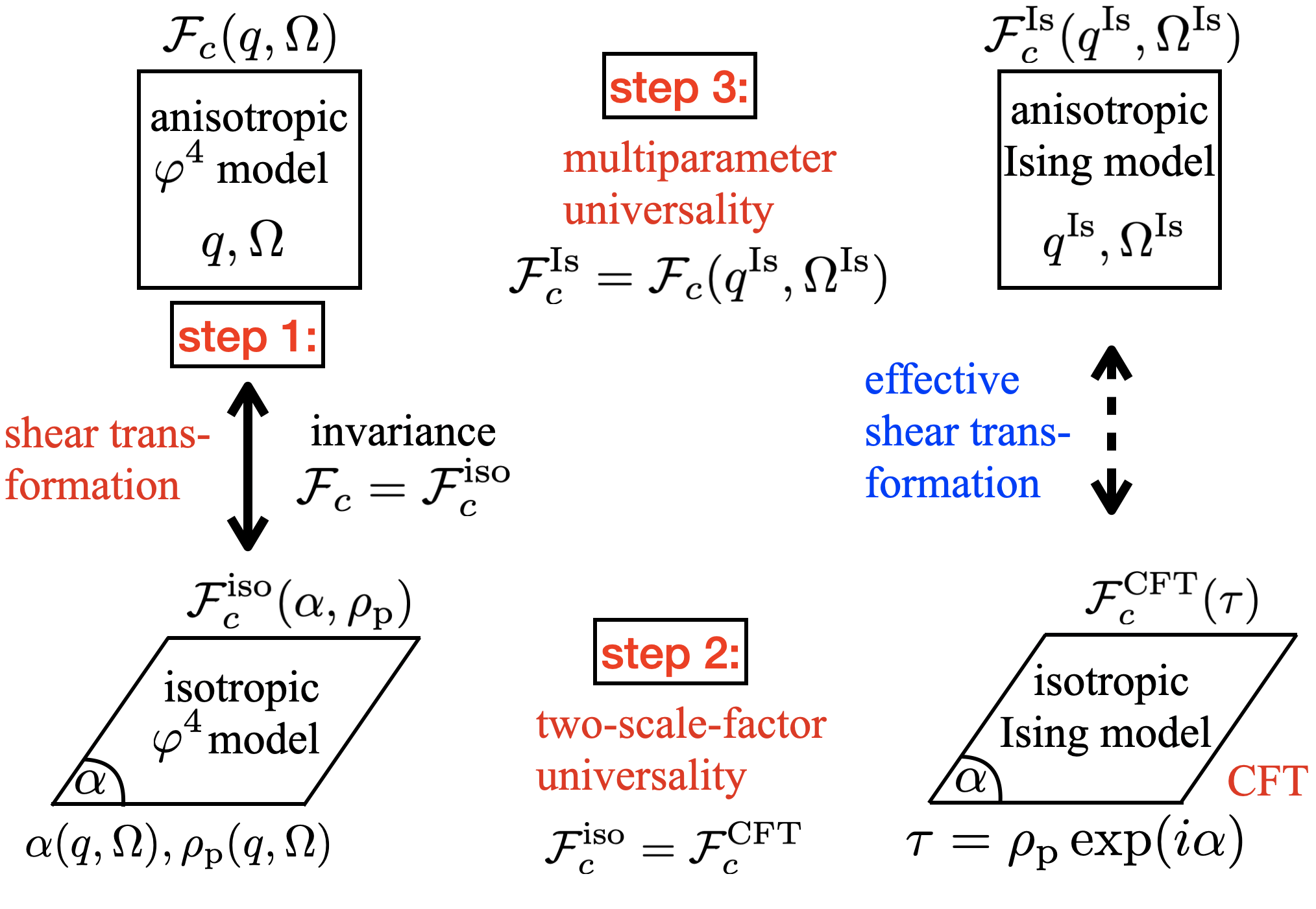
Figure 1: Steps of argumentation for the exact relationships between the critical free energies ${\cal F}_{c}$ of finite anisotropic and isotropic $\varphi^{4}$ and Ising models in $d=2$ (see also Fig. 2).

${\it Step}$ 1: We first consider the anisotropic scalar $\varphi^{4}$ lattice model in a $L_{\parallel}\times L$ rectangle on a square lattice with lattice spacing $\tilde{a}$ and PBC. The Hamiltonian and the total free energy divided by $k_{B}T$ on $N=L_{\parallel}L/\tilde{a}^{2}$ lattice points ${\bf x}_{i}\equiv(x_{i1},x_{i2})$ are defined by dohm2006 ; dohm2008

$$H\! = \!\tilde{a}^{2}\Big{[}\sum_{i}\left(\frac{r_{0}}{2}\varphi_{i}^{2}+u_{0}\varphi_{i}^{4}\right)+\sum_{i,j}\!\!\frac{K_{i,j}}{2}(\varphi_{i}-\varphi_{j})^{2}\Big{]}$$

and by ${\cal F}_{\rm{tot}}=-\ln\{\prod_{i=1}^{N}\int_{-\infty}^{\infty}d\varphi_{i}\exp\left(-H\right)\}$. The large-distance anisotropy is described by the symmetric anisotropy matrix ${\bf A}=({\bf A}_{\alpha\beta})=\left(\begin{array}[]{ccc}a&c\\ c&b\\ \end{array}\right)$,

$${\bf A}_{\alpha\beta} = \lim_{N\to\infty}N^{-1}\sum_{i,j}(x_{i\alpha}-x_{j\alpha})(x_{i\beta}-x_{j\beta})K_{i,j}.\;\;\;\;$$ (4)

Weak anisotropy requires positive eigenvalues $\lambda_{1}>0,\lambda_{2}>0$ of ${\bf A}$, i.e., $\det{\bf A}>0$  footnote . It is known  cd2004 ; dohm2006 ; dohm2008 ; kastening-dohm ; dohm2018 ; dohm2019 ; chen-zhang that anisotropy effects near $T_{c}$ are described by the reduced anisotropy matrix ${\bf\bar{A}}={\bf A}/(\det{\bf A})^{1/d}$ which for $d=2$ has the form dohm2019

$${\bf\bar{A}}(q,\Omega)=\left(\begin{array}[]{ccc}q\;c_{\Omega}^{2}+q^{-1}s_{\Omega}^{2}&\;\;\;(q-q^{-1})\;c_{\Omega}\;s_{\Omega}\\ (q-q^{-1})\;c_{\Omega}\;s_{\Omega}&q\;s_{\Omega}^{2}+q^{-1}\;c_{\Omega}^{2}\end{array}\right)$$ (7)

with $q=(\lambda_{1}/\lambda_{2})^{1/2}=\xi_{0\pm}^{(1)}/\xi_{0\pm}^{(2)}$ and the abbreviations $c_{\Omega}\equiv\cos\Omega,s_{\Omega}\equiv\sin\Omega$ where $\Omega$ determines the principal axes described by the eigenvectors ${\bf e}^{(1)}=(c_{\Omega},s_{\Omega})^{\intercal}$, ${\bf e}^{(2)}=(-s_{\Omega},c_{\Omega})^{\intercal}$ of ${\bf A}$. The exact dependence of $\Omega$ and $q$ on the couplings $K_{i,j}$ through $a,b,c$ has been derived in dohm2019 .

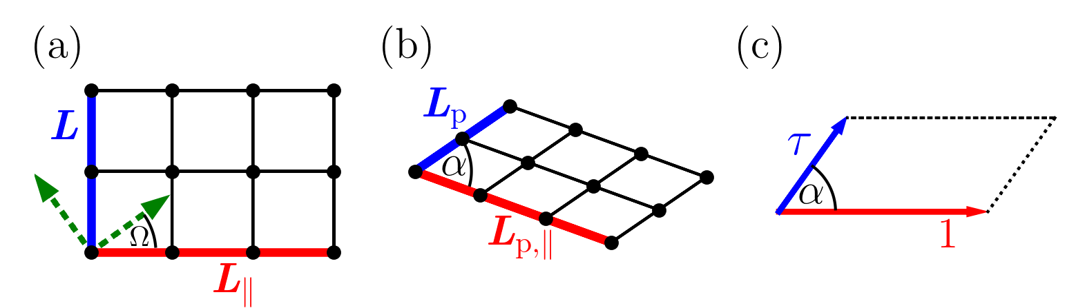
Figure 2: (a) Square lattice with vertical (horizontal) side $\bm{L}$ ($\bm{L}_{\parallel}$) and aspect ratio $\rho=|\bm{L}|/|\bm{L}_{\parallel}|$. Arrows represent the unit vectors ${\bf e}^{(1)},{\bf e}^{(2)}$ of the principal axes for $\Omega=\pi/5$. (b) Transformed lattice for $q=1/2$ with sides $\bm{L}_{\rm{p}}$, $\bm{L}_{\rm{p}\parallel}$, and the angle $\alpha$ and aspect ratio $\rho_{\rm{p}}=|\bm{L}_{\rm{p}}|/|\bm{L}_{\rm{p}\parallel}|$. (c) Parallelogram parametrized by the complex modular parameter $\tau$, (17).

A shear transformation can be performed such that the transformed $\varphi^{4}$ model on a parallelogram (Fig. 2) has changed second moments ${\bf A}^{\prime}_{\alpha\beta}=\delta_{\alpha\beta}$ representing an isotropic system cd2004 ; dohm2008 ; dohm2019 ; kim1987 . The transformations $\bm{L}_{\rm{p}}={\bm{\lambda}}^{-1/2}{\bf U}{\bm{L}}$ and $\bm{L}_{\rm{p}\parallel}={\bm{\lambda}}^{-1/2}{\bf U}{\bm{L}}_{\parallel}$ of the vertical and horizontal sides $\bm{L}=L{\bf e}_{v}$ and $\bm{L}_{\parallel}=L_{\parallel}{\bf e}_{h}$ yield the corresponding transformed sides $\bm{L}_{\rm{p}}$ and $\bm{L}_{\rm{p}\parallel}$ of the parallelogram where the rotation and rescaling matrices

$${\bf{U}}=\left(\begin{array}[]{ccc}\cos\;\Omega&\sin\;\Omega\\ -\sin\;\Omega&\cos\;\Omega\\ \end{array}\right),\;\;\;\;{{\bm{\lambda}}}=\left(\begin{array}[]{ccc}\lambda_{1}&0\\ 0&\;\lambda_{2}\\ \end{array}\right)\;\;\;\;\;\;\;$$ (12)

are employed. The parallelogram is characterized by the angle $0<\alpha<\pi$ between $\bm{L}_{\rm{p}}$ and $\bm{L}_{\rm{p}\parallel}$ and the transformed aspect ratio $\rho_{\rm{p}}=|\bm{L}_{\rm{p}}|/|\bm{L}_{\rm{p}\parallel}|$. We find

$$\cot\alpha(q,\Omega)=-{{\bf\bar{A}}(q,\Omega)}_{12}=(q^{-1}-q)\cos\Omega\;\sin\Omega,\;\;\;\;\;\;\;\;$$ (13)

$$[\rho_{\rm{p}}(\rho,q,\Omega)]^{2}=\rho^{2}\;\frac{{\bf\bar{A}}(q,\Omega)_{11}}{{\bf\bar{A}}(q,\Omega)_{22}}=\rho^{2}\;\frac{\tan^{2}\Omega+q^{2}}{1+q^{2}\tan^{2}\Omega},\;\;\;\;\;\;\;$$ (14)

for arbitrary $\rho,q,\Omega$ which is valid for arbitrary BC. The singular part ${\cal F}^{\rm{iso}}_{c\rm{}}(\alpha,\rho_{\rm{p}})$ of the total free energy at $T_{c}$ of the isotropic parallelogram is a function of $\alpha$ and $\rho_{\rm{p}}$. The shear transformation leaves both the Hamiltonian and the singular part ${\cal F}_{c}$ of the total free energy ${\cal F}_{\rm{tot}}$ at $T_{c}$ invariant dohm2006 ; dohm2008 , thus ${\cal F}_{c}$ is determined by

$${\cal F}_{c}(\rho,q,\Omega)={\cal F}^{\rm{iso}}_{c}\big{(}\alpha(q,\Omega),\rho_{\rm{p}}(\rho,q,\Omega)\big{)}=\rho^{-1}F_{c}(\rho,q,\Omega).$$ (15)

In the strip limit the shear transformation yields  suppl

$$\lim_{\rho\to 0}X_{c}(\rho,q,\Omega)=(q\cos^{2}\Omega+q^{-1}\sin^{2}\Omega)^{-1}X^{\rm{iso}}_{c,\rm{strip}},$$ (16)

where $X^{\rm{iso}}_{c,\rm{strip}}$ is the amplitude on an isotropic strip. Eqs. (15) and (16) demonstrate that ${\cal F}_{c}$, $F_{c}$,and $X_{c}$ depend on microscopic details via $q(a,b,c)$ and $\Omega(a,b,c)$, thus violating two-scale-factor universality. So far it is unknown how to calculate the dependence of ${\cal F}^{\rm{iso}}_{c}$ on $\alpha$ and $\rho_{\rm{p}}$.

${\it Step}$ 2: At this point we invoke two-scale-factor universality for isotropic systems pri ; dohm2018 which means that isotropic $\varphi^{4}$ and Ising models have the same singular parts ${\cal F}^{\rm{iso}}_{c\rm{}}$ and ${\cal F}^{\rm{Is},iso}_{c\rm{}}$. For the Ising model exact information is available from CFT franc1987 ; franc1997 . Via an isotropic continuum description in terms of a free fermion field an exact contribution $Z^{\rm{CFT}}(\tau)$ to the partition function of the $d=2$ isotropic Ising model on a torus at $T_{c}$ has been derived. We choose the same parameters $\alpha$ and $\rho_{\rm{p}}$ as for the isotropic $\varphi^{4}$ model. The Ising parallelogram is described by a complex torus modular parameter franc1997

$$\tau(\alpha,\rho_{\rm{p}})=\mbox{Re}\;\tau+i\;\mbox{Im}\;\tau=\rho_{\rm{p}}\exp(i\;\alpha)$$ (17)

where $\alpha$ is the angle shown in Fig. 2(c) and $\rho_{\rm{p}}=|\tau|$ is the aspect ratio of the Ising parallelogram. The partition function is expressed in terms of Jacobi theta functions $\theta_{i}(0|\tau)\equiv\theta_{i}(\tau)$ (in the notation of franc1997 , see suppl ) as franc1987

$$Z^{\rm{CFT}}(\tau)=\big{(}{|\theta_{2}(\tau)|+|\theta_{3}(\tau)|+|\theta_{4}(\tau)|}\big{)}/\big{(}{2|\eta(\tau)|}\big{)},$$ (18)

with $\eta(\tau)=(\frac{1}{2}\theta_{2}(\tau)\theta_{3}(\tau)\theta_{4}(\tau))^{1/3}$, from which we obtain ${\cal F}^{\rm{CFT}}_{c}(\tau)=\!-\ln Z^{\rm{CFT}}(\tau).$ The singular part of the total free energy of the isotropic Ising model at $T_{c}$ is

$${\cal F}^{\rm{Is},iso}_{c\rm{}}\!\big{(}\tau(\alpha,\rho_{\rm{p}})\big{)}\!={\cal F}^{\rm{CFT}}_{c}\!\big{(}\tau(\alpha,\rho_{\rm{p}})\big{)}\!={\cal F}^{\rm{iso}}_{c\rm{}}\!\big{(}\alpha,\rho_{\rm{p}}\big{)},$$ (19)

where, owing to two-scale-factor universality, the last equation applies to the transformed $\varphi^{4}$ model on the parallelogram. We define $\tau(\rho,q,\Omega)=\tau\big{(}\alpha(q,\Omega),\rho_{\rm{p}}(\rho,q,\Omega)\big{)}$ with $\alpha(q,\Omega)$ and $\rho_{\rm{p}}(\rho,q,\Omega)$ given by (13) and (14). Then we obtain from (19), (15), (1), and (3) our exact result for the Casimir amplitude $X_{c}$ of the anisotropic $\varphi^{4}$ model as

$$X_{c}(\rho,q,\Omega) = -\rho^{2}\;\partial{\cal F}_{c}(\rho,q,\Omega)/\partial\rho$$ (20)

with ${\cal F}_{c}(\rho,q,\Omega)={\cal F}_{c}^{\rm{CFT}}\big{(}\tau(\rho,q,\Omega)\big{)}$ where the nonuniversal expressions for $q(a,b,c)$ and $\Omega(a,b,c)$ dohm2019 have to be inserted. In the strip limit we obtain  suppl

$$X_{c}(0,q,\Omega)=-\pi/[12(q\cos^{2}\Omega+q^{-1}\sin^{2}\Omega)],$$ (21)

in accord with the CFT result $-\pi/12$  bloete ; affleck for $q=1$.

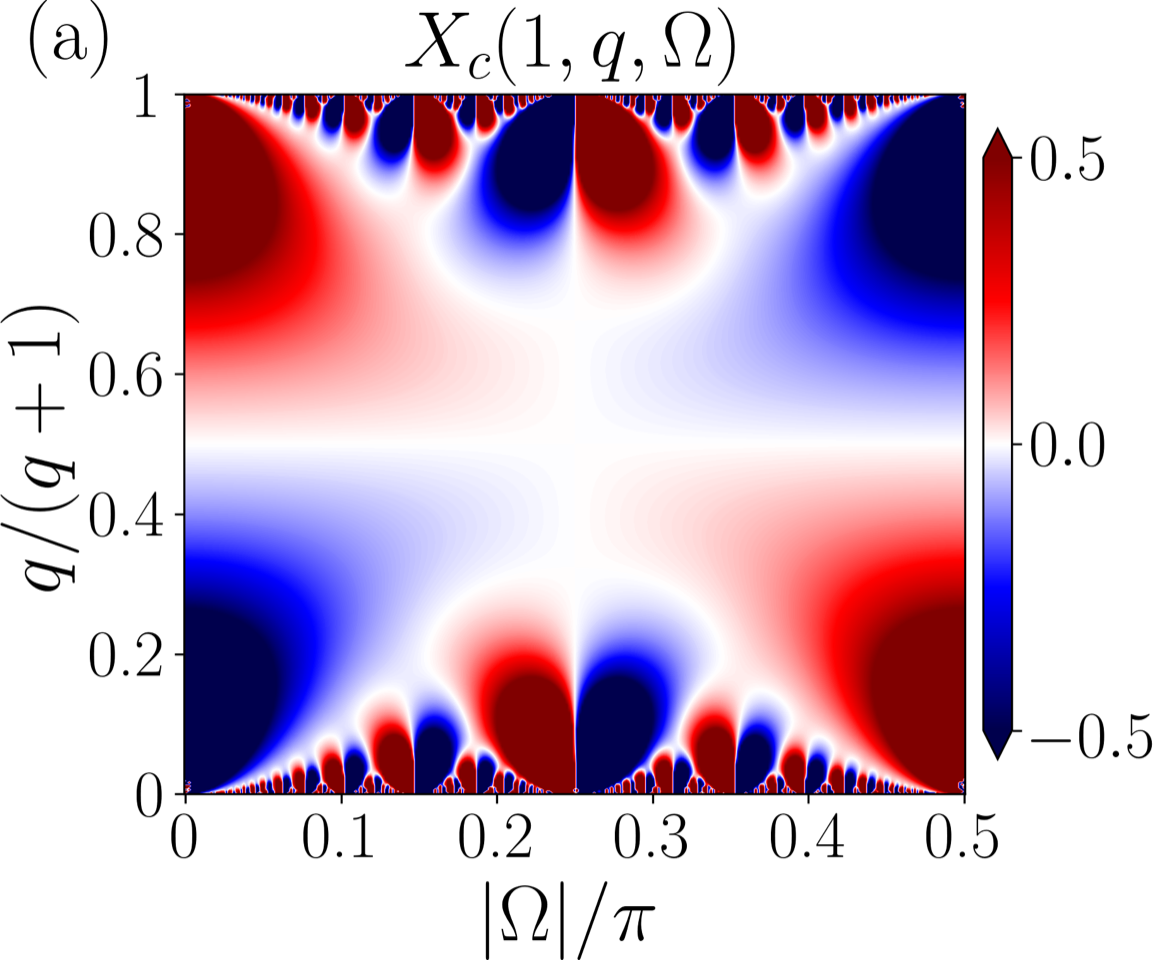
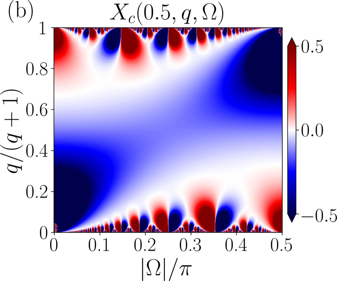
Figure 3: Universal contour plot of the critical Casimir amplitude $X_{c}$ of the anisotropic $d=2$ $\varphi^{4}$ model from (20) for $\rho=1$ in (a) and for $\rho=0.5$ in (b). For the anisotropic $d=2$ Ising model, (22) yields the same plots if $q\to q^{\mathrm{Is}},\Omega\to\Omega^{\mathrm{Is}}$.

In Fig. 3 we present contour plots of $X_{c}$ in the complete $\Omega-q$ plane for $\rho=1$ and $\rho=0.5$. Contrary to the simple ($\Omega,q$) dependence (21) in strip geometry and to the claim that the effects of weak anisotropy are fairly harmless diehl2010 , we find unexpectedly complex structures exhibiting the feature of self-similarity in the regions $q\ll 1$ and $q\gg 1$ near the border lines $q=0$ and $q=\infty$, where $\det{\bf A}=0$ or $\lambda_{\alpha}=0$, i.e., where weak anisotropy breaks down footnote . This self-similarity can be traced back to the property of modular invariance franc1997 $Z^{\rm{CFT}}(\tau)=Z^{\rm{CFT}}(\tau+1)$, $Z^{\rm{CFT}}(\tau)=Z^{\rm{CFT}}(-1/\tau)$ for the partition function of the isotropic Ising model at $T_{c}$ in a parallelogram geometry with PBC, i.e., on a torus, which implies ${\cal F}^{\rm{Is},iso}_{c\rm{}}(\tau)={\cal F}^{\rm{Is},iso}_{c\rm{}}(-1/\tau)={\cal F}^{\rm{Is},iso}_{c\rm{}}(\tau+1).$ This is illustrated by the periodic structure of ${\cal F}^{\rm{Is},iso}_{c\rm{}}$ in the complex $\tau$ plane [Fig. 4(a)] which generates a self-similar structure in the $(\rho_{\rm{p}},\alpha)$ plane [Fig. 4(b)]. The modular transformation $\tau\to-1/\tau$ corresponds to $\rho_{\rm{p}}\to 1/\rho_{\rm{p}},\alpha\to\pi-\alpha$ which yields equivalent parallelograms. The Dehn twist franc1997 $\tau\to\tau+1$ yields parallelograms with different $\rho_{\rm{p}}$ and $\alpha$, but the invariance of ${\cal F}^{\rm{Is},iso}_{c\rm{}}$ can be understood geometrically since a given torus can be cut in different ways such that different parallelograms with PBC are generated which all have the same critical free energy on the same torus. By two-scale-factor universality, the same result applies to ${\cal F}^{\rm{\rm{iso}}}_{c\rm{}}$ of the isotropic $\varphi^{4}$ model on the same torus. The dependence on ($\rho_{\rm{p}},\alpha$) for the isotropic system in Figs. 2(b) and 4(b) is transferred by the shear transformation (13), (14) and by (20) to a corresponding dependence of $X_{c}(\rho,q,\Omega)$ on $(q,\Omega)$ as is shown in Fig. 3. We note that so far no assumption has been made other than the validity of two-scale-factor universality for isotropic systems.

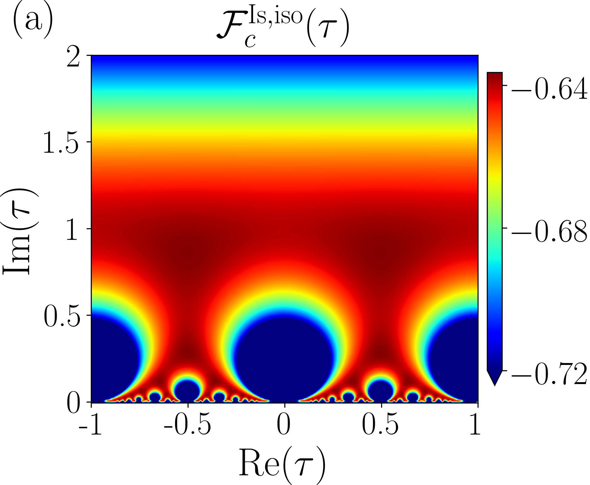
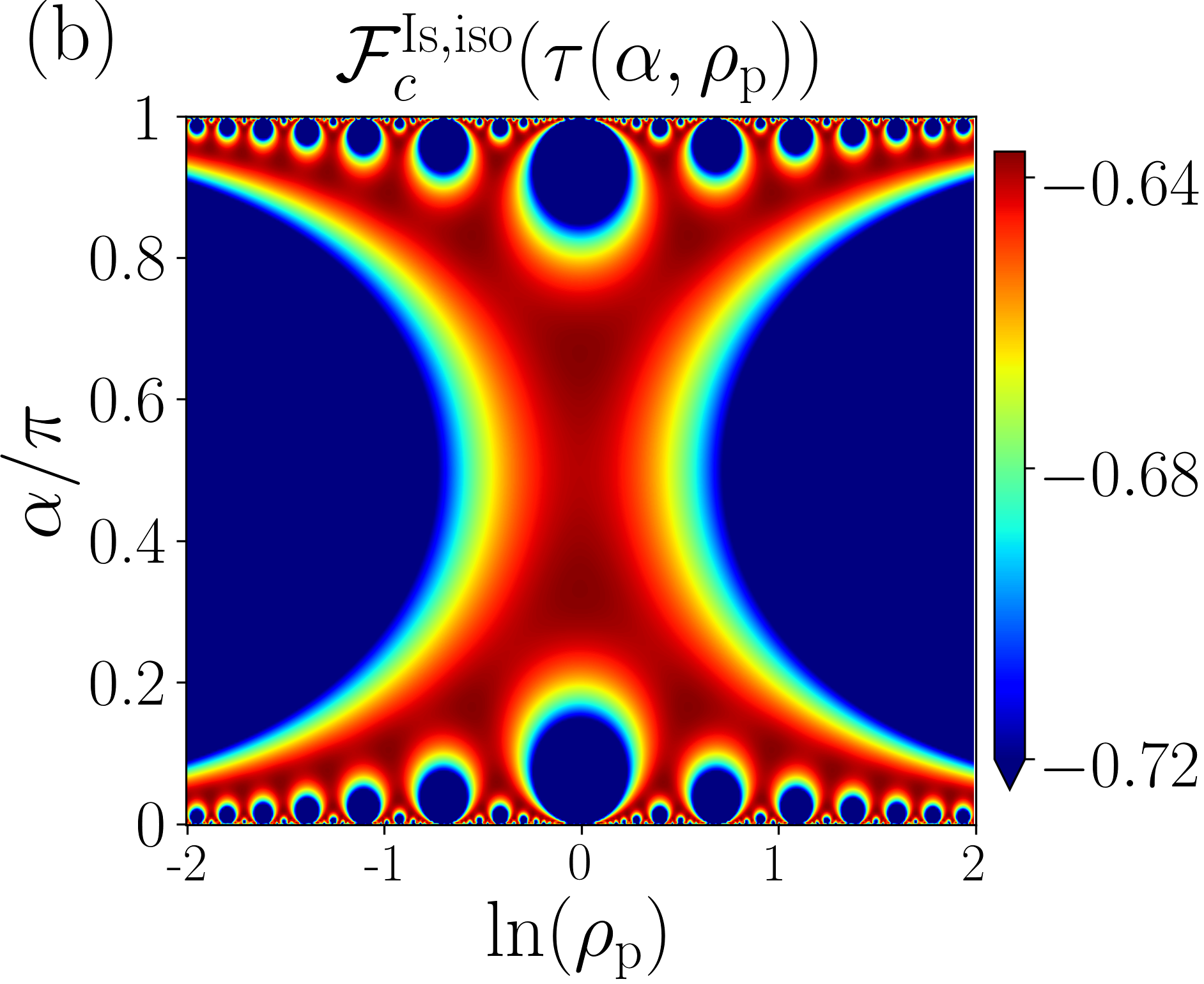
Figure 4: Critical amplitude ${\cal F}^{\rm{Is},iso}_{c\rm{}}$, (19), of the isotropic Ising model in parallelogram geometry (a) in the complex $\tau$ plane and (b) in the $\rho_{p}-\alpha$ plane. The same plot (b) holds for ${\cal F}^{\rm{iso}}_{c\rm{}}$, (19), of the transformed isotropic $\varphi^{4}$ model.

${\it Step}$ 3: We proceed to the anisotropic triangular Ising model on an $L_{\parallel}\times L$ rectangle with the Hamiltonian  dohm2019 ; Indekeu $H^{{\text{\rm{Is}}}}\!=\!-\!\!\sum_{j,k}\big{[}E_{1}\sigma_{j,k}\sigma_{j,k+1}+E_{2}\sigma_{j,k}\sigma_{j+1,k}+E_{3}\sigma_{j,k}\sigma_{j+1,k+1}\big{]}$ with spin variables $\sigma_{j,k}=\pm 1$ on a square lattice with PBC. Both the angle $\Omega^{\rm{Is}}(E_{1},E_{2},E_{3})$ of the principal axes and the ratio of the principal correlation lengths $q^{\rm{Is}}(E_{1},E_{2},E_{3})=\xi_{0\pm}^{(1)\rm{Is}}/\xi_{0\pm}^{(2)\rm{Is}}$ are known functions of $E_{1},E_{2},E_{3}$ dohm2019 . Multiparameter universality was proven for bulk systems in dohm2019 , thus the exact critical bulk correlation function is governed by the Ising anisotropy matrix ${\bf\bar{A}}^{\rm{Is}}={\bf\bar{A}}(q^{\rm{Is}},\Omega^{\rm{Is}})$ with the same matrix ${\bf\bar{A}}$ as in (7) for the $\varphi^{4}$ model, but with $q$ and $\Omega$ replaced by $q^{\rm{Is}}$ and $\Omega^{\rm{Is}}$. Since bulk and finite-size properties are governed by the same anisotropy matrix dohm2018 we predict that the exact critical Casimir amplitude of the anisotropic Ising model is given by

$$X^{\rm{Is}}_{c}(\rho,q^{\rm{Is}},\Omega^{\rm{Is}})=-\rho^{2}\;\partial{\cal F}_{c}(\rho,q^{\rm{Is}},\Omega^{\rm{Is}})/\partial\rho,$$ (22)

where ${\cal F}_{c}(\rho,q^{\rm{Is}},\Omega^{\rm{Is}})$ is the same function as in (20) but now the results for $q^{\rm{Is}}(E_{1},E_{2},E_{3})$ and $\Omega^{\rm{Is}}(E_{1},E_{2},E_{3})$ of the Ising model dohm2019 have to be inserted. Our predictions go far beyond all previous special results bloete ; affleck ; rud2010 ; FF ; salas ; izmail ; kastening2012 ; HH2019 for confined isotropic and anisotropic Ising models. Here we have succeeded in treating the general anisotropic case of an arbitrary direction of the principal axes described by a nonzero angle $\Omega^{\rm{Is}}$ in a finite geometry with an arbitrary aspect ratio $\rho$. This is of physical relevance for general anisotropic systems with more complicated interactions whose principal axes generically have skew directions relative to the symmetry axes of the underlying lattice. This advance is made possible by our new approach of combining exact relations of anisotropic $\varphi^{4}$ lattice theory with exact results of CFT. Specifically our predictions agree with Ising-model results for isotropic strips bloete ; affleck ; rud2010 , rectangles FF , and parallelograms salas as well as for anisotropic strips kastening2012 and rectangles izmail ; HH2019 which constitutes a direct confirmation of multiparameter universality for confined systems. Thus we predict that the results in Fig. 3 for the $\varphi^{4}$ model are valid also for the Ising model after substituting $q\to q^{\mathrm{Is}},\Omega\to\Omega^{\mathrm{Is}}$, i.e., the $(q,\Omega)$ representation has a universal character that is applicable to all weakly anisotropic systems in the ($d=2,n=1$) universality class. It becomes nonuniversal if the dependence of $(q,\Omega)$ and $(q^{\rm{Is}},\Omega^{\rm{Is}})$ on $a,b,c$ and $E_{1},E_{2}$, $E_{3}$ is inserted. We denote these Casimir amplitudes by $X_{c}[\rho,a/c,b/c]$ and $X^{\rm{Is}}_{c}[\rho,E_{1}/E_{3},E_{2}/E_{3}]$. They are shown in Fig. 5 for $\rho=1$. The nonuniversal differences between $X_{c}$ and $X^{\rm{Is}}_{c}$ confirm the prediction cd2004 ; dohm2006 ; dohm2008 ; dohm2018 that the Casimir amplitude $X_{c}$ for weakly anisotropic systems is not a universal quantity. Even if it is known for one anisotropic system it cannot be predicted for other anisotropic systems of the same universality class since $\Omega$ generically depends in an unknown nonuniversal way on the anisotropic interactions dohm2019 .

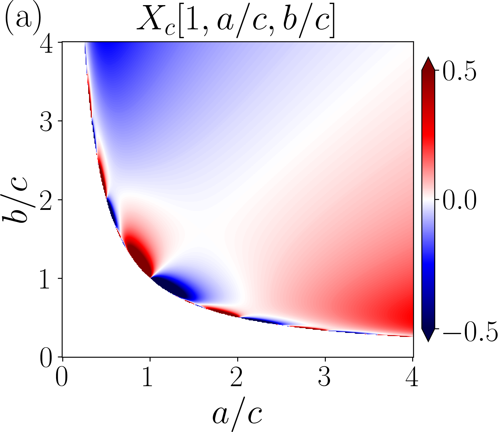
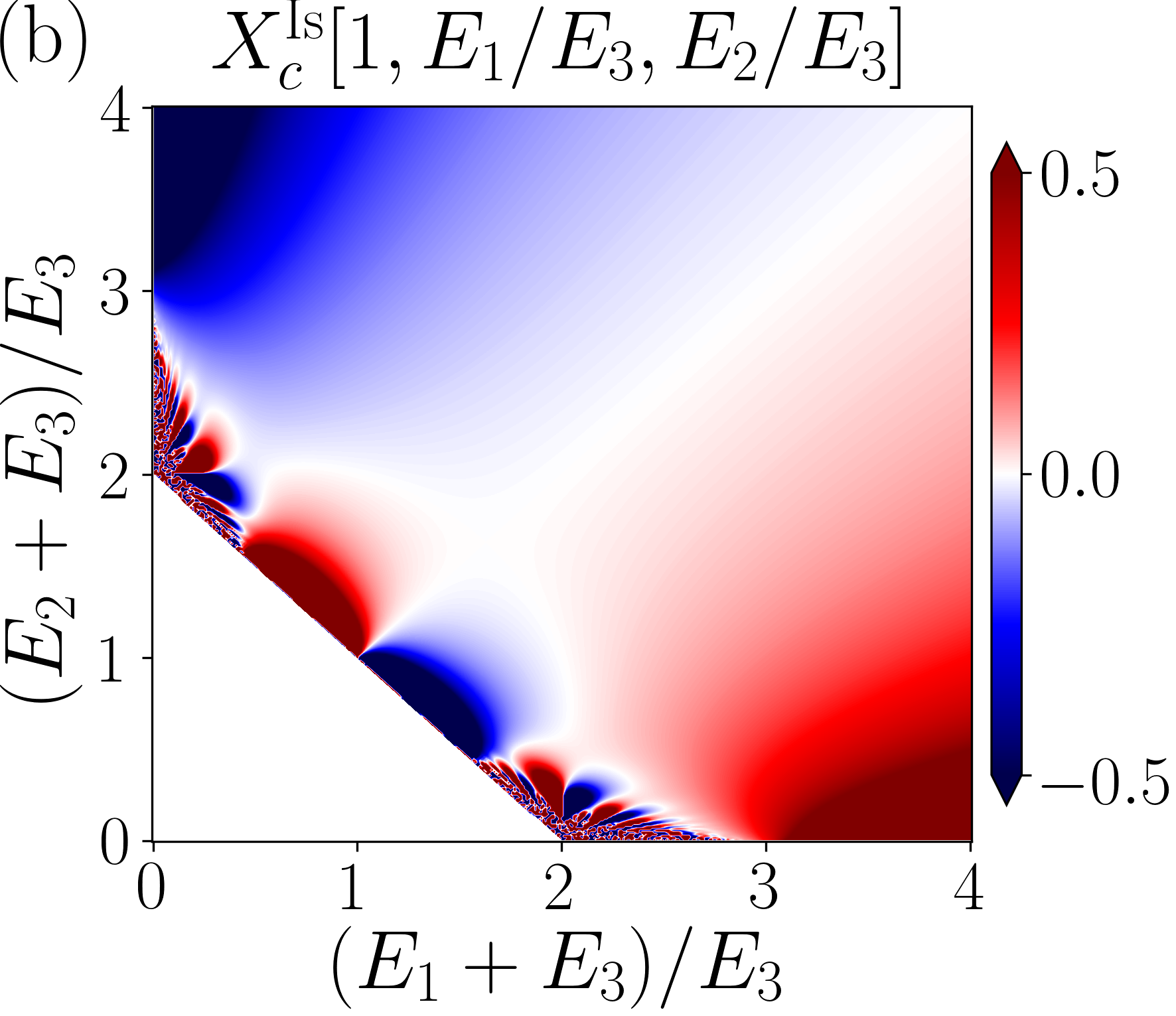
Figure 5: Nonuniversal critical Casimir amplitudes $X_{c}$ and $X^{\rm{Is}}_{c}$ for $\rho=1$ of the $d=2$ $\varphi^{4}$ and Ising models for (a) $\det{\bf A}=ab-c^{2}>0$, (b) $E_{1}+E_{2}>0,E_{1}+E_{3}>0,E_{2}+E_{3}>0$ Berker .

Figure 6: Universal contour plots of critical and low-temperature Casimir amplitudes of the $d=3$ $\varphi^{4}$ theory for $n=\infty$ dohm2018 ; suppl with planar anisotropies (28): $\hat{X}_{c}$ for $\rho=1$ with ${\bf\bar{A}^{(x,y)}_{3}}$ in (a) and $\hat{X}_{0}$ for $\rho=0.5$ with ${\bf\bar{A}^{(y,z)}_{3}}$ in (b).

In the following we demonstrate that self-similar structures exist more generally for $O(n)$-symmetric systems with PBC for $d=3,n\geq 1$ with a $3\times 3$ anisotropy matrix ${\bf A_{3}}$. Consider a $L_{\parallel}^{2}\times L$ geometry with $\rho=L/L_{\parallel}$. In dohm2018 the scaling function $X(\hat{x},\rho,{\bf\bar{A}_{3}})$ of the Casimir force of the $\varphi^{4}$ model has been derived for $n\geq 1$, where $\hat{x}\propto(T-T_{c})L^{1/\nu}$ is the scaling variable. This includes the low-temperature amplitude $X_{0}(\rho,{\bf\bar{A}_{3}})\equiv X(-\infty,\rho,{\bf\bar{A}_{3}})$ due to the Goldstone modes for $n\geq 2$. In particular, the exact result $\hat{X}=\lim_{n\to\infty}\;X/n$ has been derived in the large-$n$ limit. At fixed $\hat{x}$ the anisotropy effect is completely contained in the function

$$K_{3}(y,{\bf\widehat{C}})=\sum_{\bf m}\;\exp(-y\;{\bf m}\cdot{\bf\widehat{C}m})$$ (23)

where $y$ is independent of ${\bf\bar{A}_{3}}$. The sum $\sum_{\bf m}$ runs over ${\bf m}=(m_{1},m_{2},m_{3})\;,m_{\alpha}=0,\pm 1,...,\pm\infty$ and the $3\times 3$ matrix ${\bf\widehat{C}}$ has the elements $\widehat{C}_{\alpha\beta}=\rho_{\alpha}\;\rho_{\beta}\;({\bf\bar{A}_{3}})_{\alpha\beta}$ with $\rho_{1}=\rho_{2}=\rho,\rho_{3}=1$. We consider two types of planar anisotropies as described by the anisotropy matrices

$${\bf\bar{A}^{(x,y)}_{3}}=\left(\begin{array}[]{ccc}{\bf\bar{B}_{h}}&0\\ 0&{1}\end{array}\right),\;\;\;{\bf\bar{A}^{(y,z)}_{3}}=\left(\begin{array}[]{ccc}{1}&0\\ 0&{\bf\bar{B}_{v}}\end{array}\right).$$ (28)

In (28) the $2\times 2$ submatrices ${\bf\bar{B}_{h}}$ and ${\bf\bar{B}_{v}}$ describe anisotropies in the “horizontal” $x-y$ and “vertical” $y-z$ planes, respectively. The difference between these cases is that the Casimir force defined in (2) is perpendicular to the $x-y$ anisotropy in case of ${\bf\bar{A}^{(x,y)}_{3}}$ whereas it is parallel to the $y-z$ anisotropy in case of ${\bf\bar{A}^{(y,z)}_{3}}$. Both ${\bf\bar{B}_{h}}$ and ${\bf\bar{B}_{v}}$ have the same form as in (7), with $(q,\Omega)$ replaced by $(q_{\bf\bar{B}},\Omega_{\bf\bar{B}})$. This suggests that self-similar structures exist for $d=3$ like those found for $d=2$. This is indeed verified by evaluating the exact results for $\hat{X}_{c}$ and $\hat{X}_{0}$ of dohm2018 for $d=3,n=\infty$ with the planar anisotropies (28) as shown in Fig. 6. We find similar structures from dohm2018 for any finite $n$ and $\hat{x}$. The self-similar structures of Fig. 6 disappear in the film limit $\rho\to 0$ dohm2018 at finite $L$ but are maintained in the cylinder limit $\rho\to\infty$ dohm2011 at finite $L_{\parallel}$.

We find that, to some extent, this self-similarity can be traced back to the modular invariance of $K_{3}(y,{\bf\widehat{C}})$, (23). Since a symmetric matrix ${\bf\bar{B}}$ with $\det{\bf\bar{B}}=1$ contains only two independent matrix elements, it can be expressed as

$${\bf\bar{B}}=\frac{1}{\mbox{Im}(\tau_{\bf\bar{B}})}\left(\begin{array}[]{ccc}|\tau_{\bf\bar{B}}|^{2}&-\mbox{Re}(\tau_{\bf\bar{B}})\\ -\mbox{Re}(\tau_{\bf\bar{B}})&1\\ \end{array}\right),$$ (31)

where $\tau_{\bf\bar{B}}=\mbox{Re}(\tau_{\bf\bar{B}})+i\;\mbox{Im}(\tau_{\bf\bar{B}})$ is a complex number with $\mbox{Im}(\tau_{\bf\bar{B}})>0$. Based on the one-to-one relation (31) between ${\bf\bar{B}}$ and $\tau_{\bf\bar{B}}$, we can relate a modular transformation $\tau_{\bf\bar{B}}\to\tau_{\bf\bar{B}^{\prime}}$ to a corresponding matrix ${\bf\bar{B}}^{\prime}$, with, e.g., $\tau_{\bf\bar{B}^{\prime}}=\tau_{\bf\bar{B}}+1$ for the Dehn twist. The function $K_{3}$ remains invariant under such transformations for ${\bf\bar{A}_{3}}={\bf\bar{A}^{(y,z)}_{3}}$, $\rho=1$ and for ${\bf\bar{A}_{3}}={\bf\bar{A}^{(x,y)}_{3}}$ and arbitrary $\rho$ suppl . This is parallel to the modular invariance of $Z^{\rm{CFT}}(\tau)$. More generally, we expect self-similar structures also for $d=3$ systems with non-planar anisotropies and PBC.

Conclusion and outlook - We have studied the dependence of finite-size effects on the principal correlation lengths and principal axes for the case of PBC. For $d=2$, we have achieved a breakthrough by identifying unexpected self-similar structures via the combination of isotropic CFT with anisotropic $\varphi^{4}$ theory. For $d=3$, our analysis paves the way towards an exploration of finite-size effects near the borderlines where weak anisotropy breaks down not only near $T_{c}$ but also in the Goldstone-dominated region. On the basis of $d=3$ finite-size theories Esser ; CDS ; dohm2018 ; dohm2008 and owing to multiparameter universality we predict that in all $O(n)$-symmetric systems with weak anisotropies and PBC the self-similar structures described in this Letter appear also in various physical quantities such as the specific heat and susceptibility. Self-similar structures do not appear for simple anisotropies with $\Omega=0,\pi/4$ studied previously izmail ; Selke2009 ; HH2019 ; kim1987 ; Yurishchev although two-scale-factor universality is violated in these cases. Our results provide strong motivation for investigating the case of other boundary conditions and to study finite-size effects in anisotropic systems such as superconductors, magnetic materials, solids with structural phase transitions and near magnetic-field-induced phase transitions lin where the interplay between spatial and spin anisotropy is relevant. In particular, it would be important to explore the crossover from weak anisotropy to strong anisotropy of cooperative phenomena such as those near Lifshitz points.

References

- (1) M. Kardar and R. Golestanian, Rev. Mod. Phys. 71, 1233 (1999).
- (2) M. Krech, The Casimir Effect in Critical Systems (World Scientific, Singapore, 1994).
- (3) A. Gambassi, J. Phys. Conf. Ser. 161, 012037 (2009).
- (4) A. Ajdari, L. Peliti, and J. Prost, Phys. Rev. Lett. 66, 1481 (1991); H. Li and M. Kardar, Phys. Rev. Lett. 67, 3275 (1991); F. Karimi Pour Haddadan, J. Phys.: Conden. Matter 29, 065101 (2017).
- (5) G.A. Williams, Phys. Rev. Lett. 92, 197003 (2004).
- (6) V. Dohm, Phys. Rev. E 84, 021108 (2011).
- (7) V. Privman, A. Aharony, and P.C. Hohenberg, in Phase Transitions and Critical Phenomena, edited by C. Domb and J.L. Lebowitz (Academic, New York, 1991), Vol. 14, p. 1.
- (8) V. Dohm, Phys. Rev. E 97, 062128 (2018).
- (9) V. Dohm, Phys. Rev. E 77, 061128 (2008).
- (10) V. Privman and M.E. Fisher, Phys. Rev. B 30, 322 (1984).
- (11) V. Privman, in Finite Size Scaling and Numerical Simulation of Statistical Systems, edited by V. Privman (World Scientific, Singapore, 1990), p. 1.
- (12) H. W. J. Blöte, J. L. Cardy, and M. P. Nightingale, Phys. Rev. Lett. 56, 742 (1986).
- (13) I. Affleck, Phys. Rev. Lett. 56, 746 (1986).
- (14) J. Dubail, R. Santachiara, and T. Emig, EPL 112, 66004 (2015); J. Stat. Mech. 033201 (2017).
- (15) X.S. Chen and V. Dohm, Phys. Rev. E 70, 056136 (2004).
- (16) V. Dohm, J. Phys. A 39, L 259 (2006).
- (17) B. Kastening and V. Dohm, Phys. Rev. E 81, 061106 (2010).
- (18) V. Dohm, Phys. Rev. Lett. 110, 107207 (2013).
- (19) J. L. Cardy, in Phase Transitions and Critical Phenomena, edited by C. Domb and J. L. Lebowitz (Academic, New York, 1987), Vol. 11, p. 55.
- (20) J. L. Cardy, Nucl. Phys. B 275, 200 (1986).
- (21) J. L. Cardy, Nucl. Phys. B 270, 186 (1986).
- (22) P. Di Francesco, H. Saleur, and J. B. Zuber, Nucl. Phys. B 290, 527 (1987).
- (23) For see C. Itzikson, Nucl. Phys. B (Proc. Suppl.) 1A, 185 (1987).
- (24) J. L. Cardy, in Fields, Strings and Critical Pheneomena, edited by E. Brézin and J. Zinn-Justin (North-Holland Amsterdam, 1990), p.169.
- (25) P. Di Francesco, P. Mathieu, and D. Sénéchal, Conformal Field Theory (Springer-Verlag New York, 1997).
- (26) V. Dohm, Phys. Rev. E 100, 050101(R) (2019).
- (27) V. Dohm, EPL 86, 20001 (2009).
- (28) For , the large-distance behavior is affected by the fourth-order moments of the couplings , as defined in Eq. (8.21) of dohm2008 .
- (29) X.S. Chen and H.Y. Zhang, Int. J. Mod. Phys. B 21, 4212 (2007).
- (30) For an equivalent transformation applied to the eight-vertex and hard hexagon models for the special case in strip geometry with PBC see D. Kim and P.A. Pearce, J. Phys. A 20, L 451 (1987).
- (31) See the Supplemental Material for (i) the derivation of Eqs. (16) and (21) for the critical Casimir force in anisotropic strips, (ii) the notation of the Jacobi theta functions, (iii) the analytic expressions for the systems from Ref. dohm2018 , (iv) the derivation of the modular invariance of .
- (32) M. Burgsmüller, H.W. Diehl, and M.A. Shpot, J. Stat. Mech. P11020 (2010).
- (33) J.O. Indekeu, M.P. Nightingale, and W.V. Wang, Phys. Rev. B 34, 330 (1986).
- (34) J. Rudnick, R. Zandi, A. Shackell, and D. Abraham, Phys. Rev. E 82, 041118 (2010).
- (35) A. E. Ferdinand and M. E. Fisher, Phys. Rev. 185, 832 (1969). This case corresponds to .
- (36) J. Salas, J. Phys. A 35, 1833 (2002). This case corresponds to .
- (37) B. Kastening, Phys. Rev. E 86, 041105 (2012).
- (38) N. Sh. Izmailian, J. Phys. A 45, 494009 (2012).
- (39) H. Hobrecht and A. Hucht, SciPost Phys. 7, 026 (2019).
- (40) R. M. F. Houtappel, Physica 16, 425 (1950).
- (41) A. Esser, V. Dohm, and X.S. Chen, Physica A 222, 355 (1995).
- (42) X.S. Chen, V. Dohm, and N. Schultka, Phys. Rev. Lett. 77, 3641 (1996).
- (43) M.A. Yurishchev, Phys. Rev. B 50, 13533 (1994).
- (44) W. Selke and L.N. Shchur, J. Phys. A 38, L 739 (2005); Phys.Rev. E 80, 042104 (2009).
- (45) S.-Z. Lin, K. Barros, E. Mun, J.-W. Kim, M. Frontzek, S. Barilo, S. V. Shiryaev, V. S. Zapf, and C. D. Batista, Phys. Rev. B 89, 220405(R) (2014).