Non-Convex Optimization with Spectral Radius Regularization

Abstract

We develop a regularization method which finds flat minima during the training of deep neural networks and other machine learning models. These minima generalize better than sharp minima, allowing models to better generalize to real word test data, which may be distributed differently from the training data. Specifically, we propose a method of regularized optimization to reduce the spectral radius of the Hessian of the loss function. Additionally, we derive algorithms to efficiently perform this optimization on neural networks and prove convergence results for these algorithms. Furthermore, we demonstrate that our algorithm works effectively on multiple real world applications in multiple domains including healthcare. In order to show our models generalize well, we introduce different methods of testing generalizability.

1 Introduction

Finding flat minima solutions is important to many optimization problems, especially those found in machine learning applications. Such models generalize better than sharp minima because the value of the objective function remains similar for flat minima if the data is shifted, distorted, or otherwise changed. Thus, in practice, optimal machine learning models with flatter optima should perform better than those with sharper ones on test data that is distributed differently than the original training data.

Here, we define flat minima as those with a small spectral radius (largest absolute eigenvalue) of the Hessian of the objective function and sharp minima as those where the spectral radius is large. For minima where this spectral radius is small, there is no direction away from this point in which the objective function immediately and rapidly increases. Therefore, by regularizing our optimization of models with respect to this spectral radius, we are able to obtain solutions that are less susceptible to errors or biases in the training or test data.

However, this regularization presents certain challenges: For large neural networks, computing and storing the Hessian and the third derivative tensor are infeasible; therefore we need to develop methods to efficiently compute the regularization term and its gradient. We also needed to design methods to introduce errors and biases into the data in order to test the generalizability of these models.

To tackle these challenges, we build a method to regularize the spectral radius while computing Hessian-vector products. We present results with different regularization parameters to show our methodology is stable. We introduce multiple methods to test generalizability, tailored to specific problems. Our contributions include:

• We develop an algorithm for regularizing neural networks with respect to the spectral radius of the Hessian, a novel use of a derivative measure for such regularization.

• We apply and extend differential operators used to efficiently compute Hessian-vector products for neural networks.

• We provide formal proofs on convergence and other properties of our algorithm.

• We present experimental results on multiple real world data sets across different domains, designing specific methods to test generalizability.

In Section 2, we review existing literature related to our research. In Section 3, we derive the algorithm used for our regularization. In Section 4, we discuss convergence results and other properties of the algorithm. In Section 5, we describe different generalizability tests and present results of our experiments with regularization on various data sets.

2 Related Work

Existing works discussed how different learning methods affect the ability of neural networks to converge to flat minima. Keskar et al. [2016] observed that large-batch stochastic gradient descent (SGD) and its variants, such as adaptive moment estimation (Adam), tend to converge to sharp minima, while small-batch methods converge to flat minima. This implies that small-batch methods generalize better than large-batch methods, as the training function at sharp minima is more sensitive. Some possible causes for this include that large-batch methods over-fit, are attracted to saddle points, lack the explorative properties of small-batch methods (tend to converge to the minima close to the initial weights). Yao et al. [2018] showed that large-batch training of neural networks converges to points with larger Hessian spectrum (both in terms of dominant and other eigenvalues) which shows poor robustness. Jastrzebski et al. [2018] extended these claims in showing that a large learning rate also leads to flatter minima that generalize better than sharper minima.

Others suggested different ways to measure and find flat minima, including different objective functions and optimization algorithms. Ma et al. [2019] suggests that Kronecker-Factored Approximate Curvature (K-FAC) [Martens and Grosse, 2015], an approximate second-order method may yield generalization improvements over first-order SGD. Chaudhari et al. [2016] proposed an entropy-based objective function to find solutions in flat regions and an algorithm (called Entropy-SGD) to conduct the optimization. He et al. [2019] observed that at local minima of deep networks, there exist many asymmetric directions where the loss sharply increases, which they call “asymmetric valleys.” They propose weight averaging along the SGD trajectory to bias solutions in favor of the flat side. Chaudhari et al. [2016] also noted that many neural networks, trained on various data sets using SGD or Adam, converge to a point with a large number of near-zero eigenvalues, along with a long positive tail, and shorter negative tail. These observations about the imbalanced eigenspectrum by Chaudhari et al. [2016] and He et al. [2019] are of special interest to us, as our regularization method, which attempts to reduce the spectral radius of the Hessian, should be tailored to avoid these asymmetric valleys.

While Yoshida and Miyato [2017] developed a spectral norm radius regularization method, it looks solely at the spectral radius of a neural network’s weight matrices, rather than the spectral radius of the Hessian of the loss function. While they experimentally show that their regularization method has a small generalization gap (between the training and test set), their method also had higher Hessian spectral radius than vanilla SGD, weight-decay, and adversarial methods. We believe our regularization method and generalization tests more directly address the task of finding flat minima and evaluating their generalizability.

3 Algorithm

	Definition
$w$	weights of neural network
$f(w)$	objective function
$H(w)$	Hessian of $f(w)$
$\rho(w)$	spectral radius of $H(w)$
$\mu$	degree of regularization
$K$	goal of $\rho(w)<K$
$\bar{v}$	eigenvector corresponding to spectral radius
$h(w)$	$f(w)+\mu\max\{0,\rho(w)-K\}$

Table 1: Variable Definitions

For reference, we provide a summary of the main variables used and their corresponding definitions in Table 1. We choose to express our problem as a regularized optimization problem, rather than a constrained optimization or min-max problem. Thus, our optimization problem is:

$$\min\limits_{w}f(w)+\mu\max\{0,\rho(w)-K\},$$

where weights $w\in\mathbb{R}^{n}$, $f(w)$ is a non-convex objective function, $\rho(w)$ is the spectral radius of the Hessian $H(w)$ of $f(w)$ (i.e., the maximal absolute eigenvalue), and $\mu,K$ are regularization parameters. For convenience, we denote $h(w):=f(w)+\mu\max\{0,\rho(w)-K\}$.

The caveat is: we cannot directly compute $H(w)$. For large neural networks of size $\mathcal{O}(n)$, computing and storing objects of size $\mathcal{O}(n^{2})$ (such as the Hessian) is infeasible. However, we can efficiently compute the Hessian-vector product $H(w)v$ for a given $v\in\mathbb{R}^{n}$ using methods discussed in Section 3.1.1.

Our goal is to design efficient algorithms for solving this minimization problem. In Section 3.1, we discuss how to compute the regularized term and its gradient. In Section 3.2, we present and explain different variants of our algorithm.

3.1 Gradients of Regularization Term

The spectral radius can be expressed $\rho(w)=\bar{v}^{T}H(w)\bar{v}$, where $\bar{v}$ is the eigenvector corresponding with the maximum absolute eigenvalue. In order to compute gradient update steps, we need to calculate $\nabla\rho$.

Lemma 3.1.

For distinct eigenvalues of symmetric matrix $A(x):\mathbb{R}\to\mathbb{R}^{n\times n}$,

$$\frac{d\lambda_{k}(x)}{dx}=v_{k}^{T}\frac{dA(x)}{dx}v_{k},$$

where $v_{k}$ is the eigenvector corresponding to eigenvalue $\lambda_{k}$.

Aa, van der et al. [2007] proves Lemma 3.1. The expression for this derivative is more complicated with repeating eigenvalues, so we assume that the eigenvalue in question is distinct (in practice, this is almost surely the case).

Using this result and assumption, we express $\nabla\rho(w)=\bar{v}^{T}\nabla H(w)\bar{v}$. Thus, if we can efficiently compute $H(w)v$ and $v^{T}\nabla H(w)v$ for $w,v\in\mathbb{R}^{n}$, we can respectively calculate $\rho(w)$ and $\nabla\rho(w)$.

3.1.1 Hessian-Vector Operations

In order to compute $H(w)v$ and $v^{T}\nabla H(w)v$ for large neural networks with $w,v\in\mathbb{R}^{n}$, we extend Pearlmutter94fastexact operator. We define this differential operator:

Definition 3.1.

$\mathcal{R}\left\{f(w);v\right\}:=\left.\frac{\partial}{\partial r}f(w+rv)\right|_{r=0}$.

Note that $\mathcal{R}\left\{\nabla f(w);v\right\}=H(w)v$. Thus, by applying the differential operator $\mathcal{R}\left\{\cdot\right\}$ to the forward and backwards passes used to calculate the gradient, we can compute $\rho(w)$ efficiently.

We extend this to $\mathcal{R}^{2}\left\{\cdot\right\}$ by computing $\mathcal{R}^{2}\left\{x\right\}$ and $\mathcal{R}^{2}\left\{y\right\}$ during the forward pass and $\mathcal{R}^{2}\left\{\nabla_{y}h\right\}$, $\mathcal{R}^{2}\left\{\nabla_{x}h\right\}$, and $\mathcal{R}^{2}\left\{\nabla_{w}h\right\}$ during the backward pass. Our formulas and the derivation can be found in Appendix A. Since $\mathcal{R}^{2}\left\{\nabla f(w);v\right\}=v^{T}\nabla H(w)v$, this allows us to efficiently compute $\nabla\rho(w)$.

These methods keep the number of stored values $\mathcal{O}(n)$, while directly computing the Hessian and third-derivative tensor would require $\mathcal{O}(n^{2})$ and $\mathcal{O}(n^{3})$ storage (which for large networks is infeasible).

3.2 Algorithms

Here, we present two versions of our algorithm: an exact gradient descent algorithm (Algorithm 1) and a batch stochastic gradient descent algorithm (Algorithm 2). The first is ideal, but impractical; hence, we need a more practical stochastic algorithm. Here, for simplicity, we hide the $w_{k}$ dependencies (where $w_{k}$ is the value of weights $w$ at iteration $k$) for many of the variables by defining: $f_{k}:=f(w_{k})$, $\rho_{k}:=\rho(w_{k})$, $\nabla f_{k}:=\nabla f(w_{k})$, etc. Step size $\alpha_{k}$ is some predefined function of iteration $k$.

We start with Algorithm 1, a gradient descent algorithm with exact values for the eigenvectors and spectral radius. In practice, these values are often difficult to compute exactly due to computational and storage constraints. For our stochastic algorithm, we relax this exact constraint and compute or approximate values based on a batch (rather than the full data set). We examine the convergence properties of Algorithm 1 in Section 4.1.

1 Initialize $w_{0}$. Set $k=0$.

2 while convergence criteria not met do

3       Compute $f_{k}$ and $\nabla f_{k}$

4       Compute $\rho_{k}$ and $\bar{v}_{k}$

5       Compute $\nabla\rho_{k}$

6       Update $h_{k}$ and $\nabla h_{k}$

7       Set $w_{k+1}=w_{k}-\alpha_{k}h_{k}$

8       $k++$

Algorithm 1 Gradient Descent

Building off the exact gradient descent algorithm, we develop a more practical stochastic algorithm. Algorithm 2, uses batch stochastic gradient descent (rather than gradient descent) and power iteration to compute the eigenvector (rather than an exact method). Due to the implementation of $\mathcal{R}\left\{\cdot\right\}$ and $\mathcal{R}^{2}\left\{\cdot\right\}$, the storage requirements $\mathcal{O}(n)$ are not extensive. Also, since the Hessian is symmetric, the power iteration converges at a rate proportional to the square of the ratio between the two largest eigenvalues $\mathcal{O}\left(|\lambda_{1}/\lambda_{2}|^{2}\right)$, instead of the typical linear rate $\mathcal{O}\left(|\lambda_{1}/\lambda_{2}|\right)$. The convergence properties of Algorithm 2 are studied in Section 4.2.

1 Initialize $w_{0}$. Set $k=0$.

2 while convergence criteria not met do

3       for each batch $B$ do

4             Compute $\nabla f_{k}=\frac{1}{|B|}\sum\limits_{i\in B}\nabla f_{k}$

             /* Power iteration */

5             while $||u-\lambda v||>\varepsilon$ do

6                   $u=\frac{1}{|B|}\sum\limits_{i\in B}H_{k}v$ (using $\mathcal{R}\left\{\cdot\right\}$)

7                   $\lambda=u^{T}v$

8                   $v=\frac{u}{||u||}$

9                  

10            $\rho_{k}=\lambda$

11             $\nabla\rho_{k}=\frac{1}{|B|}\sum\limits_{i\in B}v^{T}\nabla H_{k}v$ (using $\mathcal{R}^{2}\left\{\cdot\right\}$)

12             Update $h_{k}$ and $\nabla h_{k}$

13             Set $w_{k+1}=w_{k}-\alpha_{k}h_{k}$

14             $k++$

15      

Algorithm 2 Batch Stochastic Gradient Descent

4 Analysis

First, in Section 4.1, we prove that the exact gradient descent algorithm (Algorithm 1) converges to a critical point. Second, in Section 4.2, we show that the stochastic gradient descent algorithm (Algorithm 2) almost surely converges to a critical point.

4.1 Gradient Descent Convergence

Here, we show that Algorithm 1 converges to a critical point with some assumptions on objective function $f(w)$ and learning rate $\alpha_{k}$. Specifically, we assume $f:\mathbb{R}^{n}\to\mathbb{R}$, $f\in C^{4}$, $h(w)$ bounded from below, $f$ has Lipschitz gradient, and $f$ has Lipschitz continuous third derivative tensor. The learning rate $\alpha$ is sufficiently small; specially, $\alpha_{k}\leq\frac{1}{L_{1}+\mu L_{2}},\forall k\geq K$, where $K$ is finite

Theorem 4.1.

Given the above assumptions, Algorithm 1 converges to a critical point.

We use these assumptions, and Taylor’s theorem to show that $h_{k}$ decreases until it reaches a critical point. Since $h(w)$ is bounded from below, this implies the algorithm converges. We provide more details in Appendix B.1.

4.2 Stochastic Gradient Descent Convergence

Here, we show that Algorithm 2 almost surely converges to a critical point, with some assumptions on objective function $f(w)$ and learning rate $\alpha_{k}$.

4.2.1 Assumptions

Assume that 1) $f:\mathbb{R}^{n}\to\mathbb{R}$, $f\in C^{5}$, $h(w)$ is bounded from below (without loss of generality, $h(w)\geq 0$); 2) typical conditions on the learning rate:

$$\sum\limits_{k=1}^{\infty}\alpha_{k}^{2}<\infty,\sum\limits_{k=1}^{\infty}\alpha_{k}=\infty;$$

3) the second, third, and fourth moments of the update term do not grow too quickly (in reality, this is usually true):

$$\mathop{\mathbb{E}}\left[||p(w_{k})||^{j}\right]\leq A_{j}+B_{j}||w_{k}||^{j}\text{ for }j=2,3,4,$$

where $p_{k}:=p(w_{k})$ is the update term, an approximation of $\nabla h_{k}$ computed on a single sample or batch of samples; 4) and outside a certain horizon, the gradient points towards the origin:

$$\inf\limits_{w^{2}\geq D}w^{T}\nabla h(w)>0.$$

There are well-known tricks to ensure this assumption, such as adding a small linear term (which does not affect the Hessian-part of our algorithm).

4.2.2 Confinement and Convergence

First, we show that given our assumptions, the iterates are confined.

Lemma 4.1.

Given the Assumptions in 4.2.1, the iterates $w_{k}$ in Algorithm 2 are bounded.

We define a sequence that is a function of $w_{k}$ and show that the sum of its positive expectations is finite. Then, we apply the Quasi-Martingale Convergence Theorem and show that since the sequence converges almost surely, the norm of our weights $w$ is bounded. This also implies all continuous functions of $w$ are bounded. Next, using our assumptions and Lemma 4.1, we prove almost sure convergence.

Theorem 4.2.

Given the Assumptions in 4.2.1, Algorithm 2 converges almost surely.

We use confinement of $w$ to show that positive expected variations in $h$ between iterates are bounded by a constant times our learning rate $\alpha$ squared. Using Assumption 2 and the Quasi-Martingale Convergence Theorem, we show that $h_{k}$ converges almost surely. Then, we show that $\nabla h_{k}$ almost surely converges to zero. Our proof is based off Bottou98on-linelearning proof that stochastic gradient descent almost surely convergences. We provide more detailed proofs of Lemma 4.1 and Theorem 4.2 in Appendix B.2.

4.2.3 Power Iteration

Here, we show that with certain additional assumptions, the power iteration and its convergence criteria fit our earlier assumptions for Algorithm 2 to converge almost surely. We start by showing that the power iteration fits our bounds on the moments of the update term. 1) Assume:

$$\mathop{\mathbb{E}}\left[||\nabla f_{k}||^{j}\right]\leq A_{j}^{(1)}+B_{j}^{(1)}||w_{k}||^{j},$$

$$\mathop{\mathbb{E}}\left[\left|\left|\bar{v}_{k}^{T}\nabla H_{k}\bar{v}_{k}\right|\right|^{j}\right]\leq A_{j}^{(2)}+B_{j}^{(2)}||w_{k}||^{j},$$

for $j=2,3,4$, and where $\bar{v}_{k}$ is the true eigenvector of $H_{k}$. 2) We also assume that the Hessian is Lipschitz continuous. 3) The Power iteration algorithm converges to eigenvalues with the following condition:

$$||v_{k}-\bar{v}_{k}||\leq\varepsilon,\forall\ k,$$

where $v_{k}$ is the computed eigenvector. 4) We also assume $\varepsilon\to 0$ as $k\to\infty$, as discussed later (see Lemma 4.3). 5) We define $\bar{p}_{k}:=\nabla h_{k}=\mathop{\mathbb{E}}\left[p_{k}\right]$, and assume:

$$\mathop{\mathbb{E}}\left[||p_{k}-\bar{p}_{k}||^{j}\right]\leq\sigma_{j}\text{ for }j=2,3,4.$$

Lemma 4.2.

Given the above assumptions,

$$\mathop{\mathbb{E}}\left[||p_{k}||^{j}\right]\leq A_{j}+B_{j}||w_{k}||^{j}\text{ for }j=2,3,4,$$

for some positive constants $A_{j},B_{j}$.

We split $p$ into components in terms of $f$ and the regularization term. We use our above assumptions to bound each of these components. Then, we combine the results to show the lemma holds. Lastly, we discuss constraints on $\varepsilon$, and show that $\varepsilon$ must decrease to 0. We additionally assume $v_{k}$ is unbiased, i.e., $\mathop{\mathbb{E}}\left[v_{k}\right]=\bar{v}_{k}$ and that $\varepsilon\to 0$ as $k\to\infty$.

Lemma 4.3.

Given the above assumptions, $\mathop{\mathbb{E}}\left[v_{k}^{T}\nabla H_{k}v_{k}\right]=\nabla\bar{g}_{k}$, where $\nabla\bar{g}_{k}$ is the true gradient.

We split $v^{T}\nabla Hv$ into components with respect to the true eigenvector $\bar{v}$ and our estimate $v$. Then, we take the expectation and bound it, showing that $\varepsilon\to 0$ is sufficient for the lemma to hold. We provide detailed proofs of Lemmas 4.2 and 4.3 in Appendix B.2.2.

5 Experiments

We tested our spectral radius regularization algorithm on the following data sets: forest cover type [Blackard and Dean, 1999], United States Postal Service (USPS) handwritten digits [LeCun et al., 1990], and chest X-ray [Wang et al., 2017]. The forest cover type data uses cartographic data to predict which of seven tree species is contained in a plot of land. The USPS digits data includes images from scanned envelopes, with the goal to identify which digit 0-9 each image corresponds to. The chest X-ray data uses images of patients’ chest x-rays, and identifying which of fourteen lung diseases each patient has. We describe the data sets in further detail in Appendix C.1.

Additionally, we trained unregularized, ChaudhariCSL16 Entropy-SGD, MartensG15 K-FAC, and He2019 asymmetric valley models, which serve as baseline comparisons for our models.

5.1 Methodology

In order to test if the models with lower spectral radius generalized better than those with higher spectral radius, we employed methods to create test sets that are different from the training set. These methods employ covariate shifts, image augmentation techniques, and introducing new, different data. For each model, we measured spectral radius $\rho$, estimated on a random batch of the training set.

For the forest cover type data, we weighted the test subjects in order to shift the mean of features. Then, we compared the accuracy of our trained models, and repeated for a total of one thousand times. These perturbations could simulate test conditions with poor measurements and/or changes in climate.

For the USPS handwritten digits data, we augmented the test set using random crops and rotations. These crops and rotations could simulate test conditions where digits are written on angles or poorly scanned.

For the chest X-ray data, we compared performance on two similar data sets, CheXpert [Irvin et al., 2019] and MIMIC-CXR [Johnson et al., 2019] (using the six conditions common to the three data sets). We kept the labeled training and validation data sets separate for each data set, as there are differences in labeling. As this new chest X-ray data contains patients with conditions not present in the training data, this tests how well the trained models perform on a larger segment of the population.

We give a more detailed description of our methodology in Appendix C.2.

	Test			2-sided p-values for slope of accuracy vs. $L_{1}$-norm of shifts
Model	Acc.	$\rho$	m	v. 0	v. $\text{M}_{1}$	v. $\text{M}_{2}$	v. $\text{M}_{3}$	v. $\text{M}_{4}$	v. $\text{M}_{5}$	v. $\text{M}_{6}$	v. $\text{M}_{7}$	v. $\text{M}_{8}$
$\text{M}_{1}$ ($\mu$=.01, K=1)	69.71	1.36	.42	.581	X	.521	.008	.002	.735	.001	.215	.004
$\text{M}_{2}$ ($\mu$=.01, K=0)	70.39	1.29	.66	.235	.521	X	.158	.231	.483	.002	.695	.004
$\text{M}_{3}$ ($\mu$=.001, K=5)	70.67	10.21	.14	.857	.008	.158	X	.612	.002	.004	6E-6	.011
$\text{M}_{4}$ ($\mu$=.001, K=0)	70.87	10.52	.20	.794	.002	.231	.612	X	.045	.003	.003	.009
$\text{M}_{5}$ ($\mu$=.05, K=1)	70.97	2.11	.39	.605	.735	.483	.002	.045	X	.001	3E-4	.004
$\text{M}_{6}$ (Unregularized)	71.74	40.95	-1.93	.038	.001	.002	.004	.003	.001	X	8E-4	.360
$\text{M}_{7}$ (Entropy-SGD)	69.69	7.36	.51	.500	.215	.695	6E-6	.003	3E-4	8E-4	X	.002
$\text{M}_{8}$ (K-FAC)	70.83	5.82	-1.74	.052	.004	.004	.011	.009	.004	.360	.002	X
$\text{M}_{9}$ (Asym. Valley)	70.99	8.98	.38	.615	.638	.468	.002	.063	.593	.001	4E-5	.004

Table 2: Comparison of forest cover type models. P-values comparing the slopes (m) to 0 and each other are given, with values less than 0.05 are bolded. Green indicates positive slope or difference, and red negative.

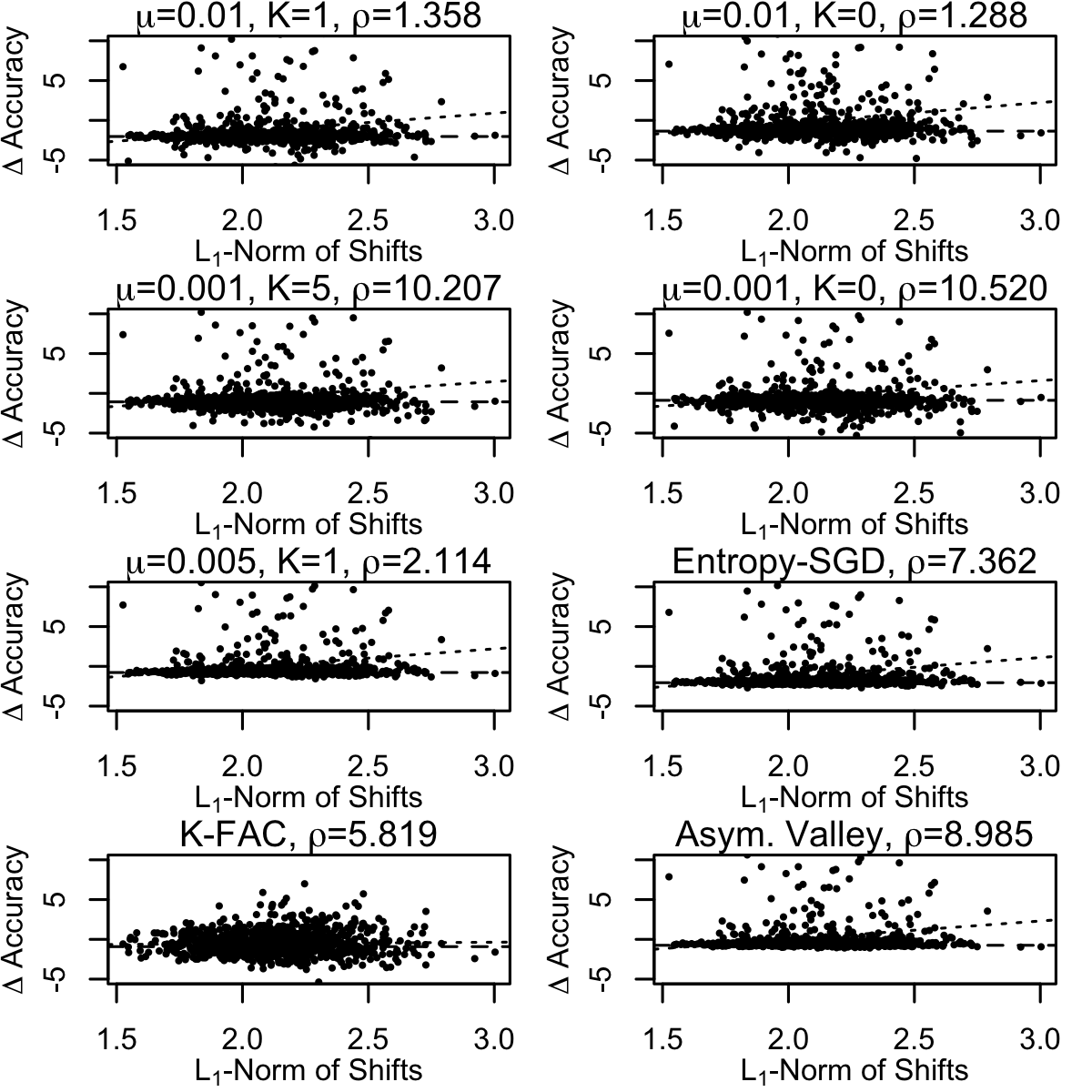
Figure 1: Difference in accuracy between regularized forest cover type models and unregularized on random mean shifts in features of test set. A horizontal dashed baseline (difference in performance on the unnmodified test set) and diagonal dotted trend line are displayed for reference.

5.2 Results

We trained a feed forward neural network on the forest cover type data, using different regularization parameters $\mu$ and $K$ and compared the accuracy on the randomly shifted test set to that of unregularized, Entropy-SGD, K-FAC, and asymmetric valley models. Figure 1 shows that there is a benefit to the regularized models and comparison models, as the $L_{1}$-norm of the shifts increases, over the unregularized model, but no significant benefit to the K-FAC model. However, there is variability in the different shifts, since all $R^{2}$ values are less than $.0204$. While these plots help visualize our comparisons, Table 2 gives us a more detailed picture: while the unregularized model is more accurate on the unshifted test data, it performs significantly worse as the $L_{1}$-norm of the shifts increases. On the other hand, the regularized, Entropy-SGD, and asymmetric valley models perform about the same, irregardless of these shifts. The slope of the trend line comparing the accuracy to the $L_{1}$-norm of the shifts is not significantly different from 0 for the regularized models, but significantly negative for the unregularized model (using a p-value of 0.05). While there are some differences between the various regularized models – there is some delineation between those with lower $\rho$ and higher – all perform better than the unregularized model. The regularized models have a significantly larger slope compared to that of the unregularized model, and the order of the slopes (from high-to-low) follows the models’ regularization strictness. Additionally, our spectral radius measure $\rho$ largely follows the regulation strictness. In terms of the regression slope, our strictest regularized models with $\mu=0.01$ and small $\rho\approx 1$ are the best and third-best performing model. Entropy-SGD is the second-best performing model, although the difference between it and the prior two models is insignificant.

Model	$\rho$	Test	AT 1	AT 2
Unregularized	21.91	94.92	85.50	63.43
Entropy-SGD	1.63	95.81	89.19	65.12
K-FAC	6.20	94.47	86.15	61.98
Asym. Valley	9.85	94.77	89.59	67.81
$\mu=0.001,K=0$	3.43	95.37	89.49	67.02
$\mu=0.005,K=0$	1.34	95.91	90.93	69.61
$\mu=0.01,K=0$	2.72	94.77	87.79	66.77
$\mu=0.02,K=0$	0.97	94.87	87.54	66.17
$\mu=0.03,K=0$	1.59	94.57	89.54	66.77
$\mu=0.05,K=1$	1.01	95.32	90.58	68.21
$\mu=0.1,K=2$	1.77	95.12	88.70	67.02

Table 3: Accuracy of models trained on USPS data. Augmented Test (AT) 1 uses random crops of up to one pixel and random rotations of up to 15^∘. Augmented Test 2 uses crops of up to two pixels and rotations of up to 30^∘.

Model	Chest X-Ray	Chest X-Ray (6 classes)	CheXpert (Validation)	MIMIC-CXR (Validation)	CheXpert (Training)	MIMIC-CXR (Training)
CheXNet	.8712	.8658	.6608	.6717	.5689	.6580
Entropy-SGD	.8239	.8348	.6565	.6688	.5570	.6577
K-FAC	.8571	.8533	.6622	.6867	.5723	.6750
$\mu=10^{-6}$	.8254	.8342	.6606	.6767	.5571	.6548
$\mu=10^{-5}$	.8255	.8340	.6749	.6838	.5621	.6635
$\mu=10^{-4}$	.8162	.8286	.6900	.6972	.5724	.6724
$\mu=5*10^{-4}$	.6695	.6569	.6230	.5486	.5509	.5707

Table 4: Mean Test AUC of Models Trained on Chest X-Ray Data

We trained a convolutional neural network on the USPS data, with no regularization; Entropy-SGD, K-FAC, and asymmetric valley methods; and various values of regularization parameters $\mu$ and $K$, comparing the accuracy on both the test and augmented test data sets. Per Table 3, while the models performed comparably on the test data (all models had an accuracy of 94.47-95.91%), our regularized models performed significantly better than the unregularized model on both augmented test data sets (87.54-90.93% vs. 85.50% on the Augmented Test 1; 66.17-69.61% vs. 63.43% on Augmented Test 2). On all test sets, the regularized model with $\mu=0.005$ and $K=0$ was the most accurate. Of our comparison models, the asymmetric valleys model performed best, only 1.5% and 2.6% worse than our best model on the augmented test sets. The Entropy-SGD model had a comparable accuracy to our regularized models on the Augmented Test 1 sets (only 1.9% worse than our best model), but it performed worse on the trickier Augmented Test 2 (6.5% worse than our best model, however, still better than the unregularized model). The K-FAC model performed worse on both augmented test sets: 5.3% worse than our best model on Augmented Test 1 and 11.0% worse on Augmented Test 2.

For the chest X-ray comparisons, we started with Zoogzog implementation of CheXNet [Rajpurkar et al., 2017], a 121-layer DenseNet trained on the chest X-ray data set as our baseline. Using this pre-trained model as the initialization, we trained for an additional epoch with our spectral radius regularization method, comparing the mean area under the curve (AUC) of the receiver of the receiver operating characteristic curve over the 14 classes (or 6 for our comparison tests). Similarly, we used this initialization and trained for one additional epoch using the Entropy-SGD and K-FAC optimization methods. The results are displayed in Table 4. Since we measured the spectral radius $\rho$ on a random batch, our batch size of four was too small to get a meaningful estimate for these models. Also, our strictest regularized model ($\mu=5*10^{-4}$) appeared to be too strictly regularized, as its test mean AUC is significantly worse than the other models. While the other regularized models performed worse in terms of test mean AUC, our regularized models performed as well or better on most of the CheXpert and MIMIC-CXR data sets, with the second-most strictly regularized model ($\mu=10^{-4}$) performing the best on these four test sets. In fact, it outperformed the original model by 4.4% and 3.8%, respectively, on the CheXpert and MIMIC-CXR “validation” sets, and 0.6% and 2.1% on the “training” sets, implying the regularized model generalizes better than the original model. K-FAC slightly outperformed this model on the MIMIC-CXR training set (by 0.4%), however performed up to 4.0% worse on the other sets. The Entropy-SGD model performed 5.9-10.2% worse than our regularized model on the CheXpert and MIMIC-CXR sets.

6 Conclusion

We created algorithms for regularized optimization of machine learning models in order to find flat minima. Furthermore, we developed tools for calculating the regularization term and its gradient for neural networks. We proved that these methods converge (or almost surely do) to a critical point. Then, we showed that the regularization works on a range of applicable problems which required us to design different methods to test generalizability for each of these problems.

Appendix A Hessian-Vector Operations Derivation

The forward computation for each layer of a network with input $x$, output $y$, weights $w$, activation $\sigma$, bias $I$, error or objective measure $E=E(y)$, and direct derivative $e_{k}=\frac{dE}{dy_{k}}$, is given by:

$$x_{k} =\sum\limits_{j}w_{ji}y_{j}$$

$$y_{k} =\sigma_{k}(x_{k})+I_{k}$$

The backward computation:

$$\frac{\partial E}{\partial y_{k}} =e_{k}(y_{k})+\sum\limits_{j}w_{ij}\frac{\partial E}{\partial x_{j}}$$

$$\frac{\partial E}{\partial x_{k}} =\sigma_{k}^{\prime}(x_{k})\frac{\partial E}{\partial y_{k}}$$

$$\frac{\partial E}{\partial w_{ij}} =y_{k}\frac{\partial E}{\partial x_{j}}$$

Applying $\mathcal{R}\left\{\cdot\right\}$ to forward pass:

$$\mathcal{R}\left\{x_{k}\right\} =\sum\limits_{j}\left(w_{ji}\mathcal{R}\left\{y_{j}\right\}+v_{ji}y_{j}\right)$$

$$\mathcal{R}\left\{y_{k}\right\} =\mathcal{R}\left\{x_{k}\right\}\sigma_{k}^{\prime}(x_{k})$$

The backwards computation follows as:

$$\mathcal{R}\left\{\frac{\partial E}{\partial y_{k}}\right\}= e_{k}^{\prime}(y_{k})\mathcal{R}\left\{y_{k}\right\}+\sum\limits_{j}\bigg{[}w_{ij}\mathcal{R}\left\{\frac{\partial E}{\partial x_{j}}\right\}$$

$$+v_{ij}\frac{\partial E}{\partial x_{j}}\bigg{]}$$

$$\mathcal{R}\left\{\frac{\partial E}{\partial x_{k}}\right\}= \sigma_{k}^{\prime}(x_{k})\mathcal{R}\left\{\frac{\partial E}{\partial y_{k}}\right\}$$

$$+\mathcal{R}\left\{x_{k}\right\}\sigma_{k}^{\prime\prime}(x_{k})\frac{\partial E}{\partial y_{k}}$$

$$\mathcal{R}\left\{\frac{\partial E}{\partial w_{ij}}\right\}= y_{k}\mathcal{R}\left\{\frac{\partial E}{\partial x_{j}}\right\}+\mathcal{R}\left\{y_{k}\right\}\frac{\partial E}{\partial x_{j}}$$

This yields the result found in Pearlmutter [1994]. However, we extend it one step further by applying $\mathcal{R}\left\{\cdot\right\}$ again, i.e., applying $\mathcal{R}^{2}\left\{\cdot\right\}=\mathcal{R}\left\{\mathcal{R}\left\{\cdot\right\}\right\}$ to the original forward pass:

$$\mathcal{R}^{2}\left\{x_{k}\right\} =\sum\limits_{j}\left(w_{ji}\mathcal{R}^{2}\left\{y_{j}\right\}+2v_{ji}\mathcal{R}\left\{y_{j}\right\}\right)$$

$$\mathcal{R}^{2}\left\{y_{k}\right\} =\mathcal{R}^{2}\left\{x_{k}\right\}\sigma_{k}^{\prime}(x_{k})+\left(\mathcal{R}\left\{x_{k}\right\}\right)^{2}\sigma_{k}^{\prime\prime}(x_{k})$$

The backwards computation follows as:

$$\mathcal{R}^{2}\left\{\frac{\partial E}{\partial y_{k}}\right\}= e_{k}^{\prime\prime}(y_{k})\left(\mathcal{R}\left\{y_{k}\right\}\right)^{2}+e_{k}^{\prime}(y_{k})\mathcal{R}^{2}\left\{y_{k}\right\}$$

$$+\sum\limits_{j}\bigg{[}w_{ij}\mathcal{R}^{2}\left\{\frac{\partial E}{\partial x_{j}}\right\}+$$

$$2v_{ij}\mathcal{R}\left\{\frac{\partial E}{\partial x_{j}}\right\}\bigg{]}$$

$$\mathcal{R}^{2}\left\{\frac{\partial E}{\partial x_{k}}\right\}= 2\mathcal{R}\left\{x_{k}\right\}\sigma_{k}^{\prime\prime}(x_{k})\mathcal{R}\left\{\frac{\partial E}{\partial y_{k}}\right\}$$

$$+\sigma_{k}^{\prime}(x_{k})\mathcal{R}^{2}\left\{\frac{\partial E}{\partial y_{k}}\right\}$$

$$+\mathcal{R}^{2}\left\{x_{k}\right\}\sigma_{k}^{\prime\prime}(x_{k})\frac{\partial E}{\partial y_{k}}$$

$$+\left(\mathcal{R}\left\{x_{k}\right\}\right)^{2}\sigma_{k}^{\prime\prime\prime}(x_{k})\frac{\partial E}{\partial y_{k}}$$

$$\mathcal{R}^{2}\left\{\frac{\partial E}{\partial w_{ij}}\right\}= 2\mathcal{R}\left\{y_{k}\right\}\mathcal{R}\left\{\frac{\partial E}{\partial x_{j}}\right\}+y_{k}\mathcal{R}^{2}\left\{\frac{\partial E}{\partial x_{j}}\right\}$$

$$+\mathcal{R}^{2}\left\{y_{k}\right\}\frac{\partial E}{\partial x_{j}}$$

The original formulation $\mathcal{R}\left\{\cdot\right\}$ allows us to efficiently compute $H(w)v$, which can be used to compute $\rho(w)$ and/or estimate the eigenvector $\bar{v}$ corresponding to the spectral radius (via Power iteration). While, the extended formulation $\mathcal{R}^{2}\left\{\cdot\right\}$ allows us to efficiently compute $v^{T}\nabla H(w)v$ and thus $\nabla\rho(w)$. This enables us to efficiently compute the gradient of our optimization problem for use in gradient descent methods.

Appendix B Analysis Proofs

B.1 Gradient Descent Convergence

Proof that the gradient descent algorithm converges (Theorem 4.1).

Proof.

Since $\nabla f$ is Lipschitz continuous (i.e., $||\nabla f(w)-\nabla f(\omega)||\leq L_{1}||w-\omega||,\ \forall\ w,\omega\in\mathbb{R}^{n}$), $-L_{1}I\preceq H(w)\preceq L_{1}I,\ \forall\ w\in\mathbb{R}^{n}$. And similarly, since $\nabla H$ is Lipschitz continuous (i.e., $||\nabla H(w)-\nabla H(\omega)||\leq L_{2}||w-\omega||,\ \forall\ w,\omega\in\mathbb{R}^{n}$), $-L_{2}I\preceq\nabla^{2}H(w)\preceq L_{2}I,\ \forall\ w\in\mathbb{R}^{n}$. We define: $h_{k}:=h(w_{k}),\ \nabla h_{k}:=\nabla h(w_{k})$.

Since our update step is $w_{k+1}=w_{k}-\alpha_{k}\nabla h_{k}$, and by applying Taylor’s Theorem:

$$h_{k+1}= f\left(w_{k}-\alpha_{k}\nabla h_{k}\right)+\mu v_{k}^{T}H\left(w_{k}-\alpha_{k}\nabla h_{k}\right)v_{k}$$

$$= h_{k}-\alpha_{k}\nabla h_{k}^{T}\nabla h_{k}+\frac{\alpha_{k}^{2}}{2}\nabla h_{k}^{T}[H(\omega)$$

$$+\mu v(\omega)^{T}\nabla^{2}H(\omega)v(\omega)]\nabla h_{k}$$

for some $\omega=\sigma w_{k}+(1-\sigma)w_{k+1}$, where $\sigma\in[0,1]$. Applying the inequality derived from Lipschitz continuity:

$$h_{k+1}\leq h_{k}-\alpha_{k}\left|\left|\nabla h_{k}\right|\right|^{2}+\frac{\alpha_{k}^{2}\left(L_{1}+\mu L_{2}\right)}{2}\left|\left|\nabla h_{k}\right|\right|^{2}$$

Given our assumption $\alpha_{k}\leq\frac{1}{L_{1}+\mu L_{2}}$,

$$\left(\frac{\alpha_{k}(L_{1}+\mu L_{2})}{2}-1\right)\alpha_{k}\leq\left(\frac{1}{2}-1\right)\alpha_{k}=-\frac{\alpha_{k}}{2}.$$

Thus:

$$h_{k+1}\leq h_{k}-\frac{\alpha_{k}}{2}\left|\left|\nabla h_{k}\right|\right|^{2}$$

Either $\left|\left|\nabla h_{k}\right|\right|=0$ or $\left|\left|\nabla h_{k}\right|\right|^{2}>0$. If the first, then the algorithm has converged to a critical point. If the second, then this step will decrease the value of the objective function. Since the objective function is bounded from below, it cannot decrease in perpetuum. Thus, it must eventually converge to a critical point. ∎

B.2 Stochastic Gradient Descent Convergence

B.2.1 Confinement and Convergence

Proof of confinement (Lemma 4.1):

Definition B.1.

$\varphi(w):=\begin{cases}0,&w<D,\\ (w-D)^{2},&w\geq D,\end{cases}$ and $\psi_{k}:=\varphi(w_{k}^{2})$.

Proof.

Definition B.1 implies that:

$$\varphi(\omega)-\varphi(w)\leq(\omega-w)\varphi^{\prime}(w)+(\omega-w)^{2},$$

for $w,\omega\in\mathbb{R}^{n}$. Note that this becomes an equality when $w,\omega>D$.

Applying this to $\psi_{k+1}-\psi_{k}$,

$$\psi_{k+1}-\psi_{k}\leq \left(-2\alpha_{k}w_{k}^{T}p_{k}+\alpha_{k}^{2}p_{k}^{2}\right)\psi^{\prime}(w_{k}^{2})$$

$$+4\alpha_{k}^{2}\left(w_{k}^{T}p_{k}\right)^{2}-4\alpha_{k}^{3}w_{k}^{T}p_{k}^{3}+\alpha_{k}^{4}p_{k}^{4}.$$

By the Cauchy-Schwartz inequality,

$$\psi_{k+1}-\psi_{k}\leq -2\alpha_{k}w_{k}^{T}p_{k}\psi^{\prime}(w_{k}^{2})+\alpha_{k}^{2}||p_{k}||^{2}\psi^{\prime}(w_{k}^{2})$$

$$+4\alpha_{k}^{2}||w_{k}||^{2}||p_{k}||^{2}-4\alpha_{k}^{3}||w_{k}||||p_{k}||^{3}$$

$$+\alpha_{k}^{4}||p_{k}||^{4}.$$

Taking the expectation,

$$\mathop{\mathbb{E}}\left[\psi_{k+1}-\psi_{k}\right]\leq -2\alpha_{k}w_{k}^{T}\nabla h_{k}\psi^{\prime}(w_{k}^{2})$$

$$+\alpha_{k}^{2}\mathop{\mathbb{E}}\left[||p_{k}||^{2}\right]\psi^{\prime}(w_{k}^{2})$$

$$+4\alpha_{k}^{2}||w_{k}||^{2}\mathop{\mathbb{E}}\left[||p_{k}||^{2}\right]$$

$$-4\alpha_{k}^{3}||w_{k}||\mathop{\mathbb{E}}\left[||p_{k}||^{3}\right]$$

$$+\alpha_{k}^{4}\mathop{\mathbb{E}}\left[||p_{k}||^{4}\right].$$

Due to Assumption 3, there exist positive constants $A_{0},B_{0}$ such that

$$\mathop{\mathbb{E}}\left[\psi_{k+1}-\psi_{k}\right]\leq -2\alpha_{k}w_{k}^{T}\nabla h_{k}\psi^{\prime}(w_{k}^{2})$$

$$+\alpha_{k}^{2}\left(A_{0}+B_{0}||w_{k}||^{4}\right),$$

and thus there exist positive constants $A,B$ such that

$$\mathop{\mathbb{E}}\left[\psi_{k+1}-\psi_{k}\right]\leq -2\alpha_{k}w_{k}^{T}\nabla h_{k}\psi^{\prime}(w_{k}^{2})$$

$$+\alpha_{k}^{2}\left(A+B\psi_{k}\right).$$

If $w_{k}^{2}<D$, then $\psi^{\prime}(w_{k}^{2})=0$, then the first term on the right hand side is zero. And if $w_{k}^{2}\geq D$, by Assumption 4, the first term of the right hand side is negative. Therefore,

$$\mathop{\mathbb{E}}\left[\psi_{k+1}-\psi_{k}\right]\leq\alpha_{k}^{2}\left(A+B\psi_{k}\right).$$

We then transform the expectation inequality to

$$\mathop{\mathbb{E}}\left[\psi_{k+1}-(1+\alpha_{k}^{2}B)\psi_{k}\right]\leq\alpha_{k}^{2}A.$$

Definition B.2.

We define the sequences $\phi_{k},\widetilde{\psi}_{k}$ as follows:

$$\phi_{k}:=\prod\limits_{i=1}^{k-1}\frac{1}{1+\alpha_{k}^{2}B}\text{ and }\widetilde{\psi}_{k}:=\phi_{k}\psi_{k}.$$

Note that $\lim\limits_{k\to\infty}\phi_{k}:=\phi_{\infty}>0$ (this can be shown by writing $\log\phi_{k}$ and using the condition on the sum of the squared learning rate). By substituting these sequences into the above inequality, we obtain

$$\mathop{\mathbb{E}}\left[\widetilde{\psi}_{k+1}-\widetilde{\psi}_{k}\right]\leq\alpha_{k}^{2}\phi_{k}A.$$

By defining $\delta_{k}(u):=\begin{cases}1,&\mathop{\mathbb{E}}\left[u_{k+1}-u_{k}\right]>0\\ 0,&\text{otherwise}\end{cases}$, for some process $u_{k}$, we can bound the positive expected variations of $\widetilde{\psi}_{k}$:

$$\mathop{\mathbb{E}}\left[\delta_{k}\left(\widetilde{\psi}\right)\right]=\mathop{\mathbb{E}}\left[\delta\mathop{\mathbb{E}}\left[\widetilde{\psi}_{k+1}-\widetilde{\psi}_{k}\right]\right]\leq\alpha_{k}^{2}\phi_{k}A.$$

Due to Assumption 2, the sum of this expectation is finite. The Quasi-Martingale Convergence Theorem states:

$$\begin{rcases}\forall k,\ u_{k}\geq 0,\\ \sum\limits_{k=1}^{\infty}\mathop{\mathbb{E}}\left[\delta_{k}(u)\right]<\infty\end{rcases}\implies u_{k}\xrightarrow[k\to\infty]{\text{a.s.}}u_{\infty}\geq 0.$$

This implies that $\widetilde{\psi}_{k}$ converges almost surely. And, since $\phi_{k}$ converges to $\phi_{\infty}>0$, $\psi_{k}$ converges almost surely.

Assume $\psi_{k}$ converges to a value $\psi_{\infty}>0$. For $k$ sufficiently large, $w_{k}^{2},w_{k+1}^{2}\geq D$. This implies that the above inequality is an equality, which then implies

$$\sum\limits_{k=1}^{\infty}\alpha_{k}w_{k}^{T}\nabla h_{k}\varphi^{\prime}(w_{k}^{2})<\infty\text{ a.s.}$$

But since $\sum\limits_{k=1}^{\infty}\alpha_{k}=\infty$ and $\varphi^{\prime}(w_{k}^{2})>0$ (for $k$ sufficiently large), this result is not compatible with Assumption 4. Because of this contradiction, we must conclude that $\psi_{k}$ converges to 0.

Since $\psi_{k}$ converges to 0, the norm $w_{k}^{2}$ and parameters $w_{k}$ are bounded. This also means that all continuous functions of $w_{k}$ are likewise bounded. ∎

Proof that SGD converges almost surely (Theorem 4.2):

Proof.

We can bound variations of loss/cost criteria $h_{k}$ using a first order Taylor expansion and bounding the second derivatives with $K_{1}$.

$$|h_{k+1}-h_{k}+2\alpha_{k}p_{k}^{T}\nabla h_{k}|\leq\alpha_{k}^{2}p_{k}^{2}K_{1}\text{ a.s.},$$

which can be rewritten as:

$$h_{k+1}-h_{k}\leq-2\alpha_{k}p_{k}^{T}\nabla h_{k}+\alpha_{k}^{2}p_{k}^{2}K_{1}\text{ a.s.}$$

Taking the expectation,

$$\mathop{\mathbb{E}}\left[h_{k+1}-h_{k}\right]\leq-2\alpha_{k}\nabla h_{k}^{2}+\alpha_{k}^{2}\mathop{\mathbb{E}}\left[p_{k}^{2}\right]K_{1}.$$

Bounding the expectation $\mathop{\mathbb{E}}\left[p_{k}^{2}\right]\leq K_{2}$, yields

$$\mathop{\mathbb{E}}\left[h_{k+1}-h_{k}\right]\leq\alpha_{k}^{2}K_{1}K_{2}.$$

Therefore, the positive expected variations are bounded by

$$\mathop{\mathbb{E}}\left[\delta_{k}\left(h\right)\right]=\mathop{\mathbb{E}}\left[\delta\mathop{\mathbb{E}}\left[h_{k+1}-h_{k}\right]\right]\leq\alpha_{k}^{2}K_{1}K_{2}.$$

By the Quasi-Martingale Convergence Theorem, $h_{k}$ converges almost surely,

$$h_{k}\xrightarrow[k\to\infty]{\text{a.s.}}h_{\infty}.$$

Additionally, taking the above and summing on $k$, implies the convergence of the following series:

$$\sum\limits_{k=1}^{\infty}\alpha_{k}\left(\nabla h_{k}\right)^{2}<\infty\text{ a.s.}$$

We define $\theta_{k}=\left(\nabla h_{k}\right)^{2}$, the variations of which are bounded using the Taylor expansion, similarly to the variations of $h_{k}$:

$$\theta_{k+1}-\theta_{k}\leq-2\alpha_{k}p_{k}^{T}\nabla^{2}h_{k}\nabla h_{k}+\alpha_{k}^{2}p_{k}^{2}K_{3}\text{ a.s.,}$$

for some constant $K_{3}$. Taking the expectation and bounding the second derivative by $K_{4}$, yields

$$\mathop{\mathbb{E}}\left[\theta_{k+1}-\theta_{k}\right]\leq\alpha_{k}\left(\nabla h_{k}\right)^{2}K_{4}+\alpha_{k}^{2}K_{2}K_{3}$$

The positive expectations are bounded,

$$\mathop{\mathbb{E}}\left[\delta_{k}\left(\theta\right)\right]= \mathop{\mathbb{E}}\left[\delta\mathop{\mathbb{E}}\left[\theta_{k+1}-\theta_{k}\right]\right]$$

$$\leq \alpha_{k}\left(\nabla h_{k}\right)^{2}K_{4}+\alpha_{k}^{2}K_{2}K_{3}$$

Since the terms on the right hand side are summands of convergent infinite sequences (by the above and the Assumption 3), by the Quasi-Martingale Convergence Theorem, $\theta_{k}$ converges almost surely. And since the above sequence converges almost surely, this implies the limit must be zero:

$$\theta_{k}\xrightarrow[k\to\infty]{\text{a.s.}}0\text{ and }\nabla h_{k}\xrightarrow[k\to\infty]{\text{a.s.}}0.$$

∎

B.2.2 Power Iteration

Proof that power iteration follows the assumed update steps (Lemma 4.2):

Proof.

For ease, we define $g_{k}=\max\{0,\rho_{k}-K\}$. We begin by splitting $p_{k}$ into its components:

$$||p_{k}||^{2}= ||p_{k}-\bar{p}_{k}+\bar{p}_{k}||^{2}$$

$$= ||p_{k}-\bar{p}_{k}||^{2}+||\bar{p}_{k}||^{2}+\left(p_{k}-\bar{p}_{k}\right)^{T}\bar{p}_{k}.$$

By the definition of $\bar{p}_{k}$ and the triangle inequality,

$$||\bar{p}_{k}||^{2}\leq||\nabla f_{k}||^{2}+2\mu_{k}||\nabla f_{k}||||\nabla g_{k}||+\mu_{k}^{2}||\nabla g_{k}||^{2}.$$

Taking the expectation and applying the Cauchy-Schwartz inequality yields:

$$\mathop{\mathbb{E}}\left[||p_{k}||^{2}\right]\leq S_{2}+\mathop{\mathbb{E}}\left[||\nabla f_{k}||^{2}\right]$$

$$+2\mu_{k}\left(\mathop{\mathbb{E}}\left[||\nabla f_{k}||^{2}\right]\right)^{\frac{1}{2}}\left(\mathop{\mathbb{E}}\left[||\nabla g_{k}||^{2}\right]\right)^{\frac{1}{2}}$$

$$+\mu_{k}^{2}\mathop{\mathbb{E}}\left[||\nabla g_{k}||^{2}\right].$$

Note $\mathop{\mathbb{E}}\left[p_{k}-\bar{p}_{k}\right]=0$. Similarly,

$$\mathop{\mathbb{E}}\left[||p_{k}||^{3}\right]\leq S_{3}+\mathop{\mathbb{E}}\left[||\nabla f_{k}||^{3}\right]$$

$$+3\mu_{k}\left(\mathop{\mathbb{E}}\left[||\nabla f_{k}||^{3}\right]\right)^{\frac{2}{3}}\left(\mathop{\mathbb{E}}\left[||\nabla g_{k}||^{3}\right]\right)^{\frac{1}{3}}$$

$$+3\mu_{k}^{2}\left(\mathop{\mathbb{E}}\left[||\nabla f_{k}||^{3}\right]\right)^{\frac{1}{3}}\left(\mathop{\mathbb{E}}\left[||\nabla g_{k}||^{3}\right]\right)^{\frac{2}{3}}$$

$$+\mu_{k}^{3}\mathop{\mathbb{E}}\left[||\nabla g_{k}||^{3}\right],$$

$$\mathop{\mathbb{E}}\left[||p_{k}||^{4}\right]\leq S_{4}+\mathop{\mathbb{E}}\left[||\nabla f_{k}||^{4}\right]$$

$$+4\mu_{k}\left(\mathop{\mathbb{E}}\left[||\nabla f_{k}||^{4}\right]\right)^{\frac{3}{4}}\left(\mathop{\mathbb{E}}\left[||\nabla g_{k}||^{4}\right]\right)^{\frac{1}{4}}$$

$$+6\mu_{k}^{2}\left(\mathop{\mathbb{E}}\left[||\nabla f_{k}||^{4}\right]\right)^{\frac{1}{2}}\left(\mathop{\mathbb{E}}\left[||\nabla g_{k}||^{4}\right]\right)^{\frac{1}{2}}$$

$$+4\mu_{k}^{3}\left(\mathop{\mathbb{E}}\left[||\nabla f_{k}||^{4}\right]\right)^{\frac{1}{4}}\left(\mathop{\mathbb{E}}\left[||\nabla g_{k}||^{4}\right]\right)^{\frac{3}{4}}$$

$$+\mu_{k}^{4}\mathop{\mathbb{E}}\left[||\nabla g_{k}||^{4}\right].$$

Given Assumption 1, we only need to show that the moments of $\nabla g_{k}$ are similarly bounded.

Next, we split $\nabla g_{k}$ into its components:

$$||\nabla g_{k}||= \left|\left|v_{k}^{T}\nabla H_{k}v_{k}\right|\right|$$

$$= \left|\left|\left(v_{k}-\bar{v}_{k}+\bar{v}_{k}\right)^{T}\nabla H_{k}\left(v_{k}-\bar{v}_{k}+\bar{v}_{k}\right)\right|\right|.$$

By expanding and applying the triangle inequality,

$$||\nabla g_{k}||\leq \left|\left|\left(v_{k}-\bar{v}_{k}\right)^{T}\nabla H_{k}\left(v_{k}-\bar{v}_{k}\right)\right|\right|$$

$$+2\left|\left|\left(v_{k}-\bar{v}_{k}\right)^{T}\nabla H_{k}\bar{v}_{k}\right|\right|+\left|\left|\bar{v}_{k}^{T}\nabla H_{k}\bar{v}_{k}\right|\right|.$$

Applying Assumption 2 and 3 (including $||H(w)-H(\omega)||\leq L||w-\omega||,\ \forall\ w,\omega\in\mathbb{R}^{n}$),

$$||\nabla g_{k}||\leq\varepsilon^{2}L+2\varepsilon\left|\left|\nabla H_{k}\bar{v}_{k}\right|\right|+\left|\left|\bar{v}_{k}^{T}\nabla H_{k}\bar{v}_{k}\right|\right|.$$

This implies that, for $j=2,3,4$,

$$\mathop{\mathbb{E}}\left[||\nabla g_{k}||^{j}\right]\leq\widetilde{A}_{j}+\widetilde{B}_{j}\mathop{\mathbb{E}}\left[\left|\left|\bar{v}_{k}^{T}\nabla H_{k}\bar{v}_{k}\right|\right|^{j}\right]$$

where $\widetilde{A}_{j},\widetilde{B}_{j}$ are some positive constants. Given Assumption 1, this implies that

$$\mathop{\mathbb{E}}\left[||\nabla g_{k}||^{j}\right]\leq\overline{A}_{j}+\overline{B}_{j}||w_{k}||^{j},$$

for $j=2,3,4$ and some positive constants $\overline{A}_{j},\overline{B}_{j}$. Combining this with the above results, shows that the second, third, and fourth moments of the update term are bounded as required. ∎

Proof of of conditions on Epsilon (Lemma 4.3):

Proof.

We start by splitting $v_{k}^{T}\nabla H_{k}v_{k}$ into its components:

$$v_{k}^{T}\nabla H_{k}v_{k}= (v_{k}-\bar{v}_{k}+\bar{v}_{k})^{T}\nabla H_{k}(v_{k}-\bar{v}_{k}+\bar{v}_{k})$$

$$= (v_{k}-\bar{v}_{k})^{T}\nabla H_{k}(v_{k}-\bar{v}_{k})$$

$$+2(v_{k}-\bar{v}_{k})^{T}\nabla H_{k}\bar{v}_{k}+\bar{v}_{k}^{T}\nabla H_{k}\bar{v}_{k}.$$

Taking the expectation, the last term $\mathop{\mathbb{E}}\left[\bar{v}_{k}^{T}\nabla H_{k}\bar{v}_{k}\right]=\nabla\bar{g}_{k}$ by definition. Since $\mathop{\mathbb{E}}\left[v_{k}-\bar{v}_{k}\right]=0$, and the other values in second term are fixed, $\mathop{\mathbb{E}}\left[(v_{k}-\bar{v}_{k})^{T}\nabla H_{k}\bar{v}_{k}\right]=0$. However, we must examine the first term further (as we will get a term proportional to the square error):

$$\left|\left|\mathop{\mathbb{E}}\left[(v_{k}-\bar{v}_{k})^{T}\nabla H_{k}(v_{k}-\bar{v}_{k})\right]\right|\right|\leq L\mathop{\mathbb{E}}\left[\left|\left|v_{k}-\bar{v}_{k}\right|\right|^{2}\right]$$

$$\leq L\varepsilon^{2}.$$

If $\varepsilon\to 0$ as $k\to\infty$, then the expectation $\mathop{\mathbb{E}}\left[v_{k}^{T}\nabla H_{k}v_{k}\right]=\mathop{\mathbb{E}}\left[\bar{v}_{k}^{T}\nabla H_{k}\bar{v}_{k}\right]=\nabla\bar{g}_{k}$. ∎

Appendix C Experiments

C.1 Data Sets

The forest cover type data uses cartographic data to predict the tree species (as determined by the United States Forest Service) of a 30 x 30 meter cell. This cartographic data includes: elevation, aspect, slope, distance to surface water features, distance to roadways, hillshade index at three times of day, distance to wildfire ignition points, wilderness area designation, and soil type. Seven major tree species are included: spruce/fir, lodgepole pine, Ponderosa pine, cottonwood/willow, aspen, Douglis-fir, and krummholz. 581,012 samples are included, which we split 64%/16%/20% into train/validation/test data sets.

The USPS digits data includes 16 x 16 pixels greyscale images from scanned envelopes, with the goal to identify which digit 0-9 each image corresponds to. This data set is already split 7,291 training and 2,007 test images. We take 1/7 of the training set as validation.

The chest X-ray data contains 1024 x 1024 pixels color images of patients’ chest x-rays, and identifying which of fourteen lung diseases each patient has: atelectasis, cardiomegaly, effusion, infiltration, mass, nodule, pneumonia, pneumothorax, consolidation, edema, emphysema, fibrosis, pleural thickening, and hernia. Note that this is a multi-label problem: patients can have none, one, or multiple of these conditions. 112,120 images are included, which we split 70%/10%/20% into train/validation/test data sets.

C.2 Generalization Tests

For the forest cover type data, we weighted the test subjects in order to shift the mean of a feature or multiple features. Since we normalized our data, the weight of each test subject was determined by the ratio of the normal probability distribution function value with the shift and the value without the shift. This shift adds a slight bias to the test set that was not in the original data set, while maintaining real feature values. In practice, we first increased the mean of each feature value by 0.1, using this shift method, compared the accuracy of our trained models, and found that certain features were problematic. Upon further examination, this was because these features were binary factors with rare classes (so our weighting of subjects put all of the emphasis on a few of them). Then, we shifted each of the features (except the problematic modes) by a random normal amount (with mean 0 and standard deviation 0.05), compared the accuracy of our trained models, and repeated for a total of one thousand times.

For the USPS handwritten digits data, we augmented the test set: Augmented Test 1 used random crops (with padding) of up to one pixel and random rotations of up to 15^∘; Augmented Test 2 used crops of up to two pixels and rotations of up to 30^∘. Note that we did not augment our training set while learning our models, as a similar augmentation would yield comparable training and test sets.

For the chest X-ray data, we compared performance on two similar data sets, CheXpert [Irvin et al., 2019] and MIMIC-CXR [Johnson et al., 2019]. For this comparison, we only considered the six conditions common to the three data sets: atelectasis, cardiomegaly, consolidation, edema, pneumonia, and pneumothorax. Additionally, we ignored any uncertain labels in the CheXpert and MIMIC-CXR classes. We kept the assigned training and validation data sets separate for each data set, as there appeared to be differences in labeling. Particularly, the CheXpert validation set appears to be fully labeled, while the training set contains uncertain and missing labels. While these are labeled “training” and “validation” sets, we solely used them as test sets. MIMIC-CXR contains 2,732 validation and 369,188 training images. CheXpert contains 234 validation and 223,415 training images.

C.3 Implementation

A Github link to our code will be provided by publication.

For the forest cover type models, we trained using stochastic gradient descent, with learning rate $\frac{0.5}{\text{epoch \#}}$, batch-size of 128, and a maximum of 100 epochs and 10,000 power iterations. The network used 3 hidden layers with 20 hidden nodes in each layer.

For the USPS models, we used the Adam optimizer, with learning rate of $10^{-3}$, batch-size of 128, and a maximum of 100 epochs and 10,000 power iterations. The network took an input image, and processed it through the following layers in order: convolution to 8 channels, pool, convolution to 16 channels, pool, convolution to 32 channels, pool, fully connected to 64 nodes, fully connected to 10 nodes, softmax. All convolutions were of kernel size 3, stride 1, and padding 1; all pools were max pooling with kernel size 2 and stride 2. ReLUs were used to connect the various layers.

For the chest X-ray models, we resized the images to 256 x 256, then crop to 224 x 224. We used the Adam optimizer, with learning rate of $10^{-5}$, batch-size of 4, and a maximum of 100 power iterations. We also tried 5 epochs, however the first epoch had the highest validation mean AUC. We kept regularization parameter $K=0$.

The Entropy-SGD models were trained with a learning rate of 0.1 (except on the chest x-ray data, where 0.001 was used), momentum of 0.9, and no dampening or weight decay. The K-FAC models were trained using alecwangcq implementation, with a learning rate of 0.001 (except on the chest x-ray data, where $10^{-7}$ was used) and momentum of 0.9.

The Asymmetric Valley models were trained with an initial learning rate of 0.5, and trained for 250 epochs (iterations 161-200 utilizing stochastic weight averaging).

References

- Aa, van der et al. [2007] N.P. Aa, van der, H.G. Morsche, ter, and R.M.M. Mattheij. Computation of eigenvalue and eigenvector derivatives for a general complex-valued eigensystem. Electronic Journal of Linear Algebra, 16:300–314, 2007. ISSN 1081-3810.
- Blackard and Dean [1999] J A Blackard and D J Dean. Comparative accuracies of artificial neural networks and discriminant analysis in predicting forest cover types from cartographic variables. Computers and Electronics in Agriculture, vol.24:131–151, 1999.
- Bottou [1998] Léon Bottou. On-line learning and stochastic approximations. In In On-line Learning in Neural Networks, pages 9–42. Cambridge University Press, 1998.
- Chaudhari et al. [2016] Pratik Chaudhari, Anna Choromanska, Stefano Soatto, Yann LeCun, Carlo Baldassi, Christian Borgs, Jennifer T. Chayes, Levent Sagun, and Riccardo Zecchina. Entropy-sgd: Biasing gradient descent into wide valleys. CoRR, abs/1611.01838, 2016. URL http://arxiv.org/abs/1611.01838.
- G. [2018] Andrey G. zoogzog/chexnet, 2018. URL https://github.com/zoogzog/chexnet.
- He et al. [2019] Haowei He, Gao Huang, and Yang Yuan. Asymmetric valleys: Beyond sharp and flat local minima. In H. Wallach, H. Larochelle, A. Beygelzimer, F. d’Alché Buc, E. Fox, and R. Garnett, editors, Advances in Neural Information Processing Systems, volume 32, pages 2553–2564. Curran Associates, Inc., 2019. URL https://proceedings.neurips.cc/paper/2019/file/01d8bae291b1e4724443375634ccfa0e-Paper.pdf.
- Irvin et al. [2019] Jeremy Irvin, Pranav Rajpurkar, Michael Ko, Yifan Yu, Silviana Ciurea-Ilcus, Chris Chute, Henrik Marklund, Behzad Haghgoo, Robyn L. Ball, Katie S. Shpanskaya, Jayne Seekins, David A. Mong, Safwan S. Halabi, Jesse K. Sandberg, Ricky Jones, David B. Larson, Curtis P. Langlotz, Bhavik N. Patel, Matthew P. Lungren, and Andrew Y. Ng. Chexpert: A large chest radiograph dataset with uncertainty labels and expert comparison. CoRR, abs/1901.07031, 2019. URL http://arxiv.org/abs/1901.07031.
- Jastrzebski et al. [2018] Stanisław Jastrzebski, Zachary Kenton, Devansh Arpit, Nicolas Ballas, Asja Fischer, Yoshua Bengio, and Amos Storkey. Finding flatter minima with sgd, 2018. URL https://openreview.net/forum?id=r1VF9dCUG.
- Johnson et al. [2019] Alistair E. W. Johnson, Tom J. Pollard, Seth J. Berkowitz, Nathaniel R. Greenbaum, Matthew P. Lungren, Chih-ying Deng, Roger G. Mark, and Steven Horng. MIMIC-CXR: A large publicly available database of labeled chest radiographs. CoRR, abs/1901.07042, 2019. URL http://arxiv.org/abs/1901.07042.
- Keskar et al. [2016] Nitish Shirish Keskar, Dheevatsa Mudigere, Jorge Nocedal, Mikhail Smelyanskiy, and Ping Tak Peter Tang. On large-batch training for deep learning: Generalization gap and sharp minima. CoRR, abs/1609.04836, 2016. URL http://arxiv.org/abs/1609.04836.
- LeCun et al. [1990] Yann LeCun, O. Matan, B. Boser, J. S. Denker, D. Henderson, R. E. Howard, W. Hubbard, L. D. Jackel, and H. S. Baird. Handwritten zip code recognition with multilayer networks. In Proceedings - International Conference on Pattern Recognition, volume 2, pages 35–40. Publ by IEEE, 1990.
- Ma et al. [2019] Linjian Ma, Gabe Montague, Jiayu Ye, Zhewei Yao, Amir Gholami, Kurt Keutzer, and Michael W. Mahoney. Inefficiency of K-FAC for large batch size training. CoRR, abs/1903.06237, 2019. URL http://arxiv.org/abs/1903.06237.
- Martens and Grosse [2015] James Martens and Roger B. Grosse. Optimizing neural networks with kronecker-factored approximate curvature. CoRR, abs/1503.05671, 2015. URL http://arxiv.org/abs/1503.05671.
- Pearlmutter [1994] Barak A. Pearlmutter. Fast exact multiplication by the hessian. Neural Computation, 6:147–160, 1994.
- Rajpurkar et al. [2017] Pranav Rajpurkar, Jeremy Irvin, Kaylie Zhu, Brandon Yang, Hershel Mehta, Tony Duan, Daisy Yi Ding, Aarti Bagul, Curtis Langlotz, Katie S. Shpanskaya, Matthew P. Lungren, and Andrew Y. Ng. Chexnet: Radiologist-level pneumonia detection on chest x-rays with deep learning. CoRR, abs/1711.05225, 2017. URL http://arxiv.org/abs/1711.05225.
- Wang [2019] Chaoqi Wang. alecwangcq/kfac-pytorch, 2019. URL https://github.com/alecwangcq/KFAC-Pytorch.
- Wang et al. [2017] Xiaosong Wang, Yifan Peng, Le Lu, Zhiyong Lu, Mohammadhadi Bagheri, and Ronald Summers. Chestx-ray8: Hospital-scale chest x-ray database and benchmarks on weakly-supervised classification and localization of common thorax diseases. In 2017 IEEE Conference on Computer Vision and Pattern Recognition (CVPR), pages 3462–3471, 2017.
- Yao et al. [2018] Zhewei Yao, Amir Gholami, Qi Lei, Kurt Keutzer, and Michael W. Mahoney. Hessian-based analysis of large batch training and robustness to adversaries, 2018.
- Yoshida and Miyato [2017] Yuichi Yoshida and Takeru Miyato. Spectral norm regularization for improving the generalizability of deep learning, 2017.