On Theoretical and Numerical Aspect of Fractional Differential Equations with Purely Integral Conditions

Abstract.

In this paper, we are interested in the study of a problem with fractional derivatives having boundary conditions of integral types. The problem represents a Caputo type advection-diffusion equation where the fractional order derivative with respect to time with $1<\alpha<2$. The method of the energy inequalities is used to prove the existence and the uniqueness of solutions of the problem. The finite difference method is also introduced to study the problem numerically in order to find an approximate solution of the considered problem. Some numerical examples are presented to show satisfactory results.

1. Introduction

Fractional Partial Differential Equations (FPDE) are considered as generalizations of partial differential equations having an arbitrary order and play essential role in engineering, physics and applied mathematics. Due to the properties of Fractional Differential Equations $\left(\text{FDE}\right)$, the non-local relationships in space and time are used to model a complex phenomena, such as in electroanalytical chemistry, viscoelasticity $[10,21]$, porous environment, fluid flow, thermodynamic $[11,34,35]$, diffusion transport, rheology $\left[5,7,15,26,31,33\right]$, electromagnetism, signal processing $[20,21,30]$, electrical network $[20]$ and others $[9,13,26,27]$. Several problems have been studied in modern physics and technology by using the partial differential equations (PDEs) where the nonlocal conditions were described by integrals, further these integral conditions are of great interest due to their applications in population dynamics, models of blood circulation, chemical engineering thermoelasticity $[34]$. At the same time, the existence and uniqueness of the solutions for these type of problems have been studied by several researchers, see for example $[2,12,16,27,28,29]$. Some results have been obtained by construction of variational formulation and depends on the choice of spaces along their norms, Lax-Milgram theorem, Poincaré theorem, fixed point theory. For the numerical studies of (EDPF) with classical boundary nonlocal conditions, we can cite the works of A. Alikhanov $[3,5,6,7]$, Meerschaert $[15]$, Shen and Liu $[26]$ and many others.

In this study, we are interested in a problem (FPDE) with boundary conditions of integrals type $\displaystyle\int_{0}^{1}v\left(x,t\right)dx,$ $\displaystyle\int_{0}^{1}x^{n}v\left(x,t\right)dx$. For the theoretical study, we use the energy inequalities method to prove the existence and the uniqueness. However the numerical study is based on the finite difference method to obtain an approximate numerical solution of the proposed problem. We use a uniform discretization of space and time and the fractional operator in the Caputo sense having order $\alpha$ $(1<\alpha<2)$ is approximated by a scheme called $L2$ $[26]$, similarly the integer-order differential operators are also approximated by central and advanced numerical schemes. For the stability and convergence of obtained numerical scheme, the conditionally stable method is used and we prove the convergence. Numerical tests are carried out in order to illustrate satisfactory results from the point of view that the values of the approximate solution that is very close to the exact solution. In the process of numerical and graphical results we applied MATLAB software..

1.1. Notions and preleminaries

In this section we recall some early results that we need, such as, the definition of Caputo derivative to explain the problem that we shall study in this work: let $\Gamma\left(.\right)$ denote the gamma function. For any positive non-integer value $1<\alpha<2,$ the caputo derivative defined as follows:

Definition 1.

$\left(See\text{ }\left[12\right]\right).$ Let us denote by $C_{0}\left(0,1\right)$ the space of continuous fonctions with compact support in $\left(0,1\right),$ and its bilinear form is given by

$$\left(\left(u,w\right)\right)=\mathop{\displaystyle\int}\limits_{0}^{1}\Im_{x}^{m}u.\Im_{x}^{m}wdx\text{ \ \ \ \ \ \ \ \ }\left(m\in\mathbb{N}^{\ast}\right),$$ (1)

where

$$\Im_{x}^{m}u=\mathop{\displaystyle\int}\limits_{0}^{x}\frac{\left(x-\xi\right)^{m-1}}{\left(m-1\right)!}u\left(\xi,t\right)d\xi\ \ \ \ \ \ \ \ \left(m\in\mathbb{N}^{\ast}\right).$$

For $m=1$, we have $\Im_{x}u=\mathop{\displaystyle\int}\limits_{0}^{x}u\left(\xi,t\right)d\xi$ and $\Im_{t}u=\mathop{\displaystyle\int}\limits_{0}^{t}u\left(x,\tau\right)d\tau.$ The bilinear form $\left(\ref{66}\right)$ is considered as scalar product on $C_{0}\left(0,1\right)$ when is not complete.

Definition 2.

$\left(See\text{ }\left[12\right]\right).$ We denote  by

$$B_{2}^{m}\left(0,1\right)=\left\{\begin{array}[]{c}L^{2}\left(0,1\right)\text{ \ \ \ \ \ \ \ \ \ \ \ \ \ \ \ \ }for\text{ }m=0\\ u/\Im_{x}^{m}u\in L^{2}\left(0,1\right)\text{ \ }\ \text{\ \ \ }for\text{ }m\in\mathbb{N}^{\ast},\end{array}\right.$$

the completion of $C_{0}\left(0,1\right)$ for the scalar product defined by $\left(\ref{66}\right)$.The associated norm to the scalar product is given by

$$\left\|u\right\|_{B_{2}^{m}\left(0,1\right)}=\left\|\Im_{x}^{m}u\right\|_{L^{2}\left(0,1\right)}=\left(\mathop{\displaystyle\int}\limits_{0}^{T}\left(\Im_{x}^{m}u\right)^{2}dx\right)^{\frac{1}{2}}.$$

Lemma 3.

$\left(See\text{ }\left[8\right]\right).$ For all $m\in\mathbb{N}^{\ast},$ we obtain

$$\left\|u\right\|_{B_{2}^{m}\left(0,1\right)}\leq\left(\frac{1}{2}\right)^{m}\left\|u\right\|_{L^{2}\left(0,1\right)}^{2}.$$ (2)

Definition 4.

$\left(See\text{ }\left[12\right]\right).$ Let $X$ be a Banach space with the norm $\left\|u\right\|_{X}$ , and let u :$\left(0,T\right)\rightarrow X$ be an abstract functions, by $\left\|u\left(.,t\right)\right\|_{X}$ we denote the norm of the element $u\left(.,t\right)\in X$ at a fixed t.

We denote by $L^{2}\left(0,T;X\right)$ the set of all measurable abstract functions $u\left(.,t\right)$ from $\left(0,T\right)$ into $X$ such that

$$\left\|u\right\|_{L^{2}\left(0,T;X\right)}=\left(\mathop{\displaystyle\int}\limits_{0}^{T}\left\|u\left(.,t\right)\right\|_{X}dt\right)^{\frac{1}{2}}<\infty.$$

Lemma 5.

$\left[\text{Cauchy inequality with }\varepsilon\right]\left(See\text{ }\left[13\right]\right).$ For all $\varepsilon$ and arbitrary variables a,b$\in\mathbb{R},$ we have the following inequality:

$$\left|ab\right|\leq\frac{\varepsilon}{2}\left|a\right|^{2}+\frac{1}{2\varepsilon}\left|b\right|^{2}.$$ (3)

Definition 6.

$\left(See\text{ }\left[21\right]\right).$ The left Caputo derivative for $1<$ $\alpha<2$ can be expressed as

$${}_{0}^{c}\partial_{t}^{\alpha}f\left(t\right)=\frac{1}{\Gamma\left(2-\alpha\right)}\mathop{\displaystyle\int}\limits_{0}^{t}\frac{f\text{ }"\left(s\right)}{\left(t-s\right)^{\alpha-1}}ds;\text{ }t>0.$$

Definition 7.

$\left(See\text{ }\left[21\right]\right).$ The integral of order $\alpha$ of the function $f\in L^{1}\left[a,b\right]$ is defined by:

$$I_{0}^{\alpha}f\left(t\right)=\frac{1}{\Gamma\left(\alpha\right)}\mathop{\displaystyle\int}\limits_{0}^{t}\frac{f\left(s\right)}{\left(t-s\right)^{1-\alpha}}ds;\text{ }t>0.$$

Lemma 8.

$\left(See\text{ }\left[1\right]\right).$ For all real $1<$ $\alpha<2$ we have the inequality

$$\int_{0}^{1}\,{}_{0}^{c}\partial_{t}^{\alpha}\left(\Im_{x}u\right)^{2}dx\leq 2\int_{0}^{1}\left({}_{0}^{c}\partial_{t}^{\alpha}u\right)\left(\Im_{x}u\right)dx.$$

Lemma 9.

$\left(See\text{ }\left[28\right]\right).$ For all real $1<$ $\alpha<2$ we have the inequality

$$\int_{Q}\,\left({}_{0}^{c}\partial_{t}^{\alpha}u\right)\left(\Im_{x}u\right)dxdt\leq\int_{Q}\left({}_{0}^{c}\partial_{t}^{\frac{\alpha}{2}}\Im_{x}u\right)^{2}dxdt.$$

2. Statement of the problem

In the rectangular domain

$$Q=\left\{(x,t)\in\mathbb{R}^{2}:0<x<1,\text{ }0<t<T\right\}\text{, \ where }T>0,$$

we consider the fractional differential equation:

$$\pounds v={}_{0}^{c}\partial_{t}^{\alpha}v+a(x,t)\frac{\partial^{2}v}{\partial x^{2}}+b(x,t)\frac{\partial v}{\partial x}+c\left(x,t\right)v=g\left(x,t\right),\text{ where }1<\alpha<2,$$ (4)

to the equation $(\ref{1})$, we associate the initial conditions:

$$\left\{\begin{array}[]{c}\ell v=v(x,0)=\Phi(x),\qquad\,x\in(0,1),\\ \displaystyle qv=\frac{v(x,0)}{\partial t}=\Psi(x),\,\qquad x\in(0,1),\end{array}\right.$$ (5)

and the purely integrals conditions

$$\left\{\begin{array}[]{c}\displaystyle\int_{0}^{1}v\left(x,t\right)dx=\mu(t),\qquad t\in(0,T),\\ \displaystyle\int_{0}^{1}xv\left(x,t\right)dx=E(t),\qquad t\in(0,T),\end{array}\right.$$ (6)

where $\Phi,\Psi,\mu,E,a,b,c$ and $g$ are  known continuous functions.

Assumptions:

1) for all $(x,t)\in\overline{Q}$, we assume that:

$$\underset{Q}{\sup\ }a(x,t)\leq 0,\underset{Q}{\sup}\frac{\partial a^{4}(x,t)}{\partial x^{4}}\geq 0,\underset{Q}{\inf}\frac{\partial^{3}b(x,t)}{\partial x^{3}}\leq 0,c(x,t)\geq 0,\underset{Q}{\sup}\frac{\partial c^{2}(x,t)}{\partial x^{2}}\geq 0,$$ (7)

2) for all $(x,t)\in\overline{Q}$, we assume that:

$$\ 0<M \leq 4\frac{\partial^{2}a(x,t)}{\partial x^{2}}-4\underset{Q}{\sup}a(x,t)-\frac{1}{2}\underset{Q}{\sup}\frac{\partial a^{4}(x,t)}{\partial x^{4}}+\frac{1}{2}\underset{Q}{\inf}\frac{\partial^{3}b(x,t)}{\partial x^{3}}$$ (8)

$$\hskip 28.90755pt-\frac{1}{2}\underset{Q}{\sup}\frac{\partial c^{2}(x,t)}{\partial x^{2}}-3\frac{\partial b(x,t)}{\partial x}+2c\left(x,t\right)-\frac{1}{2\varepsilon}.$$

3$)$ The functions $\Phi(x)$ and $\Psi(x)$ satisfy the following compatibility conditions:

$$\int_{0}^{1}\Phi dx=\mu(0),\,\int_{0}^{1}x\Phi dx=E(0),\int_{0}^{1}\Psi dx=\mu^{\prime}(0),\,\int_{0}^{1}x\Psi dx=E^{\prime}(0).$$ (9)

We transform a problem $\left(\ref{1}\right)$ – $\left(\ref{3}\right)$ with nonhomegenous integral conditions to the equivalent problem with homogenous integral conditions, by introducing a new unknown function $u$ defined by

$$v(x,t)=\widetilde{u}(x,t)+U(x,t),$$ (10)

where

$$U(x,t)=2(2-3x)\mu(t)+6(2x-1)E(t).$$ (11)

Now we study a new problem with homegenous integral conditions

$$\left\{\begin{array}[]{c}\displaystyle\pounds\widetilde{u}=_{0}^{c}\partial_{t}^{\alpha}\widetilde{u}+a(x,t)\frac{\partial^{2}\widetilde{u}}{\partial x^{2}}+b(x,t)\frac{\partial\widetilde{u}}{\partial x}+c\left(x,t\right)\widetilde{u}=h\left(x,t\right),\\ \displaystyle\ell v=\widetilde{u}(x,0)=\varphi(x),\qquad x\in(0,1),\\ \displaystyle qv=\frac{\widetilde{u}(x,0)}{\partial t}=\psi(x),\qquad x\in(0,1),\\ \displaystyle\int_{0}^{1}\widetilde{u}\left(x,t\right)dx=0,\qquad\,t\in(0,T),\\ \displaystyle\int_{0}^{1}x\widetilde{u}\left(x,t\right)dx=0,\,\qquad t\in(0,T),\end{array}\right.$$ (12)

where

$$h(x,t) = g(x,t)-\pounds{\normalsize U}(x,t),$$

$$\varphi(x) = \Phi(x)-\ell{\normalsize U},$$

$$\psi(x) = \Psi(x)-q{\normalsize U}$$

and

$$\int_{0}^{1}\varphi(x)dx=0,\,\int_{0}^{1}x\varphi(x)dx=0,\int_{0}^{1}\psi(x)=0,\,\int_{0}^{1}x\psi(x)=0.$$

Again we introduce new function $u$ defined by

$$u(x,t)=\widetilde{u}(x,t)-\psi\left(x\right)t-\varphi\left(x\right),$$ (13)

therefore the problem $\left(\ref{9}\right)$ can be given as follow

$$\left\{\begin{array}[]{c}\pounds u={}_{0}^{c}\partial_{t}^{\alpha}u+a(x,t)\frac{\partial^{2}u}{\partial x^{2}}+b(x,t)\frac{\partial u}{\partial x}+c\left(x,t\right)u=f\left(x,t\right),\\ \displaystyle\ell u=u(x,0)=0,\,\qquad x\in(0,1),\\ \displaystyle qu=\frac{u(x,0)}{\partial t}=0,\qquad\,x\in(0,1),\\ \displaystyle\int_{0}^{1}u(x,t)dx=0,\qquad\,t\in(0,T),\\ \displaystyle\int_{0}^{1}xu(x,t)dx=0,\qquad\,\,t\in(0,T).\end{array}\right.$$ (14)

Thus, instead of seeking a solution $v$ of the problem $\left(\ref{1}\right)-\left(\ref{3}\right)$, we establish the existence and uniqueness of solution $u$ of the problem $\left(\ref{11}\right)$ and solution $v$ will simply be given by:

$$v(x,t)=\widetilde{u}(x,t)+U(x,t).$$ (15)

3. Inequality of energy and its consequences

The solution of the problem $\left(\ref{11}\right)$ can be considered as a solution of the problem in operational form:

$$Lu=\tciFourier,$$

where $L=(\pounds,\ell,q)$ is considered from $B$ to $F$, where $B$ is a Banach space of functions $u\in L{{}^{2}}(Q)$, whose norm:

$$\left\|u\right\|_{B}=\left(\int_{Q}\left({}_{0}^{c}\partial_{t}^{\frac{\alpha}{2}}\left(\Im_{x}u\right)\right)^{2}dxdt+\int_{Q}\left(\Im_{x}u\right)^{2}dxdt\right)^{\frac{1}{2}}$$ (16)

is finite, and $F$ is a Hilbert space consisting of all the elements $F=$ $\left(f,0,0\right)$ whose norm is given by:

$$\left\|\tciFourier\right\|_{F}=\left(\int_{Q}\text{\ }f^{\text{ }2}dxdt\right)^{\frac{1}{2}}.$$ (17)

Now we let $D(L)$ be the domain of  the opérator $L$ for the set of all functions $u$ such as that: $\Im_{x}u,$ $\Im_{x}\left({}_{0}^{c}\partial_{t}^{\alpha}u\right),$ $\Im_{x}\frac{\partial u}{\partial x},$ $\Im_{x}\frac{\partial^{2}u}{\partial x^{2}}\in L^{2}(Q)$ and $u$ satisfies the integral conditions in problem $\left(\ref{11}\right).$ Then,

Theorem 10.

Under assumptions $\left(\ref{4a}\right)$-$\left(\ref{5a}\right)$, the condition satisfied then we have the estimate

$$\left\|u\right\|_{B}\leq C\left\|Lu\right\|_{F}\text{,}$$ (18)

where $C$ is a positive constant and independent of $u$ where $u\in D(L)$.

Proof.

Multiplying the fractional differential equation in the problem $\left(\ref{11}\right)$ by $Mu=-2\Im_{x}^{2}u$ and integrating it on $Q$ we obtain

$$-2\int_{Q}\,\left({}_{0}^{c}\partial_{t}^{\alpha}u\right)\Im_{x}^{2}udxdt-2\int_{Q}a(x,t)\frac{\partial^{2}u}{\partial x^{2}}\Im_{x}^{2}udxdt$$ (19)

$$-2\int_{Q}b(x,t)\frac{\partial u}{\partial x}\Im_{x}^{2}udxdt-2\int_{Q}c\left(x,t\right)u\,\Im_{x}^{2}udxdt$$

$$= -2\int_{Q}f\,\,\Im_{x}^{2}udxdt.$$

Integrating by parts of four integrals in the left side of $\left(\ref{16}\right)$, we get

$$-2\int_{Q}\,\left({}_{0}^{c}\partial_{t}^{\alpha}u\right)\Im_{x}^{2}udxdt=2\int_{Q}\left({}_{0}^{c}\partial_{t}^{\alpha}\Im_{x}u\right)\left(\Im_{x}u\right)dxdt,$$ (20)

$$-2\int_{Q}a(x,t)\frac{\partial^{2}u}{\partial x^{2}}\Im_{x}^{2}udxdt = 4\int_{Q}\frac{\partial^{2}a}{\partial x^{2}}\left(\Im_{x}u\right)^{2}dx-2\int_{Q}au^{2}dxdt$$ (21)

$$-\int_{Q}\frac{\partial a^{4}}{\partial x^{4}}\left(\Im_{x}^{2}u\right)^{2}dx,$$

$$-2\int_{Q}b(x,t)\frac{\partial u}{\partial x}\Im_{x}^{2}udx=\int_{Q}\frac{\partial^{3}b}{\partial x^{3}}\left(\Im_{x}^{2}u\right)^{2}dx-3\int_{Q}\frac{\partial b}{\partial x}\left(\Im_{x}u\right)^{2}dx,$$ (22)

$$-2\int_{Q}c\left(x,t\right)u\,\Im_{x}^{2}udx=-\int_{Q}\frac{\partial^{2}c}{\partial x^{2}}\left(\Im_{x}^{2}u\right)^{2}dx+2\int_{Q}c\left(\Im_{x}u\right)^{2}dx$$ (23)

Substituting $(\ref{17})-(\ref{20})$ in $(\ref{16})$, we have

$$2\int_{Q}\left({}_{0}^{c}\partial_{t}^{\alpha}\Im_{x}u\right)\left(\Im_{x}u\right)dx+4\int_{Q}\frac{\partial^{2}a}{\partial x^{2}}\left(\Im_{x}u\right)^{2}dx-2\int_{Q}au^{2}dx$$ (24)

$$\,-\int_{Q}\frac{\partial a^{4}}{\partial x^{4}}\left(\Im_{x}^{2}u\right)^{2}dx+\int_{Q}\frac{\partial^{3}b}{\partial x^{3}}\left(\Im_{x}^{2}u\right)^{2}dx-3\int_{Q}\frac{\partial b}{\partial x}\left(\Im_{x}u\right)^{2}dx$$

$$-\int_{Q}\frac{\partial^{2}c}{\partial x^{2}}\left(\Im_{x}^{2}u\right)^{2}dx+2\int_{Q}c\left(\Im_{x}u\right)^{2}dx$$

$$= -2\int_{Q}f\,\,\Im_{x}^{2}udx.$$

By the elementary inequalities in lemmas (8), (9) respectively and assumptions $(\ref{4a})-(\ref{5a})$ give

$$2\int_{Q}\left({}_{0}^{c}\partial_{t}^{\frac{\alpha}{2}}\left(\Im_{x}u\right)\right)^{2}dxdt+\int_{Q}(4\frac{\partial^{2}a}{\partial x^{2}}-4\sup au$$ (25)

$$-\frac{1}{2}\frac{\partial a^{4}}{\partial x^{4}}+\frac{1}{2}\inf\frac{\partial^{3}b}{\partial x^{3}}-3\frac{\partial b}{\partial x}$$

$$-\frac{1}{2}\sup\frac{\partial^{2}c}{\partial x^{2}}+2c)\left(\Im_{x}u\right)^{2}dxdt$$

$$\leq -2\int_{Q}f\,\,\Im_{x}^{2}udxdt.$$

The estimate of the right side of $(\ref{22})$ gives:

$$\int_{Q}\left({}_{0}^{c}\partial_{t}^{\frac{\alpha}{2}}\left(\Im_{x}u\right)\right)^{2}dxdt+\int_{Q}(4\frac{\partial^{2}a}{\partial x^{2}}-4\sup au$$ (26)

$$-\frac{1}{2}\frac{\partial a^{4}}{\partial x^{4}}dxdt+\frac{1}{2}\inf\frac{\partial^{3}b}{\partial x^{3}}-3\frac{\partial b}{\partial x}$$

$$-2\sup\frac{\partial^{2}c}{\partial x^{2}}+2c-\frac{1}{2\varepsilon})\left(\Im_{x}u\right)^{2}dxdt$$

$$\leq \varepsilon\int_{Q}f^{2}dxdt.$$

So, by using the assumptions $\left(\ref{4a}\right)-\left(\ref{5a}\right)$ we find

$$2\int_{Q}\left({}_{0}^{c}\partial_{t}^{\frac{\alpha}{2}}\left(\Im_{x}u\right)\right)^{2}dxdt+M\int_{Q}\left(\Im_{x}u\right)^{2}dxdt$$ (27)

$$\leq \varepsilon\int_{Q}f^{\text{ }2}dxdt$$

Finally, we obtain a priori estimate

$$\left\|u\right\|_{B}\leq C\left\|Lu\right\|_{F}\text{,}$$ (28)

where

$$C=\left(\frac{\varepsilon}{\min\left(2,M\right)}\right)^{\frac{1}{2}}.$$

   

Corollary 11.

A strong solution of problem $\left(\ref{11}\right)$ is unique if it exists, and depends continuously on $\tciFourier=(f,0,0).$

Corollary 12.

The range of the operator $\overline{L}$ is closed in $F$ and $R(\overline{L})=R(L).$

4. Existence of solutions

In thei section, we prove the uniqueness of solution, if there is a solution. However, we have not demonstrated it yet. To do it, we will just prove that $R(L)$ is dense in $F.$

Theorem 13.

Let us suppose that the assumptions $\left(\ref{4a}\right)-\left(\ref{5a}\right)$and integral conditions $\left(\ref{3}\right)$ are filled, and for $\omega\in L^{2}(Q)$ and for all $u\in\ D(L)$, we have

$$\int_{Q}\pounds u.\omega dxdt=0,$$ (29)

then $\omega$ almost everywhere in $Q.$

Proof.

We can rewrite the equation $\left(\ref{30}\right)$ as follows

$$\int_{Q}\left({}_{0}^{c}\partial_{t}^{\alpha}u\omega\right)dxdt = -\int_{Q}a\left(x,t\right)\frac{\partial^{2}u}{\partial x^{2}}\omega dxdt-\int_{Q}b\left(x,t\right)\frac{\partial u}{\partial x}\omega dxdt$$ (30)

$$-\int_{Q}c\left(x,t\right)u\omega dxdt,$$

Further, we express the function $\omega$ in terms of $u$ as follows :

$$\omega=-2\Im_{x}^{2}u$$ (31)

Substituting $\omega$ by its representation $(\ref{32})$ in $\left(\ref{31}\right),$ integrating by parts, and taking into account the conditions $\left(\ref{3}\right)$, we obtain:

$$2\int_{Q}\left({}_{0}^{c}\partial_{t}^{\alpha}\Im_{x}u\right)\Im_{x}udxdt=-4\int_{Q}\frac{\partial^{2}a}{\partial x^{2}}\left(\Im_{x}u\right)^{2}dxdt+2\int_{Q}au^{2}dxdt+\int_{Q}\frac{\partial^{4}a}{\partial x^{4}}\left(\Im_{x}u\right)^{2}dxdt$$

$$-\int_{Q}\frac{\partial^{3}b}{\partial x^{3}}\left(\Im_{x}u\right)^{2}dxdt+3\int_{Q}\frac{\partial b}{\partial x}\left(\Im_{x}u\right)^{2}dxdt+\int_{Q}\frac{\partial^{2}c}{\partial x^{2}}\left(\Im_{x}u\right)^{2}dxdt-2\int_{Q}c\left(\Im_{x}u\right)^{2}dxdt,$$

   

on using under assumptions $\left(\ref{4a}\right)-\left(\ref{5a}\right)$ and conditions $\left(\ref{6}\right)$, we obtain

$$2\int_{Q}\left({}_{0}^{c}\partial_{t}^{\alpha}\Im_{x}u\right)\Im_{x}udxdt=-\int_{Q}(4\frac{\partial^{2}a}{\partial x^{2}}+4\sup au$$

$$+\frac{1}{2}\frac{\partial^{4}a}{\partial x^{4}}-\frac{1}{2}\inf\frac{\partial^{3}b}{\partial x^{3}}+3\frac{\partial b}{\partial x}+2\sup\frac{\partial^{2}c}{\partial x^{2}}-2c)\left(\Im_{x}u\right)^{2}dxdt,$$

and this leads that

$$2\int_{Q}\left({}_{0}^{c}\partial_{t}^{\alpha}\Im_{x}u\right)\Im_{x}udxdt\leq-\left(\frac{1}{2\varepsilon}+M\right)\int_{Q}\left(\Im_{x}u\right)^{2}dxdt.$$

By lemmas ($2),(3)$ and ($4)$ we obtain

$$2\int_{Q}\left({}_{0}^{c}\partial_{t}^{\frac{\alpha}{2}}\left(\Im_{x}u\right)\right)^{2}dxdt\leq-\left(\frac{1}{2\varepsilon}+M\right)\int_{Q}\left(\Im_{x}u\right)^{2}dxdt.$$

Then

$$\left(\Im_{x}u\right)^{2}=0$$ (32)

and we obtain

$$u=0.$$

So $u=0$ in $\Omega$ wich gives $\omega=0$ in $L^{2}(Q).$

5.
Finite Difference Method

5.1. Discretization of the problem

Now, we consider a uniform subdivision of intervals $[0,1]$ and $[0,T]$ as follows

$$x_{i}=ih;\text{ }i=0,...,N\text{ and }t_{k}=kh_{t};\text{ }k=0,...,M.$$

Then, denote by $v_{i}^{k}$ the approximate solution of $v\left(x_{i},t_{k}\right)$ at points $(x_{i},t_{k})$, and the operator $L$ is defined by

$$L=a\frac{\partial^{2}}{\partial x^{2}}+b\frac{\partial}{\partial x}+c,\text{ }L\left(.\right)_{i}^{k}=a_{i}^{k}\frac{\partial^{2}\left(.\right)}{\partial x^{2}}+b_{i}^{k}\frac{\partial\left(.\right)}{\partial x}+c_{i}^{k}$$ (33)

where

$$a_{i}^{k}=a\left(x_{{}_{i}},t_{{}_{k}}\right),\quad b_{i}^{k}=b\left(x_{{}_{i}},t_{{}_{k}}\right),\quad c_{i}^{k}=c\left(x_{{}_{i}},t_{{}_{k}}\right).$$

From the Taylor devlopment of function $v$ at the point $(x_{i},t_{k})$ we have

$$\left(\frac{\partial^{2}v}{\partial x^{2}}\right)_{i}^{k}=\frac{1}{h^{2}}\left(v_{i-1}^{k}-2v_{i}^{k}+v_{i+1}^{k}\right)+O\left(h^{2}\right),\text{ }\left(\frac{\partial v}{\partial x}\right)_{i}^{k}=\frac{v_{i+1}^{k}-v_{i}^{k}}{h}+O\left(h\right).$$ (34)

Substituting $\left(\ref{35}\right)$ in the operateur $L_{i}^{k}$ expressed in$\left(\ref{34}\right)$ gives

$$Lv_{i}^{k+1}=\left(\frac{a_{i}^{k+1}}{h^{2}}+\frac{b_{i}^{k+1}}{h}\right)v_{i+1}^{k+1}+\left(c_{i}^{k+1}-2\frac{a_{i}^{k+1}}{h^{2}}-\frac{b_{i}^{k+1}}{h}\right)v_{i}^{k+1}+\frac{a_{i}^{k+1}}{h^{2}}v_{i-1}^{k+1}.$$ (35)

The discretization of Caputo derivative fractional operator ${}_{0}^{c}\partial_{t}^{\alpha}v$ $\left[17\right]$ with $1<\alpha<2$ defined by

$$\left({}_{0}^{c}\partial_{t}^{\alpha}v\right)_{{}_{i}}^{k+1}\simeq\gamma\mathop{\displaystyle\sum}\limits_{j=0}^{k}\left(v_{{}_{i}}^{\text{ }k-j-1}-2v_{{}_{i}}^{\text{ }k-j}+v_{{}_{i}}^{\text{ }k-j+1}\right)d_{j}\text{\ }.$$ (36)

$$\text{where}\left\{\begin{array}[]{c}d_{j}=\left(j+1\right)^{2-\alpha}-j^{2-\alpha}\\ d_{0}=1;k=1,...,M\text{ \ }\end{array}\right.\text{ },\quad\gamma=\frac{h_{t}^{-\text{ }\alpha}}{\Gamma\left(3-\alpha\right)}.$$

Writing fractional differential equation $\left(\ref{1}\right)$ in points $(ih,\left(k+1\right)h_{t})$, we find

$$\gamma\mathop{\displaystyle\sum}\limits_{j\text{ }=\text{ }0}^{k}\left(v_{{}_{i}}^{\text{ }k-j-1}-2v_{{}_{i}}^{\text{ }k-j}+v_{{}_{i}}^{\text{ }k-j+1}\right)d_{j}+Lv_{i}^{k+1}=g_{i}^{\text{ }k+1},\text{ }i=\overline{1,N-1}$$ (37)

then

$$F_{i}^{k+1}v_{{}_{i-1}}^{k+1}+A_{i}^{k+1}v_{{}_{i}}^{k+1}+B_{i}^{k+1}v_{{}_{i\text{ }+1}}^{k+1}-2\gamma d_{k}v_{{}_{i}}^{k}+\gamma d_{k}v_{{}_{i}}^{k-1}+\gamma\mathop{\displaystyle\sum}\limits_{j=1}^{k-1}S_{j}d_{j}+\gamma\left(v_{i}^{-1}-2v_{i}^{0}+v_{i}^{1}\right)d_{k}=g_{i}^{k+1}$$ (38)

where

$$A_{i}^{k+1} = \gamma+c_{i}^{k+1}-2\frac{a_{i}^{k+1}}{h^{2}}-\frac{b_{i}^{k+1}}{h},\quad B_{i}^{k+1}=\frac{a_{i}^{k+1}}{h^{2}}+\frac{b_{i}^{k+1}}{h},\quad$$

$$F_{i}^{k+1} = \frac{a_{i}^{k+1}}{h^{2}},\quad S_{j}=v_{{}_{i}}^{\text{ }k-j-1}-2v_{{}_{i}}^{\text{ }k-j}+v_{{}_{i}}^{\text{ }k-j+1}.$$

In order to eliminate $v_{i}^{-1}$, we use initial condition $\left(\ref{2}\right)$, and we find

$$\left(\frac{\partial v}{\partial t}\right)_{i}^{n}\simeq\frac{v_{i}^{n}-v_{i}^{n-1}}{h_{t}}$$

therefore

$$v_{i}^{-1}\simeq\Phi_{i}-h_{t}\Psi_{i}=v_{i}^{0}-h_{t}\Psi_{i}\text{,\quad}i=\overline{1,N-1}.$$ (39)

Substituting $\left(\ref{40}\right)$ in $\left(\ref{39}\right),$ we obtain

$$F_{i}^{k+1}v_{i-1}^{k+1}+A_{i}^{k+1}v_{i}^{k+1}+B_{i}^{k+1}v_{i+1}^{k+1}-2\gamma d_{k}v_{i}^{k}+\gamma d_{k}v_{i}^{k-1}+\gamma\mathop{\displaystyle\sum}\limits_{j=1}^{k-1}S_{j}d_{j}=d_{k}\gamma v_{i}^{0}+d_{k}\gamma h_{t}\Psi_{i}-d_{k}\gamma v_{i}^{1}+g_{i}^{k+1}.$$ (40)

For $k=0$, the relation $\left(\ref{41}\right)$ gives

$$F_{i}^{1}v_{i-1}^{1}+A_{i}^{1}v_{i}^{1}+B_{i}^{1}v_{i+1}^{1}=\gamma v_{i}^{0}+\gamma h_{t}\Psi_{i}+g_{i}^{1}\text{\quad with\quad}i=\overline{1,N-1}.$$ (41)

By conditions $\left(\ref{3}\right),$ and trapezoid method we obtain,

$$v_{0}^{1}=\frac{2\mu\left(h_{t}\right)-2E\left(h_{t}\right)}{h}+2\mathop{\displaystyle\sum}\limits_{j=1}^{N-1}\left(jh-1\right)v_{j}^{1},\text{ }v_{N}^{1}=\frac{2E\left(h_{t}\right)}{h}-2\mathop{\displaystyle\sum}\limits_{j=1}^{N-1}jhv_{j}^{1}.$$

For $i=1$,

$$\left(A_{1}^{1}+2F_{1}^{1}\left(h-1\right)\right)v_{1}^{1}+\left(B_{1}^{1}+2F_{1}^{1}\left(2h-1\right)\right)v_{2}^{1}+2F_{1}^{1}\mathop{\displaystyle\sum}\limits_{j=3}^{N-1}\left(jh-1\right)v_{j}^{1}$$

$$=\gamma v_{1}^{0}+\gamma h_{t}\Psi_{1}+g_{1}^{1}+\frac{2F_{1}^{1}}{h}\left(E\left(h_{t}\right)-\mu\left(h_{t}\right)\right).$$ (42)

For $i=N-1$,

$$-2B_{N-1}^{1}\mathop{\displaystyle\sum}\limits_{j=1}^{N-3}jhv_{j}^{1}+\left(F_{N-1}^{1}-2B_{N-1}^{1}\left(N-2\right)h\right)v_{N-2}^{1}+\left(A_{N-1}^{1}-2B_{N-1}^{1}\left(N-1\right)h\right)v_{N-1}^{1}$$

$$=\gamma v_{N-1}^{0}+\gamma h_{t}\Psi_{N-1}+g_{N-1}^{1}-\frac{2B_{N-1}^{1}}{h}E\left(h_{t}\right).$$ (43)

Matrix’s form

We denote by

$$w_{i}=\gamma v_{i}^{0}+\gamma h_{t}\Psi_{i}+g_{i}^{1},\quad y_{1}^{1}=\frac{2F_{1}^{1}}{h}\left(E\left(h_{t}\right)-\mu\left(h_{t}\right)\right),\quad z_{N-1}^{1}=-\frac{2B_{N-1}^{1}}{h}E\left(h_{t}\right),\text{ }$$

$$P^{1} = \left(l_{i,j}\right)_{N-1,N-1}\text{ is square matrix and defined by }$$

$$l_{1,1} = A_{1}^{1}+2F_{1}^{1}\left(h-1\right),\text{ }l_{1,2}=B_{1}^{1}+2F_{1}^{1}\left(2h-1\right),\text{ }$$

$$\text{ }l_{N-1,N-2} = F_{N-1}^{1}-2B_{N-1}^{1}\left(N-2\right)h,\text{ }l_{N-1,N-1}=A_{N-1}^{1}-2B_{N-1}^{1}\left(N-1\right)h\text{ ,}$$

$$l_{i,j}=\left\{\begin{array}[]{c}2F_{1}^{1}\left(jh-1\right)\text{\ \ \ when\ \ \ \ \ \ \ \ \ \ }i=1,\text{\ }j=\overline{3,N-1}\text{\ \ \ \ \ \ \ \ \ \ \ \ \ \ \ }\\ 0\text{\ \ \ \ \ \ \ \ \ \ \ \ \ \ \ \ when\ \ \ \ \ \ \ \ \ }\left|i-j\right|\geq 2\text{\ ,\ }i=\overline{2,N-2}\text{\ \ \ \ \ \ }\\ \text{\ \ }A_{i}^{1}\text{ \ \ \ \ \ \ \ \ \ \ \ \ \ \ when \ \ \ \ \ \ \ \ }i=j,\text{\ }i=\overline{2,N-2}\text{\ \ \ \ \ \ \ \ \ \ \ \ \ \ \ \ }\\ B_{i}^{1}\text{ \ \ \ \ \ \ \ \ \ \ \ \ \ \ when\ \ \ \ \ \ \ \ \ }i=j-1,\text{ }i=\overline{1,N-2}\text{ \ \ \ \ \ \ \ \ }\\ \text{\ \ \ }F_{i}^{1}\text{ \ \ \ \ \ \ \ \ \ \ \ \ \ \ when\ \ \ \ \ \ \ \ \ }i=j+1,\text{ }i=\overline{2,N-1}\text{ \ \ \ \ \ \ \ \ \ \ \ }\\ -2B_{N-1}^{1}jh\text{ \ \ \ \ \ \ \ when\ \ \ \ \ \ \ \ \ }i=N-1,\text{\ }j=\overline{1,N-3}.\text{ \ \ \ \ \ \ \ \ \ \ }\end{array}\right.$$

Taking account $\left(\ref{42}\right),\left(\ref{43}\right),$ and $\left(\ref{44}\right),$ we obtain the matrix system

$$P^{1}.V^{1}=H^{1}$$ (44)

where

$$H^{1}=W\text{ }^{1}+R^{1},\text{ }W\text{ }^{1}=\left(w_{1}^{1},w_{2}^{1},...,w_{N-1}^{1}\right)^{T},\text{ }R^{1}=\left(y_{1}^{1},0,0,...,0,z_{N-1}^{1}\right)^{T}.\text{ }$$

To solve the system $\left(\ref{45}\right)$ we can apply one of direct methods.

5.2. General case

It is readily checked that, for $k\geq 1$

$$\mathop{\displaystyle\sum}\limits_{j=1}^{k-1}S_{j}d_{j}=(d_{2}-2d_{1})v_{i}^{k-1}+d_{1}v_{i}^{k}+d_{k-1}v_{i}^{0}+\left(d_{k-2}-2d_{k-1}\right)v_{i}^{1}+\mathop{\displaystyle\sum}\limits_{m=2}^{k-2}\sigma_{m}v_{i}^{k-m}$$ (45)

$$\text{where \ \ \ }\sigma_{m}=d_{m-1}-2d_{m}+d_{m+1},\text{ }m=\overline{2,k-2}.$$

Lemma 14.

If $\ k\geq 1;$ the numerical scheme $\left(\ref{41}\right)$ is equivalent to

$$F_{i}^{k+1}v_{{}_{i-1}}^{k+1}+A_{i}^{k+1}v_{{}_{i}}^{k+1}+B_{i}^{k+1}v_{{}_{i+1}}^{k+1}=-\gamma\mathop{\displaystyle\sum}\limits_{m=1}^{k-1}\sigma_{m}v_{i}^{k-m}+\gamma\left(2-d_{1}\right)v_{{}_{i}}^{k}+\gamma\left(d_{k}-d_{k-1}\right)v_{{}_{i}}^{0}$$

$$+\gamma d_{k}h_{t}\Psi_{i}+g_{i}^{k+1},\quad\text{for \quad}i=1,\ldots,N-1$$ (46)

Proof.

From the scheme $\left(\ref{41}\right)$, we have

$$F_{i}^{k+1}v_{i-1}^{k+1}+A_{i}^{k+1}v_{i}^{k+1}+B_{i}^{k+1}v_{i+1}^{k+1}-2\gamma d_{k}v_{i}^{k}+\gamma d_{k}v_{i}^{k-1}+\gamma\mathop{\displaystyle\sum}\limits_{j=1}^{k-1}S_{j}d_{j}=d_{k}\gamma v_{i}^{0}+d_{k}\gamma h_{t}\Psi_{i}-d_{k}\gamma v_{i}^{1}+g_{i}^{k+1}$$

   

so

$$F_{i}^{k+1}v_{i-1}^{k+1}+A_{i}^{k+1}v_{i}^{k+1}+B_{i}^{k+1}v_{i+1}^{k+1}+\gamma\mathop{\displaystyle\sum}\limits_{j=2}^{k-2}S_{j}d_{i}+\gamma(v_{i}^{k+1}-2v_{i}^{k}+v_{i}^{k-1})\text{ }d_{0}+\gamma(v_{i}^{1}-2v_{i}^{0}+v_{i}^{-1})d_{k}=g_{i}^{k+1}$$ (47)

using $\left(\ref{46}\right)$ we obtain

$$F_{i}^{k+1}v_{i-1}^{k+1}+A_{i}^{k+1}v_{i}^{k+1}+B_{i}^{k+1}v_{i+1}^{k+1}=-\gamma\mathop{\displaystyle\sum}\limits_{m=1}^{k-1}\sigma_{m}v_{i}^{k-m}+\gamma\left(2-d_{1}\right)v_{i}^{k}+\gamma\left(d_{k}-d_{k-1}\right)v_{i}^{0}$$

$$+\gamma d_{k}h_{t}\Psi_{i}+g_{i}^{k+1},\text{ for\quad}i=1,\ldots,N-1$$ (48)

Using the conditions $\left(\ref{3}\right),$ and by trapezoid method we obtain: For $i=1$,

$$\left(A_{1}^{k+1}+2F_{1}^{k+1}\left(h-1\right)\right)v_{1}^{k+1}+\left(B_{1}^{k+1}+2F_{1}^{k+1}\left(2h-1\right)\right)v_{2}^{k+1}+2F_{1}^{k+1}\mathop{\displaystyle\sum}\limits_{j=3}^{N-1}\left(jh-1\right)v_{j}^{k+1}$$

$$=\frac{2F_{1}^{k+1}}{h}\left(E\left(\left(k+1\right)h_{t}\right)-\mu\left(\left(k+1\right)h_{t}\right)\right)-\gamma\mathop{\displaystyle\sum}\limits_{m=1}^{k-1}\sigma_{m}v_{1}^{k-m}+\gamma\left(d_{k}-d_{k-1}\right)v_{1}^{0}+\gamma d_{k}h_{t}\Psi_{1}+g_{1}^{k+1}.$$

For $i=N-1$,

$$-2B_{N-1}^{k+1}\mathop{\displaystyle\sum}\limits_{j=1}^{N-3}jhv_{j}^{k+1}+\left(F_{N-1}^{k+1}-2B_{N-1}^{k+1}\left(N-2\right)h\right)v_{N-2}^{k+1}+\left(A_{N-1}^{k+1}-2B_{N-1}^{k+1}\left(N-1\right)h\right)v_{N-1}^{k+1}$$

$$=-\frac{2B_{N-1}^{k+1}}{h}E\left(\left(k+1\right)h_{t}\right)-\gamma\mathop{\displaystyle\sum}\limits_{m=1}^{k-1}\sigma_{m}v_{N-1}^{k-m}+\gamma\left(2-d_{1}\right)v_{N-1}^{k}+\gamma\left(d_{k}-d_{k-1}\right)v_{N-1}^{0}+\gamma d_{k}h_{t}\Psi_{N-1}+g_{N-1}^{k+1}.$$ (49)

Matrix’s form

We take expression $\left(\ref{49}\right)$ for $i=\overline{2,N-2}$ and equations $\left(\ref{50}\right)$, $\left(\ref{51}\right)$ to formulate the matrix systems:

$$\left\{\begin{array}[]{c}P^{k+1}V^{k+1}=H^{k+1}\text{;}\quad k\geq 1\\ \\ V^{0},\text{ }V^{1}\text{ are known}\end{array}\right.$$ (50)

where

$$P^{k+1} = \left(l_{i,j}^{k+1}\right)_{N-1,N-1}\text{ is square matrix defined by }$$

$$l_{1,1}^{k+1} = A_{1}^{k+1}+2F_{1}^{k+1}\left(h-1\right),\text{ }l_{1,2}^{k+1}=B_{1}^{k+1}+2F_{1}^{k+1}\left(2h-1\right),\text{ }$$

$$\text{ }l_{N-1,N-2}^{k+1} = F_{N-1}^{k+1}-2B_{N-1}^{k+1}\left(N-2\right)h,\text{ }l_{N-1,N-1}^{k+1}=A_{N-1}^{k+1}-2B_{N-1}^{k+1}\left(N-1\right)h\text{ ,}$$

$$l_{i,j}^{k+1}=\left\{\begin{array}[]{c}2F_{1}^{k+1}\left(jh-1\right)\text{\ \ \ when\ \ \ \ \ \ \ }i=1,\text{\ }j=\overline{3,N-1}\text{ \ \ \ \ \ \ \ \ \ \ \ \ \ \ \ }\\ 0\text{\ \ \ \ \ \ \ \ \ \ \ \ \ \ \ \ \ \ \ \ when\ \ \ \ \ \ \ }\left|i-j\right|\geq 2\text{\ ,\ }i=\overline{2,N-2}\text{\ \ \ \ \ \ \ }\\ A_{i}^{k+1}\text{ \ \ \ \ \ \ \ \ \ \ \ \ \ \ when\ \ \ \ \ \ }i=j,\text{\ }i=\overline{2,N-2}\text{\ \ \ \ \ \ \ \ \ \ \ \ \ \ \ \ }\\ \text{\ }B_{i}^{k+1}\text{ \ \ \ \ \ \ \ \ \ \ \ \ \ \ when \ \ \ \ \ }i=j-1,\text{ }i=\overline{1,N-2}\text{\ \ \ \ \ \ \ \ \ \ \ }\\ \text{ \ }F_{i}^{k+1}\text{ \ \ \ \ \ \ \ \ \ \ \ \ \ when\ \ \ \ \ \ }i=j+1,\text{ }i=\overline{2,N-1}\text{ \ \ \ \ \ \ \ \ \ \ }\\ -2B_{N-1}^{k+1}jh\text{ \ \ \ \ \ \ \ \ \ when\ \ \ \ \ \ }i=N-1,\text{\ }j=\overline{1,N-3}\text{\ \ \ \ \ \ \ \ \ \ }\end{array}\right.$$

and

$$V\text{ }^{k+1} = \left(v_{1}^{k+1},...,v_{N-1}^{k+1}\right)^{T};\text{ }H^{k+1}=-\gamma\mathop{\displaystyle\sum}\limits_{m=1}^{k-1}\sigma_{m}V^{\text{ }k-m}+W\text{ }^{k+1}+R\text{ }^{k+1}\text{; }k\geq 1$$

$$W\text{ }^{k+1} = \left(w_{1}^{k+1},w_{2}^{k+1},...,w_{N-1}^{k+1}\right)^{T},\text{ }R^{k+1}=\left(y_{1}^{k+1},0,0,...,0,z_{N-1}^{k+1}\right)^{T},$$

$$w_{i}^{k+1} = \gamma\left(2-d_{1}\right)v_{i}^{k}+\gamma\left(d_{k}-2d_{k-1}\right)v_{i}^{0}+\gamma d_{k}h_{t}\Psi_{i}+g_{i}^{k+1},\text{ }$$

$$y_{1}^{k+1} = \frac{2F_{1}^{k+1}}{h}\left(E\left(\left(k+1\right)h_{t}\right)-\mu\left(\left(k+1\right)h_{t}\right)\right);\text{ }z_{N-1}^{k+1}=-\frac{2B_{N-1}^{k+1}}{h}E\left(\left(k+1\right)h_{t}\right).$$

In order to prove system $\left(\ref{52}\right)$ has a unique solution we denote $\rho$ as an eigenvalue of the matrix $P^{k}$, and $X=\left(x_{1},x_{2},...,x_{N-1}\right)^{T}$ is an nonzero eigenvector corresponding to $\rho$. Then, we choose $i$ such as

$$\left|x_{i}\right|=\max\{|x_{j}|:j=1;...;N-1\}$$

then

$$\text{ }\sum_{j=1}^{N-1}l_{i,j}x_{j}=\rho x_{i};\text{ }i=\overline{1;N-1}\text{ }$$

therefore

$$\rho=l_{i,i}+\sum_{\begin{subarray}{c}j=1\\ j\neq i\end{subarray}}^{N-1}l_{i,\text{ }j}\frac{x_{j}}{x_{i}}.$$ (51)

Substituting the values of $l_{i,j}$ into $\left(\ref{53}\right),$ and taking into account that $F_{i}^{k}$, $a_{i}^{k}$ are negative and $\left|\frac{x_{j}}{x_{i}}\right|\leq 1$ we get, for $i=1$,

$$\rho = \left(A_{1}^{k+1}+2F_{1}^{k+1}\left(h-1\right)\right)+\left(B_{1}^{k+1}+2F_{1}^{k+1}\left(2h-1\right)\right)\frac{x_{2}}{x_{1}}+2F_{1}^{k+1}\mathop{\displaystyle\sum}\limits_{j=3}^{N-1}\left(jh-1\right)\frac{x_{j}}{x_{1}}$$

$$= \gamma+c_{i}^{k+1}-F_{1}^{k+1}-B_{1}^{k+1}\left(1-\frac{x_{2}}{x_{1}}\right)+2F_{1}^{k+1}\mathop{\displaystyle\sum}\limits_{j=2}^{N-1}\left(jh-1\right)\frac{x_{j}}{x_{1}}.$$

For $i=N-1$,

$$\rho = l_{i,i}+\sum_{\begin{subarray}{c}j=1\\ j\neq i\end{subarray}}^{N-1}l_{i,\text{ }j}\frac{x_{j}}{x_{i}}$$

$$= A_{N-1}^{k+1}-2B_{N-1}^{k+1}\left(N-1\right)h+\left(F_{N-1}^{k+1}-2B_{N-1}^{k+1}\left(N-2\right)h\right)\left(\frac{x_{N-2}}{x_{N-1}}\right)-2B_{N-1}^{k+1}\mathop{\displaystyle\sum}\limits_{j=1}^{N-3}jh\frac{x_{j}}{x_{N-1}}$$

$$= \gamma+c_{N-1}^{k+1}-B_{N-1}^{k+1}+F_{N-1}^{k+1}\left(\frac{x_{N-2}}{x_{N-1}}-1\right)-2B_{N-1}^{k+1}\left(N-1\right)h-2B_{N-1}^{k+1}\mathop{\displaystyle\sum}\limits_{j=1}^{N-2}jh\frac{x_{j}}{x_{N-1}}.$$

For $i=\overline{2,N-2}$,

$$\rho = l_{i,i}+\sum_{\begin{subarray}{c}j=1\\ j\neq i\end{subarray}}^{N-1}l_{i,j}\frac{x_{j}}{x_{i}}$$ (52)

$$= A_{i}^{k+1}+F_{i}^{k+1}\frac{x_{i-1}}{x_{i}}+B_{i}^{k+1}\frac{x_{i+1}}{x_{i}}$$

$$= \gamma+c_{i}^{k+1}-B_{i}^{k+1}-F_{i}^{k+1}+F_{i}^{k+1}\frac{x_{i-1}}{x_{i}}+B_{i}^{k+1}\frac{x_{i+1}}{x_{i}}$$

$$= \gamma+c_{i}^{k+1}+F_{i}^{k+1}\left(\frac{x_{i-1}}{x_{i}}-1\right)+\frac{a_{i}^{k+1}+hb_{i}^{k+1}}{h^{2}}\left(\frac{x_{i+1}}{x_{i}}-1\right).$$

From the above we conclude for $i=\overline{1,N-1},$ if $b_{i}^{k+1}<0,$ $B_{N-1}^{k+1}<0$ then $\rho>0.$ If $b_{i}^{k+1}>0$ and $\displaystyle h\leq$ $\min_{1\leq i\leq N-1}\left(\frac{-a_{i}^{k+1}}{b_{i}^{k+1}}\right),$ $\rho>0,$ then all eigenvalues of matrix $P^{k+1}$ are strictly positive, therefore $P^{k+1}$ is invertible.

5.3. Stability

Since, we have

$$F_{i}^{k+1}+A_{i}^{k+1}+B_{i}^{k+1}=\gamma+c_{i}^{k+1},\text{ }F_{i}^{k+1}\leq 0,\text{ }A_{i}^{k+1}+B_{i}^{k+1}\geq 0,$$

then we let $u_{i}^{k+1}$ be the approximate solution of $\left(\ref{49}\right),$ and $e_{i}^{k+1}$, the error at point $\left(x_{i},t_{k+1}\right)$ defined by

$$v_{i}^{k+1}-u_{i}^{k+1}=e_{i}^{k+1},\text{ and }\left\|E^{\text{ }k}\right\|=\mathop{\mathrm{M}ax}_{\text{ }1\text{ }\leq\text{ }i\text{ }\leq\text{ }N-1}|e_{i}^{k}|,\text{ }E^{\text{ }k}=\left(e_{1}^{k},...,e_{N-1}^{k}\right)^{T},$$

for $k=0$  we apply $\left(\ref{42}\right)$ we get

$$\left\|E^{1}\right\| \leq \left(\gamma+c_{i}^{1}\right)\left\|E^{1}\right\|=\left(F_{i}^{1}+A_{i}^{1}+B_{i}^{1}\right)\left\|E^{1}\right\|$$

$$= \left(F_{i}^{1}\left\|E^{1}\right\|+\left(A_{i}^{1}+B_{i}^{1}\right)\left\|E^{1}\right\|\right)$$

$$\leq \left(\left(A_{i}^{1}+B_{i}^{1}\right)\left\|E^{1}\right\|+F_{i}^{1}\left|e_{i-1}^{1}\right|\right)$$

$$\leq \mathop{\mathrm{M}ax}_{\text{ }1\text{ }\leq\text{ }i\text{ }\leq\text{ }N-1}\left|F_{i}^{1}e_{i-1}^{1}+A_{i}^{1}e_{i}^{1}+B_{i}^{1}e_{i+1}^{1}\right|=\gamma\left\|E^{0}\right\|$$

so

$$\left\|E^{1}\right\|\preceq\frac{\gamma}{\gamma+c_{i}^{1}}\left\|E^{0}\right\|\preceq\left\|E^{0}\right\|.$$ (53)

Therefore the method is stable.

Lemma 15.

For $k\geq 1$ the scheme $\left(\ref{48}\right)$ is stable and we have

$$\left\|E^{k+1}\right\|\leq C\left\|E^{0}\right\|,\text{ }C>0\text{, for all }k\geq 1$$

Proof.

We use the mathematical induction.    

We assume $\left\|E^{j}\right\|\leq c_{j}\left\|E^{0}\right\|,$ and $C_{\max}=\max c_{j};$  where $c_{j}\succ 0,$ $j=\overline{1,k}$ from $\left(\ref{49}\right)$ we get

$$F_{i}^{k+1}e_{i-1}^{k+1}+A_{i}^{k+1}e_{i}^{k+1}+B_{i}^{k+1}e_{i+1}^{k+1}=-\gamma\mathop{\displaystyle\sum}\limits_{m=1}^{k-1}\sigma_{m}e_{i}^{k-m}+\gamma\left(2-d_{1}\right)e_{{}_{i}}^{k}+\gamma\left(d_{k}-d_{k-1}\right)e_{i}^{0},\text{ }i=\overline{1,N-1},$$

so

$$\left(\gamma+c_{i}^{k+1}\right)\left\|E^{k+1}\right\| \leq \left(\left(A_{i}^{k+1}+B_{i}^{k+1}\right)\left\|E^{k+1}\right\|+F_{i}^{k+1}\left|e_{i-1}^{k+1}\right|\right)$$

$$\leq \left\|-\gamma\mathop{\displaystyle\sum}\limits_{m=1}^{k-1}\sigma_{m}e_{i}^{k-m}+\gamma\left(2-d_{1}\right)e_{{}_{i}}^{k}+\gamma\left(d_{k}-d_{k-1}\right)e_{i}^{0}\right\|$$

$$\leq \gamma\left(\mathop{\displaystyle\sum}\limits_{m=1}^{k-1}\left|\sigma_{m}\right|\left\|E_{i}^{k-m}\right\|+\left(2-d_{1}\right)\left\|e_{i}^{k}\right\|+\left(d_{k-1}-d_{k}\right)\left\|e_{i}^{0}\right\|\right)$$

$$\leq \gamma C_{\max}\left(\mathop{\displaystyle\sum}\limits_{m=1}^{k-1}\left|\sigma_{m}\right|+2-d_{1}+d_{k-1}-d_{k}\right)\left\|E^{0}\right\|$$

$$\leq \gamma C_{\max}\left(5-2^{3-\alpha}\right)\left\|E^{0}\right\|,$$

where

$$\mathop{\displaystyle\sum}\limits_{m=1}^{k-1}\left|\sigma_{m}\right|+2-d_{1}+d_{k-1}-d_{k}=5-2^{3-\alpha},\text{ }0<\text{ }\sigma_{m}<1,\text{ }-1<d_{k}-d_{k-1}<0,\text{ }1<2-d_{1}<2\text{ }$$

then

$$\left\|E^{k+1}\right\|\leq C\left\|E^{0}\right\|;\text{ }C=C_{\max}\left(5-2^{3-\alpha}\right).$$ (54)

Therefore the method is stable.

5.4. Convergence

Let $v(x_{i};t_{k+1})$ as the exact solution and $v_{i}^{k+1}$ is the approximate solution of scheme $(\ref{38}),$ we put $v(x_{i};t_{k+1})-v_{i}^{k+1}=\epsilon_{i}^{k+1};$ for $i=\overline{1,N-1},$ $k=\overline{1,M-1}$. The scheme $L_{2}$ defined on $\left(\ref{37}\right)$verified $\left(\left[26\right]\right)$

$$\left|\frac{\partial^{\alpha}v}{\partial t^{\alpha}}-\left(\frac{\partial^{\alpha}v}{\partial t^{\alpha}}\right)_{\text{\ }L_{2}}\right|\leq O\left(h_{t}\right)$$ (55)

substitution into $(\ref{38})$ and using $(\ref{35}),$ $(\ref{59})$ leads to

$$\gamma\mathop{\displaystyle\sum}\limits_{j\text{ }=\text{ }0}^{k}\left(v(x_{i};t_{k-j-1})-\epsilon_{i}^{k-j-1}-2\left(v(x_{i};t_{k-j})-\epsilon_{i}^{k-j}\right)+\left(v(x_{i};t_{k-j+1})-\epsilon_{i}^{k-j+1}\right)\right)d_{j}$$

$$+L\left(v(x_{i};t_{k+1})-\epsilon_{i}^{k+1}\right)=g_{i}^{\text{ }k+1}.$$

then

$$\gamma\mathop{\displaystyle\sum}\limits_{j\text{ }=\text{ }0}^{k}\left(v(x_{i};t_{k-j-1})-2v(x_{i};t_{k-j})+\left(v(x_{i};t_{k-j+1})\right)\right)d_{j}+Lv(x_{i};t_{k+1})$$

$$-\gamma\mathop{\displaystyle\sum}\limits_{j\text{ }=\text{ }0}^{k}\left(\epsilon_{i}^{k-j-1}-2\epsilon_{i}^{k-j}+\epsilon_{i}^{k-j+1}\right)d_{j}-L\epsilon_{i}^{k+1}=g_{i}^{\text{ }k+1}$$

so

$$\frac{\partial^{\alpha}v(x,t)}{\partial t^{\alpha}}+O(h_{t})+Lv(x;t)+O(h)-\gamma\mathop{\displaystyle\sum}\limits_{j\text{ }=\text{ }0}^{k}\left(\epsilon_{i}^{k-j-1}-2\epsilon_{i}^{k-j}+\epsilon_{i}^{k-j+1}\right)d_{j}-L\epsilon_{i}^{k+1}=g_{i}^{\text{ }k+1}.$$

hence

$$\gamma\mathop{\displaystyle\sum}\limits_{j\text{ }=\text{ }0}^{k}\left(\epsilon_{i}^{k-j-1}-2\epsilon_{i}^{k-j}+\epsilon_{i}^{k-j+1}\right)d_{j}+L\epsilon_{i}^{k+1}=O(h+h_{t}).$$ (56)

Taking

$$\left|\epsilon_{l}^{k}\right|=\left\|\epsilon^{k}\right\|=\mathop{\mathrm{M}ax}_{\text{ }1\text{ }\leq\text{ }i\text{ }\leq\text{ }N-1}\left|\epsilon_{i}^{k}\right|;\epsilon^{k}=\left(\epsilon_{1}^{k},,...,\epsilon_{N-1}^{k}\right)^{T};\text{ }\left\|\epsilon_{i}^{0}\right\|=0$$

for $k=0$ we get

$$F_{i}^{1}\epsilon_{i-1}^{1}+A_{i}^{1}\epsilon_{i}^{1}+B_{i}^{1}\epsilon_{i+1}^{1}=\gamma\epsilon_{i}^{0}+O(h+h_{t})\text{\quad with\quad}i=\overline{1,N-1},$$ (57)

we have

$$\left\|\epsilon^{1}\right\| = \left|\epsilon_{l}^{1}\right|\leq\left(F_{i}^{1}+A_{i}^{1}+B_{i}^{1}\right)\left|\epsilon_{l}^{1}\right|$$

$$\leq \left(\left(A_{i}^{1}+B_{i}^{1}\right)\left|\epsilon_{l}^{1}\right|+F_{i}^{1}\left|\epsilon_{l}^{1}\right|\right)$$

$$\leq \mathop{\mathrm{M}ax}_{\text{ }1\text{ }\leq\text{ }i\text{ }\leq\text{ }N-1}\left|F_{i}^{1}\epsilon_{i-1}^{1}+A_{i}^{1}\epsilon_{l}^{1}+B_{i}^{1}\epsilon_{l}^{1}\right|=O(h+h_{t}).$$

hence

$$\left\|\epsilon^{1}\right\|\leq O(h+h_{t}).$$ (58)

We assume : $\left|\epsilon_{l}^{j}\right|\leq O(h+h_{t})$; $j=\overline{1,k}$ from $(\ref{60})$ we get

$$F_{i}^{k+1}\epsilon_{i-1}^{k+1}+A_{i}^{k+1}\epsilon_{i}^{k+1}+B_{i}^{k+1}\epsilon_{i+1}^{k+1}=-\gamma\mathop{\displaystyle\sum}\limits_{m=1}^{k-1}\sigma_{m}\epsilon_{i}^{k-m}+\gamma\left(2-d_{1}\right)\epsilon_{i}^{k}+O(h+h_{t})$$ (59)

we have

$$\left\|\epsilon^{k+1}\right\| \leq \left(\gamma+c_{i}^{k+1}\right)\left|\epsilon_{l}^{k+1}\right|=\left(F_{i}^{k+1}+A_{i}^{k+1}+B_{i}^{k+1}\right)\left|\epsilon_{l}^{k+1}\right|$$

$$\leq \left(F_{i}^{k+1}\left|\epsilon_{i-1}^{k+1}\right|+\left(A_{i}^{k+1}+B_{i}^{k+1}\right)\left|\epsilon_{l}^{k+1}\right|\right)$$

$$\leq \mathop{\mathrm{M}ax}_{\text{ }1\text{ }\leq\text{ }i\text{ }\leq\text{ }N-1}\left|-\gamma\mathop{\displaystyle\sum}\limits_{m=1}^{k-1}\sigma_{m}\epsilon_{i}^{k-m}+\gamma\left(2-d_{1}\right)\epsilon_{i}^{k}+O(h+h_{t})\right|$$

$$\leq \gamma\mathop{\displaystyle\sum}\limits_{m=1}^{k-1}\sigma_{m}\left\|\epsilon^{k-m}\right\|+\gamma\left(2-d_{1}\right)\left\|\epsilon^{k}\right\|+O(h+h_{t})$$

$$\leq \gamma\left(\mathop{\displaystyle\sum}\limits_{m=1}^{k-1}\sigma_{m}+\left(2-d_{1}\right)\right)O(h+h_{t})+O(h+h_{t})$$

hence

$$\left\|\epsilon^{k+1}\right\|\leq\frac{\gamma}{\gamma+c_{i}^{k+1}}O(h+h_{t})+\frac{1}{\gamma+c_{i}^{k+1}}O(h+h_{t})\leq O(h+h_{t}).$$ (60)

Therefore, the method is convergent.

6. Applications

In this section, we give some numerical investigation tests.

Example 16.

We consider a problem $(\ref{1}-\ref{3})$ with $\alpha=\frac{3}{2},\quad a(x,t)=-x-t,\quad$ $\displaystyle b(x,t)=x+t,\quad c(x)=2,\quad g(x,t)=\left(\frac{3}{4}\sqrt{\pi}+2t\sqrt{t}\right)e^{x},\quad\phi(x)=\psi(x)=0,$ $\mu(t)=\displaystyle(e-1)t^{\frac{3}{2}},\quad E(t)=t^{\frac{3}{2}}.$ The analytical solution is given by $v(x,t)=t^{\frac{3}{2}}e^{x}.$

The approximate solution $u(x,t)$ with A. E is the absolute error.

Table 1. $h=0.1;$ $h_{t}=0.01$

$h$ $\ v^{1}(x,t)$ $0.1$ $1.1052e-03$ $0.2$ $1.2214e-03$ $0.3$ $1.3499e-03$ $0.4$ $1.4918e-03$ $0.5$ $1.6487e-03$ $0.6$ $1.8221e-03$ $0.7$ $2.0138e-03$ $0.8$ $2.2255e-03$ $0.9$ $2.4596e-03$  $\ u^{1}(x,t)$ $1.3042e-03$ $1.4523e-03$ $1.6038e-03$ $1.7710e-03$ $1.9558e-03$ $2.1600e-03$ $2.3851e-03$ $2.6235e-03$ $2.7079e-03$  $\mathbf{A.E}$ $1.99e-04$ $2.30e-04$ $2.53e-04$ $2.79e-04$ $3.07e-04$ $3.38e-04$ $3.71e-04$ $3.98e-04$ $2.48e-04$

h

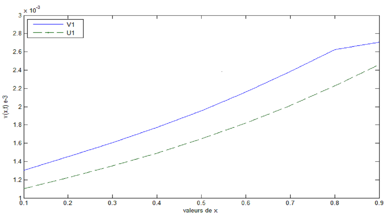
Figure 1.  $\alpha=1.5$, $h_{t}=0.01$

Table 2. $h=0.1$; $h_{t}\mathbf{=}0.001$

$h$ $\ v^{1}(x,t)$ $0.1$ $3.4949e-05$ $0.2$ $3.8624e-05$ $0.3$ $4.2686e-05$ $0.4$ $4.7176e-05$ $0.5$ $5.2137e-05$ $0.6$ $5.7620e-05$ $0.7$ $6.3680e-05$ $0.8$ $7.0378e-05$ $0.9$ $7.7802e-05$ $u^{1}(x,t)$ $4.1175e-05$ $4.5515e-05$ $5.0301e-05$ $5.5590e-05$ $6.1435e-05$ $6.7895e-05$ $7.5034e-05$ $8.2923e-05$ $9.1415e-05$ $\ \ \ \ \ \ \ \mathbf{A.E}$ $6.23e-06$ $6.89e-06$ $7.61e-06$ $8.41e-06$ $9.30e-06$ $1.03e-05$ $1.14e-05$ $1.25e-05$ $1.36e-05$

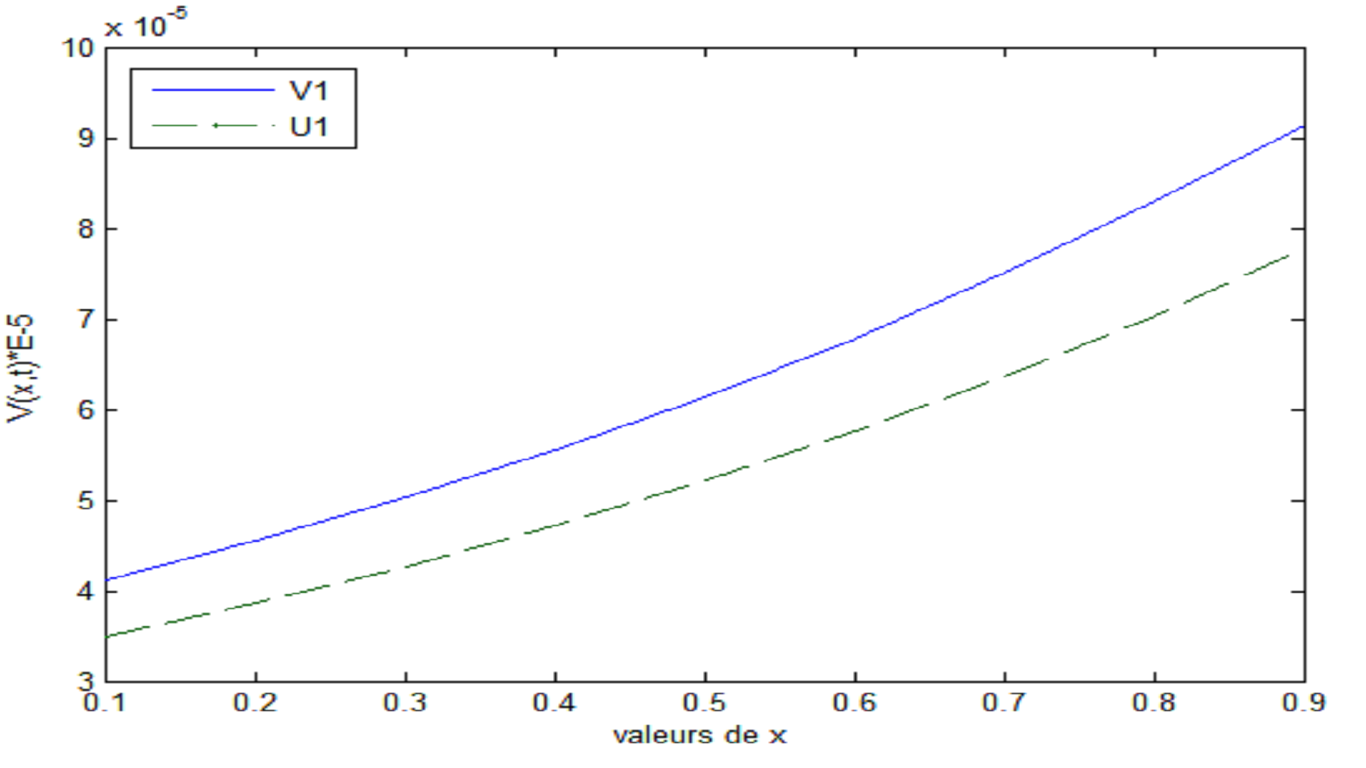
Figure 2.  $\alpha=1.5$, $h_{t}=0.001$

Table 3. $h=0.1;$ $h_{t}\mathbf{=0.0001}$

$h$ $\ v^{1}(x,t)$ $0.1$ $1.1052e-06$ $0.2$ $1.2214e-06$ $0.3$ $1.3499e-06$ $0.4$ $1.4918e-06$ $0.5$ $1.6487e-06$ $0.6$ $1.8221e-06$ $0.7$ $2.0138e-06$ $0.8$ $2.2255e-06$ $0.9$ $2.4596e-06$ $u^{1}(x,t)$ $1.3020e-06$ $1.4389e-06$ $1.5903e-06$ $1.7575e-06$ $1.9424e-06$ $2.1466e-06$ $2.3724e-06$ $2.6219e-06$ $2.8974e-06$ $\ \mathbf{A.E}$ $1e-07$ $2e-07$ $2e-07$ $2e-07$ $2e-07$ $3e-07$ $3e-07$ $3e-07$ $4e-07$

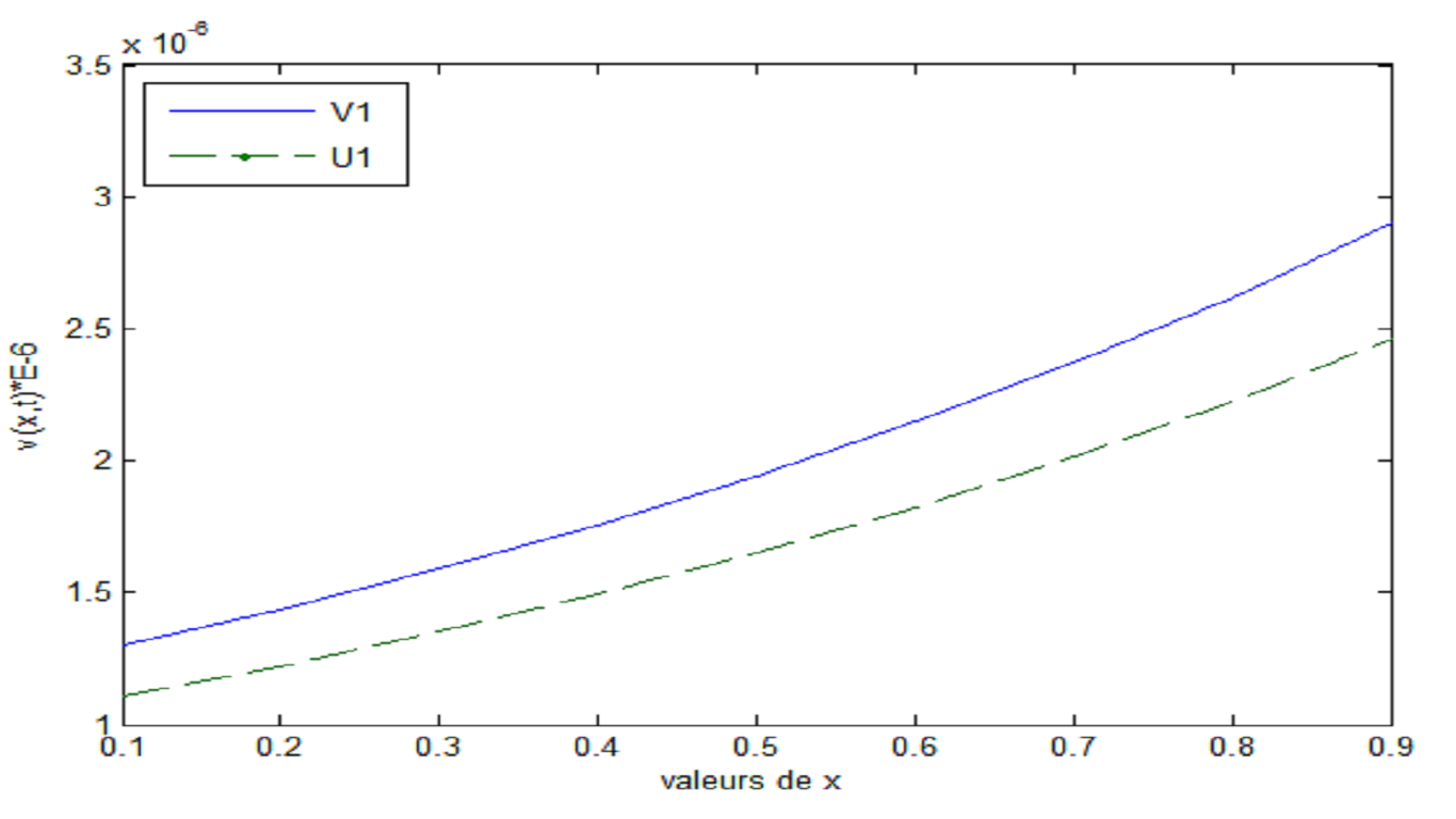
Figure 3.  $\alpha=1.5$, $h_{t}=0.0001$

We see in Figures 1, 2 and 3 that the absolute errors(A.E.) decreases when the step $h_{t}$ takes small values very close to zero. that is, for $h_{t}=0.01$, $h_{t}=0.001$, $h_{t}=0.0001$ A.E decreases towards zero and the approximate solution tends towards the exact solution with convergence order of $O(h+h_{t}).$

For $k=1$  $\left(\text{second iteration}\right)$

Table 4 shows the absolute error for space step $h=0.1$.

$h$ $\ h_{t}=\mathbf{10}^{-2}\ \ \$ $0.1$ $1.84e-03$ $0.2$ $1.74e-03$ $0.3$ $1.62e-03$ $0.4$ $1.49e-03$ $0.5$ $1.33e-03$ $0.6$ $1.17e-03$ $0.7$ $9.82e-04$ $0.8$ $7.40e-04$ $0.9$ $1.26e-04$ $\ \ h_{t}=\mathbf{10}^{-3}$ $5.80e-05$ $5.45e-05$ $5.06e-05$ $4.63e-05$ $4.15e-05$ $3.63e-05$ $3.05e-05$ $2.40e-05$ $1.64e-05$ $\ \ h_{t}=\mathbf{10}^{-5}$ $5.80e-08$ $5.45e-08$ $5.06e-08$ $4.63e-08$ $4.16e-08$ $3.63e-08$ $3.05e-08$ $2.41e-08$ $1.69e-08$

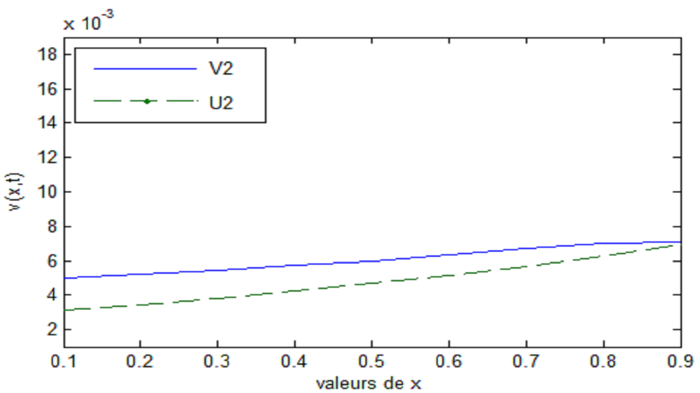
(a) FIGURE 4.    

$h_{t}=\mathbf{10}^{-2}$

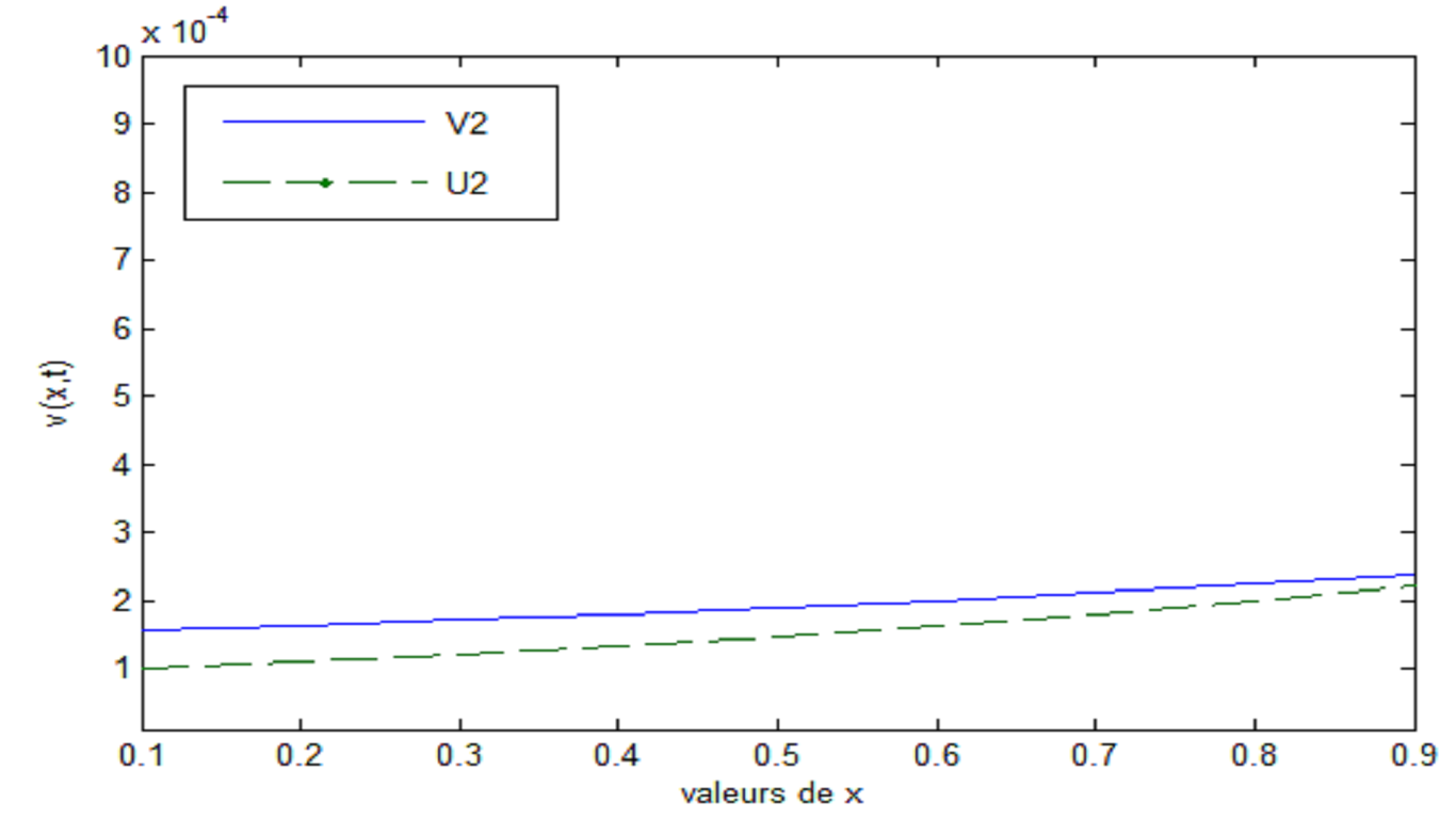
(b) FIGURE 5.     

$h_{t}=\mathbf{10}^{-3}$

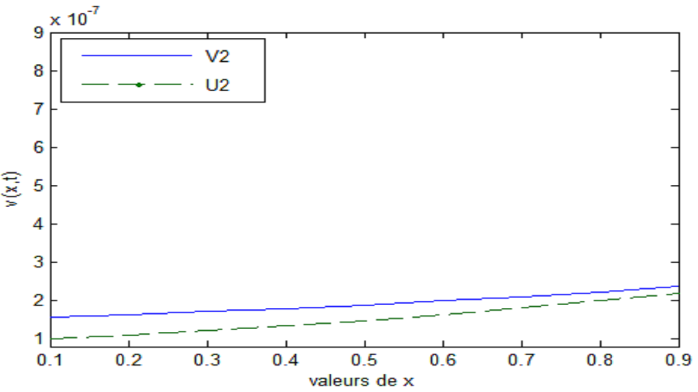
(c) FIGURE 6.      

$h_{t}=\mathbf{10}^{-5}$

Table 4 shows the absolute error decreases to zero and Fig 4,5, and 6 show the approximate solution $u{{}^{2}}$ after two steps $2h_{t}$ tends to the exact solution when $h_{t}$ close to zero, with convergence order $O(h+h_{t}).$

$\overset{\begin{array}[]{cc}&\text{Table 5. The absolute error for }h\mathbf{=0.01};\text{ }h_{t}=\mathbf{10}^{-3}\ \text{\ }\\ &\begin{tabular}[t]{|c|c|c|c|c|c|c|c|c|c|c|}\hline\cr$i=\overline{1,9}$&$\overline{10,18}$&$\overline{19,27}$&$\overline{28,36}$&$\overline{37,45}$&$\overline{46,54}$&$\overline{55,63}$&$\overline{64,72}$&$\overline{73,81}$&$\overline{82,89}$&$\overline{90,99}$\\ \hline\cr 5*10${}^{-6}$&6*10${}^{-6}$&6*10${}^{-6}$&7*10${}^{-6}$&8*10${}^{-6}$&9*10${}^{-6}$&10${}^{-5}$&10${}^{-5}$&10${}^{-5}$&10${}^{-5}$&10${}^{-5}$\\ \hline\cr 5*10${}^{-6}$&6*10${}^{-6}$&7*10${}^{-6}$&7*10${}^{-6}$&8*10${}^{-6}$&9*10${}^{-6}$&10${}^{-5}$&10${}^{-5}$&10${}^{-5}$&10${}^{-5}$&10${}^{-5}$\\ \hline\cr 5*10${}^{-6}$&6*10${}^{-6}$&7*10${}^{-6}$&7*10${}^{-6}$&8*10${}^{-6}$&9*10${}^{-6}$&10${}^{-5}$&10${}^{-5}$&10${}^{-5}$&10${}^{-5}$&10${}^{-5}$\\ \hline\cr 6*10${}^{-6}$&6*10${}^{-6}$&7*10${}^{-6}$&7*10${}^{-6}$&8*10${}^{-6}$&9*10${}^{-6}$&10${}^{-5}$&10${}^{-5}$&10${}^{-5}$&10${}^{-5}$&10${}^{-5}$\\ \hline\cr 6*10${}^{-6}$&6*10${}^{-6}$&7*10${}^{-6}$&7*10${}^{-6}$&8*10${}^{-6}$&9*10${}^{-6}$&10${}^{-5}$&10${}^{-5}$&10${}^{-5}$&10${}^{-5}$&10${}^{-5}$\\ \hline\cr 6*10${}^{-6}$&6*10${}^{-6}$&7*10${}^{-6}$&7*10${}^{-6}$&8*10${}^{-6}$&9*10${}^{-6}$&10${}^{-5}$&10${}^{-5}$&10${}^{-5}$&10${}^{-5}$&10${}^{-5}$\\ \hline\cr 6*10${}^{-6}$&6*10${}^{-6}$&7*10${}^{-6}$&8*10${}^{-6}$&8*10${}^{-6}$&9*10${}^{-6}$&10${}^{-5}$&10${}^{-5}$&10${}^{-5}$&10${}^{-5}$&10${}^{-5}$\\ \hline\cr 6*10${}^{-6}$&6*10${}^{-6}$&7*10${}^{-6}$&8*10${}^{-6}$&8*10${}^{-6}$&9*10${}^{-6}$&10${}^{-5}$&10${}^{-5}$&10${}^{-5}$&10${}^{-5}$&10${}^{-5}$\\ \hline\cr 6*10${}^{-6}$&6*10${}^{-6}$&7*10${}^{-6}$&8*10${}^{-6}$&8*10${}^{-6}$&9*10${}^{-6}$&10${}^{-5}$&10${}^{-5}$&10${}^{-5}$&10${}^{-5}$&10${}^{-5}$\\ \hline\cr\end{tabular}\end{array}}{}$

FIGURE 7, $\alpha=1.5$, $h_{t}=10^{-3}$

$\vskip 12.0pt plus 4.0pt minus 4.0pt\overset{\begin{array}[]{ll}&\text{Table 6. The absolute error for }h=0.01;\text{ }h_{t}\mathbf{=10}^{-5}\ \text{\ }\\ \vspace{0.5in}&\begin{tabular}[t]{|c|c|c|c|c|c|c|c|c|c|c|}\hline\cr$i=\overline{1,9}$&$\overline{10,18}$&$\overline{19,27}$&$\overline{28,36}$&$\overline{37,45}$&$\overline{46,54}$&$\overline{55,63}$&$\overline{64,72}$&$\overline{73,81}$&$\overline{82,89}$&$\overline{90,99}$\\ \hline\cr 5*10${}^{-9}$&6*10${}^{-9}$&6*10${}^{-9}$&7*10${}^{-9}$&8*10${}^{-9}$&8*10${}^{-9}$&9*10${}^{-9}$&10${}^{-8}$&10${}^{-8}$&10${}^{-8}$&10${}^{-8}$\\ \hline\cr 5*10${}^{-9}$&6*10${}^{-9}$&6*10${}^{-9}$&7*10${}^{-9}$&8*10${}^{-9}$&9*10${}^{-9}$&9*10${}^{-9}$&10${}^{-8}$&10${}^{-8}$&10${}^{-8}$&10${}^{-8}$\\ \hline\cr 5*10${}^{-9}$&6*10${}^{-9}$&6*10${}^{-9}$&7*10${}^{-9}$&8*10${}^{-9}$&9*10${}^{-9}$&9*10${}^{-9}$&10${}^{-8}$&10${}^{-8}$&10${}^{-8}$&10${}^{-8}$\\ \hline\cr 5*10${}^{-9}$&6*10${}^{-9}$&7*10${}^{-9}$&7*10${}^{-9}$&8*10${}^{-9}$&9*10${}^{-9}$&10${}^{-9}$&10${}^{-8}$&10${}^{-8}$&10${}^{-8}$&10${}^{-8}$\\ \hline\cr 5*10${}^{-9}$&6*10${}^{-9}$&7*10${}^{-9}$&7*10${}^{-9}$&8*10${}^{-9}$&9*10${}^{-9}$&10${}^{-9}$&10${}^{-8}$&10${}^{-8}$&10${}^{-8}$&10${}^{-8}$\\ \hline\cr 5*10${}^{-9}$&6*10${}^{-9}$&7*10${}^{-9}$&7*10${}^{-9}$&8*10${}^{-9}$&9*10${}^{-9}$&10${}^{-9}$&10${}^{-8}$&10${}^{-8}$&10${}^{-8}$&10${}^{-8}$\\ \hline\cr 6*10${}^{-9}$&6*10${}^{-9}$&7*10${}^{-9}$&7*10${}^{-9}$&8*10${}^{-9}$&9*10${}^{-9}$&10${}^{-9}$&10${}^{-8}$&10${}^{-8}$&10${}^{-8}$&10${}^{-8}$\\ \hline\cr 6*10${}^{-9}$&6*10${}^{-9}$&7*10${}^{-9}$&7*10${}^{-9}$&8*10${}^{-9}$&9*10${}^{-9}$&10${}^{-9}$&10${}^{-8}$&10${}^{-8}$&10${}^{-8}$&10${}^{-8}$\\ \hline\cr 6*10${}^{-9}$&6*10${}^{-9}$&7*10${}^{-9}$&8*10${}^{-9}$&8*10${}^{-9}$&9*10${}^{-9}$&10${}^{-9}$&10${}^{-8}$&10${}^{-8}$&10${}^{-8}$&10${}^{-8}$\\ \hline\cr\end{tabular}\end{array}}{}$

FIGURE 8  $\alpha=1.5$, $h_{t}=10^{-5}$

From tables 5, 6 and Fig 7, 8 with space step $h=\mathbf{0.01},$ we see that the approximate solution $u{{}^{1}}$ tends to the exact solution $v{{}^{1}}$ when the step $h_{t}$ $(h_{t}=10^{-3},h_{t}=10^{-5})$ takes values close to zero,with convergence order $O(h+h_{t}).$

Example 17.

We take: $\alpha=\frac{3}{2},\quad a(x,t)=-x^{2}-t,\quad b(x,t)=x-t$,  $c(x)=x+2t,\quad\displaystyle g(x,t)=(4\sqrt{t}+(t+1)^{2}(x^{2}+2t)e^{x},$ $\Phi(x)=e^{x};\quad$, $\psi(x)=2e^{x},\quad\mu(t)=(t+1)^{2},\quad E(t)=(t+1)^{2}.$

The exact analytical solution of this problem is given by $v(x,t)=(t+1)^{2}e^{x}.$

The tables 7, 8 and 9 show the values of the absolute error.

$\begin{array}[]{c}\text{Table 7.\ }h\text{ }\mathbf{=0.1},\text{ }h_{t}=\mathbf{10}^{-2}\\ \begin{tabular}[]{|l|l|}\hline\cr$h$&\ \ \ \ $\mathbf{A.E}$\\ \hline\cr$0.1$&\vrule\lx@intercol\hfil$6.72e-04$\hfil\lx@intercol\vrule\lx@intercol \\ \hline\cr$0.2$&\vrule\lx@intercol\hfil$2.47e-03$\hfil\lx@intercol\vrule\lx@intercol \\ \hline\cr$0.3$&\vrule\lx@intercol\hfil$2.44e-03$\hfil\lx@intercol\vrule\lx@intercol \\ \hline\cr$0.4$&\vrule\lx@intercol\hfil$2.41e-03$\hfil\lx@intercol\vrule\lx@intercol \\ \hline\cr$0.5$&\vrule\lx@intercol\hfil$2.39e-03$\hfil\lx@intercol\vrule\lx@intercol \\ \hline\cr$0.6$&\vrule\lx@intercol\hfil$2.38e-03$\hfil\lx@intercol\vrule\lx@intercol \\ \hline\cr$0.7$&\vrule\lx@intercol\hfil$1.84e-03$\hfil\lx@intercol\vrule\lx@intercol \\ \hline\cr$0.8$&\vrule\lx@intercol\hfil$1.40e-02$\hfil\lx@intercol\vrule\lx@intercol \\ \hline\cr$0.9$&\vrule\lx@intercol\hfil$2.06e-01$\hfil\lx@intercol\vrule\lx@intercol \\ \hline\cr\end{tabular}\end{array}$

FIGURE 9.  $\alpha=1.5$, $h_{t}=10^{-4}$

$\begin{array}[]{c}\text{Table 8. }h=\mathbf{0.1},\text{ }h_{t}=\mathbf{10}^{-3}\\ \begin{tabular}[]{|l|l|}\hline\cr$h$&$\ \ \ \ \ \ \mathbf{A.E}$\\ \hline\cr$0.1$&\vrule\lx@intercol\hfil$1.22e-05$\hfil\lx@intercol\vrule\lx@intercol \\ \hline\cr$0.2$&\vrule\lx@intercol\hfil$4.28e-05$\hfil\lx@intercol\vrule\lx@intercol \\ \hline\cr$0.3$&\vrule\lx@intercol\hfil$4.24e-05$\hfil\lx@intercol\vrule\lx@intercol \\ \hline\cr$0.4$&\vrule\lx@intercol\hfil$4.20e-05$\hfil\lx@intercol\vrule\lx@intercol \\ \hline\cr$0.5$&\vrule\lx@intercol\hfil$4.15e-05$\hfil\lx@intercol\vrule\lx@intercol \\ \hline\cr$0.6$&\vrule\lx@intercol\hfil$4.10e-05$\hfil\lx@intercol\vrule\lx@intercol \\ \hline\cr$0.7$&\vrule\lx@intercol\hfil$4.03e-05$\hfil\lx@intercol\vrule\lx@intercol \\ \hline\cr$0.8$&\vrule\lx@intercol\hfil$4.83e-05$\hfil\lx@intercol\vrule\lx@intercol \\ \hline\cr$0.9$&\vrule\lx@intercol\hfil$5.48e-03$\hfil\lx@intercol\vrule\lx@intercol \\ \hline\cr\end{tabular}\end{array}$

FIGURE 10  $\alpha=1.5$, $h_{t}=10^{-5}$

$\begin{array}[]{c}\text{Table 9. }h=0.1,\text{ }h_{t}=\mathbf{10}^{-4}\\ \lx@intercol\text{ \ \ \ \ \ \ }\begin{tabular}[t]{|r|r|}\hline\cr$h$&$\mathbf{A.E}$\\ \hline\cr$0.1$&$3.75e-07$\\ \hline\cr$0.2$&$1.26e-06$\\ \hline\cr$0.3$&$1.24e-06$\\ \hline\cr$0.4$&$1.25e-06$\\ \hline\cr$0.5$&$1.23e-06$\\ \hline\cr$0.6$&$1.22e-06$\\ \hline\cr$0.7$&$1.20e-06$\\ \hline\cr$0.8$&$1.19e-06$\\ \hline\cr$0.9$&$1.72e-04$\\ \hline\cr\end{tabular}\hfil\lx@intercol\end{array}$

FIGURE 11  $\alpha=1.5$, $h_{t}=10^{-5}$

In this example we see again for space step $h=0.1$ the absolute error tends to zero, when the time step $h_{t}$ $(\mathbf{10}^{-2},$ $\mathbf{10}^{-3},$ $\mathbf{10}^{-4})$ takes a value close to zero, with convergence order $O(h+h_{t}).$

For $h=\mathbf{0.01,}$ $\alpha=1.5$

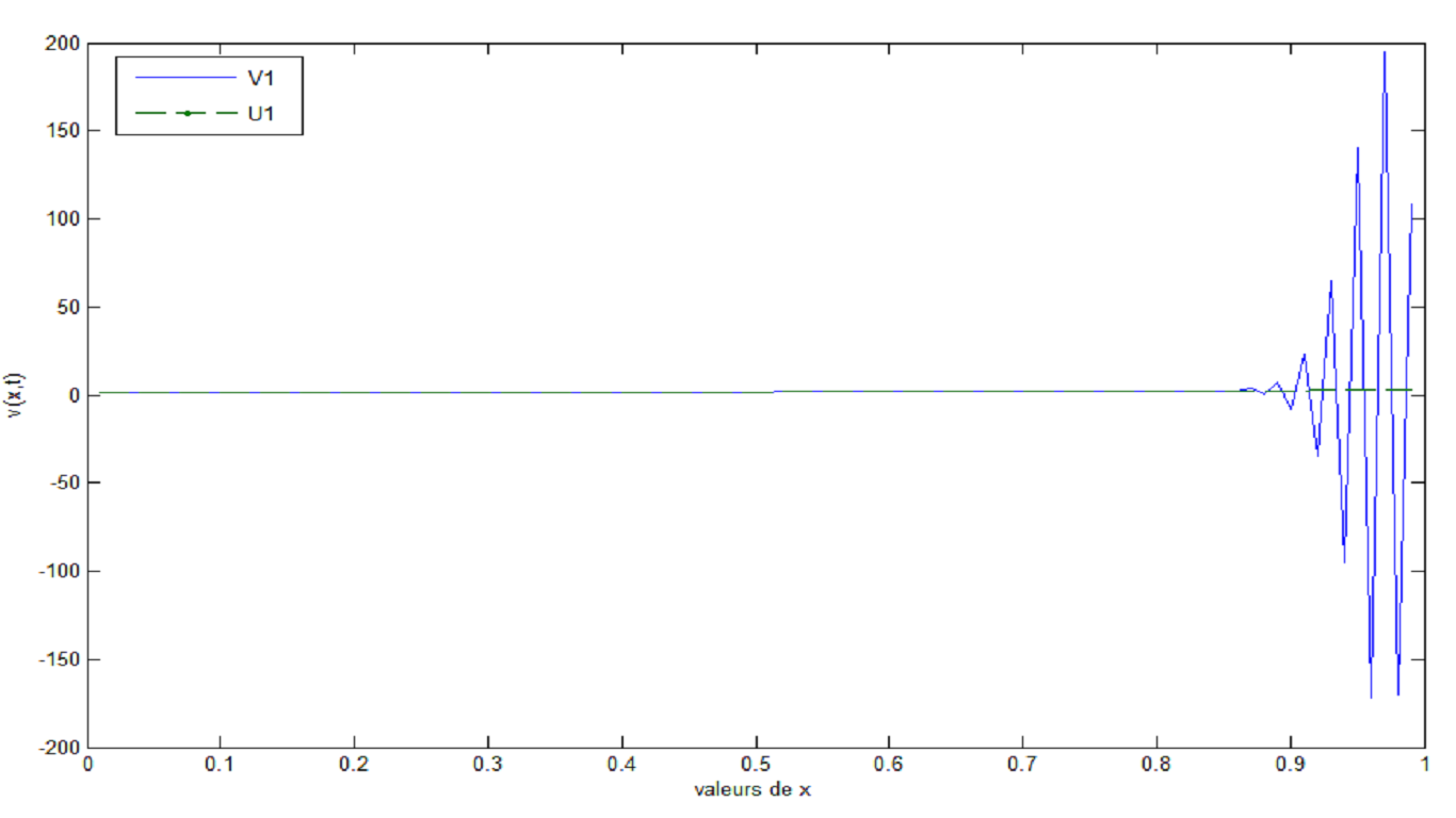
(a) FIGURE 12.    

$h_{t}=\mathbf{10}^{-2}$

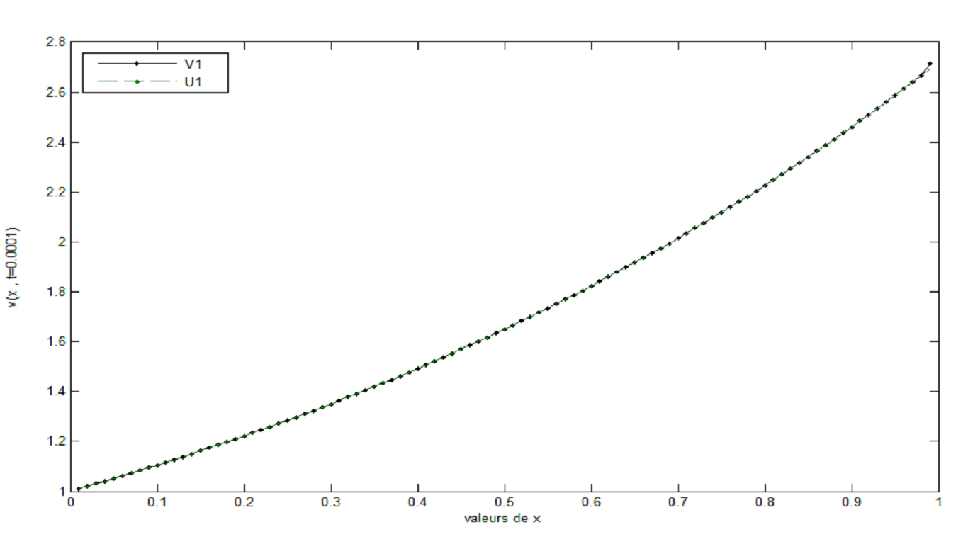
(b) FIGURE 13.     

$h_{t}=\mathbf{10}^{-3}$

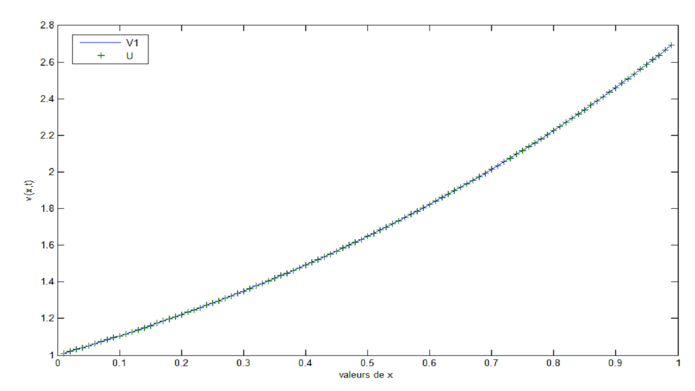
(c) FIGURE 14.      

$h_{t}=\mathbf{10}^{-5}$

Fig. 12      $h_{t}=0.001$              Fig. 13      $h_{t}=0.0001$                Fig. 14    $h_{t}=0.00001$

The Fig.12 ,13 and 14 show where the space step is fixed at $h=0.01$ and the time step $h_{t}$ decreases towards zero $(h_{t}=0.001$, $h_{t}=0.0001,$ $h_{t}=0.00001),$ the approximate solution $u{{}^{1}}$ tends to the exact solution $v{{}^{1}}$, in the case where $h_{t}=0.00001$ we see that the two curves of $u{{}^{1}}$ and $v{{}^{1}}$ are almost identical.

Table $10$ shows the error norm $\left\|E^{k}\right\|_{\infty}$ for defferent value of $\alpha$ defined by

$$\left\|E^{k}\right\|_{\infty}=\mathop{\mathrm{M}ax}_{\text{ }1\text{ }\leq\text{ }i\text{ }\leq\text{ }N-1}\mathop{\displaystyle\sum}\limits_{i=1}^{N-1}\left|e_{i}\right|,\text{ where }E^{k}=V\text{ }^{k}-U\text{ }^{k}=\left(e_{1}^{k},...,e_{N-1}^{k}\right)^{T}$$

$$\text{Table }10\text{ },\text{ }h=0.1$$

$\ \ \ \ \ \ \ \ \ \ \ \ \ \ \ h_{t}$	$\ \ 10^{-3}$  $\ \ \ 10^{-5}$ $10^{-7}$
$\left\|E^{1}\right\|_{\infty}$ for $\alpha=1.2$ $\alpha=1.4$ $\alpha=1.6$ $\alpha=1.8$ $\alpha=1.9$	$\ \ \ 9.5736e\ast 10^{-4}$ $1.3196\ast 10^{-6}\$ $5.2768\ast 10^{-9}\$ $\ 1.1294\ast 10^{-4}$ $\ 1.2671\ast 10^{-7}$ $2.0154\ast 10^{-10}$ $2.3162\ast 10^{-5}$ $1.2692\ast 10^{-8}$ $7.9794\ast 10^{-12}$ $1.53\ast 10^{-4}$ $1.4449\ast 10^{-9}$ $3.4062\ast 10^{-13}$ $4.7963\ast 10^{-6}$ $6.2306\ast 10^{-10}$ $8.6153\ast 10^{-14}$

We see in the table 10, for the space step $h=0.1,$ and for the defferent values of $\alpha,$ the error norm tends to zeros when the time step $h_{t}$ takes values close to zeros, with convergence order $O(h+h_{t}).$

Conclusion

In this paper, we study a problem with fractional derivatives with boundary conditions of integral types. The study concerns a Caputo-type advection-diffusion equation where the fractional order derivative $\alpha$ with respect to time with $1<\alpha<2$. The existence and uniqueness are proven by the method of energy inequalities. The numerical study of this problem based on the finite difference method. Applications on certain examples clearly show that the numerical results obtained are very satisfactory, where we see the approximate solution $u$ tends to the exact solution $v$ for the defferent value of $\alpha.$

References

- [1] A Akilandeeswariy, K Ba achandran, N Annapoorani; Solvability of hyperbolic fractional partial Differantial Eequations, Journal of Applied Analysisand Computation, 7(4), (2017), 1570–1585.
- [2] A. Anguraj, P. Karthikeyan; Existence of solutions for fractional semilinear evolution boundary value problem, Commun. Appl. Anal. 14 (2010), 505–514.
- [3] A. A. Alikhanov, On the stability and convergence of nonlocal difference schemes, Differ. Equ. 46(7), (2010), 949–961.
- [4] A. A. Kilbas, H. M. Srivastava, J. J. Trujillo; Theory and Applications of Fractional Differential Equations, Elsevier, Amsterdam, 2006.
- [5] A. A. Alikhanov, Boundary value problems for the diffusion equation of the variable order in differential and difference settings, Appl. Math. Comput. 219 (2012), no. 8, 3938–3946.
- [6] A. A. Alikhanov, A new difference scheme for the time fractional diffusion equation, J. Comput. Phys. 280 (2015), 424–438.
- [7] A. A. Alikhanov, Stability and convergence of difference schemes for boundary value problems for the fractional-order diffusion equation, Comput. Math. Math. Phys. 56 (2016), no. 4, 561–575.
- [8] A. Bouziani, On the weak solution of three-point boundary value for problem for a class of parabolic equations with energy specification, Appl. Anal., 2003:576–589.
- [9] E. R. Kaufmann, E. Mboumi; Positive solutions of a boundary value problem for a nonlinear. fractional differential equation, Electron. J. Qual. Theory Differ. Equ. 3 (2007) 1–11.
- [10] F. Mainardi, Fractional diffusive waves in viscoelastic solids, Nonlinear Waves in Solids,1995, 93–97.
- [11] J. H. He; Approximate analytical solution for seepage flow with fractional derivatives in porous media. Comput Methods Appl Mech Eng. 167, (1998), 57–68.
- [12] Jesus Martin-Vaquero, Ahcene Merad existence,uniqueness and numerical solution of a fractional PDE with integral conditions, Nonlinear Analysis: Modelling and control, 2019, Vol.24, No.3,368–386.
- [13] K. M. Furati, N. Tatar; An existence result for a nonlocal fractional differential problem, J. Fract. Calc. 26 (2004), 43–51.
- [14] L. C. Evans, Partial Differential Equations, American Mathematical Society, Providence, 1998.
- [15] Meerschaert, M. M.; Tadjeran, C. Finite difference approximations for fractional advection–dispersion flow equations. J. Comput. Appl. Math. 2004, 172, 65–77.
- [16] M. Benchohra, J. R. Graef, S. Hamani, Existence results for boundary value problems with nonlinear fractional differential equations, Appl. Anal. 87 (2008), 851–863.
- [17] M. El-Mikkawy, A. Karawia, Inversion of general tridiagonal matrices Applied Mathematics Letters 19 (2006), 712–720.
- [18] N. J. Ford, J. Xiao, Y. Yan, A Finite element method for time fractional partial differential equations. Fractional Calculus and Applied Analysis, 14(3) (2011), 454–474.
- [19] Nicolas Bertrand, electrical characterization of physicochemical phenomena and fractional modeling of supercapacitors with activated carbon-based electrodes, PhD thesis in electronics, 2011, University Bordeaux.
- [20] Octavian Enacheanu, Fractal modeling of electrical networks, doctoral thesis p. 47-53, October 2008, Joseph Fourier University.
- [21] Podlubny, I. Fractional Differential Equations; Academic Press: San Diego, CA, USA, 1999.
- [22] R. Metzler, J. Klafter; The random walk’s guide to anomalous diffusion: a fractional dynamics approach. Phys Rep., 339, 1–77 (2000).
- [23] R. P. Agarwal, M. Benchohra, S. Hamani, Boundary value problems for fractional differential equations, Adv. Stud. Contemp. Math. 16 (2008) 181–196.
- [24] R. Metzler and J. Klafter, The random walk’s guide to anomalous diffusion: a fractional dynamics approach, Phys. Rep., 339 (2000), 1–77.
- [25] S. M. Momani, S .B. Hadid, Z. M. Alawenh; Some analytical properties of solutions of defferential equations of non-integer order, Int. J. Math. Math. Sci. 13 (2004) 697–701.
- [26] S. Shen and F. Liu, Error analysis of an explicit finite difference approximation for the space fractional difusion, ANZIAM J.,46 (E), (2005).
- [27] S. Mesloub, Existence and uniqueness results for a fractional two-times evolution problem with constraints of purely integral type, Mathematical Methods in the Applied Sciences, 2016, 39(6), 1558–1567.
- [28] T-E. Oussaeif, A Bouziani; Existence and uniqueness of solutions to parabolic fractional differential equations with integral conditions, Electronic Journal of Differential Equations, Vol. 2014 (2014), no. 179, 1–10.
- [29] V. Daftardar-Gejji, H. Jafari; Boundary value problems for fractional diffusion-wave equation, Aust. J. Math. Anal. Appl. 3 (2006) 1–8.
- [30] V. Feliu, B. M. Vinagre, I. Petras and I. Podlubny, Y. Chen, Non-integer derivatives in automatic control and signal processing: some challenges, October 2001, Bordeaux.
- [31] X. J. Li, C. J. Xu; Existence and uniqueness of the weak solution of the space-time fractional diffusion equation and a spectral method approximation, Communications in Computational Physics, vol. 8, no. 5, 1016–1051, 2010.
- [32] Y. Luchko, Initial-boundary-value problems for the one-dimensional time-fractional diffusion equation, Fract Calc. Appl.Anal. 15 (2012), no. 1, 141–160.
- [33] W. Smit and H. de Vries, Rheological models containing fractional derivatives. Rheologica Acta, vol. 9. 1970. 525–534.
- [34] W. A. Day, A decreasing property of solutions of parabolic equations with applications to thermoelasticity, Quart. Appl.Math., Vol. 40, No. 4 (1983), 319–330.
- [35] W. A. Day, Parabolic equations and thermodynamics, Quart. Appl. Math., Vol. 50, No. 3 (1992), 523–533.