Few-shot Network Anomaly Detection via Cross-network Meta-learning

Abstract.

Network anomaly detection aims to find network elements (e.g., nodes, edges, subgraphs) with significantly different behaviors from the vast majority. It has a profound impact in a variety of applications ranging from finance, healthcare to social network analysis. Due to the unbearable labeling cost, existing methods are predominately developed in an unsupervised manner. Nonetheless, the anomalies they identify may turn out to be data noises or uninteresting data instances due to the lack of prior knowledge on the anomalies of interest. Hence, it is critical to investigate and develop few-shot learning for network anomaly detection. In real-world scenarios, few labeled anomalies are also easy to be accessed on similar networks from the same domain as of the target network, while most of the existing works omit to leverage them and merely focus on a single network. Taking advantage of this potential, in this work, we tackle the problem of few-shot network anomaly detection by (1) proposing a new family of graph neural networks – Graph Deviation Networks (GDN) that can leverage a small number of labeled anomalies for enforcing statistically significant deviations between abnormal and normal nodes on a network; (2) equipping the proposed GDN with a new cross-network meta-learning algorithm to realize few-shot network anomaly detection by transferring meta-knowledge from multiple auxiliary networks. Extensive evaluations demonstrate the efficacy of the proposed approach on few-shot or even one-shot network anomaly detection.

1. Introduction

Network-structured data, ranging from social networks (Zafarani et al., 2014) to team collaboration networks (Zhou et al., 2019a), from citation networks (Tang et al., 2008) to molecular graphs (You et al., 2018), has been widely used in modeling a myriad of real-world systems. Nonetheless, real-world networks are commonly contaminated with a small portion of nodes, namely, anomalies, whose patterns significantly deviate from the vast majority of nodes (Ding et al., 2019a, 2020a; Zhou et al., 2018). For instance, in a citation network that represents citation relations between papers, there are some research papers with a few spurious references (i.e., edges) which do not comply with the content of the papers (Bandyopadhyay et al., 2019); In a social network that represents friendship of users, there may exist camouflaged users who randomly follow different users, rendering properties like homophily not applicable to this type of relationships (Dou et al., 2020). As the existence of even few abnormal instances could cause extremely detrimental effects, the problem of network anomaly detection has received much attention in industry and academy alike.

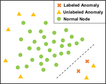
(a) Latent Representation Space

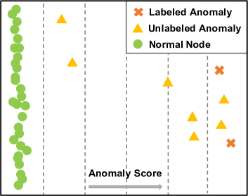
(b) Anomaly Score Space

Figure 1. Since anomalies usually have distinct patterns, (a) existing methods may easily fail to distinguish them from normal nodes in the latent representation space with only few labeled anomalies, (b) while they can be well separated in an anomaly score space by enforcing statistically significant deviations between abnormal and normal nodes.

Due to the fact that labeling anomalies is highly labor-intensive and takes specialized domain-knowledge, existing methods are predominately developed in an unsupervised manner. As a prevailing paradigm, people try to measure the abnormality of nodes with the reconstruction errors of autoencoder-based models (Ding et al., 2019b; Li et al., 2019a) or the residuals of matrix factorization-based methods (Tong and Lin, 2011; Li et al., 2017; Bandyopadhyay et al., 2019). However, the anomalies they identify may turn out to be data noises or uninteresting data instances due to the lack of prior knowledge on the anomalies of interest. A potential solution to this problem is to leverage limited or few labeled anomalies as the prior knowledge to learn anomaly-informed models, since it is relatively low-cost in real-world scenarios – a small set of labeled anomalies could be either from a deployed detection system or be provided by user feedback. In the meantime, such valuable knowledge is usually scattered among other networks within the same domain of the target one, which could be further exploited for distilling supervised signal. For example, LinkedIn and Indeed have similar social networks that represent user friendship in the job-search domain; ACM and DBLP can be treated as citation networks that share similar citation relations in the computer science domain. According to previous studies (Tang et al., 2020; Zhou et al., 2020; Zhou et al., 2019b), because of the similarity of topological structure and nodal attributes, it is feasible to transfer valuable knowledge from source network(s) to the target network so that the performance on the target one is elevated. As such, in this work we propose to investigate the novel problem of few-shot network anomaly detection under the cross-network setting.

Nonetheless, solving this under-explored problem remains non-trivial, mainly owing to the following reasons: (1) From the micro (intra-network) view, since we only have limited knowledge of anomalies, it is hard to precisely characterize the abnormal patterns. If we directly adopt existing semi-supervised (Wang et al., 2019) or PU (Wu et al., 2019a) learning techniques, those methods often fall short in achieving satisfactory results as they might still require a relatively large percentage of positive examples (Pang et al., 2019). To handle such incomplete supervision challenge (Zhang et al., 2019) as illustrated in Figure 1(a), instead of focusing on abnormal nodes, how to leverage labeled anomalies as few as possible to learn a high-level abstraction of normal patterns is necessary to be explored; (2) From the macro (inter-network) view, though networks in the same domain might share similar characteristics in general, anomalies exist in different networks may be from very different manifolds. Previous studies on cross-network learning (Wu et al., 2020; Shen et al., 2020) mostly focus on transferring the knowledge only from a single network, which may cause unstable results and the risk of negative transfer. As learning from multiple networks could provide more comprehensive knowledge about the characteristics of anomalies, a cross-network learning algorithm that is capable of adapting the knowledge is highly desirable.

To address the aforementioned challenges, in this work we first design a new GNN architecture, namely Graph Deviation Networks (GDN), to enable network anomaly detection with limited labeled data. Specifically, given an arbitrary network, GDN first uses a GNN-backboned anomaly score learner to assign each node with an anomaly score, and then defines the mean of the anomaly scores based on a prior probability to serve as a reference score for guiding the subsequent anomaly score learning. By leveraging a deviation loss (Pang et al., 2019), GDN is able to enforce statistically significant deviations of the anomaly scores of anomalies from that of normal nodes in the anomaly score space (as shown in Figure 1(b)). To further transfer this ability from multiple networks to the target one, we propose a cross-network meta-learning algorithm to learn a well-generalized initialization of GDN from multiple few-shot network anomaly detection tasks. The seamlessly integrated framework Meta-GDN is capable of extracting comprehensive meta-knowledge for detecting anomalies across multiple networks, which largely alleviates the limitations of transferring from a single network. Subsequently, the initialization can be easily adapted to a target network via fine-tuning with few or even one labeled anomaly, improving the anomaly detection performance on the target network to a large extent. To summarize, our main contributions is three-fold:

• Problem: To the best of knowledge, we are the first to investigate the novel problem of few-shot network anomaly detection. Remarkably, we propose to solve this problem by transferring the knowledge across multiple networks.

• Algorithms: We propose a principled framework Meta-GDN, which integrates a new family of graph neural networks (i.e., GDN) and cross-network meta-learning to detect anomalies with few labeled instances.

• Evaluations: We perform extensive experiments to corroborate the effectiveness of our approach. The experimental results demonstrate the superior performance of Meta-GNN over the state-of-the-art methods on network anomaly detection.

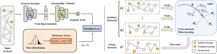
Figure 2. (Left) The model architecture of Graph Deviation Networks (GDN) for network anomaly detection with limited labeled data. (Right) The illustration of the overall framework Meta-GDN. Meta-GDN is trained across multiple auxiliary networks and can be well adapted to the target network with few-shot labeled data. Figure best viewed in color.

2. Related Work

In this section, we review the related work in terms of (1) network anomaly detection; and (2) graph neural networks.

2.1. Network Anomaly Detection

Network anomaly detection methods have a specific focus on the network structured data. Previous research mostly study the problem of anomaly detection on plain networks. As network structure is the only available information modality in a plain network, this category of anomaly detection methods try to exploit the network structure information to spot anomalies from different perspectives (Akoglu et al., 2015; Xu et al., 2007). For instance, SCAN (Xu et al., 2007) is one of the first methods that target to find structural anomalies in networks. In recent days, attributed networks have been widely used to model a wide range of complex systems due to their superior capacity for handling data heterogeneity. In addition to the observed node-to-node interactions, attributed networks also encode a rich set of features for each node. Therefore, anomaly detection on attributed networks has drawn increasing research attention in the community, and various methods have been proposed  (Müller et al., 2013; Sánchez et al., 2014). Among them, ConOut (Müller et al., 2013) identifies the local context for each node and performs anomaly ranking within the local context. More recently, researchers also propose to solve the problem of network anomaly detection using graph neural networks due to its strong modeling power. DOMINANT (Ding et al., 2019b) achieves superior performance over other shallow methods by building a deep autoencoder architecture on top of the graph convolutional networks. Semi-GNN (Wang et al., 2019) is a semi-supervised graph neural model which adopts hierarchical attention to model the multi-view graph for fraud detection. GAS (Li et al., 2019b) is a GCN-based large-scale anti-spam method for detecting spam advertisements. Zhao et al. propose a novel loss function to train GNNs for anomaly-detectable node representations  (Zhao et al., 2020). Apart from the aforementioned methods, our approach focus on detecting anomalies on a target network with few labels by learning from multiple auxiliary networks.

2.2. Graph Neural Networks

Graph neural networks (Cao et al., 2016; Kipf and Welling, 2017; Veličković et al., 2018; Hamilton et al., 2017) have achieved groundbreaking success in transforming the information of a graph into low-dimensional latent representations. Originally inspired by graph spectral theory, spectral-based graph convolutional networks (GCNs) have emerged and demonstrated their efficacy by designing different graph convolutional layers. Among them, The model proposed by Kipf et al. (Kipf and Welling, 2017) has become the most prevailing one by using a linear filter. In addition to spectral-based graph convolution models, spatial-based graph neural networks that follow neighborhoods aggregation schemes also have been extensively investigated. Instead of training individual embeddings for each node, those methods learn a set of aggregator functions to aggregate features from a node’s local neighborhood. GraphSAGE (Hamilton et al., 2017) learns an embedding function that can be generalized to unseen nodes, which enables inductive representation learning on network-structured data. Similarly, Graph Attention Networks (GATs) (Veličković et al., 2018) proposes to learn hidden representations by introducing a self-attention strategy when aggregating neighborhood information of a node. Furthermore, Graph Isomorphism Network (GIN) (Xu et al., 2019) extends the idea of parameterizing universal multiset functions with neural networks, and is proven to be as theoretically powerful as the Weisfeiler-Lehman (WL) graph isomorphism test. To go beyond a single graph and transfer the knowledge across multiple ones, more recently, researchers have explored to integrate GNNs with meta-learning techniques (Zügner and Günnemann, 2019; Tang et al., 2020; Zhou et al., 2020). For instance, PA-GNN (Tang et al., 2020) transfers the robustness from cleaned graphs to the target graph via meta-optimization. Meta-NA (Zhou et al., 2020) is a graph alignment model that learns a unified metric space across multiple graphs, where one can easily link entities across different graphs. However, those efforts cannot be applied to our problem and we are the first to study the problem of few-shot cross-network anomaly detection.

3. Problem Definition

In this section, we formally define the problem of few-shot cross-network anomaly detection. Throughout the paper, we use bold uppercase letters for matrices (e.g., $\mathbf{A}$), bold lowercase letters for vectors (e.g., $\mathbf{u}$), lowercase letters for scalars (e.g., $s$) and calligraphic fonts to denote sets (e.g., $\mathcal{V}$). Notably, in this work we focus on attributed network for a more general purpose. Given an attributed network $\mathbf{G}=(\mathcal{V},\mathcal{E},\mathbf{X})$ where $\mathcal{V}$ is the set of nodes, i.e., $\{v_{1},v_{2},\dots,v_{n}\}$, $\mathcal{E}$ denotes the set of edges, i.e., $\{e_{1},e_{2},\dots,e_{m}\}$. The node attributes are represented by $\mathbf{X}=[\mathbf{x}_{1}^{\mathrm{T}},\mathbf{x}_{2}^{\mathrm{T}},\cdots,\mathbf{x}_{n}^{\mathrm{T}}]\in\mathbb{R}^{n\times d}$ and $\mathbf{x}_{i}$ is the attribute vector for node $v_{i}$. More concretely, we represent the attributed network as $\mathbf{G}=(\mathbf{A},\mathbf{X})$, where $\mathbf{A}=\{0,1\}^{n\times n}$ is an adjacency matrix representing the network structure. Specifically, $\mathbf{A}_{i,j}=1$ indicates that there is an edge between node $v_{i}$ and node $v_{j}$; otherwise, $\mathbf{A}_{i,j}=0$.

Generally speaking, few-shot cross-network anomaly detection aims to maximally improve the detection performance on the target network through transferring very limited supervised knowledge of ground-truth anomalies from the auxiliary network(s). In addition to the target network $\mathbf{G}^{t}$, in this work we assume there exist $P$ auxiliary networks $\mathcal{G}^{s}=\{\mathbf{G}_{1}^{s},\mathbf{G}_{2}^{s},\dots,\mathbf{G}_{P}^{s}\}$ sharing the same or similar domain with $\mathbf{G}^{t}$. For an attributed network, the set of labeled abnormal nodes is denoted as $\mathcal{V}^{L}$ and the set of unlabeled nodes is represented as $\mathcal{V}^{U}$. Note that $\mathcal{V}=\{\mathcal{V}^{L},\mathcal{V}^{U}\}$ and in our problem $|\mathcal{V}^{L}|\ll|\mathcal{V}^{U}|$ since only few-shot labeled data is given. As network anomaly detection is commonly formulated as a ranking problem (Akoglu et al., 2015), we formally define the few-shot cross-network anomaly detection problem as follows:

Problem 1.

Few-shot Cross-network Anomaly Detection

Given::

$P$ auxiliary networks, i.e., $\mathcal{G}^{s}=\{\mathbf{G}_{1}^{s}=(\mathbf{A}_{1}^{s},\mathbf{X}_{1}^{s}),\mathbf{G}_{2}^{s}=(\mathbf{A}_{2}^{s},\mathbf{X}_{2}^{s}),\dots,\mathbf{G}_{P}^{s}=(\mathbf{A}_{P}^{s},\mathbf{X}_{P}^{s})\}$ and a target network $\mathbf{G}^{t}=(\mathbf{A}^{t},\mathbf{X}^{t})$, each of which contains a set of few-shot labeled anomalies (i.e., $\mathcal{V}_{1}^{L},\mathcal{V}_{2}^{L},\dots,\mathcal{V}_{P}^{L}$ and $\mathcal{V}^{L}_{t}$).

Goal::

to learn an anomaly detection model, which is capable of leveraging the knowledge of ground-truth anomalies from the multiple auxiliary networks, i.e., $\{\mathbf{G}_{1}^{s},\mathbf{G}_{2}^{s},\dots,\mathbf{G}_{P}^{s}\}$, to detect abnormal nodes in the target network $\mathbf{G}^{t}$. Ideally, anomalies that are detected should have higher ranking scores than that of the normal nodes.

4. Proposed Approach

In this section, we introduce the details of the proposed framework – Meta-GDN for few-shot network anomaly detection. Specifically, Meta-GDN addresses the discussed challenges with the following two key contributions: (1) Graph Deviation Networks (GDN), a new family of graph neural networks that enable anomaly detection on an arbitrary individual network with limited labeled data; and (2) a cross-network meta-learning algorithm, which empowers GDN to transfer meta-knowledge across multiple auxiliary networks to enable few-shot anomaly detection on the target network. An overview of the proposed Meta-GDN is provided in Figure 2.

4.1. Graph Deviation Networks

To enable anomaly detection on an arbitrary network with few-shot labeled data, we first propose a new family of graph neural networks, called Graph Deviation Network (GDN). In essence, GDN is composed of three key building blocks, including (1) a network encoder for learning node representations; (2) an abnormality valuator for estimating the anomaly score for each node; and (3) a deviation loss for optimizing the model with few-shot labeled anomalies. The details are as follows:

Network Encoder. In order to learn expressive nodes representations from an input network, we first build the network encoder module. Specifically, it is built with multiple GNN layers that encode each node to a low-dimensional latent representation. In general, GNNs follow the neighborhood message-passing mechanism, and compute the node representations by aggregating features from local neighborhoods in an iterative manner. Formally, a generic GNN layer computes the node representations using two key functions:

(1) $$\mathbf{h}_{\mathcal{N}_{i}}^{l} =\textsc{Aggregate}^{l}\Big{(}\{\mathbf{h}_{j}^{l-1}\arrowvert\forall j\in\mathcal{N}_{i}\cup v_{i}\}\Big{)},$$

$$\mathbf{h}_{i}^{l} =\textsc{Transform}^{l}\Big{(}\mathbf{h}_{i}^{l-1},\mathbf{h}_{\mathcal{N}_{i}}^{l}\Big{)},$$

where $\mathbf{h}_{i}^{l}$ is the latent representation of node $v_{i}$ at the $l$-th layer and $\mathcal{N}_{i}$ is the set of first-order neighboring nodes of node $v_{i}$. Notably, $\textsc{Aggregate}(\cdot)$ is an aggregation function that aggregates messages from neighboring nodes and $\textsc{Transform}(\cdot)$ computes the new representation of a node according to its previous-layer representation and the aggregated messages from neighbors.

To capture the long-range node dependencies in the network, we stack multiple GNN layers in the network encoder. Thus, the network encoder can be represented by:

(2) $$\mathbf{H}^{1}=\text{GNN}^{1}(\mathbf{A},\mathbf{X}),$$

$$\dots$$

$$\mathbf{Z}=\text{GNN}^{L}(\mathbf{A},\mathbf{H}^{L-1}),$$

where $\mathbf{Z}$ is the learned node representations from the network encoder. For simplicity, we use a parameterized function $f_{\bm{\theta}_{e}}(\cdot)$ to denote the network encoder with $L$ GNN layers throughout the paper. It is worth noting that the network encoder is compatible with arbitrary GNN-based architecture (Kipf and Welling, 2017; Hamilton et al., 2017; Veličković et al., 2018; Wu et al., 2019b), and here we employ Simple Graph Convolution (SGC) (Wu et al., 2019b) in our implementation.

Abnormality Valuator. Afterwards, the learned node representations from the network encoder will be passed to the abnormality valuator $f_{\bm{\theta}_{s}}(\cdot)$ for further estimating the abnormality of each node. Specifically, the abnormality valuator is built with two feed-forward layers that transform the intermediate node representations to scalar anomaly scores:

(3) $$\mathbf{o}_{i} =\text{ReLU}(\mathbf{W}_{s}\mathbf{z}_{i}+\mathbf{b}_{s}),$$

$$s_{i} =\mathbf{u}^{\mathrm{T}}_{s}\mathbf{o}_{i}+b_{s},$$

where $s_{i}$ is the anomaly score of node $v_{i}$ and $\mathbf{o}_{i}$ is the intermediate output. $\mathbf{W}_{s}$ and $\mathbf{u}_{s}$ are the learnable weight matrix and weight vector, respectively. $\mathbf{b}_{s}$ and $b_{s}$ are corresponding bias terms.

To be more concrete, the whole GDN model $f_{\bm{\theta}}(\cdot)$ can be formally represented as:

(4) $$f_{\bm{\theta}}(\mathbf{A},\mathbf{X})=f_{\bm{\theta}_{s}}(f_{\bm{\theta}_{e}}(\mathbf{A},\mathbf{X})),$$

which directly maps the input network to scalar anomaly scores, and can be trained in an end-to-end fashion.

Deviation Loss. In essence, the objective of GDN is to distinguish normal and abnormal nodes according to the computed anomaly scores with few-shot labels. Here we propose to adopt the deviation loss (Pang et al., 2019) to enforce the model to assign large anomaly scores to those nodes whose characteristics significantly deviate from normal nodes. To guide the model learning, we first define a reference score (i.e., $\mu_{r}$) as the mean value of the anomaly scores of a set of randomly selected normal nodes. It serves as the reference to quantify how much the scores of anomalies deviate from those of normal nodes.

According to previous studies (Pang et al., 2019; Kriegel et al., 2011), Gaussian distribution is commonly a robust choice to fit the abnormality scores for a wide range of datasets. Based on this assumption, we first sample a set of $k$ anomaly scores from the Gaussian prior distribution, i.e., $\mathcal{R}=\{r_{1},r_{2},\dots,r_{k}\}\sim\mathcal{N}(\mu,\sigma^{2})$, each of which denotes the abnormality of a random normal node. The reference score is computed as the mean value of all the sampled scores:

(5) $$\mu_{r}=\frac{1}{k}\sum_{i=1}^{k}r_{i}.$$

With the reference score $\mu_{r}$, the deviation between the anomaly score of node $v_{i}$ and the reference score can be defined in the form of standard score:

(6) $$\text{dev}(v_{i})=\frac{s_{i}-\mu_{r}}{\sigma_{r}},$$

where $\sigma_{r}$ is the standard deviation of the set of sampled anomaly scores $\mathcal{R}=\{r_{1},\dots,r_{k}\}$. Then the final objective function can be derived from the contrastive loss (Hadsell et al., 2006) by replacing the distance function with the deviation in Eq. (6):

(7) $$\mathcal{L}=(1-y_{i})\cdot|\text{dev}(v_{i})|+y_{i}\cdot\text{max}(0,m-\text{dev}(v_{i})),$$

where $y_{i}$ is the ground-truth label of input node $v_{i}$. If node $v_{i}$ is an abnormal node, $y_{i}=1$, otherwise, $y_{i}=0$. Note that $m$ is a confidence margin which defines a radius around the deviation.

By minimizing the above loss function, GDN will push the anomaly scores of normal nodes as close as possible to $\mu_{r}$ while enforcing a large positive deviation of at least $m$ between $\mu_{r}$ and the anomaly scores of abnormal nodes. This way GDN is able to learn a high-level abstraction of normal patterns with substantially less labeled anomalies, and empowers the node representation learning to discriminate normal nodes from the rare anomalies. Accordingly, a large anomaly score will be assigned to a node if its pattern significantly deviates from the learned abstraction of normal patterns.

Our preliminary results show that GDN is not sensitive to the choices of $\mu$ and $\sigma$ as long as $\sigma$ is not too large. Specifically, we set $\mu=0$ and $\sigma=1$ in our experiments, which helps GDN to achieve stable detection performance on different datasets. It is also worth mentioning that, as we cannot access the labels of normal nodes, we simply consider the unlabeled node in $\mathcal{V}^{U}$ as normal. Note that this way the remaining unlabeled anomalies and all the normal nodes will be treated as normal, thus contamination is introduced to the training set (i.e., the ratio of unlabeled anomalies to the total unlabeled training data $\mathcal{V}^{U}$). Remarkably, GDN performs very well by using this simple strategy and is robust to different contamination levels. The effect of different contamination levels to model performance is evaluated in Sec. 5.4.

4.2. Cross-network Meta-learning

Having the proposed Graph Deviation Networks (GDN), we are able to effectively detect anomalies on an arbitrary network with limited labeled data. When auxiliary networks from the same domain of the target network are available, how to transfer such valuable knowledge is the key to enable few-shot anomaly detection on the target network. Despite its feasibility, the performance would be rather limited if we directly borrow the idea of existing cross-network learning methods. The main reason is that those methods merely focus on transferring the knowledge from only a single network (Wu et al., 2020; Shen et al., 2020), which may cause negative transfer due to the divergent characteristics of anomalies on different networks. To this end, we turn to exploit multiple auxiliary networks to distill comprehensive knowledge of anomalies.

As an effective paradigm for extracting and transferring knowledge, meta-learning has recently received increasing research attention because of the broad applications in a variety of high-impact domains (Santoro et al., 2016; Vinyals et al., 2016; Ding et al., 2020b; Wang et al., 2020; Liu et al., 2019, 2021). In essence, the goal of meta-learning is to train a model on a variety of learning tasks, such that the learned model is capable of effectively adapting to new tasks with very few or even one labeled data (Hochreiter et al., 2001). In particular, Finn et al. (Finn et al., 2017) propose a model-agnostic meta-learning algorithm to explicitly learn the model parameters such that the model can achieve good generalization to a new task through a small number of gradient steps with limited labeled data. Inspired by this work, we propose to learn a meta-learner (i.e., Meta-GDN) as the initialization of GDN from multiple auxiliary networks, which possesses the generalization ability to effectively identify anomalous nodes on a new target network. Specifically, Meta-GDN extracts meta-knowledge of ground-truth anomalies from different few-shot network anomaly detection tasks on auxiliary networks during the training phase, and will be further fine-tuned for the new task on the target network, such that the model can make fast and effective adaptation.

We define each learning task as performing few-shot anomaly detection on an individual network, whose objective is to enforce large anomaly scores to be assigned to anomalies as defined in Eq. (7). Let $\mathcal{T}_{i}$ denote the few-shot network anomaly detection task constructed from network $\mathbf{G}_{i}^{s}$, then we have $P$ learning tasks in each epoch. We consider a GDN model represented by a parameterized function $f_{\bm{\theta}}$ with parameters $\bm{\theta}$. Given $P$ tasks, the optimization algorithm first adapts the initial model parameters $\bm{\theta}$ to $\bm{\theta}_{i}^{\prime}$ for each learning task $\mathcal{T}_{i}$ independently. Specifically, the updated parameter $\bm{\theta}_{i}^{\prime}$ is computed using $\mathcal{L}_{\mathcal{T}_{i}}$ on a batch of training data sampled from $\mathcal{V}^{L}_{i}$ and $\mathcal{V}^{U}_{i}$ in $\mathbf{G}^{s}_{i}$. Formally, the parameter update with one gradient step can be expressed as:

(8) $$\bm{\theta}_{i}^{\prime}=\bm{\theta}-\alpha\nabla_{\bm{\theta}}\mathcal{L}_{\mathcal{T}_{i}}(f_{\bm{\theta}}),$$

where $\alpha$ controls the meta-learning rate. Note that Eq. (8) only includes one-step gradient update, while it is straightforward to extend to multiple gradient updates (Finn et al., 2017).

The model parameters are trained by optimizing for the best performance of $f_{\bm{\theta}}$ with respect to $\bm{\theta}$ across all learning tasks. More concretely, the meta-objective function is defined as follows:

(9) $$\min_{\bm{\theta}}\sum_{i=1}^{P}\mathcal{L}_{\mathcal{T}_{i}}(f_{\bm{\theta}_{i}^{\prime}})=\min_{\bm{\theta}}\sum_{i=1}^{P}\mathcal{L}_{\mathcal{T}_{i}}(f_{\bm{\theta}-\alpha\nabla_{\bm{\theta}}\mathcal{L}_{\mathcal{T}_{i}}(f_{\bm{\theta}})}).$$

By optimizing the objective of GDN, the updated model parameter can preserve the capability of detecting anomalies on each network. Since the meta-optimization is performed over parameters $\bm{\theta}$ with the objective computed using the updated parameters (i.e., $\bm{\theta}_{i}^{\prime}$) for all tasks, correspondingly, the model parameters are optimized such that one or a small number of gradient steps on the target task (network) will produce great effectiveness.

Formally, we leverage stochastic gradient descent (SGD) to update the model parameters $\bm{\theta}$ across all tasks, such that the model parameters $\bm{\theta}$ are updated as follows:

(10) $$\bm{\theta}\leftarrow\bm{\theta}-\beta\nabla_{\bm{\theta}}\sum_{i=1}^{P}\mathcal{L}_{\mathcal{T}_{i}}(f_{\bm{\theta}_{i}^{\prime}}),$$

where $\beta$ is the meta step size. The full algorithm is summarized in Algorithm 1. Specifically, for each batch, we randomly sample the same number of nodes from unlabeled data (i.e., $\mathcal{V}^{U}$) and labeled anomalies (i.e., $\mathcal{V}^{L}$) to represent normal and abnormal nodes, respectively (Step-6).

Algorithm 1 The learning algorithm of Meta-GDN

1:(1) $P$ auxiliary networks, i.e., $\mathcal{G}^{s}=\{\mathbf{G}_{1}^{s}=(\mathbf{A}_{1}^{s},\mathbf{X}_{1}^{s}),\mathbf{G}_{2}^{s}=(\mathbf{A}_{2}^{s},\mathbf{X}_{2}^{s}),\dots,\mathbf{G}_{P}^{s}=(\mathbf{A}_{P}^{s},\mathbf{X}_{P}^{s})\}$; (2) a target network $\mathbf{G}^{t}=(\mathbf{A}^{t},\mathbf{X}^{t})$; (3) sets of few-shot labeled anomalies and unlabeled nodes for each network (i.e., $\{\mathcal{V}_{1}^{L},\mathcal{V}_{1}^{U}\},\dots,\{\mathcal{V}_{P}^{L},\mathcal{V}_{P}^{U}\}$ and $\{\mathcal{V}_{t}^{L},\mathcal{V}_{t}^{U}\}$); (4) training epochs $E$, batch size $b$, and meta-learning hyper-parameters $\alpha,\beta$.

2:Anomaly scores of nodes in $\mathcal{V}_{t}^{U}$.

3:Initialize parameters $\bm{\theta}$;

4:while $e<E$ do

5:     for each network $\mathbf{G}_{i}^{s}$ (task $\mathcal{T}_{i}$) do

6:         

Randomly sample $\frac{b}{2}$ nodes from $\mathcal{V}_{i}^{L}$ and $\frac{b}{2}$ from $\mathcal{V}_{i}^{U}$ to comprise the batch $B_{i}$;

7:         Evaluate $\nabla_{\bm{\theta}}\mathcal{L}_{\mathcal{T}_{i}}(f_{\bm{\theta}})$ using $B_{i}$ and $\mathcal{L}(\cdot)$ in Eq. (7);

8:         

Compute adapted parameters $\bm{\theta}^{\prime}$ with gradient descent using Eq. (8), $\bm{\theta}_{i}^{\prime}\leftarrow\bm{\theta}-\alpha\nabla_{\bm{\theta}}\mathcal{L}_{\mathcal{T}_{i}}(f_{\bm{\theta}})$;

9:         

Sample a new batch $B_{i}^{\prime}$ for the meta-update;

10:     end for

11:     

Update $\bm{\theta}\leftarrow\bm{\theta}-\beta\nabla_{\bm{\theta}}\sum_{i=1}^{p}\mathcal{L}_{\mathcal{T}_{i}}(f_{\bm{\theta}_{i}^{\prime}})$ using $\{B_{i}^{\prime}\}$ and $\mathcal{L}(\cdot)$ according to Eq. (7);

12:end while

13:Fine-tune $\bm{\theta}$ on target network $\mathbf{G}^{t}$ with $\{\mathcal{V}_{t}^{L},\mathcal{V}_{t}^{U}\}$;

14:Compute anomaly scores for nodes in $\mathcal{V}_{t}^{U}$;

5. Experiments

In this section, we perform empirical evaluations to demonstrate the effectiveness of the proposed framework. Specifically, we aim to answer the following research questions:

• RQ1. How effective is the proposed approach Meta-GDN for detecting anomalies on the target network with few or even one labeled instance?

• RQ2. How much will the performance of Meta-GDN change by providing different numbers of auxiliary networks or different anomaly contamination levels?

• RQ3. How does each component of Meta-GDN (i.e., graph deviation networks or cross-network meta-learning) contribute to the final detection performance?

5.1. Experimental Setup

Evaluation Datasets. In the experiment, we adopt three real-world datasets, which are publicly available and have been widely used in previous research (Rayana and Akoglu, 2015; Sen et al., 2008; Kipf and Welling, 2017; Hamilton et al., 2017). Table 1 summarizes the statistics of each dataset. The detailed description is as follows:

• Yelp (Rayana and Akoglu, 2015) is collected from Yelp.com and contains reviews for restaurants in several states of the U.S., where the restaurants are organized by ZIP codes. The reviewers are classified into two classes, abnormal (reviewers with only filtered reviews) and normal (reviewers with no filtered reviews) according to the Yelp anti-fraud filtering algorithm. We select restaurants in the same location according to ZIP codes to construct each network, where nodes represent reviewers and there is a link between two reviewers if they have reviewed the same restaurant. We apply the bag-of-words model (Zhang et al., 2010) on top of the textual contents to obtain the attributes of each node.

• PubMed (Sen et al., 2008) is a citation network where nodes represent scientific articles related to diabetes and edges are citations relations. Node attribute is represented by a TF/IDF weighted word vector from a dictionary which consists of 500 unique words. We randomly partition the large network into non-overlapping sub-networks of similar size.

• Reddit (Hamilton et al., 2017) is collected from an online discussion forum where nodes represent threads and an edge exits between two threads if they are commented by the same user. The node attributes are constructed using averaged word embedding vectors of the threads. Similarly, we extract non-overlapping sub-networks from the original large network for our experiments.

Table 1. Statistics of evaluation datasets. $r_{1}$ denotes the ratio of labeled anomalies to the total anomalies and $r_{2}$ is the ratio of labeled anomalies to the total number of nodes.

Datasets	Yelp	PubMed	Reddit
# nodes (avg.)	$4,872$	$3,675$	$15,860$
# edges (avg.)	$43,728$	$8,895$	$136,781$
# features	$10,000$	$500$	$602$
# anomalies (avg.)	$223$	$201$	$796$
$r_{1}$ (avg.)	$4.48\%$	$4.97\%$	$1.26\%$
$r_{2}$ (avg.)	$0.21\%$	$0.27\%$	$0.063\%$

Note that except the Yelp dataset, we are not able to access ground-truth anomalies for PubMed and Reddit. Thus we refer to two anomaly injection methods (Song et al., 2007; Ding et al., 2019a) to inject a combined set of anomalies (i.e., structural anomalies and contextual anomalies) by perturbing the topological structure and node attributes of the original network, respectively. To inject structural anomalies, we adopt the approach used by (Ding et al., 2019a) to generate a set of small cliques since small clique is a typical abnormal substructure in which a small set of nodes are much more closely linked to each other than average (Skillicorn, 2007). Accordingly, we randomly select $c$ nodes (i.e., clique size) in the network and then make these nodes fully linked to each other. By repeating this process $K$ times (i.e., $K$ cliques), we can obtain $K\times c$ structural anomalies. In our experiment, we set the clique size $c$ to $15$. In addition, we leverage the method introduced by  (Song et al., 2007) to generate contextual anomalies. Specifically, we first randomly select a node $i$ and then randomly sample another 50 nodes from the network. We choose the node $j$ whose attributes have the largest Euclidean distance from node $i$ among the 50 nodes. The attributes of node $i$ (i.e., $\mathbf{x}_{i}$) will then be replaced with the attributes of node $j$ (i.e., $\mathbf{x}_{j}$). Note that we inject structural and contextual anomalies with the same quantity and the total number of injected anomalies is around $5\%$ of the network size.

Comparison Methods. We compare our proposed Meta-GDN framework and its base model GDN with two categories of anomaly detection methods, including (1) feature-based methods (i.e., LOF, Autoencoder and DeepSAD) where only the node attributes are considered, and (2) network-based methods (i.e., SCAN, ConOut, Radar, DOMINANT, and SemiGNN) where both topological information and node attributes are involved. Details of these compared baseline methods are as follows:

• LOF (Breunig et al., 2000) is a feature-based approach which detects outliers at the contextual level.

• Autoencoder (Zhou and Paffenroth, 2017) is a feature-based unsupervised deep autoencoder model which introduces an anomaly regularizing penalty based upon L1 or L2 norms.

• DeepSAD (Ruff et al., 2020) is a state-of-the-art deep learning approach for general semi-supervised anomaly detection. In our experiment, we leverage the node attribute as the input feature.

• SCAN (Xu et al., 2007) is an efficient algorithm for detecting network anomalies based on a structural similarity measure.

• ConOut (Sánchez et al., 2014) identifies network anomalies according to the corresponding subgraph and the relevant subset of attributes in the local context.

• Radar (Li et al., 2017) is an unsupervised method that detects anomalies on attributed network by characterizing the residuals of attribute information and its coherence with network structure.

• DOMINANT (Ding et al., 2019b) is a GCN-based autoencoder framework which computes anomaly scores using the reconstruction errors from both network structure and node attributes.

• SemiGNN (Wang et al., 2019) is a semi-supervised GNN model, which leverages the hierarchical attention mechanism to better correlate different neighbors and different views.

Table 2. Performance comparison results (10-shot) w.r.t. AUC-ROC and AUC-PR on three datasets.

	Yelp		PubMed		Reddit
Methods	AUC-ROC	AUC-PR	AUC-ROC	AUC-PR	AUC-ROC	AUC-PR
LOF	$0.375\pm 0.011$	$0.042\pm 0.004$	$0.575\pm 0.007$	$0.187\pm 0.016$	$0.518\pm 0.015$	$0.071\pm 0.006$
Autoencoder	$0.365\pm 0.013$	$0.041\pm 0.008$	$0.584\pm 0.018$	$0.236\pm 0.005$	$0.722\pm 0.012$	$0.347\pm 0.007$
DeepSAD	$0.460\pm 0.008$	$0.062\pm 0.005$	$0.528\pm 0.008$	$0.115\pm 0.004$	$0.503\pm 0.010$	$0.066\pm 0.005$
SCAN	$0.397\pm 0.011$	$0.046\pm 0.005$	$0.421\pm 0.016$	$0.048\pm 0.005$	$0.298\pm 0.009$	$0.048\pm 0.002$
ConOut	$0.402\pm 0.015$	$0.041\pm 0.005$	$0.511\pm 0.019$	$0.093\pm 0.012$	$0.551\pm 0.008$	$0.085\pm 0.007$
Radar	$0.415\pm 0.012$	$0.045\pm 0.007$	$0.573\pm 0.013$	$0.244\pm 0.011$	$0.721\pm 0.008$	$0.281\pm 0.007$
DOMINANT	$0.578\pm 0.018$	$0.109\pm 0.003$	$0.636\pm 0.021$	$0.337\pm 0.013$	$0.735\pm 0.013$	$0.357\pm 0.009$
SemiGNN	$0.497\pm 0.004$	$0.058\pm 0.003$	$0.523\pm 0.008$	$0.065\pm 0.006$	$0.610\pm 0.007$	$0.134\pm 0.003$
GDN (ours)	$0.678\pm 0.015$	$0.132\pm 0.009$	$0.736\pm 0.012$	$0.438\pm 0.012$	$0.811\pm 0.015$	$0.379\pm 0.011$
Meta-GDN (ours)	$\mathbf{0.724\pm 0.012}$	$\mathbf{0.175\pm 0.011}$	$\mathbf{0.761\pm 0.014}$	$\mathbf{0.485\pm 0.010}$	$\mathbf{0.842\pm 0.011}$	$\mathbf{0.395\pm 0.009}$

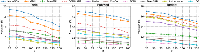
Figure 3. Performance comparison results (10-shot) w.r.t. Precision@K on three datasets. Figure best viewed in color.

Evaluation Metrics. In this paper, we use the following metrics to have a comprehensive evaluation of the performance of different anomaly detection methods:

• AUC-ROC is widely used in previous anomaly detection research (Ding et al., 2019b; Li et al., 2017). Area under curve (AUC) is interpreted as the probability that a randomly chosen anomaly receives a higher score than a randomly chosen normal object.

• AUC-PR is the area under the curve of precision against recall at different thresholds, and it only evaluates the performance on the positive class (i.e., abnormal objects). AUC-PR is computed as the average precision as defined in (Manning et al., 2008) and is used as the evaluation metric in  (Pang et al., 2019).

• Precision$\mathbf{@K}$ is defined as the proportion of true anomalies in a ranked list of $K$ objects. We obtain the ranking list in descending order according to the anomaly scores that are computed from a specific anomaly detection algorithm.

Implementation Details. Regarding the proposed GDN model, we use Simple Graph Convolution (Wu et al., 2019b) to build the network encoder with degree $K=2$ (two layers). As shown in Eq. (3), the abnormality valuator employs a two-layer neural network with one hidden layer of $512$ units followed by an output layer of $1$ unit. The confidence margin (i.e., $m$) in Eq. (7) is set as $5$ and the reference score (i.e., $\mu_{r}$) is computed using Eq. (5) from $k=5,000$ scores that are sampled from a Gaussian prior distribution, i.e., $\mathcal{N}(0,1)$. Unless otherwise specified, we set the total number of networks as $5$ ($4$ auxiliary networks and $1$ target network), and for each one we have access to $10$ labeled abnormal nodes that are randomly selected from the set of labeled anomalies ($\mathcal{V}^{L}$) in every run of the experiment.

For model training, the proposed GDN and Meta-GDN are trained with $1000$ epochs, with batch size $16$ in each epoch, and a $5$-step gradient update is leveraged to compute $\bm{\theta}^{\prime}$ in the meta-optimization process. The network-level learning rate $\alpha$ is $0.01$ and the meta-level learning rate $\beta=0.001$. Fine-tuning is performed on the target network where the corresponding nodes are split into $40\%$ for fine-tuning, $20\%$ for validation, and $40\%$ for testing. For all the comparison methods, we select the hyper-parameters with the best performance on the validation set and report the results on the test data of the target network for a fair comparison. Particularly, for all the network-based methods, the whole network structure and node attributes are accessible during training.

Table 3. Few-shot performance evaluation of Meta-GDN w.r.t. AUC-ROC and AUC-PR.

	Yelp		PubMed		Reddit
Setting	AUC-ROC	AUC-PR	AUC-ROC	AUC-PR	AUC-ROC	AUC-PR
$1$-shot	$0.702\pm 0.008$	$0.159\pm 0.015$	$0.742\pm 0.012$	$0.462\pm 0.013$	$0.821\pm 0.013$	$0.380\pm 0.011$
$3$-shot	$0.709\pm 0.006$	$0.164\pm 0.010$	$0.748\pm 0.008$	$0.468\pm 0.008$	$0.828\pm 0.012$	$0.386\pm 0.007$
$5$-shot	$0.717\pm 0.013$	$0.169\pm 0.007$	$0.753\pm 0.011$	$0.474\pm 0.005$	$0.834\pm 0.009$	$0.389\pm 0.008$
$10$-shot	$0.724\pm 0.012$	$0.175\pm 0.011$	$0.761\pm 0.014$	$0.485\pm 0.010$	$0.842\pm 0.011$	$0.395\pm 0.009$

5.2. Effectiveness Results (RQ1)

Overall Comparison. In the experiments, we evaluate the performance of the proposed framework Meta-GDN along with its base model GDN by comparing with the included baseline methods. We first present the evaluation results (10-shot) w.r.t. AUC-ROC and AUC-PR in Table 2 and the results w.r.t. Precision@K are visualized in Figure 3. Accordingly, we have the following observations, including: (1) in terms of AUC-ROC and AUC-PR, our approach Meta-GDN outperforms all the other compared methods by a significant margin. Meanwhile, the results w.r.t. Precision@K again demonstrate that Meta-GDN can better rank abnormal nodes on higher positions than other methods by estimating accurate anomaly scores; (2) unsupervised methods (e.g., DOMINANT, Radar) are not able to leverage supervised knowledge of labeled anomalies and therefore have limited performance. Semi-supervised methods (e.g., DeepSAD, SemiGNN) also fail to deliver satisfactory results. The possible explanation is that DeepSAD cannot model network information and SemiGNN requires a relatively large number of labeled data and multi-view data, which make them less effective in our evaluation; and (3) compared to the base model GDN, Meta-GDN is capable of extracting comprehensive meta-knowledge across multiple auxiliary networks by virtue of the cross-network meta-learning algorithm, which further enhances the detection performance on the target network.

Few-shot Evaluation. In order to verify the effectiveness of Meta-GDN in few-shot as well as one-shot network anomaly detection, we evaluate the performance of Meta-GDN with different numbers of labeled anomalies on the target network (i.e., $1$-shot, $3$-shot, $5$-shot and $10$-shot). Note that we respectively set the batch size $b$ to $2$, $4$, $8$, and $16$ to ensure that there is no duplication of labeled anomalies exist in a sampled training batch. Also, we keep the number of labeled anomalies on auxiliary networks as $10$. Table 3 summarizes the AUC-ROC/AUC-PR performance of Meta-GDN under different few-shot settings. By comparing the results in Table 2 and Table 3, we can see that even with only one labeled anomaly on the target network (i.e., $1$-shot), Meta-GDN can still achieve good performance and significantly outperforms all the baseline methods. In the meantime, we can clearly observe that the performance of Meta-GDN increases with the growth of the number of labeled anomalies, which demonstrates that Meta-GDN can be better fine-tuned on the target network with more labeled examples.

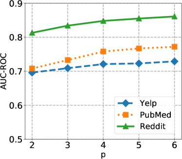
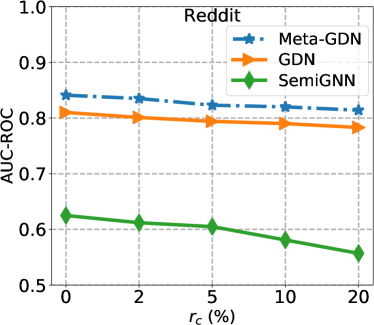
Figure 4. (a) Sensitivity analysis of Meta-GDN w.r.t. different number of auxiliary networks; (b) Model robustness study w.r.t. AUC-ROC with different contamination levels.

5.3. Sensitivity & Robustness Analysis (RQ2)

In this section, we further analyze the sensitivity and robustness of the proposed framework Meta-GDN. By providing different numbers of auxiliary networks during training, the model sensitivity results w.r.t. AUC-ROC are presented in Figure 4. Specifically, we can clearly find that (1) as the number of auxiliary networks increases, Meta-GDN achieves constantly stronger performance on all the three datasets. It shows that more auxiliary networks can provide better meta-knowledge during the training process, which is consistent with our intuition; (2) Meta-GDN can still achieve relatively good performance when training with a small number of auxiliary networks (e.g., $p=2$), which demonstrates the strong capability of its base model GDN. For example, on Yelp dataset, the performance barely drops $0.033$ if we change the number of auxiliary networks from $p=6$ to $p=2$.

As discussed in Sec. 4.1, we treat all the sampled nodes from unlabeled data as normal for computing the deviation loss. This simple strategy introduces anomaly contamination in the unlabeled training data. Due to the fact that $r_{c}$ is a small number in practice, our approach can work very well in a wide range of real-world datasets. To further investigate the robustness of Meta-GDN w.r.t. different contamination levels $r_{c}$ (i.e., the proportion of anomalies in the unlabeled training data), we report the evaluation results of Meta-GDN, GDN and the semi-supervised baseline method SemiGNN in Figure 4. As shown in the figure, though the performance of all the methods decreases with increasing contamination levels, both Meta-GDN and GDN are remarkably robust and can consistently outperform SemiGNN to a large extent.

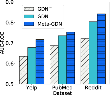
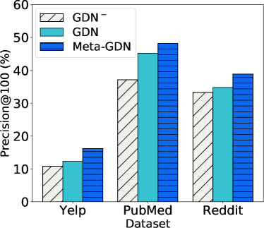
Figure 5. (a) AUC-ROC results of Meta-GDN and its variants; (b) Precision@100 results of Meta-GDN and its variants.

5.4. Ablation Study (RQ3)

Moreover, we conduct an ablation study to better examine the contribution of each key component in the proposed framework. In addition to Meta-GDN and its base model GDN, we include another variant GDN^- that excludes the network encoder and cross-network meta-learning in Meta-GDN. We present the results of AUC-ROC and Precision@100 in Figure 5 and Figure 5, respectively. The corresponding observations are two-fold: (1) by incorporating GNN-based network encoder, GDN largely outperforms GDN^- in anomaly detection on the target network. For example, GDN achieves $8.1\%$ performance improvement over GDN^- on PubMed in terms of precision@100. The main reason is that the GNN-based network encoder is able to extract topological information of nodes and to learn highly expressive node representations; and (2) the complete framework Meta-GDN performs consistently better than the base model GDN on all the three datasets. For instance, Meta-GDN improves AUC-ROC by $5.75\%$ over GDN on Yelp dataset, which verifies the effectiveness of the proposed cross-network meta-learning algorithm for extracting and transferring meta-knowledge across multiple auxiliary networks.

6. Conclusion

In this paper, we make the first investigation on the problem of few-shot cross-network anomaly detection. To tackle this problem, we first design a novel GNN architecture, GDN, which is capable of leveraging limited labeled anomalies to enforce statistically significant deviations between abnormal and normal nodes on an individual network. To further utilize the knowledge from auxiliary networks and enable few-shot anomaly detection on the target network, we propose a cross-network meta-learning approach, Meta-GDN, which is able to extract comprehensive meta-knowledge from multiple auxiliary networks in the same domain of the target network. Through extensive experimental evaluations, we demonstrate the superiority of Meta-GDN over the state-of-the-art methods.

References

- (1)
- Akoglu et al. (2015) Leman Akoglu, Hanghang Tong, and Danai Koutra. 2015. Graph based anomaly detection and description: a survey. DMKD (2015).
- Bandyopadhyay et al. (2019) Sambaran Bandyopadhyay, N Lokesh, and M Narasimha Murty. 2019. Outlier aware network embedding for attributed networks. In AAAI.
- Breunig et al. (2000) Markus M Breunig, Hans-Peter Kriegel, Raymond T Ng, and Jörg Sander. 2000. LOF: identifying density-based local outliers. In SIGMOD.
- Cao et al. (2016) Shaosheng Cao, Wei Lu, and Qiongkai Xu. 2016. Deep neural networks for learning graph representations. In AAAI.
- Ding et al. (2020a) Kaize Ding, Jundong Li, Nitin Agarwal, and Huan Liu. 2020a. Inductive anomaly detection on attributed networks. In IJCAI.
- Ding et al. (2019b) Kaize Ding, Jundong Li, Rohit Bhanushali, and Huan Liu. 2019b. Deep anomaly detection on attributed networks. In SDM.
- Ding et al. (2019a) Kaize Ding, Jundong Li, and Huan Liu. 2019a. Interactive anomaly detection on attributed networks. In WSDM.
- Ding et al. (2020b) Kaize Ding, Jianling Wang, Jundong Li, Kai Shu, Chenghao Liu, and Huan Liu. 2020b. Graph prototypical networks for few-shot learning on attributed networks. In CIKM.
- Dou et al. (2020) Yingtong Dou, Zhiwei Liu, Li Sun, Yutong Deng, Hao Peng, and Philip S Yu. 2020. Enhancing graph neural network-based fraud detectors against camouflaged fraudsters. In CIKM.
- Finn et al. (2017) Chelsea Finn, Pieter Abbeel, and Sergey Levine. 2017. Model-agnostic meta-learning for fast adaptation of deep networks. ICML (2017).
- Hadsell et al. (2006) Raia Hadsell, Sumit Chopra, and Yann LeCun. 2006. Dimensionality reduction by learning an invariant mapping. In CVPR.
- Hamilton et al. (2017) Will Hamilton, Zhitao Ying, and Jure Leskovec. 2017. Inductive representation learning on large graphs. In NeurIPS.
- Hochreiter et al. (2001) Sepp Hochreiter, A Steven Younger, and Peter R Conwell. 2001. Learning to learn using gradient descent. In ICANN.
- Kipf and Welling (2017) Thomas N. Kipf and Max Welling. 2017. Semi-Supervised Classification with Graph Convolutional Networks. In ICLR.
- Kriegel et al. (2011) Hans-Peter Kriegel, Peer Kroger, Erich Schubert, and Arthur Zimek. 2011. Interpreting and unifying outlier scores. In SDM.
- Li et al. (2019b) Ao Li, Zhou Qin, Runshi Liu, Yiqun Yang, and Dong Li. 2019b. Spam review detection with graph convolutional networks. In CIKM.
- Li et al. (2017) Jundong Li, Harsh Dani, Xia Hu, and Huan Liu. 2017. Radar: Residual Analysis for Anomaly Detection in Attributed Networks.. In IJCAI.
- Li et al. (2019a) Yuening Li, Xiao Huang, Jundong Li, Mengnan Du, and Na Zou. 2019a. SpecAE: Spectral AutoEncoder for Anomaly Detection in Attributed Networks. In CIKM.
- Liu et al. (2021) Lu Liu, Tianyi Zhou, Guodong Long, Jing Jiang, Xuanyi Dong, and Chengqi Zhang. 2021. Isometric Propagation Network for Generalized Zero-shot Learning. In ICLR.
- Liu et al. (2019) Lu Liu, Tianyi Zhou, Guodong Long, Jing Jiang, Lina Yao, and Chengqi Zhang. 2019. Prototype propagation networks (PPN) for weakly-supervised few-shot learning on category graph. In NeurIPS.
- Manning et al. (2008) Christopher D Manning, Hinrich Schütze, and Prabhakar Raghavan. 2008. Introduction to information retrieval. Cambridge university press.
- Müller et al. (2013) Emmanuel Müller, Patricia Iglesias Sánchez, Yvonne Mülle, and Klemens Böhm. 2013. Ranking outlier nodes in subspaces of attributed graphs. In ICDE Workshop.
- Pang et al. (2019) Guansong Pang, Chunhua Shen, and Anton van den Hengel. 2019. Deep anomaly detection with deviation networks. In KDD.
- Rayana and Akoglu (2015) Shebuti Rayana and Leman Akoglu. 2015. Collective opinion spam detection: Bridging review networks and metadata. In KDD.
- Ruff et al. (2020) Lukas Ruff, Robert A Vandermeulen, Nico Görnitz, Alexander Binder, Emmanuel Müller, Klaus-Robert Müller, and Marius Kloft. 2020. Deep Semi-Supervised Anomaly Detection. In ICLR.
- Sánchez et al. (2014) Patricia Iglesias Sánchez, Emmanuel Müller, Oretta Irmler, and Klemens Böhm. 2014. Local context selection for outlier ranking in graphs with multiple numeric node attributes. In SSDBM.
- Santoro et al. (2016) Adam Santoro, Sergey Bartunov, Matthew Botvinick, Daan Wierstra, and Timothy Lillicrap. 2016. Meta-learning with memory-augmented neural networks. In ICML.
- Sen et al. (2008) Prithviraj Sen, Galileo Namata, Mustafa Bilgic, Lise Getoor, Brian Galligher, and Tina Eliassi-Rad. 2008. Collective classification in network data. AI magazine (2008).
- Shen et al. (2020) Xiao Shen, Quanyu Dai, Fu-lai Chung, Wei Lu, and Kup-Sze Choi. 2020. Adversarial Deep Network Embedding for Cross-Network Node Classification.. In AAAI.
- Skillicorn (2007) David B Skillicorn. 2007. Detecting anomalies in graphs. In ISI.
- Song et al. (2007) Xiuyao Song, Mingxi Wu, Christopher Jermaine, and Sanjay Ranka. 2007. Conditional anomaly detection. TKDE (2007).
- Tang et al. (2008) Jie Tang, Jing Zhang, Limin Yao, Juanzi Li, Li Zhang, and Zhong Su. 2008. Arnetminer: extraction and mining of academic social networks. In KDD.
- Tang et al. (2020) Xianfeng Tang, Yandong Li, Yiwei Sun, Huaxiu Yao, Prasenjit Mitra, and Suhang Wang. 2020. Transferring Robustness for Graph Neural Network Against Poisoning Attacks. In WSDM.
- Tong and Lin (2011) Hanghang Tong and Ching-Yung Lin. 2011. Non-negative residual matrix factorization with application to graph anomaly detection. In SDM.
- Veličković et al. (2018) Petar Veličković, Guillem Cucurull, Arantxa Casanova, Adriana Romero, Pietro Lio, and Yoshua Bengio. 2018. Graph attention networks. In ICLR.
- Vinyals et al. (2016) Oriol Vinyals, Charles Blundell, Timothy Lillicrap, Daan Wierstra, et al. 2016. Matching networks for one shot learning. In NeurIPS.
- Wang et al. (2019) Daixin Wang, Jianbin Lin, Peng Cui, Quanhui Jia, Zhen Wang, Yanming Fang, Quan Yu, Jun Zhou, Shuang Yang, and Yuan Qi. 2019. A Semi-supervised Graph Attentive Network for Financial Fraud Detection. In ICDM.
- Wang et al. (2020) Ning Wang, Minnan Luo, Kaize Ding, Lingling Zhang, Jundong Li, and Qinghua Zheng. 2020. Graph Few-shot Learning with Attribute Matching. In CIKM.
- Wu et al. (2019b) Felix Wu, Tianyi Zhang, Amauri Holanda de Souza Jr, Christopher Fifty, Tao Yu, and Kilian Q Weinberger. 2019b. Simplifying graph convolutional networks. In ICML.
- Wu et al. (2019a) Man Wu, Shirui Pan, Lan Du, Ivor Tsang, Xingquan Zhu, and Bo Du. 2019a. Long-short Distance Aggregation Networks for Positive Unlabeled Graph Learning. In CIKM.
- Wu et al. (2020) Man Wu, Shirui Pan, Chuan Zhou, Xiaojun Chang, and Xingquan Zhu. 2020. Unsupervised Domain Adaptive Graph Convolutional Networks. In The Web Conference.
- Xu et al. (2019) Keyulu Xu, Weihua Hu, Jure Leskovec, and Stefanie Jegelka. 2019. How powerful are graph neural networks?. In ICLR.
- Xu et al. (2007) Xiaowei Xu, Nurcan Yuruk, Zhidan Feng, and Thomas AJ Schweiger. 2007. Scan: a structural clustering algorithm for networks. In Proceedings of the 13th ACM SIGKDD International Conference on Knowledge Discovery and Data mining (KDD).
- You et al. (2018) Jiaxuan You, Bowen Liu, Zhitao Ying, Vijay Pande, and Jure Leskovec. 2018. Graph convolutional policy network for goal-directed molecular graph generation. In NeurIPS.
- Zafarani et al. (2014) Reza Zafarani, Mohammad Ali Abbasi, and Huan Liu. 2014. Social media mining: an introduction. Cambridge University Press.
- Zhang et al. (2010) Yin Zhang, Rong Jin, and Zhi-Hua Zhou. 2010. Understanding bag-of-words model: a statistical framework. IJMLC (2010).
- Zhang et al. (2019) Zhen-Yu Zhang, Peng Zhao, Yuan Jiang, and Zhi-Hua Zhou. 2019. Learning from incomplete and inaccurate supervision. In KDD.
- Zhao et al. (2020) Tong Zhao, Chuchen Deng, Kaifeng Yu, Tianwen Jiang, Daheng Wang, and Meng Jiang. 2020. Error-Bounded Graph Anomaly Loss for GNNs. In CIKM.
- Zhou and Paffenroth (2017) Chong Zhou and Randy C Paffenroth. 2017. Anomaly detection with robust deep autoencoders. In KDD.
- Zhou et al. (2018) Dawei Zhou, Jingrui He, Hongxia Yang, and Wei Fan. 2018. Sparc: Self-paced network representation for few-shot rare category characterization. In KDD.
- Zhou et al. (2020) Fan Zhou, Chengtai Cao, Goce Trajcevski, Kunpeng Zhang, Ting Zhong, and Ji Geng. 2020. Fast Network Alignment via Graph Meta-Learning. In INFOCOM.
- Zhou et al. (2019b) Qinghai Zhou, Liangyue Li, Nan Cao, Lei Ying, and Hanghang Tong. 2019b. ADMIRING: Adversarial multi-network mining. In ICDM.
- Zhou et al. (2019a) Qinghai Zhou, Liangyue Li, and Hanghang Tong. 2019a. Towards Real Time Team Optimization. In Big Data.
- Zügner and Günnemann (2019) Daniel Zügner and Stephan Günnemann. 2019. Adversarial Attacks on Graph Neural Networks via Meta Learning. In ICLR.