Simple pair-potentials and pseudo-potentials for warm-dense matter applications.

Abstract

We present computationally simple parameter-free pair potentials useful for solids, liquids and plasma at arbitrary temperatures. They successfully treat warm-dense matter (WDM) systems like carbon or silicon with complex tetrahedral or other structural bonding features. Density functional theory asserts that only one-body electron densities, and one-body ion densities are needed for a complete description of electron-ion systems. DFT is used here to reduce both the electron many-body problem and the ion many-body problem to an exact one-body problem, namely that of the neutral pseudoatom (NPA). We compare the Stillinger-Weber (SW) class of multi-center potentials, the embedded-atom approaches and $N$-atom DFT, with the one-atom DFT approach of the NPA to show that many-ion effects are systematically included in this one-center method via one-body exchange-correlation functionals. This computationally highly efficient one-center DFT-NPA approach is contrasted with the usual $N$-center DFT calculations that are coupled with molecular dynamics (MD) simulations to equilibriate the ion distribution. Comparisons are given with the pair-potential parts of the SW, ‘glue’ models, and the corresponding NPA pair-potentials to elucidate how the NPA potentials capture many-center effects using single-center one-body densities.

I Introduction

Condensed-matter systems at temperatures $T\geq 0$, where the constituents may be neutral or ionized, solid or fluid, are included in the appellation “ warm dense matter” (WDM). The reference to “dense” pertains mostly to the property of strong interactions rather than to ‘density’ per se. Furthermore, ‘warm’ systems are those away from the simplifications available for the $T\to 0$ or $T\to\infty$ limits. Hence a truly general finite-$T$ many-body theory of interacting electrons and ions in arbitrary states of matter is needed as our focus is on first-principles methods. Density functional theory (DFT) is a favoured approach since it reduces such problems to a theory of mere one-body densities, requiring no multi-atom approaches, at least in principle. Here we exploit DFT for simplifying the general electron-ion problem to the fullest ilciacco93 ; cdw-N-rep19 .

While typical WDM systems are in the domain of plasma physics, laser-matter interactions, high pressure physics, geophysics, astrophysics etc., many problems in nano-structure physics also fall into WDM physics. An electron layer or a hole layer in a quantum well contains particles of modified effective mass ($m^{*}$) that may be a tenth of the free electron mass. The corresponding Fermi energies and particle densities are such that even at room temperature, the electrons may be partially degenerate while the holes are classical particles, the system behaving as warm-dense matter lfc1-dw19 . The quantum wells or nanostructures may have metal-oxide layers and inhomogenieties that need a unified many-body first principles theory 2v2d04 .

The need for practical computations of energetics of defects and dislocations in metallic structures led to semi-empirical theories usually known as embedded-atom or effective medium theories DawFoilsBasks93 . The potential $V(\vec{R})$ felt by an ion at $\vec{R}$ is modeled using two-body, three-body and possibly higher terms in the energy, and used to motivate functional forms for numerically fitted representations of structure dependent energies.

A parallel development in semiconductor physics modified the usual two-body potentials of ‘covalent bonds’ (e.g., of the Lenard-Jones type) with ‘structure dependent’ three-body terms, viz., as in the well-known Stillinger-Weber SW85 or Tersoff models Ters88 for C, Si and other tetrahedral solids and fluids. These have been extended to include empirical ‘bond-order’, angular and ‘torsional’ correlations ghiring05 , producing very complex ‘potentials’. Highly parameter-loaded potentials fitted to empirical data as well as large DFT data bases OQMD have emerged. Many of these multi-center multi-parameter potentials have been incorporated in codes like LAMMPS (Large-scale Atomic/Molecular Massively Parallel Simulator) LAMMPS95 for regular use in molecular dynamics (MD) simulations. In this approach, the electron system is fully integrated out and only a classical simulation based on the multi center potentials is used. Hence these multi-center effective-medium models lack associated atomic pseudopotentials that may be used to delineate their building blocks, or for use in transport studies. In contrast, the NPA potentials that we discuss here relate directly to underlying pseudopotentials, response functions, and XC-functionals as the NPA is based on first-principles physics. It also includes the multi-center ‘effective medium’ effects via ion-ion XC-functionals generated in situ.

Attempts to extend these multi-center potentials, and use $N$-center DFT for $T>0$ applications to complex systems like, say, WDM plastics hamelCH12 , have exploited increasing computer power without change in the conceptual framework. However, such attempts have yielded disappointing results, esp. with respect to WDM applications. Thus, SW and similar potentials predict spurious phase transitions for liquid carbon glosli99 ; WuLPT02 , while the Tersoff potential over-estimates the melting point of silicon by $\sim$ 50%. Similarly, Kraus et al kraus13 found that sophisticated ‘bond-order’ potentials available for carbon failed badly for their study of liquid-carbon at 100 GPa.

In the following we argue, and provide realistic examples to show that these empirical data-fitting approaches, be they at the level of Stillinger-Weber (SW) SW85 , or bond-order potentials, or with “high through-put data-base fittings” OQMD , are in fact not necessary, at least for fluids and systems with some simplifying symmetries, if the full power of DFT is exploited. However, $N$-atom DFT is necessary and best used to provide first-principles benchmarks for other methods including one-atom DFT methods.

If we consider an electron-ion system in equilibrium at the temperature $T$, with a one-body electron density $n(\vec{r})$, and a one-body ion density $\rho(\vec{r})$, standard DFT asserts that all the thermodynamic properties and linear transport properties are a functional of just the one-body $n(r)$ and $\rho(r)$, while the many-body interactions are also functionals of just these one body densities. Hence multi-center approaches should not be necessary if DFT is rigorously applied. The many-body effects are relegated to the exchange-correlation (XC) functionals. The functionals are non-local but remain one-body density functionals. At finite-$T$ we use the free-energy functionals $F_{ss^{\prime}}^{xc}[n_{s},n_{s^{\prime}}]$, where $s$ or $s^{\prime}=e,i$ is the species index, with $n_{e}=n(r),n_{i}=\rho(r)$ ilciacco93 . The finite-$T$ free-energy functionals reduce to the usual ground-state energy functionals at $T=0$.

Common computer implementations of DFT in large codes like ABINIT ABINIT or VASP VASP explicitly require the locations $\vec{R}_{I},I=1,N$, of the nuclei of $N$ ions and only the electron problem is reduced by DFT. The density functional theory of the one-body ion density $\rho(r)$ is not invoked in these codes, although the DFT for classical ions begun to be exploited since the 1970s, e.g., Evans EvansDFT79 . Only an electron exchange-correlation functional $F_{ee}^{xc}$ is invoked in VASP or ABINIT, using a Kohn-Sham (KS) calculation for specific ionic configuration ${\vec{R}_{I}}$ using the Born-Oppenheimer (BO) approximation. The ions merely provide an ‘external potential’. Classical molecular dynamics is used to equilibrate the ion distribution $\sum\delta(\vec{r}-\vec{R_{I}})$. Such an approach produces a many-centered potential energy function $V({\vec{R}_{1},\cdots,\vec{R}_{N}})$. So, single-ion properties, pair-potentials between ions etc., are not directly available by this $N$-center DFT, as the calculation is for a solid with a unit cell of $N$-nuclei and electrons moving on a complex potential-energy surface.

Extraction of ‘atomic’ properties invokes an expansion of, say, the potential felt by an ion at $\vec{R}$ in terms two-body, three-body and higher interactions. A truncation in finite order and fitting a required property, e.g., an effective potential, to a large parameter set is used. If individual atomic properties, e.g., charge state $\bar{Z}$, X-ray Thomson Scattering (XRTS) profiles etc., are needed, the $N$-atom cluster has to be decomposed using some additional model Plage-XRTS15 ; BethkenZbar20 for ‘decomposing’ the cluster into contributions from individual atomic centers. In effect, these methods attempt to reconstruct the Neutral-Pseudo-Atom result from the $N$-atom DFT calculation. Usually $N$ ranges from 100-500 particles unless crystal symmetry or some such property can be invoked.

A kinetic energy functional Karas18 may be used to simplify the DFT computations if some accuracy could be sacrificed, but ‘one-atom’ properties or pair-potentials are not directly available from such $N$-ion calculations either.

The explicit dynamical evolution of atomic positions used in large codes ABINIT ; VASP works well for solid-state physics applications based on the unit cell, or for the quantum chemistry of a finite number of atoms usually at $T=0$. They provide microscopic details of ‘bonding’ between atoms not available from the NPA. The NPA gives only a thermodynamic average of the system, via the thermodynamic one-body densities $n(r),\rho(r)$. In constructing the NPA that reduces the $N$ center problem to a single center, we explicitly identify only one nucleus and then consider the one-body distributions $n_{s}(r),s=e,i$ around it rather than their explicit positions, and exploit the spherical symmetry of liquids and plasmas, or the crystal symmetry of solids, to provide a computationally very efficient and yet completely rigorous scheme. The generalization to mixtures containing many species increases the number of XC-functionals needed, and may proceed as in Ref. eos95 . The NPA theory of mixtures will be illustrated by some explicit examples.

Use of DFT for the ion distribution avoids the ad hoc introduction of multi-atom effects found in semi-empirical potentials like the Stillinger-Weber potentials, effective medium models, or in the Finnis-Sinclair potentials Finnis-Sinc09 used in metal physics. We have shown that a systematic procedure based on the Ornstein-Zernike equation exists for including the three-body and higher terms into the ionic XC-functional $F_{ii}^{xc}$. Since ions are classical particles in most cases, the ‘exchange’ content of $F_{ii}^{xc}$ is negligible.

Unlike fitted potentials, the NPA method, being a first principles approach, can be used for unusual states of matter. If the electron subsystem is at a temperature $T_{e}$, and the ions subsystem is at a temperature $T_{i}$, we have one body densities $n_{e}(r,T_{e})$ and $\rho(r,T_{i})$ defining a two-temperature WDM system. A quasi-equilibrium exists due to the slowness of the energy relaxation via electron-ion collisions. Then a quasi-thermodynamic situation exists for time scales $\tau$ such that $\tau_{ee}\ll\tau\ll\tau_{ii}\ll\tau_{ei}$, where $\tau_{ss^{\prime}}$ is the temperature relaxation time cargese94 between species $s$ and $s^{\prime}$. Then the NPA approach can be generalized to two-temperature WDMs and explicit NPA calculations are available HarbourDSF18 ; cargese94 .

Although the potentials in NPA are constructed in linear response theory, they include the non-linear effects brought in via the Kohn-Sham atomic calculation. Hence the method is applicable to a wide range of densities and temperatures. Here we examine simple fluids, mixtures of fluids, and complex fluids like Si, containing transient covalent bonds, from low $T$ to high $T$. Examples where linear-response fails are, for instance, liquid-C and liquid transition metals at low $\rho,T$ Stanek21 , where special procedures are needed, even in standard DFT.

However, in general, it is found that these NPA pair-potentials work better than common multi-center potentials, and inexpensively recover pair-distribution functions and other properties in good agreement with the best available DFT simulations, for well studies systems like Al, Be, Li, etc., and for complex fluids like C, Si and Ge. NPA calculations recover the properties of supercooled liquid Si at 2.57 g/cm³ just below the melting point of silicon, with only a fraction of the computation effort needed using VASP-type $N$-center calculations cdwSi20 .

The NPA, based on the two-component DFT of ions and electrons enable complex WDM calculations to be reduced to simple one center Kohn-Sham calculations that require nothing more than a laptop since the NPA is computationally very like an average-atom calculation. But these reach the accuracy of standard DFT calculations implemented by large codes like ABINIT ABINIT or VASP VASP , where advanced gradient-corrected meta functionals have to be used because the $N$-center electron density is very complex and highly non-uniform.

The NPA approach can impact WDM research as follows. (i) The method is applicable to metallic solids, liquids or plasmas from very low $T$ to very high $T$. (ii) It usually provides reliable one-atom properties like pseudopotentials, charge states $Z^{j+}$, atomic eigenfunctions, phase shifts, densities of states etc. (iii) It provides pair properties like pair-potentials, structure factors and pair-distribution functions (PDFs) needed in calculating optical and transport properties of matter. (iv) It provides a rigorous, rapid many-body calculation of the ionization balance and thermodynamics, including composition fractions $x_{j}$ of mixtures of ionization states $Z^{j+}$. (v) It has proven useful in studying two-temperature non-equilibrium systems and temperature relaxation rates. (vi) Its rapidity and wide $\rho,T$ applicability enables easier uncovering of phase transitions etc., as shown recently for liquid silicon at its melting point cdwSi20 and in WDM states, or for liquid carbon CPP-carb18 ; DWP-carb90 . (vii) It provides a transparent physical model based on DFT, without ad hoc fit parameters. (viii) Its rapidity and simplicity enables easy incorporation in large dynamical calculations. The limitations of the method are similar to those of DFT. Additionally, the one-atom DFT implemented in the NPA is not successful for systems with low free-electron densities at low $T$.

In the following we present our theory of pair potentials as follows. The NPA is introduced as a rigorous DFT concept and then various simplifications are indicated. We present a computational procedure for determining the equilibrium one-body densities $n(r),\rho(r)$, and the needed XC-functionals. Then we derive simple linear-response pseudo-potentials from the $n(r)$ so obtained. These pseudopotentials apply to interactions mediated by the continuum electrons, also called valance electrons, metallic electrons, or ‘free electrons’. The atomic cores are described by the bound states obtained from the NPA calculation. The pseudopotentials and bound-densities are used to construct bound-bound, bound-free, and free-free contributions to the pair potentials. Van der Waals type interactions occur in the bound-bound interactions. Then we compare our potentials with SW type multi-center potentials, and also with effective medium theories. It is noted that, unlike the short-ranged potentials of multi-center empirical models, the long-range pair-potentials of the NPA, with many minima that register with the second, third and higher neighbour effects in the pair-distribution functions, bring in multi-ion correlations. An analysis of the potential felt by an ion in a fluid is used to show how these effects are included via the Ornstein-Zernike equation and the modified hyper-netted chain equation. Examples are given, including a comparison with the 40 parameter ‘glue potential’ for aluminum from effective-medium theory.

II Details of the NPA model

A brief description of the NPA model is given for convenience and for defining the notation used. Hartree atomic units ($|e|=\bar{h}=m_{e}=1$) will be used unless otherwise specified. The systems explicitly studied are warm-dense fluids and hence have spherical symmetry, although the NPA method applies equally well to low-temperature crystalline solids Ziman67 ; Dagens72 ; Pe-Be . An application to surface ablation and hot phonons has been reported, e.g., HarbEOSPhn17 recently. However, the early NPA model (e.g., of Ziman) sought mainly to create a computationally convenient short-ranged object named the NPA, so that inconvenient long-ranged Coulomb fields of the ionic charges are neutralized.

The objective of the NPA model used here cdw-N-rep19 ; eos95 ; Pe-Be is to implement a simplification of the full DFT model for electrons and ions given in Ref DWP1 and illustrated by an application to hydrogen. Its objectives have to be distinguished from early NPA models, or from various currently-available ion-sphere (IS) or average-atom (AA) models SternZbar07 ; Rosznayi08 ; FausAA10 ; PironBlenski11 ; Murillo13 ; StarretHam14 ; YongHou-AA-17 implemented in various laboratories. Many of them invoke simplifications which are outside DFT. In fact, the early formulations used an expansion of the ion-ion interactions in one-body, two-body, etc., contributions and invoked assumptions of non-overlapping electron distributions, superposition approximations, neglect of higher order ionic and electronic correlations. They also invoked the Born-Oppenheimer approximation. The formal theory of the NPA does not need any of these assumptions and includes higher-order effects via XC-functionals DWP1 . However, some of these approximations are invoked Pe-Be ; eos95 for numerical simplicity.

Our NPA model DWP1 ; Pe-Be ; eos95 is based on the variational property of the grand potential $\Omega([n],[\rho])$ as a functional of the one-body densities $n(r)$ for electrons, and $\rho(r)$ for ions, even though some indicated references, e.g., Ref. Pe-Be use a more conventional liquid-metal type of presentation. The Hohenberg-Kohn theorem applies equally to electrons or ions EvansDFT79 ; DWP1 . Only a single nucleus of the material to be studied is used and taken as the center of the coordinate system. The other ions (“field ions”) are replaced by their one-body density distribution $\rho(r)$ as DFT asserts that the physics is solely given by the one-body distribution; i.e., we do not discard two-body, three-body, and such information as they get included via exchange-correlation (XC)-functionals. That is, there is no ‘mean-field’ approximation used. Furthermore, in the case of ions, the exchange effects are usually negligible although the ion-ion many-body functional will also be called an XC-functional for generality.

Hence unlike in $N$-center DFT codes like the VASP or ABINIT, the NPA is a type of one-center DFT using DFT in its full sense. Consequently, there is no highly inhomogeneous multi-ion potential energy surface, or a complex electron distribution resident on such a multi-center potential energy surface. Hence a local-density approximation (LDA) to the electron XC-functional can be sufficient and no gradient expansions are needed. In our calculations we have used the finite-$T$ electron XC-functional by Perrot and Dharma-wardana PDWXC in LDA, while most large-scale codes implement $T=0$ XC-functionals like the PBE functional PBE96 . These include generalized gradient corrections, and other advanced but computationally very demanding functionals, e.g., the SCAN functional SCAN13 . It is seen that our NPA-LDA calculations are in close agreement with $N$-atom DFT calculations using the PBE or SCAN functionals even for complex transiently bonded liquids like molten Si cdwSi20 or liquid carbon CPP-carb18 , with the VASP results disconcertingly dependent on the choice of the XC-functional Remsing17 . Our finite-$T$ functional used is in good agreement with quantum Monte-Carlo XC-data cdw-N-rep19 in the density and temperature regimes of interest.

The artifice of using a nucleus at the origin converts the one-body ion density $\rho(r)$ and the electron density $n(r)$ into effective two body densities in the sense that

$$\rho(r)=\bar{\rho}g_{ii}(r),\;n(r)=\bar{n}g_{ei}(r).$$ (1)

The ion at the origin need not be at rest. However, most ions are heavy enough that the Born-Oppenheimer approximation is valid. Here $\bar{\rho},\bar{n}$ are the average ion density and the average free electron density respectively, and prevail far away from the central nucleus. Any bound electrons are assumed to be firmly associated with each ionic nucleus and contained in their “ion cores” of radius $r_{c}$ such that

$$r_{c}<r_{\rm ws},\;r_{ws}=\left[3/4\pi\bar{\rho}\right]^{1/3}.$$ (2)

Here $r_{\rm ws}$ is the Wigner-Seitz radius of the ions. The corresponding electron sphere radius, based on $\bar{n}$ is denoted by $r_{s}$. In some cases, e.g., for some transition metals, and for continuum resonances etc., this condition for a compact core may not be met, and additional steps are needed. We assume that $r_{c}<r_{ws}$ unless stated otherwise. The DFT variational equations used here are:

$$\frac{\delta\Omega[n,\rho]}{\delta n} = 0$$ (3)

$$\frac{\delta\Omega[n,\rho]}{\delta\rho} = 0.$$ (4)

These directly lead to two coupled KS equations where the unknown quantities are the XC-functional for the electrons, the ion XC-functional, and the electron-ion XC functional ilciacco93 . If the Born-Oppenheimer approximation is imposed, the electron-ion XC-functional may also be neglected. Approximations arise in modeling these functionals and in simplifying the decoupling of the two KS equations eos95 ; CPP15 . The first equation gives the usual Kohn-Sham equation for electrons moving in the external potential of the ions. This is the only DFT equation used in the $N$-center DFT-MD method implemented in standard codes like the VASP, where the ions define a periodic solid whose structure is varied via $N$-atom classical MD, followed by a Kohn-Sham solution at each step.

In the NPA the one-body ion density $\rho(r)$ rather than an $N$-center ion density is used. It was shown in  DWP1 that the DFT equation for the one-body ion density can be identified as a Boltzmann-like distribution of field ions around the central ion, distributed according to the ‘potential of mean force’ well known in the theory of fluids. Hence the ion-ion correlation functional $F_{ii}^{xc}$ was identified to be exactly given by the sum of hyper-netted-chain (HNC) diagrams plus the bridge diagrams. The bridge diagrams have to be approximated from a hard-sphere fluid LFA83 , or evaluated using MD.

The mean electron density $\bar{n}$ can also be specified as the number of free electrons per ion, viz., the mean ionization state $Z$. It is also denoted as $\bar{Z}$ since a plasma containing a mixture of ionization states $Z^{j+}$ with composition fractions $x_{j}$ will appear as a single average ion of charge $\bar{Z}=\sum_{j}x_{j}Z^{j+}$. This average description can be sharpened by constructing individual NPA models for each integer ionization and using them in the thermodynamic average eos95 . Hence the NPA approach yields the composition fractions $x_{j}$ in the plasma, although the ABINIT and VASP calculations cannot yield such information directly. Unfortunately, the partitioning of the $N$-atom density from $N$-atom results into individual atomic contributions is not unique and a variety of schemes exist Li-Parr86 ; Francisco06 ; BethkenZbar20 .

Although the material density $\bar{\rho}$ is specified, the mean free electron density $\bar{n}$ is initially unknown at any given temperature, as it depends on the ionization balance which is controlled by the free energy minimization implied by the DFT Eq. 3. Hence a trial value for $\bar{n}$, i.e, equivalently, a trial value for $\bar{Z}$, is assumed in the NPA and the thermodynamically consistent $\rho(r)$ is determined. This is repeated till the target mean ion density $\bar{\rho}$ is obtained. This also implies that NPA implements a calculation of the ionization balance in the system. In effect, a full many-body extension of the Saha equation via its DFT free-energy minimum property is implemented in the NPA model.

The mean number of electrons per ion, viz., $\bar{Z}$, is often replaced by $Z$ in this paper when no confusion arises. It is an experimentally measurable quantity. It is routinely measured using Langmuir probes Smy76 in atmospheric and gas discharge plasmas, or from optical and other measurements of appropriate properties, e.g., the conductivity and the XRTS profile GlenzerRedmer2009 for general WDM systems. The argument that ‘there is no quantum mechanical operator’ corresponding to $\bar{Z}$, and hence it is not an observable, is incorrect. The system studied is not a pure quantum system but a system attached to a classical heat bath. Here $T,\mu,\bar{Z}$ are Lagrange multipliers associated with the conservation of energy, particle number, and charge conservation respectively. They do not correspond to simple quantum operators whose mean values are $T,\mu$ or $\bar{Z}$, although complicated operator constructions can be given.

II.1 Computational simplifications

The Kohn-Sham equation has to be solved for a single electron moving in the field of the central ion surrounded by $n(r),\rho(r)$. The ion distribution $\rho(r)=\bar{\rho}g(r)$ associated with it is also modified at each iteration with a corresponding modification of the trial $\bar{Z}$ until the target density $\rho$ is obtained. However, it was noticed very early Pe-Be ; eos95 that the Kohn-Sham solution was quite insensitive to the details of the $g(r)$ in most cases; an example of an exception being low-density liquid carbon at low $T$. Hence a simplification was possible DWP1 ; Pe-Be ; eos95 . The simplification was to replace the trial $g(r)$ at the trial $\bar{Z}$ by a cavity-like distribution:

$$g_{cav}(r) = 0,r\leq r_{\rm ws},\;g_{cav}(r)=1,\;r>r_{\rm ws}$$ (5)

$$\rho_{cav}(r) = \bar{\rho}g_{cav}(r),$$ (6)

$$V_{cav}(k) = V_{k}\bar{Z}(3/K)^{3}\left[\sin(K)-K\cos(K)\right]$$ (7)

$$V_{k} = 4\pi/k^{2},\;K=kr_{\rm ws}.$$ (8)

Here the $r_{\rm ws}$ is the trial value of the ion Wigner-Seitz radius, based on the trial $\bar{n}$. Convergence of the equations using the cavity approximation instead of the full $g(r)$ is very rapid, since adjusting the $g_{cav}(r)$ at each iteration requires only adjusting the trial $r_{\rm ws}$ to achieve self-consistency. The self-consistency in the ion distribution is rigorously controlled by the Friedel sum rule for the phase shifts of the KS-electrons DWP1 . This ensures that $\bar{\rho}=\bar{n}/Z$. Thus, a valuable result of the calculation is the self-consistent value of the mean ionization state $Z$, which is both an atomic quantity and a thermodynamic quantity. Here too we note that a sophisticated quantum many-body version of a Saha equation is also solved automatically within this DFT calculation in determining $\bar{Z}$. The pseudopotentials, pair-potentials, the equation of state (EOS) etc., depend directly on the accuracy of $\bar{Z}$. In contrast, many average-atom models use various prescriptions based on ion-sphere models (valid at high-$T$) to determine $\bar{Z}$ SternZbar07 ; Murillo13 .

In early discussions of the neutral pseudoatom as applied to solids Dagens72 ; Ziman67 , no attempt was made to introduce a DFT of the ions, and an analytically convenient potential neutralizing the long-range Coulomb interaction of the central ion was added to produce a computationally convenient object with a short-ranged potential. In such studies, and in MD simulations of Coulomb potentials, a neutralizing Gaussian charge distribution is sometimes used. The spherical cavity model used here is a good approximation to a typical ion-ion $g(r)$ for $r<r_{ws}$.

Here we note several simplification used in implementing the NPA. Given that the electron distribution $n(r)$ obtained self consistently can be written as a core-electron (i.e., bound electron) term and a free-electron term when the core electrons are compactly inside the ion Wigner-Seitz sphere, we have:

$$n(r) = n_{c}(r)+n_{f}(r),\;\Delta n_{f}(r)=n_{f}(r)-\bar{n}$$ (9)

$$a_{f}(r) = \Delta n_{f}(r).$$ (10)

The core-electron density (made up of “bound electrons”) is denoted by $n_{c}(r)$. The free electron density $n_{f}(r)$ is the response of an electron fluid (see sec. III.3) to the central ion and to an ion-density deficit (a cavity) near the central ion that mimics $\rho(r)$. It contributes to the potential acting on the electrons. The response of a uniform electron fluid (i.e., without the cavity) to the central ion can be obtained by subtracting out the effect of the cavity using the known static interacting linear response function $\chi(k,\bar{n},T)$ of the electron fluid. That is, from now on we take it that the charge density $n_{f}(r)$ and the density pile up $\Delta n_{f}(r)$ are both corrected for the presence of the cavity. However, we use the same symbols as before when no confusion arises. Furthermore, in dealing with atoms ‘a’, ‘b’ etc, we refer to the ‘density pileup’ or displaced free electron density $\Delta n_{f}(r)$ as $a_{f}(r)$, with its Fourier transform denoted by $a_{f}(k)$.

In Fig. 1(a) we display the calculated $n_{f}(r)$ for an Aluminum ion in a hot plasma. Unlike in ABINIT or the VASP where core electrons are subsumed in a pseudopotential, the NPA uses all-electron atomic calculations and provides the true core-electron density as well.

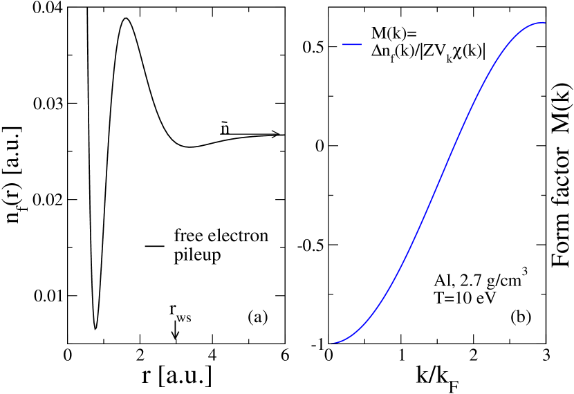
Figure 1: (Online color) Panel (a). The free electron density $n_{f}(r)$ around an Al nucleus in its electron fluid of average density $\bar{n}$ corresponding to $\bar{Z}=3$, $\rho=2.7$g/cm³, at 10 eV. The bound electron core is inside $r_{ws}$, and $n_{f}(r)$ develops oscillations as the free-electron states are orthogonal to core states. Panel (b). The $k$- dependent pseudopotential form factor $M(k)$, calculated from the electron pileup $\Delta n_{f}(k)$ and the electron response function $\chi(k,T)$. Here $V_{k}$ is the Coulomb potential $4\pi/k^{2}$. The large $k/k_{F}>2$ behaviour is unimportant unless $T>E_{F}$. Here $k_{F}$ is the Fermi wave vector.

A key difference between many average-atom models and the NPA is that the free electrons are not confined to the Wigner-Seitz sphere, but move in all of space represented by a very large ‘correlation sphere’ of radius $R_{c}$. This may be ten to twenty times the Wigner-Seitz radius of the central ion eos95 ; Murillo13 . This ensures that the small-$k$ limit of the structure factor $S(k)$ is accurately obtained.

III Pseudopotentials and Pair-potentials from the NPA model.

As the NPA reduces the multi-center WDM to a single ion and its environment described by $n(r),\rho(r)$, pair potentials must be constructed from the appropriate one body distributions, viz, the core-electron density $n_{c}(r)$, and the ‘free’ electron density $n_{f}(r)$.

The pseudopotential $U_{ei}(r)$, or its Fourier transformed form $U_{ei}(k)$ enables a rigorous and useful separation of the contributions of bound and free charge densities to the pair potential which is a two-center property. We constructed it from one-center results to avoid two-center computations. Thus the pseudopotential is constructed to be a linear response property where possible. In fact, unlike in crystals, the spherical symmetry of fluids allows one to use simple local pseudopotentials, without having to deal with angular-momentum dependent (i.e., nonlocal) pseudopotentials. So these potentials use only an $s$-wave component and differ from those used in the $N$-center DFT codes. They are also constructed to be weak potentials, allowing the use of second-order perturbation theory with them.

Unlike non-linear pseudopotentials used in ABINIT or VASP, these pseudopotentials are $\rho,T$ dependent, and constructed in situ during the calculation. The range of validity of such linearized pseudopotentials has been discussed elsewhere cdw-Utah12 .

A rigorous discussion of pair-potentials $U_{\rm ab}$ between two atoms of species ‘a’, and ‘b’, including the effect of core electrons is given in the Appendix B of Ref. eos95 . Core-core interactions are important for atoms including and beyond argon, viz., Na, K, Au, etc., with large cores and zero or low $\bar{Z}$. In contrast, core-core interactions in high $Z$ ions like Al³⁺, Si⁴⁺ at normal density are very small in comparison to the interactions via free electrons.

We illustrate the calculation of core-core interactions by a discussion of the weakly ionized argon WDM system. The core electron distributions $n_{c}(r)$ of the atom ‘a’ is denoted by $a_{c}$, while $a_{f}$ denotes the displaced free electron distribution, $\delta n_{f}(r)$, for the atomic center of type ‘a’ (and similarly for ‘b’). The total pair-interaction $V_{ab}$ is of the form:

$$V_{\rm ab} = V(a_{c},b_{c})+V(a_{c},b_{f})+V(a_{f},b_{c})+V(a_{f},b_{f})$$ (11)

$$= V^{cc}(r)+V^{cf}(r)+V^{ff}(r).$$

These terms will be discussed separately.

III.1 The interaction mediated by free electrons

The last term of Eq. 11, viz., $V^{ff}(r)$ is the familiar ion-ion interaction mediated by metallic electrons. This is adequately evaluated in second-order perturbation theory when the interactions are weakened by electron screening. The linearized electron-ion pseudopotential described below can be used for WDM systems and liquid metals unless the free electron density and the temperature ($T/E_{F}$) are low, when linear-response methods become invalid. In fact, when the pair-potential develops a negative region significantly larger than the thermal energy, permanent chemical bonds are formed; then the liner-response methods used here cannot be used.

The electron-ion pseudopotential $U_{\rm a}^{ei}(k)$ of the ion ‘a’ is evaluated in $k$-space via the displaced free-electron density $a_{f}(k)$, and the electron response function $\chi(k,T)$. The pseudopotential is:

$$U_{\rm a}^{ei}(k) = a_{f}(k)/\chi(k,T)$$ (12)

$$= -Z_{a}V_{k}M(k),\;V_{k}=4\pi/k^{2}.$$ (13)

Here $M(k)$ is the form factor of the pseudopotential (see Fig. 1). The NPA calculation via Eq. 12 automatically yields the pseudopotential inclusive of a form factor. This may be fitted to a Heine-Abarankov form which fits a core radius $r_{c}$ and a constant core potential $V_{c}$. Alternatively, a more complex parameterized form may be needed, as in Ref. cdw-Utah12 . However, using the numerical tabulation of $U_{\rm a}^{ei}(k)$ is more accurate and avoids the fitting step.

The fully interacting linear response function $\chi(k,T)$ of the uniform electron fluid at the temperature $T$ is discussed in sec. III.3. So, for identical ions ‘a’, we have the form:

$$V_{\rm aa}^{ff}(k) = Z_{a}^{2}V_{k}+|U_{\rm a}^{ei}(k)|^{2}\chi(k,T)$$ (14)

$$= Z_{a}^{2}V_{k}+|a_{f}(k)|^{2}/\chi(k,T).$$ (15)

In the case of two different atomic species, we readily have:

$$V_{\rm ab}^{ff}(k) = Z_{a}Z_{b}V_{k}+$$ (17)

$$|U_{\rm a}(k)U_{\rm b}(k)|\chi(k,T).$$

In the NPA theory for mixtures, $Z_{a}$ and $Z_{b}$ are integers, while in the simple average-atom form of the NPA, the mean value $\bar{Z_{s}}=\Sigma_{s}x_{s}Z_{s}$ is used to represent the mixture with composition fractions $x_{s}$ via a single calculation. In a mixture calculation, separate NPA calculations for each component are needed.

The simplest pseudopotential, valid for point ions, $r_{c}=0$, uses a form factor of unity. The long-wavelength form ($k\to 0$) of the response function applies far away ($r\gg r_{ws}$) from an ion in the uniform-density region of a plasma. Then it depends only on the screening wavevector $k_{s}(T)$. Given such approximations, the electron response function $\chi(k,T)$ and the pair-potential reduce to very simple forms.

$$\chi(k) = k_{s}^{2}/4\pi,\;V_{\rm ab}^{ff}=4\pi Z_{a}Z_{b}/(k^{2}+k_{s}^{2})$$ (18)

$$k^{2}_{s} = k^{2}_{se}(T)=\frac{4}{\pi T}\int_{0}^{\infty}k^{2}dkn(k)\{1-n(k)\}$$ (19)

$$n(k) = 1/\left[1+\exp\{(k^{2}/2-\mu(T))/T\}\right]$$ (20)

$$V_{\rm ab}^{ff}(r) = (Z_{a}Z_{b}/r)\exp(-k_{s}r).$$ (21)

Here $k_{s}=k_{se}$ is an electron screening wave vector in the fluid at the temperature $T$ and at the electron chemical potential $\mu(T)$. This reduces to the Thomas-Fermi value at $T\to 0$, and to the Debye-Hükel value as $T\to\infty$. However, most scattering processes for $T/E_{F}\leq 1$ occur with a momentum transfer of 2$k_{F}$ within a thermal window of the Fermi energy. Hence the use of the $k\to 0$ approximation is limited to high $T$.

The real space form of the long-wavelength screening formula is well known as the “Yukawa potential”, $Z_{a}Z_{b}\exp(-k_{s}r)/r$. It has been used in particle physics, physical chemistry and in plasma applications because of its simplicity and validity at weak coupling  Rogers70 ; StanMur16 ; YukawaEdwards17 ; SunDai-Yuk17 ; Stanek21 .

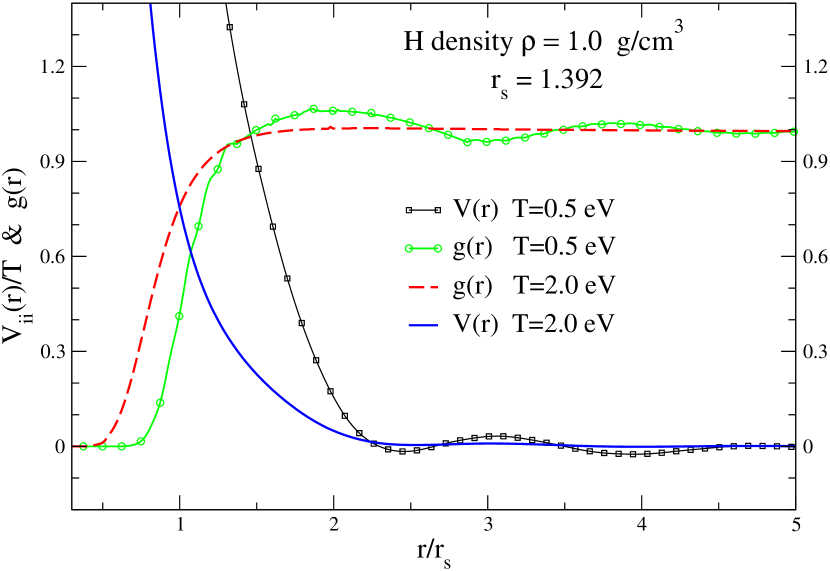
Figure 2: (Online color)The proton-proton pair potentials and PDFs at 0.5 eV and 2 eV in a Hydrogen plasma at $r_{s}$=1.391, with $\rho$=1.0 g/cm³, at $T$ significantly higher than a possible phase transition and contains protons and electrons.The pair-potentials contain Friedel oscillations whose minima line up with the peaks in the $g(r)$.

Quantum statistical potentials have also been considered for finite-$T$ electronic systems since the 1960s DunnBr67 ; Filinov04 , and more recently JonesMur07 , where the latter authors concluded that such methods treat many-body effects inadequately.

The point-ion model is unsatisfactory even for protons for $T<E_{F}$ as discussed below. The proton-proton pair-potential is a most demanding case for the NPA method because the charge pile up around the proton is highly non-linear, and the methods used here become inapplicable without further modification when very few free electrons are present, while partial ionizations strictly require the use of a mixture of ions of different ionizations. Forms like H^-, H, H⁺ as well as quasi-molecular transient forms like H${}_{2}^{+}$, may occur in H plasmas near a phase transition. The fully ionized case (i.e., a proton) has no bound core, and yet the point-ion model fails since a form factor associated with the non-linear charge pile up is needed. We find that the form factor from the NPA works with adequate accuracy, and even picks up the effects of transient H${}_{2}^{+}$ in the medium when relevant. We give an illustrative example below, using fully ionized hydrogen. Similar transients in hydrogen have been noted by Norman et al Norman17H .

Fig. 2 displays the the proton-proton pair potential and PDFs at 0.5 eV and 2 eV for a hydrogen plasma at $r_{s}\simeq 1.392$, $\rho=1.0$ g/cm³. The plasma is fully ionized, although close to a first-order transition from a molecular liquid to a conducting atomic fluid, believed to occur near $T\sim$ 0.13 eV. Nuclear quantum effects are also important near the phase transition. How they may be included in NPA models will be discussed elsewhere, following previous work based on the classical-map approach to quantum effects cdw-N-rep19 . Here we neglect them, working at a higher temperature of 0.5 eV and 2 eV. In Fig. 3 we display the D-D PDFs at a somewhat lower density where the tendency to form transient bonding is higher.

The broad hump in the $g(r)$ in Fig. 2 from 1.5$<r/r_{s}<2.5$ corresponds to the range of bond lengths associated with the presence of transient H${}_{2}^{+}$ states as well as with H⁺ packing effects. The peak due to purely packing effects occurs near $r/r_{\rm ws}\sim 1.6$. The nominal H${}_{2}^{+}$ bond length of $\simeq 2$ a.u. in a vacuum at $T=0$ is extended in a plasma due to screening and temperature effects. The bond becomes transient, with a broader range of lengths.

It should be noted that the NPA pair-potentials are very long-ranged, encompassing some tens of Wigner-Seitz radii. The aluminum pair-potential near its melting point requires using a pair-potential extending over at least a dozen atomic shells if the phonon spectra are to be accurately recovered HarbEOSPhn17 . This should be compared to those used in the pair-potential part of empirical models like the SW potential which extends to only about one Wigner-Seitz radius. The belief popular in the empirical modeling community that pair-potentials cannot reproduce tetrahedral structures without “three-body forces” is certainly true if the pair-potential does not even extent to the next-nearest neighbour (N-N-N) position!

The minima in the Friedel oscillations of the NPA potentials correspond approximately to shells of atoms where the third, fourth and higher neighbours are positioned, as seen by a comparison with the PDFs generated from these potentials. The PDFs are generated using the NPA potentials in classical MD, or in a hyper-netted-chain equation inclusive of a bridge term. Simulation methods for long-range potentials, viz,, Ewald constructions, use of analytic tails etc., are well known and pose no difficulties, even for extracting dynamic structure data using NPA potentials Nadin88 ; HarbourDSF18 .

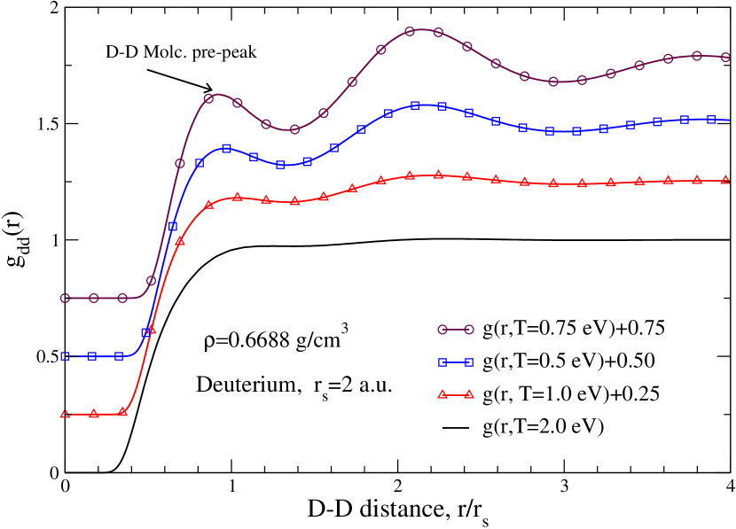
Figure 3: (Online color)The deuteron-deuteron pair distribution functions display the onset of transient D-D molecular forms (e.g., D${}_{2}^{+}$) as the temperature is lowered from 2 eV to 0.3 eV, for a deuterium plasma at $r_{s}=2$. The D⁺ are fully ionized and only transient molecular forms exist, while there are no atomic bound states.

A potential with wider applicability to uniform fluids than the Yukawa model is obtained using the random phase approximation (RPA) to the response function. This retains the all important Friedel oscillations in the pair potential for $T/E_{F}<1$. At high temperatures this reduces to the Vlasov approximation and then to the Yukawa form. The pair-potential, the detailed computations of the pair distribution functions (PDFs), free energies and EOS properties of a plasma of point charges interacting via the RPA screened Coulomb potential is an important reference point. These have been computed as a function of the plasma parameter $\Gamma=Z/(r_{ws}T)$ by Perrot Perrot91 . However, the assumption of negligible core size (point-ion approximation) is not adequate for most ions except at high $T$. Neither the RPA form, nor the Yukawa form, is designed to satisfy the compressibility sum rule.

A complete treatment of ion-ion interactions needs core-core interactions as well as the inclusion of a form factor in the electron-ion pseudopotential $U_{\rm a}^{ei}(k)$. We use Eq. 12, which is an accurate yet simple pseudopotential directly available from any average-atom calculation. We have successfully used the NPA $U^{ei}(k)$ in many diverse materials and WDM systems ranging from solid Be, Na, Al, to plasma states of Be, Li, C, Ga, Al, or Si even as a supercooled liquid.

The pseudopotential resulting from Eq. 12 is a simple local potential ($s$-wave potential). If the density displacement $a_{f}(k)$ is expanded in terms of the contributions from different angular momentum states $l$ of the Kohn-Sham eigenstates, then a non-local ($l$-dependent) pseudopotential can be constructed. Such non-local forms are needed in solid-state applications where spherical symmetry is lacking. However, the simple $s$-wave form given in Eq. 12 seems to work well for fluids, their EOS and static transport coefficients.

Aluminum is regarded as a ’difficult’ material by those who develop effective medium potentials for it. In Fig. 4 we display Al-Al pair potentials for several temperatures and compressions, including for a case where the ions are held at 1 eV, while the electrons are at 1 eV, or at 5 eV and 10 eV. The potentials show how the Friedel oscillations disappear at high electron temperatures. These minima, which determine the location of N-N, N-N-N positions bring in the multi-center features that empirical models like the SW potential put in “by hand”. However, Fig. 4 shows that the peaks and troughs in the $g(r)$ are not entirely determined by the pair potential as the ‘volume energy’ of the electron fluid plays a part, and largely determines the position of the first peak in high-$\bar{Z}$ systems like liquid aluminum or liquid carbon (see discussion in Ref. DWP-carb90 ).

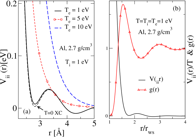
Figure 4: (Online color) (a)The Al-Al pair potentials at normal density from the NPA for WDMs in thermal equilibrium at $T=1$ eV, and two WDM states with $T_{e}\neq T_{i}$. The Fermi energy $E_{F}\sim 12$ eV, and the electron degeneracy changes. If the electron XC is treating using the $T=0$ instead of $T=1$ eV, there is a slight error in the depth of the first energy minimum. (b) The Al pair-potential at 1 eV (black line) and its g(r) are shown as a red line with triangles. The energy is scaled by $T$, and the position by $r_{\rm ws}$, unlike in the left panel. The first maximum in the g(r) is at a positive energy and not at the lowest minimum in the pair potential. It is the preferred first-neighbour position because the the XC-energy favours a denser electron fluid. The second and third neighbours, corresponding to the secondary peaks in the PDF are nearly at the Friedel minima.

The PDFs $g(r)$ can be obtained from the pair-potential either using classical MD, or using the modified HNC equation (MHNC). The $g(r)$ shown in Fig. 4(b) has been obtained using the MHNC and a Bridge term based on a hard sphere liquid with a packing fraction of 0.2996. It is also of interest to see how well these NPA PDFs of one-center DFT agree with direct simulations using an $N$-center DFT procedure like that of the VASP or ABINIT. In Fig. 5 we give comparisons of NPA for two PDFs with those of Recoules et al. recoules15 , with $N$=64 atoms in the simulation cell. The PDFs obtained from DFT-MD simulations are sensitive to the type of electron XC-functional used, and a higher $N$ is needed to get better statistics. However, the NPA $g(r)$ and the DFT-MD can be considered to be in good agreement.

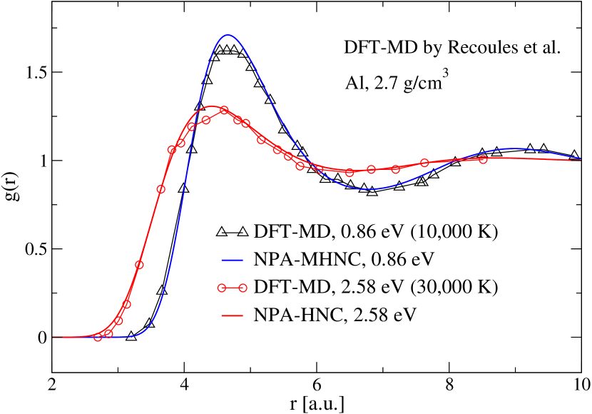
Figure 5: (Online color)The NPA $g(r)$ for aluminum at two temperatures are compared with the DFT-MD simulations of Recoules et al recoules15 . The simulations use 64 atoms and the PBE functional. Better agreement near the first peak is obtained from simulations with more atoms.

III.2 Contributions to the potential from the core-electron density

Equation  11 contains $V^{cc}$ and $V^{cf}$ where the core-electron density contributes to the pair-potential. In the following we show that the neglect of core-core interactions can lead to very serious differences, e.g., specially in weakly ionized plasmas containing neutral species.

The term $V^{cc}(r)$ contains $V(a_{c},b_{c})$ which is the interaction between the density distributions of the bound electron core in the atom ‘a’ with the core electrons in ‘b’. These are not the unperturbed NPA densities $n_{c}(r)$ defined in Eq. 9, but the densities that result from the perturbation of each density by the other, in the plasma environment. The unperturbed core density of the ion ‘a’ is denoted by $n^{0}_{c}(\vec{r}_{a}),\vec{r}_{a}=\vec{r}-\vec{R}_{a}$ and similarly for the ion ‘b’, with $R=|\vec{R}_{a}-\vec{R}_{b}|$ defining the scalar separation of the two atoms. The contribution to the pair-potential is:

$$V^{cc}(R) = Z_{a}Z_{b}/R+\int\frac{dr^{3}dr^{\prime 3}n^{0}_{c}(\vec{r}_{a})n^{0}_{c}(\vec{r^{\prime}}_{b})}{|\vec{r}-\vec{r}^{\prime}|}+$$ (22)

$$\Delta_{ES}(R)+\Delta_{xc}(R).$$

The potential contains an electrostatic correction $\Delta_{ES}(R)$ as the core densities are modified by the interaction. Instead of doing a two-center calculation for this term, second-order perturbation theory based on the polarisability of the core density is sufficient specially when there are free-electron screening effects, as in plasmas or metals. An electron XC-term $\Delta_{xc}(R)$ is associated with the density modification. This includes a correction to the kinetic energy functional as well as terms arising from XC-effects. That is, evaluating $\Delta_{xc}(R)$ accurately is somewhat complicated. A strictly density-functional approach is discussed in Appendix B of ref. eos95 .

A simplified approximate procedure is as follows. The core-core interaction can be written as a sum of monopole, dipole, quadrupole and higher terms. In systems with free electrons (e.g., plasmas), only the dipole term of the expansion is of importance due to screening effects. The frequency-dependent part of the dipole interactions brings in the van der Waals (vW) type of contributions known as “dispersion forces”. These have been discussed extensively within DFT Maggs87 ; Ber2015vWals . While they are easily included in the NPA approach, they are hard to include in the usual $N$-center DFT used in codes like the VASP because of their strong non-locality. One method used in $N$-center DFT calculations is to decompose the $N$-center charge density into $N$ individual charge distributions (each like an NPA). Using maximally localized Wannier functions on each atomic center together with a polarizability analysis for each center is one typical approach. The need for such procedures is an artifact of the usual $N$-center DFT approach where even a fluid is represented as an average over an ensemble of MD generated solids. The NPA scheme directly provides such single-center distributions in the appropriate form; hence dipole forces and vW effects are easily included when needed.

In practical WDM calculations where free electrons are present, the metallic interaction $V_{\rm ab}^{ff}(k)$, Eq. 17 is dominant. Then a fairly simple procedure may be sufficient for including core-core interactions when they become relevant. For instance, given an atom ‘a’ with an argon-like core, and an atom ‘b’ with a krypton-like core, we use the known Ar-Kr interaction given as a multipole expansion and screen it using the free-electron dielectric function of the WDM electrons at the appropriate free-electron density $\bar{n}$ and $T$.

We illustrated this using an example, namely, a mixture of neutral argon atoms Ar⁰, together with argon ions Ar${}^{Z_{i}+}$ with appropriate integer ionizations $Z_{i}$. In an argon plasma with, say, $\bar{Z}=0.3$ it is clear that most of the atoms ($\sim$ 70%) are neutral argon atoms, while some $\sim 30$% are singly ionized Ar⁺ ions. Treating such a system needs the neutral Ar-Ar interactions which are purely core-core interactions. We also have Ar-Ar⁺ as well as Ar⁺-Ar⁺ interactions, i.e., three pair-potentials and three ion-ion PDFs associated with them. A single average-atom NPA or a naive $N$-atom DFT calculation is quite inadequate for accurately estimating physical properties of such a system.

In evaluating physical properties of the Ar, Ar⁺ mixture, say, the self-diffusion coefficient, there are two self-diffusion coefficients, and one inter-diffusion coefficient as well. They are also constrained by the compressibility sum rule. In such instances, the meaning of the self-diffusion coefficient obtained from an $N$-center DFT calculation (e.g., a VASP calculation) needs to be examined more carefully in the context of partitioning the results to ascribe them to individual ionization species.

Evaluations of core-core potentials for neutral argon atoms in a medium without free electrons give results close to parameterized potentials similar to the Lennard-Jones(LJ) or more advanced rare-gas potentials. The presence of free electrons leads to screening of the core-core interaction. Thus, at the LJ-level of approximation, $V^{cc}(k)$ for two neutrals immersed in the appropriate electron gas is approximately given by $V^{LJ}(k)\{1+V_{k}\chi(k,T)\}$.

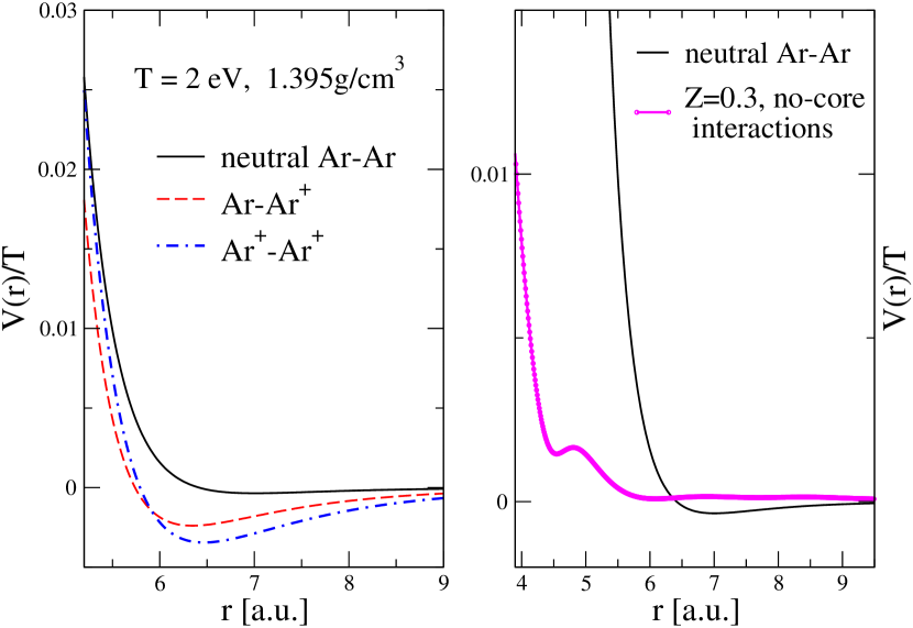
Figure 6: (Online color)The screened pair-potentials Ar-Ar, Ar-Ar⁺ Ar⁺-Ar⁺ of a two-component mixture of argon at 2 eV. The single Average-Atom pair-potential $V_{\rm a,a}^{ff}(r)$, a=Ar^0.3+ is obtained (thick magenta curve) for ions with $\bar{Z}$=0.3, without including core-core interactions

For two charged ions, the major interaction is via free electrons, and is given by the usual form, Eq. 17. The major part of the interaction between the ion and the neutral atom is the energy of the induced dipole of the neutral atom interacting with the electric field of the ion, moderated by screening. There is also a shell-shell repulsion, giving rise to a modified LJ-like potential. The polarizability and other parameters can be evaluated using the bound electron densities of the Ar atom and the Ar⁺ ion obtained from the respective NPA calculations, or using known LJ parametrizations. In Fig. 6 we display the three pair-potentials relevant to argon at normal density and $T=2$ eV, when $\bar{Z}=0.3$, and when treated as a mixture. However, if the system is treated as a single component fluid of average atoms with a charge of $\bar{Z}$=0.3, the resulting pair-potential evaluated without including core-core corrections is found to be quite different (right panel, Fig. 6) from those inclusive of core corrections.

III.3 The response function of the uniform electron fluid

The response function is itself a functional of the one-body electron density and can be evaluated self-consistently within the calculation by solving the NPA-Kohn Sham equation for just the central cavity but without a nucleus. Then the free electron density pile up $a_{f}(k)$ is entirely due to the cavity potential $V_{cav}(k)$ which is the electrostatic potential of a weak spherical cavity. Then Eq. 12 can be used in an inverse sense to calculate $\chi(q,T)$ in situ. While such an approach is useful as a control calculation, the following direct procedure has been implemented in our codes.

The interacting electron gas response function used in these calculations includes a local-field factor (LFC) chosen to satisfy the finite temperature electron-gas compressibility sum rule.

$$\chi(k,T) = \chi_{ee}(k,T_{e})=\frac{\chi_{0}(k,T_{e})}{1-V_{k}(1-G_{k})\chi_{0}(k,T_{e})},$$ (23)

$$G_{k} = (1-\kappa_{0}/\kappa)(k/k_{\text{TF}})^{2};\quad V_{k}=4\pi/k^{2},$$ (24)

$$k_{\text{TF}}/k_{F} = \{(4/\pi)\alpha r_{s})\}^{1/2};\quad\alpha=(4/9\pi)^{1/3},$$ (25)

$$V_{ii}(k) = Z^{2}V_{k}+|U_{ei}(k)|^{2}\chi_{ee}(k,T_{e}).$$ (26)

Here $\chi_{0}$ is the finite-$T$ Lindhard function, $V_{k}$ is the bare Coulomb potential, and $G_{k}$ is a local-field correction (LFC). The finite-$T$ compressibility sum rule for electrons is satisfied since $\kappa_{0}$ and $\kappa$ are the non-interacting and interacting electron compressibilities respectively, at the temperature $T$, with $\kappa$ matched to the $F_{xc}(T)$ used in the KS calculation. In Eq. 25, $k_{\text{TF}}$ appearing in the LFC is the Thomas-Fermi wavevector. We use a $G_{k}$ evaluated at $k\to 0$ for all $k$ instead of the more general $k$-dependent form (e.g., Eq. 50 in Ref. PDWXC ) since the $k$-dispersion in $G_{k}$ has negligible effect for the WDMs of this study.

IV The NPA pair-potential approach compared to methods based on multi-center potentials

The pair-potential $V_{\rm ab}(R)$ is normally understood as the energy of the system with two ‘atoms’, or ‘ions’ as the case may be (but referred to here as ‘atoms’) and denoted by ‘a’ and ‘b’ and held at a separation $R$ , compared to the limit $R\to\infty$ when there is no interaction between them. This has a clear meaning if the system is in a vacuum and at sufficiently low $T$ such that ‘a’ and ‘b’ remain as compact objects. Thus the ‘bond energy’ of two hydrogen atoms calculated using standard quantum chemistry methods, at $T=0$, has no ambiguity. However, in an atomic or molecular fluid, or in a WDM, the medium contains other atoms and even free electrons, with $T\neq 0$.

So one needs to include the effect of neighbouring atoms that are in the medium. This is exactly the problem systematically addressed by many-body theories like DFT. The effect of the medium is a functional of the one-body densities of the components that make up the medium where the two atoms ‘a’ and ‘b’ are placed in. Instead of constructing the necessary functionals in a systematic way, keeping in mind that they should be one-body functionals, semi-empirical potentials (fitted to data bases etc.) have deployed multi-center models mimicking bonds, bond angles, their torsional properties and so forth, based on preconceived ‘chemical bonding’ pictures. If this ‘fitting’ had been directed to constructing just the electron XC-functional, then we have the effort found in quantum chemistry, colourfully described as constructing a “Jacob’s Ladder”, where increasingly sophisticated electron XC-functionals are constructed for electronic systems placed in the potential of a finite number of nuclei, usually held fixed.

In the following we illustrate the DFT-NPA approach of using pair-potentials and XC-functionals by comparing it with the Stillinger-Weber (SW) model as a well-known example of a multi-center potential useful for tetrahedral materials, be they in solid, liquid or even WDM states like molten silicon or liquid carbon.

IV.1 The $N$-body energy in the Stillinger Weber model

We briefly recount the details of the SW model for the convenience of the reader. The quantity they model is the potential-energy function $\phi$ for $N$ identical interacting particles. SW write the potential for Si as:

$$\phi(1,2,\ldots,N)_{\rm sw}=\sum_{i<j}V_{2}(i,j)+\sum_{i<j<k}V_{3}(i,j,k).$$ (27)

A one-body term is not displayed as it represents external potentials. SW truncate their expansion in third order. The two-body term is written as the sum of a repulsive term $V^{re}$, and an attractive term $V^{at}$. An energy scale $\epsilon$ and a length scale $\sigma$ are introduced as in the Lennard-Jones potential. The three body term should possess translational and rotational symmetry, and contains the bond angle $\theta_{jik}$. The three-body terms $V_{3}$ sums over the neighbours $k$ of the pair $i,j$.

$$V_{2}{i,j} = V_{2}(r_{ij})=V^{re}(r_{ij})-V^{at}(r_{ij})$$ (28)

$$V_{3}(i,j,k) = U(r_{ij})U(r_{ik})(\cos\theta_{jik}+1/3)^{2}$$ (29)

$$+ U(r_{ji})U(r_{jk})(\cos\theta_{ijk}+1/3)^{2}$$ (30)

$$+ U(r_{ki})U(r_{kj})(\cos\theta_{ikj}+1/3)^{2}$$ (31)

$$V^{re}(r) = A\epsilon(B/x^{p})\exp\{1/(x-a)\}$$ (32)

$$V^{at}(r) = A\epsilon(1/x^{q})\exp\{1/(x-a)\}$$ (33)

$$U(r) = \sqrt{(}\lambda\epsilon)\exp\{\gamma/(x-a)\},\;x=r/\sigma.$$ (34)

Here the angular part, with the $\cos\theta_{jik}$ function contributes strongly in favour of pairs of bonds arising from the atom ‘$i$’ that conform to the tetrahedral configuration common in C, Si etc., at normal densities and temperatures. That is, structural features are built into the potential assuming the validity of specific structures. The sum of contributions to the three-body forces from an ensemble of SW-atoms tends to zero as the structure tends to tetrahedral bonding, while other possible structures become destabilized by an unfavourable three-body contribution. It is standard-writ in classical MD simulations that ‘three-body terms are necessary’ to stabilize the diamond structure, but true only in the sense that LJ-type short-ranged pair potentials fail. The SW model contains seven fit parameters, of which $q$ is set to zero in Eq. 28. All three pair-functions that make up the SW potential vanish at $r=\sigma a$, with $\sigma=3.959$ a.u., $a=1.80$ and $\epsilon=2.1682$ eV, i.e., 25,160K for Si SW85 . Currently, there is a plethora of SW potentials with somewhat different parameter fits but the basic idea has been to “fit a potential” to structure data incorporating models of bond stretching, bond bending etc., rather than using one-body DFT functionals.

In fig. 7 we compare the SW pair potential to the NPA pair-potential and the DFT-MD potential extracted from a simulation of 216 particles Remsing17 , using the SCAN functional SCAN13 that is most appropriate for systems with covalent bonding. The very demanding case of supercooled molten silicon at 1200K has been used for a comparison of the NPA and DFT-MD VASP simulations. We choose this case as a detailed account of NPA potentials for molten supercooled Si is given in Ref. cdwSi20 and in the supplemental material associated with it.

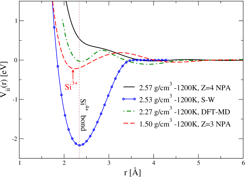
Figure 7: (color online) The pair-potentials from the NPA, from a VASP calculation with 216 atoms using the SCAN XC-functional for supercooled liquid silicon at 1200K, and at the metastable low density of 2.27g/cm³ are shown. The normal melt density is higher, being at 2.57 g/cm³ prevails above 1683K. The pair-potential for the unstable higher density liquid from NPA at 1200K is also shown. The Stillinger-Weber pair-potential for liquid Si at 1200K is contrasted with the other potentials. We also display the NPA potential for expanded molten Si at 1.5g/cm³ where a low-ionization state Si³⁺ occurs. The Si-Si nearest-neighbour “bond” distance is shortened for Si${}^{3}+$ ions, compared to the Si⁴⁺ pairs.

A ‘built-in’ feature of the pair part of the SW-potential is its deep negative energy near the Si⁴⁺ bond length in the solid. Such a deep feature is not found in DFT-VASP or in the DFT-NPA potentials. Unlike in SW containing only classical ions, the NPA and VASP calculations treat silicon as a two-component system with an ion subsystem and an electron subsystem. The stability of the system arises from the ionic interactions as well as a volume energy associated with the electron fluid. Hence the DFT models have a comparatively shallow ion-ion potential, while the SW potential has to be deeper to include the energy of the electron subsystem as a “bond energy” component. Furthermore, while a very short-ranged pair-potential alone is insufficient to ‘stabilize’ the one-component tetrahedral structure, a long-ranged pair-potential inclusive of the ‘electron gas’ contribution to the total energy covers all the possible electron-ion structures that are quantum mechanically possible. As already noted in discussing the potentials and PDFs of Al, Ar, hydrogen, and in previous publications on C, Si DWP-carb90 , Al cdw-aers83 , the energy minima in the Friedel oscillations of the ion-ion pair potential, together with the volume dependent energy effects of the electron fluid, were seen to correlate closely with the positions of the higher-order neighbours beyond the nearest neighbour.

A comparison of the Si-Si $g(r)$ obtained from various calculations is given in Fig. 8. The PDFs from NPA calculations, DFT-MD calculations using the SCAN XC-functional, as well as the PBE PBE96 XC-functional are shown, together with a typical classical MD simulation for the SW potential  YuSW96 . The SW potential is chosen here for comparison as it is superior to the Tersoff potential and other EMA potentials for modeling liquid-Si Cook-Si93 .

The differences between the one-center NPA with LDA, 216-atom DFT-MD with PBE, and with SCAN are similar in magnitude; comparison with experiment shows that none is superior to the other cdwSi20 . The one-center electron density distribution used in the NPA is very simple and smooth compared to the 216-center $n(r)$ used in the VASP calculation. In fact, the LDA-XC is generally found to work efficiently and accurately for the NPA. Furthermore, the NPA calculation with the hyper-netted-chain (HNC) equation is computationally much faster and cheaper than the SW simulation, while also being a first-principles DFT calculation.

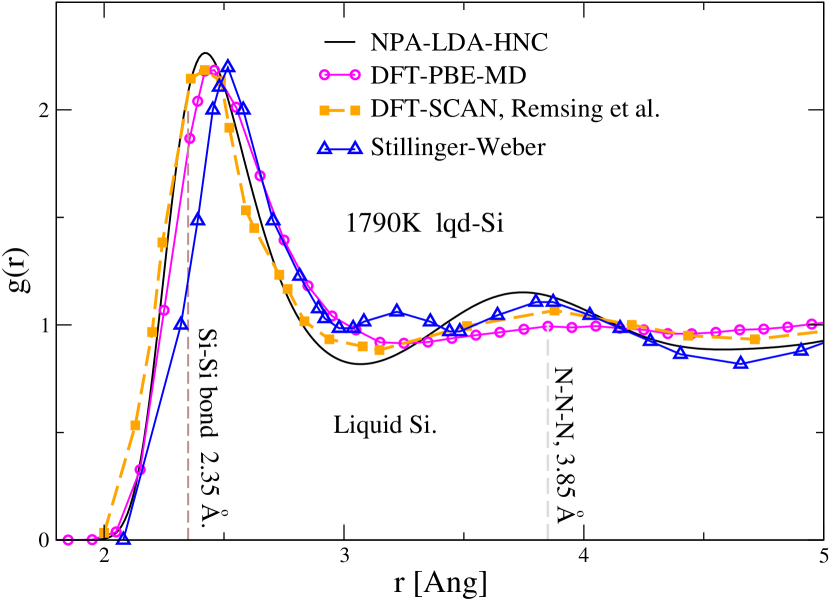
Figure 8: (Online color) The PDFs for molten Si slightly above the melting point calculated by several methods is displayed. Two DFT-MD calculations using the VASP, code, and with the SCAN and PBE XC-functionals show sensitivity to the functionals used in the 216 atom calculation. The NPA, using only one Si atom has a much smoother electron distribution and obtains comparable results with an LDA XC-functional. The indicated nearest-neighbour (N-N) and N-N-N distances are for solid Si. The S-W model shows a spurious hump near 3-3.5 Å .

IV.2 The ion-ion $N$-body corrections and the NPA model

It is of interest to see how the pair-potential used in the NPA brings in the three-body energy and such ‘multi-center’ terms via the ion-ion XC functional used in the NPA approach. Of course, if classical MD is used with the NPA pair-potentials Nadin88 ; HarbourDSF18 ; Stanek21 , then the ion-ion correlations are automatically built up by the long-range pair-potentials. Such simulations yield the $g_{ii}(r)$, but the calculation of the total free energy requires contributions from the electron subsystem to the total energy, as discussed in Ref. eos95 . In using the SW potential, the $g_{ii}(r)$ and the SW-potential are sufficient to determine the total energy as there is no electron subsystem.

Here we consider the question of many-ion effects using the theory of integral equations for ion correlations. In contrast to the SW-potential, the NPA pair potentials do not include any pre-assigned structural characteristics except for the effect of the average ion density imposed by the Wigner-Seitz sphere. SW-type pre-assigned structures are usually valid only in a specific regime of $\bar{Z}$ (e.g., carbon with a valance of four), $\bar{\rho}$. The pair-potentials and the associated XC-functionals of the NPA approach generate the appropriate lowest energy structure where the local ordering may be tetrahedral, face-centered etc., or a thermodynamic mixture of many structures with no predominant structure.

We consider a uniform fluid consisting of atoms of one type for simplicity. The DFT Eq. 4 for the ion subsytem solves for the minimum energy ion distribution $\rho(r)$ and gives the form:

$$\rho(r)=\bar{\rho}g(r)=\bar{\rho}\exp\{-V_{I}(r)/T\}.$$ (35)

where $V_{I}(r)$ is the density-functional potential felt by an ion $I$ at the radial location $r$, in the presence of an ion at the origin. This potential can be written within DFT as:

$$V_{I}(r) = V_{0I}(r)+V(\rm{mean\ field})+V_{ii}^{xc}(r)$$ (36)

$$V_{ii}^{xc} = V_{ii}^{c}(r)=\delta F_{ii}^{xc}[\rho(r),n(r)]/\delta\rho(r).$$ (37)

The first term on the r.h.s., $V_{0I}$ is the ion-ion pair potential between the central ion at the origin and the ion $I$ at $r$, viz., the NPA pair-potential. Any arbitrary ion is denoted by the lower-case $i$. The ion $I$ is also subject to the self-consistent average potential at $r$ from all the field ions in the medium, i.e., from the density $\rho(r)=\bar{\rho}g(r)$. The effect of the electron distribution $n(r)$ has to be included in the mean-field potential. The relevant electron density is that given by the solution of the Kohn-Sham equation, viz., Eq. 3, coupled to the ion density. Then the mean-field potential is just the Poisson potential. when evaluated at the level of a monopole expansion, i.e., neglecting core effects and pseudopotential form factors. Defining the convolution integral by

$$f*g=\int d\vec{r}_{1}f(r_{1})g(|\vec{r}-\vec{r}_{1}|),$$ (38)

the Poisson potential is given by

$$\bar{Z}\{\rho-n\}*\{V\},\;V(r)=\bar{Z}/r.$$ (39)

Terms not contained in the mean-field are in the ionic-XC term $V_{ii}^{xc}(r)$. We also neglect electron-ion XC effects and use the Born-Oppenheimer approximation (see Ref. ilciacco93 ). Since ions are classical, there is no exchange, and this is purely a correlation term that can be calculated using classical statistical mechanics.

The ion correlation free energy is formally given as a coupling-constant integration on the $g_{ii}(r)$ eos95 , just as for the electron XC-functional. But $g_{ii}(r)$ is initially unknown. An LDA $V_{ii}^{c}(r)$ based on the classical correlation energy of the uniform classical Coulomb fluid, similar to the LDA for electron correlations fails, as reported in Ref. DWP1 . It is found that $V_{ii}^{c}(r)$ is highly nonlocal and even gradient expansions fail. Hence we exploit the relationship of the XC-functional with the corresponding pair-distribution functions as follows.

The three-body and higher correlations neglected in the mean-field potential are included via the Ornstein-Zernike relation which expresses the total correlation function $h(r)=g(r)-1$ in terms of the direct correlation function $c(r)$. We write the Ornstein-Zernike equation as:

$$h_{ii}(r_{12})=c_{ii}(r_{12})+\bar{\rho}c_{ii}(r_{13})*h_{ii}(r_{31}).$$ (40)

This equation is a simple algebraic equation in $k$-space for fluids of uniform-density. It brings in the interaction of the two atoms $1,2$ with all possible ‘third atoms’ at the location $\vec{r}_{3}$ which runs over all space. The explicit correlation corrections are selected to be the sum of hyper-netted-chain (HNC) diagrams excluding mean-field terms that have already been taken into account in Eq. 36. That is, noting that $r$=$|\vec{r}_{12}|$ in the uniform case, and using the short-ranged direct correlation function $\tilde{c}_{ii}(r_{12})$ we have

$$V_{ii}^{c}(r)/T = -\bar{\rho}\,\tilde{c}_{ii}*h_{ii}$$ (41)

$$\tilde{c}_{ii}(r_{)} = c_{ii}(r)+V_{I}(r)/T.$$ (42)

Classical correlations not captured by the HNC sum are not easily evaluated and are bundled into a ‘bridge diagram’ evaluated using hard-sphere models LFA83 .

In actual NPA calculations where a large correlation sphere of radius $R_{c}$ is used, all quantities are referred to the limit $r\to R_{c}$. This is true for all XC-potentials as well as other quantities like chemical potentials. That is, $V_{ss^{\prime}}^{xc}(r)$ are effective values $V_{ss^{\prime}}^{xc}-V_{ss^{\prime}}^{xc}(R_{c})$.

IV.3 Expressions for total Free energy in the NPA model

For comparison with expressions to be given below for effective medium theories, we discuss the total Helmholtz free energy $F$ of a fluid of neutral pesudoatoms. The evaluation of the free energy is more complicated than that of the internal energy $E_{tot}$, as calculations of the entropy contribution to $F$ in DFT is not conceptually straightforward especially in dealing with atomic bound states with partial occupancies. The total free energy per atom for a given ionic configuration (expressed as the density distribution $\rho(r)=\bar{\rho}g(r)$ around a given nucleus) is schematically summarized below, while the full expressions may be found in Refs. Pe-Be and eos95 .

$$F = F_{id}+F_{0}+F_{em}+F_{12}-E^{0}_{at}$$ (43)

$$F_{0} = \bar{Z}f^{h}(\bar{n},T)=\bar{Z}(f_{k.e}+f_{xc})$$ (44)

$$F_{em} = \Delta F_{0}+\Delta V_{ei}(\Delta n)+\Delta V_{ee}(\Delta n\Delta n^{\prime})$$ (45)

$$F_{12} = (1/2)\sum^{\prime}_{j}V_{12}(R_{j})+\mbox{cavity \ corrections}.$$ (46)

The energy of an isolated atom at $T=0$ in its ground state, $E^{0}_{at}$, is used as the reference energy. Here $F_{id}$ is the classical ideal-gas energy of the non-interacting ion subsystem per atom. Each atom contributes $\bar{Z}$ free electrons to the electron fluid. $F_{0}$ is the free energy of $\bar{Z}$ electrons in a uniform electron gas, $f^{h}$ the homogeneous free energy/electron, containing a kinetic energy component and an XC-component. The “embedding free energy” of a neutral pseudo atom is $F_{em}$. This is defined as the difference between the free energy of the electron fluid of mean density $\bar{n}$ with and without the NPA. It consists of a correction to $F_{0}$, the Coulomb interaction of the pseudo-ion with the displaced electrons, as well as the correction to the electron-electron repulsion energy due to the displaced electrons.

The $F_{12}$ term contains the free energy contributed through the ion-ion pair-distribution function and the pair-potential. The many-atom correlations dependent on the ‘environment’ are included here via the ion-ion PDF. Hence this is effectively the pair-energy and the correlation corrections to the free energy of the classical ions. That is, in more conventional language, the ‘bonding energy’ of two ions immersed in the fluid with average densities $\bar{n}$ and $\bar{\rho}$, inclusive of the effect of their higher-order neighbours brought in via the secondary peaks of the PDFs.

While $F_{0}$ is a smooth function of the electron density, sharp jumps may occur in $F_{12}$, and to a lesser extent in $F_{em}$, signaling the onset of ionization changes, structural changes or phase transitions. Example of such discontinuities at liquid-liquid phase transitions (LPT) may be found in Ref. cdwSi20 for liquid Si, while similar transitions have been noted in theoretical studies of liquid carbon as well glosli99 ; CPP-carb18 . Interestingly, a molten-carbon LPT was predicted in Ref. glosli99 using an empirical bond-order multi-center carbon potential, but this was not confirmed when DFT-MD simulations were done using the PBE functional WuLPT02

V effective medium potentials and NPA potentials

Unlike the purely classical SW model and effective medium approach (EMA), embedded-atom models (EAM) pay attention to the existence of an electron subsystem, and begin by using approximations to $T=0$ DFT to include the “effect of the local environment” of an ion in the medium. The Finnis-Sinclair potentials FinisSinc84 used in metallurgical applications is based on a second-moment approximation to tight-binding but reduces to an effective-medium type approach. A DFT type discussion is used in the initial theory of effective media to justify the use of a form of the total energy which is then parameterized using a variety of empirical models containing fit parameters. Hence systematic generalizations for $T\sim E_{F}$ or higher $T$ are not available although low-$T$ fitted forms exist. Here we examine the more systematic foundations which are, however, of little use in evaluating many of the current models which should be regarded as sophisticated empirical fits to data bases.

The total energy of the electron-ion system is written in EMA as:

$$E_{tot}=\sum_{i}F\{n_{i}(\vec{R}_{i})\}+(1/2)\sum_{i,j}\phi(\vec{R}_{i}-\vec{R}_{j}).$$ (47)

Here $F\{n_{i}(\vec{R}_{i})\}$ is a function of the electron density, with $n_{i}(\vec{R}_{i})$ being electron densities at atomic sites $\vec{R}_{i}$. Also, $\phi(\vec{R}_{i}-\vec{R}_{j})$ is a pair-potential mainly used to model the repulsive interactions among the atoms. The atomic densities are associated with an embedding energy which is taken to be a function of the local average one-body electron density $\bar{n}$, following DFT. The embedding energy at $T=0$ as a function of the electron density has been tabulated by various authors, e.g., Stott et al StottZaremba85 . A superposition approximation is introduced, and the total energy is finally expressed as a sum of terms for the isolated-atom energies plus the embedding energy in the homogeneous electron gas, and a gradient expansion in the electron density is used to allow for the density changes at atomic sites. No attempt has been made to take advantage of ion-DFT using an ion-correlation functional.

However, this approach turns out to be inadequate in many ways, yielding wrong elastic constants etc DawBaskes84 . The embedded atom model (EAM) was a numerical improvement on the EMA. The EAM attempts to merely use the structure of the energy expression for fitting to parameterized forms similar to it. Below we consider a more sophisticated form known as the ‘glue model’ Ercolessi94 .

The parameter-free first-principles NPA pair-potential for Aluminum is compared with one of the original force-matched Al ‘glue’ potentials that uses some 40 fit parameters and some 32 constraints. The ‘glue’ model uses the form:

$$E_{tot}=\sum_{i}U\{\sum_{j}n(r_{ij})\}+(1/2)\sum_{i,j}\phi(r_{ij}).$$ (48)

Here, instead of the electron gas term used in the EMA, or in the NPA as given by Eq. 43, a ‘glue’ function $U(n)$ is used, while $\phi(r)$ denotes the pair-potential. Hence, this aluminum potential depends on specifying three functions, $\phi(r),n(r)$ and $U(n(r))$ that contain fit parameters and constraints. Here again, simplification of the problem that could be achieved using a DFT ion-correlation functional to include many-ion effects is not invoked. The forces obtained from this potential (defined in terms of parameters contained in polynomials or Padé forms or other fit functions) are matched (by adjusting the fit parameters) to those from first principles calculations for a large variety of atomic configurations and physical situations (solids, liquids, clusters, surfaces, defects etc.), including those at finite $T$. The Al potential of Ercolessi et al. has been fitted to liquid Al simulations at 1000K and 2200K (i.e., $T/E_{F}=0.016$).

The NPA approach has no fit parameters, and finds WDM states of Aluminum to be ‘easy’ systems for successful theoretical predictions. However, Al is regarded as as a ‘difficult case’ for effective medium methods. Many of the EAM potentials give poor predictions of aluminum melting temperatures, vacancy migration energies, diffusion constants, stacking fault energies, surface energies, phonon spectra and so forth. The NPA potentials have been tested mainly in WDM situations where they are in excellent agreement with DFT-MD calculations of EOS properties, PDFs, as well as for transport properties like the electrical conductivity cond3-17 and diffusion constants Stanek21 . Unlike the EAM, the NPA provides pseudopotentials and eigenfunctions needed for many other calculations, e.g., linear transport coefficients, line broadening, XRTS spectroscopy and energy relaxation elrDW01 .

A key difference between these fitted-potential approaches, and that of the NPA, is the inclusion of environment-specific features in the NPA, be it for a liquid or a solid, via the pair-distribution function $g(r)$ of the ionic structure appearing in the ion-correlation functional of the NPA, viz., Eq. 41. The needed $g(r)$ is generated in situ for fluids. In the case of specific crystal structures at low $T$, one can use a known explicit form, as in Perrot’s Be calculations Pe-Be , or the phonon calculations of Harbour et al HarbEOSPhn17 using the NPA.

In Fig. 9 we compare the NPA Al-Al pair potential with that of the ‘glue potential’ of Ref. Ercolessi94 . In panel (a) we display the NPA pair potential, labeled NPA2, for liquid aluminum at the normal density of 2.7 g/cm³ and $T$=2200K. The pair part of the glue potential is also shown (curve with triangles). Unlike in the case of the SW potential, the glue potential has Friedel like oscillations, although not as long-ranged as in the NPA2 potential. The force-matching methods do not usually have the accuracy to recover the weaker Friedel oscillations which decay as $1/r^{3}$. The additional term of the glue potential, i.e, $U(n)$ (not displayed in the figure) brings in contributions to the total energy that are also included in the NPA via the electron-fluid term and the XC-correlation energies of ions as well as electrons, as indicated in Eq. 43. The ion-correlation energy is structure dependent, as indicated in Eq. 41.

In Fig. 9 we also consider the case of Aluminum at a density of 6.264 g/cm³, and at a temperature of 1.75 eV. This corresponds to $T/E_{F}=0.086$ as $\bar{Z}=3$ for Aluminum even at this temperature and compression. The compression drives up the Fermi energy and the effective temperature $T/E_{F}$ remains low and the electrons are highly degenerate. The system has been studied experimentally and theoretically by Fletcher et al. Flet-Al-15 using a physically motivated ad hoc potential (YSRR6) Wunsch09 shown as a red dashed line. The YSRR potential is made up of a Yukawa (Y) potential and a short-ranged repulsive (SRR) potential. The YSRR6 potential at the density of 6.24g/cm³ had been fitted to the DFT-MD $g(r)$, and the corresponding $S(k)$ is shown as a red-dashed line in panel (b).

The first-principles potential from the NPA at this density and temperature is labeled NPA6. It is very different (black solid line) from the YSRR potential, but gives excellent agreement with the MD-DFT $S(k)$ as well as with the XRTS data of Fletcher, without any fitting. That many potentials produce only a few crystal structures or very similar liquid structures, and hence the inverse problem is open to much uncertainty is well established chenlai92 . However, the spurious candidates for the potential can be eliminated by their failure to predict other physical properties. The YSRR potential predicts a very low compressibility, very stiff phonon spectra, as well as unrealistic electrical conductivities, as discussed in detail by Harbour et al xrt-Harb16 . These emphasize the fact that fitting to a structural feature (or even several) is no guarantee of having approximated the physically correct potential.

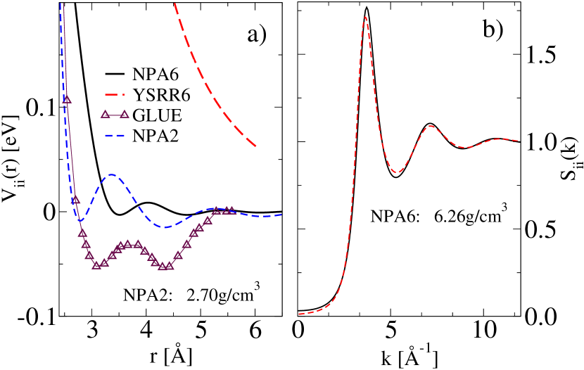
Figure 9: (Online color) Panel (a) displays the first-principles pair potential form NPA labeled NPA2 (blue dashed line) at $T$=2200K and the normal Al density of 2.7g/cm³, as well as the pair part of the ‘glue’ potential (triangles) of Ercolessi et al. NPA6 is the pair-potential for compressed Al at a density of 6.26 g/cm³ and $T$=1.75 eV studied experimentally by Fletcher et al Flet-Al-15 . A model potential (a Yukawa potential added to an ad hoc short-ranged repulsive potential) labeled YSRR6 used by Fletcher et al. is also shown (red dashed lines). In panel (b) the structure factors from the NPA6 potential and the YSRR6 potential are displayed. The YSRR6 potential reproduces the experimental $S(k)$ as it has been fitted to its $g(r)$. The NPA6 is a first principles calculation with no fit parameters xrt-Harb16 .

VI Discussion

The idea of using an ion correlation functional for treating ion-ion many body effects in ion-electron systems was proposed as early as 1982 DWP1 . It was motivated by the success of using an electron XC-functional to treat electron many-body effects. The method leads to a theory based on a pseudoatom, but it has not found significant adoption, partly because materials science has been mostly concerned with treating materials-science problems involving defects, dislocations etc., or with complex materials. Similarly, the idea of an ion correlation functional is of not much use for molecules and other finite systems used in quantum chemistry.

However, there is little excuse for not using pseudo-atom approaches for uniform systems at finite-$T$ as the conceptual and computational advantages are very significant.

A common misconception, partly arsing from the ‘chemical picture’ of bonding as the basis of complex correlations, as well as the wish to subsume the electron subsystem in bonds, has lead to the belief that the NPA “one-atom” approaches do not contain, and cannot include, many-ion effects associated with the local structure of the medium. Here we have given examples showing how the NPA calculations incorporate such effects, and clarified the kinship of the NPA approach and its energy functionals to those used in effective medium models. The NPA remains a strictly first-principles DFT approach, while the EMA approaches have now become largely spring boards for data fitting. The ability of the NPA to study subtle effects like liquid-liquid phase transitions in complex materials like liquid Si and liquid C has been demonstrated and these have been reviewed in the context of how ion correlations are included in the NPA pair-potential scheme. However, much of the success of the NPA depends on the existence of free electrons in the system that weaken the interparticle interactions. Additional steps are needed in treating weakly ionized systems and transition metals at very low temperatures.

Furthermore, although much effort has been directed to constructing kinetic energy functionals in the hope of simplifying DFT calculations, such calculations for $N$-atom systems will also not directly yield useful ‘one-atom’ properties like $\bar{Z}$, fractional compositions of ionic species, pseudopotentials and pair-potentials that are valuable intermediates for additional calculations of physical properties. In contrast, the NPA method provides such quantities directly, and may also easily include effects like van der Waals energies, and quantum nuclear corrections in its potentials.

VII conclusion

The NPA method has been successfully applied to a variety of warm-dense-matter systems, as well as to a number of solid-state systems. The detailed study of Si for supercooled and hot liquid silicon has shown that its accuracy is similar to DFT-MD simulations that may themselves differ from each other at the level of the electron XC-functionals used. The NPA, with its simpler one-body electron densities allows the use of the local density approximation in the XC functional. The NPA yields one-atom properties like the ionization state, fractional compositions of ionic species, pseudopotentials etc., not directly available from the $N$-atom VASP-type simulations. On the other hand, the NPA being a static DFT theory, does not provide the complex bonding structure that may prevail transiently in short-time scales. The thermodynamic properties of the system do not depend on such transient effects, and the NPA deals only with long-time averages.

DATA AVAILABILITY

All the data used in this paper are available within the article in graphical form in the figures 1 to 9. If there is any difficulty in extracting them from the figures, the data can be provided on request from the author.

References

- (1) E. K. U. Gross, and R. M. Dreizler, Density Functional Theory, NATO ASI series, 337, 625 Plenum Press, New York (1993).
- (2) M. W. C. Dharma-wardana, Phys. Rev. B 100, 155143 (2019) DOI: 10.1103/PhysRevB.100.155143
- (3) M. W. C. Dharma-wardana, D. Neilson and F. M. Peeters Phys. Rev. B 99, 035303 (2019) https://link.aps.org/doi/10.1103/PhysRevB.99.035303 DOI:10.1103/PhysRevB.99.035303
- (4) M. W. C. Dharma-wardana and F. Perrot Phys. Rev. B vol 70, 035308 (2004).
- (5) M.S.Daw, S.M. Foiles and M.I. Baskes, 9, 251-310 (1993).
- (6) F.H. Stillinger and T. A Weber, Phys. Rev. B 31, 5262-5271 (1985).
- (7) J. Tersoff, Phys. Rev. B 38 9902-9905 (1988).
- (8) Luca M. Ghiringhelli, Jan H. Los, A. Fasolino, and Evert Jan Meijer, Phys. Rev. B 72, 214103, (2005).
- (9) J. E. Saal, S. Kirklin, M. Aykol, B. Meredig, C. Wolverton, JOM 65, 1501 (2013).
- (10) S. Plimpton, Fast parallel algorithms for short-range molecular-dynamics, J. Comput. Phys. 117, 1-19 (1995).
- (11) S. Hamel, Lorin X. Benedict, Peter M. Celliers, M. A. Barrios, T. R. Boehly, G. W. Collins, Tilo Döppner, J. H. Eggert, D. R. Farley, D. G. Hicks, J. L. Kline, A. Lazicki, S. LePape, A. J. Mackinnon, J. D. Moody, H. F. Robey, Eric Schwegler, and Philip A. Sterne, Phys. Rev. B 86, 094113 (2012).
- (12) D. Kraus, Vorberger, D. O. Gericke, V. Bagnoud, A. Blazevic, W. Cayzac, A. Frank, G. Gregori, A. Ortner, A. Otten, F. Roth, G. Schaumann, D. Schumacher, K. Siegenthaler, F. Wagner, K. Wunsch, and M. Roth, Phys. Rev. Let. 111, 255501 (2013).
- (13) J. N. Glosli and F. H. Ree, Phys. Rev. Lett. 82, 4659 (1999).
- (14) Christine J. Wu, James N. Glosli, Giulia Galli, and Francis H. Ree, Phys. Rev. Lett. 89, 135701 (2002).
- (15) X.Gonze and C. Lee, Computer Phys. Commun. 180, 2582-2615 (2009).
- (16) G. Kresse and J. Furthmüller, Phys. Rev. B 54, 11169 (1996).
- (17) R. Evans, Adv. Phys. 28, 143 (1979).
- (18) K-U Plageman, H. R. Rüter, T. Bornath, Mohammed Shihab, Michael P. Desjarlais, C. Fortmann, S. Glenzer, R. Redmer, Phys. Rev. E 92, 013103 (2015).
- (19) Mandy Bethkenhagen, Bastian B. L. Witte, Maximilian Schörner, Gerd Röpke, Tilo Döppner, Dominik Kraus, Siegfried H. Glenzer, Philip A. Sterne, and Ronald Redmer, Phys. Rev. Research 2, 023260 (2020).
- (20) Valentin V. Karasiev, James Dufty, S.B. Trickey, Phys. Rev. Let. 120, 076401 (2018).
- (21) M.W.C. Dharma-wardana, Dennis D. Klug, and Richard C. Remsing. Phys. Rev. Lett. 125, 075702 (2020). doi: 10.1103/PhysRevLett.125.075702
- (22) M. W. C. Dharma-wardana, Contrib. Plasma Phys. 58 128-142 (2018).
- (23) M. W. C. Dharma-wardana and F. Perrot, Phys. Rev. Lett., 65, 76 (1990).
- (24) F. Perrot and M.W.C. Dharma-wardana, Phys. Rev. E. 52, 5352 (1995).
- (25) Olivier Hardouin Duparc, Philosophical Magazine Volume 89, 3117-3131 (2009).
- (26) M.W.C. Dharma-wardana in Laser Interactions with Atoms, Solids, and Plasmas, Carg’ese NATO workshop, 1992, Edited by R.M. More (Plenum, New York, 1994), p311.
- (27) L Harbour, and G. D. Förster, M. W. C. Dharma-wardana and Laurent J.Lewis, Physical review E 97,043210 (2018).
- (28) Lucas J. Stanek, Raymond C. Clay III, M.W.C. Dharma-wardana, Mitchell A. Wood, Kristian R.C. Beckwith, Michael S. Murillo, Phys. Plasmas 28, 032706 (2021). https://arxiv.org/abs/2012.06451
- (29) John Ziman, Proc. Phys. Soc 91, 701 (1967).
- (30) L. Dagens, J. Phys. C: Solid State Physics, 5, 2333 (1972).
- (31) F. Perrot, Phys. Rev. E 47, 570 (1993).
- (32) L. Harbour, M. W. C. Dharmawardana, D. D. Klug, L. J. Lewis, Phys. Rev. E 95, 043201 (2017).
- (33) M. W. C. Dharma-wardana and F. Perrot, Phys. Rev. A 26, 2096 (1982)
- (34) P.A. Sterne S.B. Hansen, B.G. Wilson, W.A. Isaacs, HEDP, 3, 278 (2007).
- (35) B. Rosznayi, High Energy Density Physics 4 64, (2008).
- (36) Gŕald Faussurier, Christophe Blancard, Philippe Cossé, and Patrick Renaudin Physics of Plasmas 17, 052707 (2010).
- (37) R. Piron and T. Blenski, Phys. Rev. E 83, 026403 (2011).
- (38) M. S. Murillo, Jon Weisheit, Stephanie B. Hansen, and M. W. C. Dharma-wardana, Phys. Rev. E 87, 063113 (2013).
- (39) C. E. Starrett, D. Saumon, J. Daligault, and S. Hamel Phys. Rev. E 90, 033110 (2014).
- (40) Yong Hou, Yongsheng Fu, Richard Bredow, Dongdong Kang, Ronald Redmer, Jianmin Yuan, High Energy density Physics 22 (2017) 21-26
- (41) J. P. Perdew, K. Burke, and M. Ernzerhof, Phys. Rev. Lett. 77, 3865 (1996).
- (42) J. Sun, B. Xiao, Y. Fang, R. Haunschild, P. Hao, A. Ruzsinszky, G. I. Csonka, G. E. Scuseria, and J. P. Perdew, Phys. Rev. Lett. 111, 106401 (2013).
- (43) F. Perrot and M. W. C. Dharma-wardana, Phys. Rev. B 62, 16536 (2000); Erratum: 67, 79901 (2003); arXive-1602.04734 (2016).
- (44) Richard C. Remsing, Michael L. Klein and Jianwei Sun, Physical Review B 96 024203 (2017).
- (45) M. W. C. Dharma-wardana, Contr. Plasma Phys, 55, 85 (2015).
- (46) F. Lado, S. M. Foiles and N. W. Ashcroft, Phys. Rev. A 26, 2374 (1983).
- (47) L Li, R. G. Parr, The Journal of chemical physics, 84, 1704 (1986).
- (48) E. Francisco, A. Martin Pendás, and M. A. Blanco J. Chem. Theory Comput. 2, 90?102 (2006).
- (49) P. R. Smy, Advances in Physics, 25 (5), 517-553, (1976).
- (50) S. H. Glenzer and Ronald Redmer, Rev. Mod. Phys. 81 1625 (2009).
- (51) M. W. C. Dharma-wardana, Phys. Rev. E 86, 036407 (2012).
- (52) F. J. Rogers, H. C. Graboske Jr., and D. J. Harwood, Phys. Rev. A 1, 1577 (1970).
- (53) L. G. Stanton and M. S. Murillo, Phys. Rev. E 93, 043203 (2016).
- (54) James P. Edwards, Urs Gerber, Christian Schubert, Maria A. Trejo, Axel Weber Progress of Theoretical and Experimental Physics, 2017 (8), 083A01 (2017).
- (55) H.Y. Sun, Dongdong Kang, Yong Hou, J.Y. Dai Matter Radiat. Extremes 2, 287 (2017).
- (56) T. Dunn, A.A. Broyles, Phys. Rev. 157, 156 (1967)
- (57) A. V. Filinov, V. O. Golubnychiy, M. Bonitz, W. Ebeling, and J. W. Dufty, Phys. Rev. E 70, 046411 (2004).
- (58) C.S. Jones, M.S. Murillo, High Energy Density Physics 3, 379-394 (2007)
- (59) G. E. Norman and I. M. Saitov, Doklady Physics, 2017, 62(6), 284-288 (2017) Original Russian Text, Doklady Akademii Nauk, 2017, 474(5), 553-557(2017).
- (60) F. Perrot, Phys. Rev. A 44, 8334 (1991).
- (61) V. Recoules, J. Bouchet, M. Torrent, and S. Mazevet, Rapport: Ab Initio calculations of X-ray Absorption. Spectra for warm dense matter, CEA, Arpajon, France (2015).
- (62) A. C. Maggs and N. W. Ashcroft, Phys. Rev. Lett. 59, 113 (1987).
- (63) K. Berland, V. R. Cooper, K. Lee, E. Schr‘ödee, T. Thonhauser, P. Hyldgaard, B. I. Lundqvist. Rep. Prog. Phys. 78 (6), 066501 (2015).
- (64) M.W.C. Dharma-wardana and G.C. Aers, Phys. Rev. B. 28, 1701 (1983).
- (65) W. Yu, Z. Q. Wang, and D. Stroud, Phys. Rev. B 54, 13946 (1996).
- (66) Stephen J. Cook and Paulette Clancy, Phys. Rev. B 47, 7686 (1993)
- (67) F. Nadin, G. Jacucci and M.W.C. Dharma-wardana, Phys. Rev. A 37, 1025-1028 (1988), [NRCC 2830].
- (68) Murray S. Daw and M. I. Baskes, Phys. Rev. B 29, 6443 (1994).
- (69) M. Finnis, J. Sinclair, Philosophical Magazine A 50 45 (1984).
- (70) M. Stott, E. Zaremba, Canadian Journal of Physics 60 1145 (1985).
- (71) F. Ercolessi and J. B. Adams, Europhysics Letters, 26, 583 (1994).
- (72) M.W.C. Dharma-wardana, D. D. Klug, L. Harbour, Laurent J. Lewis, Phys. Rev. E 96, 053206 (2017).
- (73) M. W. C. Dharma-wardana, Phys. Rev. E, 64 035401 (2001).
- (74) L. B. Fletcher, H. J. Lee, T. Döppner, E. Galtier, B. Nagler, P. Heimann, C. Fortmann, S. LePape, T. Ma, M. Millot, A. Pak, D. Turnbull, D. A. Chapman, D. O. Gericke, J. Vorberger, T. White, G. Gregori, M. Wei, B. Barbre, R. W. Falcone, C.-C. Kao , H. Nuhn, J. Welch, U. Zastrau, P. Neumayer, J. B. Hastings and S. H. Glenzer, Nature Photonics 9, 274 (2015).
- (75) K. Wünsch, J. Vorberger, and D. O. Gericke, Phys. Rev. E 79, 010201 (2009).
- (76) H. C. Chen and S. K. Lai, Phys. Rev. A 45, 3831 (1992).
- (77) L. Harbour, M. W. C. Dharma-wardana, D. Klug and L. Lewis, Physical Review E 94, 053211, (2016).