Origin of eclipsing time variations: Contributions of different modes of the dynamo-generated magnetic field

Abstract

Context. The possibility to detect circumbinary planets and to study stellar magnetic fields through eclipsing time variations (ETVs) in binary stars has sparked an increase of interest in this area of research.

Aims. We revisit the connection between stellar magnetic fields and the gravitational quadrupole moment $Q_{xx}$ and compare different dynamo-generated ETV models with our simulations.

Methods. We present magnetohydrodynamical simulations of solar mass stars with rotation periods of 8.3, 1.2, and 0.8 days and perform a detailed analysis of the magnetic and quadrupole moment using spherical harmonic decomposition.

Results. The extrema of $Q_{xx}$ are associated with changes in the magnetic field structure. This is evident in the simulation with a rotation period of 1.2 days. Its magnetic field has a more complex behavior than in the other models, as the large-scale nonaxisymmetric field dominates throughout the simulation and the axisymmetric component is predominantly hemispheric. This triggers variations in the density field that follow the magnetic field asymmetry with respect to the equator, affecting the $zz$ component of the inertia tensor, and thus modulating $Q_{xx}$. The magnetic fields of the two other runs are less variable in time and more symmetric with respect to the equator, such that the variations in the density are weaker, and therefore only small variations in $Q_{xx}$ are seen.

Conclusions. If interpreted via the classical Applegate mechanism (tidal locking), the quadrupole moment variations obtained in the current simulations are about two orders of magnitude below those deduced from observations of post-common-envelope binaries. However, if no tidal locking is assumed, our results are compatible with the observed ETVs.

1 Introduction

Post-common-envelope binaries (PCEBs) are commonly composed of a white dwarf and a low-mass main-sequence star. Observations of eclipses in these systems reveal deviations from the calculated eclipsing times in approximately $90\%$ of these systems (Zorotovic & Schreiber, 2013), with binary period variations on the order of $10^{-6}\ldots 10^{-7}$ modulated over periods on the order of decades.

The two main explanations, although not mutually exclusive, are the planetary hypothesis (Brinkworth et al., 2006; Völschow et al., 2014) and the Applegate mechanism (Applegate, 1992; Lanza et al., 1998; Völschow et al., 2018; Lanza, 2020). In the planetary hypothesis, sufficiently massive planets can force the barycenter of the binary to change its location as they orbit, which would then explain the observed-minus-calculated (O-C) diagram of the eclipsing times. On the other hand, the Applegate mechanism explains the variations via the connection between stellar magnetic fields and the gravitational quadrupole moment $Q$. The idea behind this mechanism is that when $Q$ increases, the gravitational field also increases. For this to happen, there must be a redistribution of angular momentum within the star. When angular momentum is carried to the outer parts of the convective zone (CZ), these layers rotate faster and, overall, the star becomes more oblate, which is reflected by an increase in the gravitational quadrupole moment. As there is no angular momentum exchange between the orbit and the star, the orbital velocity increases and the radius decreases in order to maintain the angular momentum of the binary. Thus, the orbital period shortens. In order for this mechanism to work, Applegate (1992) invoked the presence of a cyclic subsurface magnetic field on the order of 10 kG which is responsible for redistributing the internal angular momentum of the star.

Confirming the planetary hypothesis requires a detection of the proposed circumbinary bodies in PCEBs either by directly imaging them, as attempted by Hardy et al. (2015), or via indirect methods such as those employed by Vanderbosch et al. (2017). However, these studies did not detect the proposed third body, a brown dwarf, in V471 Tau, which is a PCEB with a Sun-like main-sequence star and a white dwarf. It was the system Paczynski (1976) used to develop the theory of PCEB formation. Direct modeling of the Applegate mechanism is challenging, and targeted numerical simulations that may help to understand observations have been lacking. Navarrete et al. (2020) presented the first self-consistent 3D magnetohydrodynamical (MHD) simulations of stellar magneto-convection addressing this problem. In that study, the time evolution of the gravitational quadrupole moment and its correlation with the stellar magnetic field and rotation was studied using two simulations of a solar mass star with three and twenty times solar rotation, corresponding to rotation periods of 8.3 and 1.2 days. However, the centrifugal force, a key ingredient in the original Applegate mechanism, was not included in these simulations. Nevertheless, there were still significant temporal variations of $Q$ due to the response of the stellar structure to the dynamo-generated magnetic field. Such variations were absent in hydrodynamical simulations, confirming their magnetic origin.

Recently, Lanza (2020) presented an alternative to the Applegate mechanism by extending the earlier work of Applegate (1989). He assumed the presence of a persistent nonaxisymmetric magnetic field inside the CZ of the main-sequence star that was modeled as a single flux tube lying at the equatorial plane. The density is lower within the magnetic region in comparison to the rest of the CZ, and the effects of the magnetic field were modeled as two point masses lying on a line perpendicular to the axis of the flux tube at the equator. By further assuming that the star is not tidally locked with the primary, this nonaxisymmetric contribution to the quadrupole moment exerts an additional force onto the companion. Applegate (1989) and Lanza (2020) identified two possible scenarios: the libration model, where the orientation of the flux tube oscillates around a fixed position, and the circulation model, where the axis of the flux tube changes in a monotonic way. These models reduce the energetic requirements by a factor of $10^{2}$ to $10^{3}$ in comparison to the Applegate mechanism, which is much more restrictive from an energetic point of view (see e.g., Brinkworth et al., 2006; Völschow et al., 2016; Navarrete et al., 2018; Völschow et al., 2018). Previous models generally require luminosity variations on the order of 10 per cent, whereas the improved model of Lanza (2020) reduces the energy requirement by a factor of $10^{2}...10^{3}$.

The transition to predominantly nonaxisymmetric large-scale magnetic fields in solar-like stars for rapid rotation was investigated by Viviani et al. (2018) with the same model as that used by Navarrete et al. (2020). They found that the dominant dynamo mode switches from axi- to nonaxisymmetric at roughly three times the solar rotation rate. However, this study also showed that the dominant dynamo mode depends on the resolution of the simulations such that rapidly rotating models at modest resolutions were again more axisymmetric. In the present study we revisit both simulations presented in Navarrete et al. (2020) with a more detailed analysis and include an additional run to explore the importance of (non-) axisymmetric magnetic fields in the modulation of the gravitational quadrupole moment. The main goal of this study is to investigate whether dynamo-generated quadrupole moment variations can lead to the observed period variations and to compare the classical Applegate machanism with the one of Lanza (2020) by means of our simulations. The dynamo solution is particularly sensitive to the rotation rate, which is the parameter we focus on in the present study.

In section 2 we present the model and the methods that we use. The results are presented in section 3 and a more in-depth discussion follows in section 4. The conclusions are drawn in section 5.

2 The model

The model employed here is the same as that described in Käpylä et al. (2013) and Navarrete et al. (2020). We solve the compressible MHD equations in a spherical shell configuration resembling the solar convection zone with the Pencil Code (Pencil Code Collaboration et al., 2021). The equations are

$$\frac{\partial\bm{A}}{\partial t}=\bm{u}\times\bm{B}-\mu_{0}\eta\bm{J},$$ (1)

$$\frac{{\rm D}\ln\rho}{{\rm D}t}=-\bm{\nabla}\bm{\cdot}\bm{u},$$ (2)

$$\frac{{\rm D}\bm{u}}{{\rm D}t}=\bm{g}-2\bm{\Omega}_{0}\times\bm{u}+\frac{1}{\rho}\left(\bm{J}\times\bm{B}-\bm{\nabla}p+\bm{\nabla}\bm{\cdot}2\nu\rho\bm{\mathsf{S}}\right),$$ (3)

$$T\frac{{\rm D}s}{{\rm D}t}=\frac{1}{\rho}\left[-\bm{\nabla}\bm{\cdot}\left(\bm{F}^{\rm rad}+\bm{F}^{\rm SGS}\right)+\mu_{0}\eta\bm{J}^{2}\right]+2\nu\bm{\mathsf{S}}^{2},$$ (4)

where $\bm{A}$ is the magnetic vector potential, $\bm{u}$ is the velocity field, $\bm{B}=\bm{\nabla}\times\bm{A}$ is the magnetic field, and $\bm{J}=\mu_{0}^{-1}\bm{\nabla}\times\bm{B}$ is the electric current density where $\mu_{0}$ is the vacuum permeability. Also, ${\rm D}/{\rm D}t=\partial/\partial t+\bm{u}\cdot\bm{\nabla}$ is the convective derivative, and $\rho$ is the density. $\bm{F}^{\rm rad}=-K\bm{\nabla}T$ is the radiative flux and $\bm{F}^{\rm SGS}=-\chi_{\rm SGS}\rho T\bm{\nabla}s$ is the subgrid-scale (SGS) flux. The former accounts for the flux coming from the radiative core to the CZ whereas the latter represents the unresolved turbulent transport of heat. $K$ is the radiative heat conductivity and $\chi_{\rm SGS}$ is the turbulent entropy diffusivity. $s$ is the specific entropy, $p$ is the pressure, and $T$ the temperature. We assume an ideal gas law, that is,

$$p=(\gamma-1)\rho e,$$ (5)

where $\gamma=c_{p}/c_{V}=5/3$ is the ratio of specific heats at constant pressure and volume, and $e=c_{V}T$ is the specific internal energy. The traceless rate-of-strain tensor, $\bm{\mathsf{S}}$, is defined as

$$\mathsf{S}_{ij}=\frac{1}{2}(u_{i;j}+u_{j;i})-\frac{1}{3}\delta_{ij}\bm{\nabla}\bm{\cdot}\bm{u},$$ (6)

where semicolons denote covariant differentiation. $\bm{g}\propto\hat{\bm{r}}/r^{2}$ is the gravitational acceleration. The rotation vector is given by $\bm{\Omega}_{0}=(\cos\theta,-\sin\theta,0)\Omega_{0}$.

2.1 Initial and boundary conditions

The thermodynamic initial state is isentropic. The density profile follows from hydrostatic equilibrium. The simulations are characterized by a number of input parameters. These are the energy flux at the bottom, the angular velocity, viscosity, magnetic diffusivity, and the radiative and turbulent heat conductivities and the radial profiles of the latter two. We keep all of them fixed except for the angular velocity (see Sect. 2.3). Velocity and magnetic fields are initialized with small-scale low-amplitude Gaussian noise perturbations. These have amplitudes of $0.25$ m s^-1 and $4$ G, respectively.

The computational domain is given by $0.7R\leq r\leq R$, $\theta_{0}\leq\theta\leq\pi-\theta_{0}$, $0\leq\phi\leq 2\pi$, for the radial, latitudinal, and longitudinal coordinates, respectively, with $\theta_{0}=\pi/12$. Both radial boundaries are impenetrable and stress-free for the flow. The bottom boundary is a perfect conductor and the magnetic field at the surface is radial. The upper boundary follows a blackbody condition. The latitudinal boundaries are stress-free and perfect conductors. The derivatives of the density and entropy are zero on both latitudinal boundaries. This implies that there is no heat flux through these surfaces.

The modeled star is assumed to have one solar mass with a convective envelope covering 30% of the stellar radius. The simulations labeled as Run A and Run B are run3x and run20x presented in Navarrete et al. (2020). The main difference is that a significantly longer (over 160 instead of 85 years) time series is available for Run B. Furthermore, we perform a more in-depth analysis of both simulations and include a third simulation, labeled as Run C, to ascertain the significance of the nonaxissymmetric magnetic fields for the gravitational quadrupole moment (see Sect. 3). Runs A and B have a resolution of $128\times 256\times 512$ in the radial, latitudinal, and azimuthal directions respectively, and Run C has a resolution of $128\times 288\times 512$.

2.2 Spherical harmonic decomposition

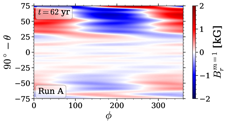
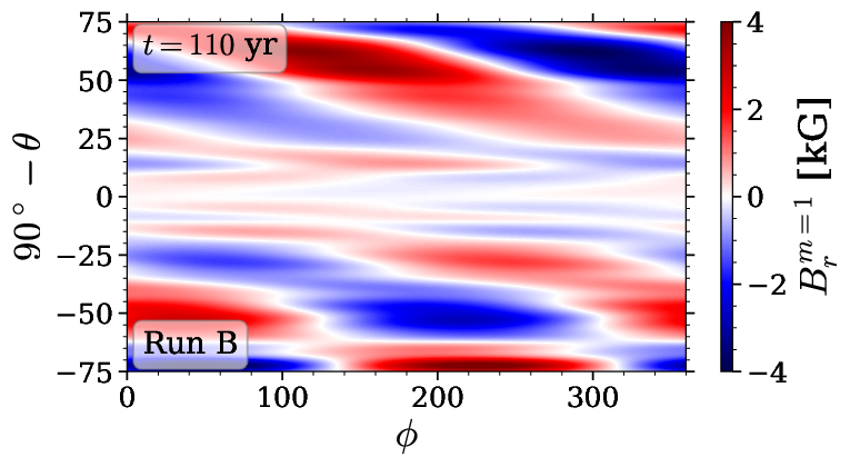
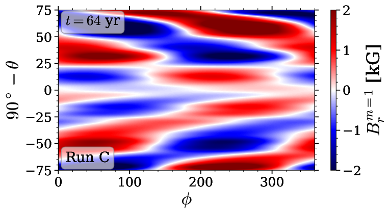
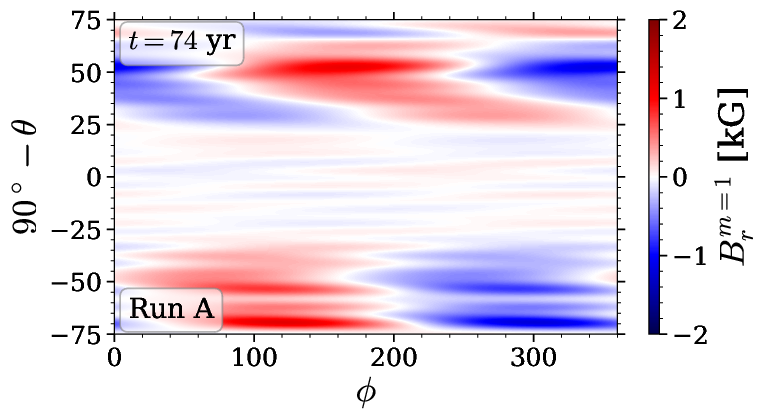
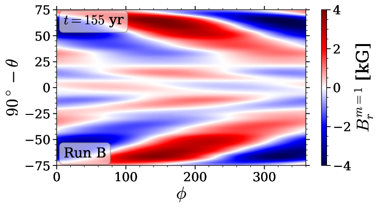
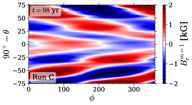
Figure 13: First nonaxisymmetric mode of the radial magnetic field ($B_{r}^{m=1}$) at $r=0.98R$ for each run.

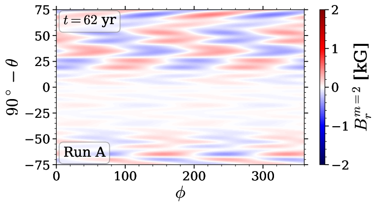
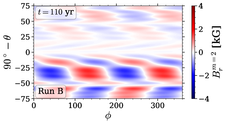
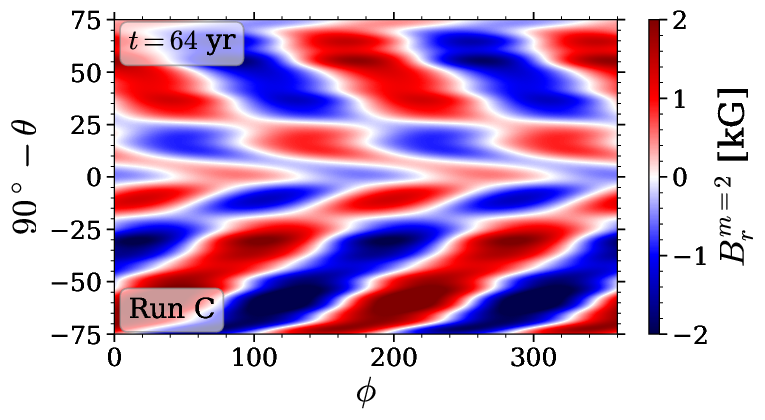
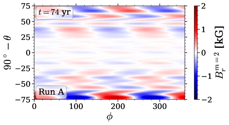
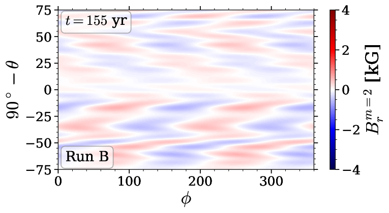
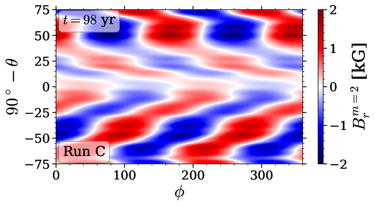
Figure 14: Second nonaxisymmetric mode of the radial magnetic field ($B_{r}^{m=2}$) at $r=0.98R$ for each run.

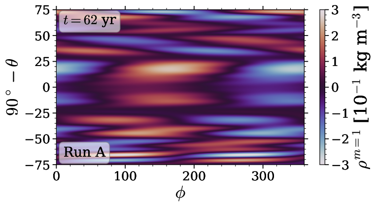
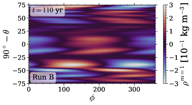
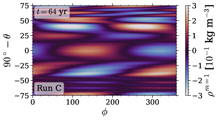
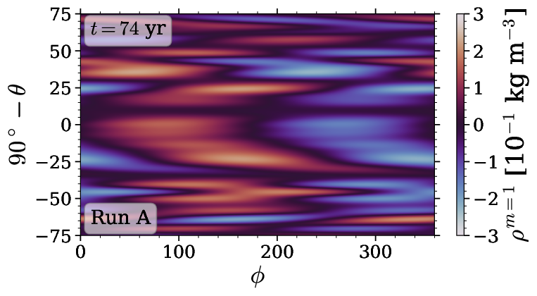
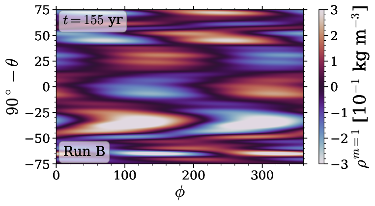
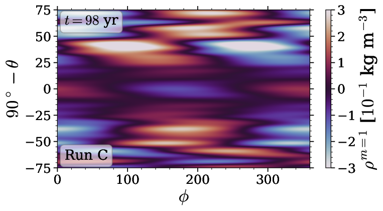
Figure 15: First nonaxisymmetric mode of density at $r=0.98R$ for each Run.

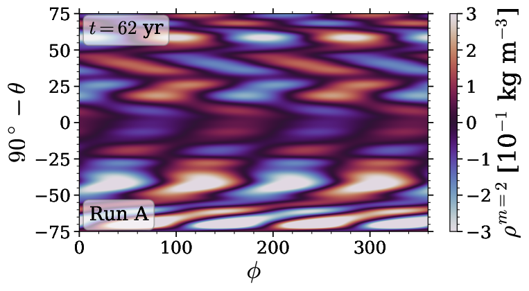
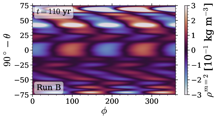
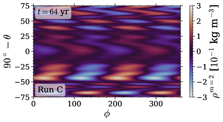
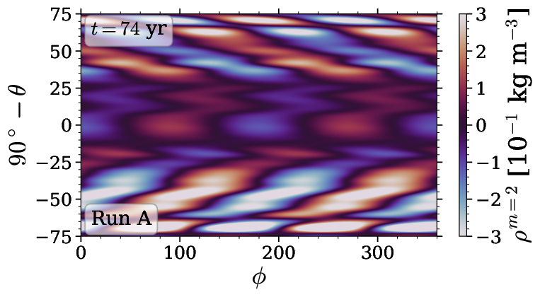
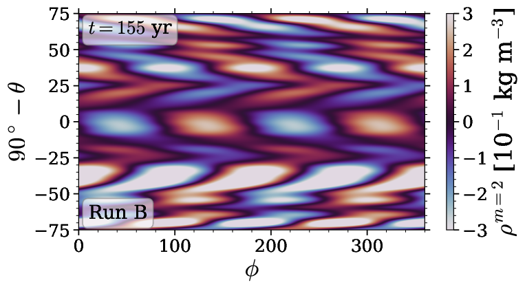
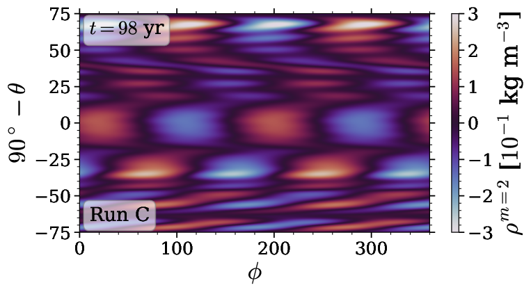
Figure 16: Second nonaxisymmetric mode of density at $r=0.98R$ for each Run.

To investigate the proposed connection between the nonaxisymmetric component of the magnetic field and the fluid density, we perform the same decomposition as in Viviani et al. (2018) for the radial magnetic field and density field at various radial depths (see Figures 13, 14, 15, and 16 for snapshots of the first and second nonaxisymmetric modes near the surface of the three runs.) A function $f=f(\theta,\phi)$ can be written as

$$f(\theta,\phi)=\sum_{l=0}^{l_{\rm max}}\sum_{m=-l}^{l}\tilde{f}_{\,l}^{\,m}(\theta,\phi)Y_{l}^{m}(\theta,\phi),$$ (7)

where

$$\tilde{f}_{\,l}^{\,m}=\int_{0}^{2\pi}\int_{\theta_{0}}^{\pi-\theta_{0}}f(\theta,\phi)\,Y_{l}^{m*}\sin{\theta}\,d\theta\,d\phi.$$ (8)

For the radial magnetic field $B_{r}(\theta,\phi)$, we impose the condition (see Krause & Rädler, 1980)

$$B_{r,l}^{-m}=(-1)^{m}B_{r,l}^{m*},$$ (9)

and because the same property applies to the spherical harmonics $Y_{l}^{m}$, we have

$$B_{r}(\theta,\phi)=\sum_{l=1}^{l_{\rm max}}B_{l,r}^{0}Y_{l}^{0}+2\,{\rm Re}\left(\sum_{l=1}^{l_{\rm max}}\sum_{m=1}^{l}B_{l,r}^{m}Y_{l}^{r}\right).$$ (10)

The term containing $l=0$ has been dropped because it violates solenoidality of the magnetic field.

2.3 Simulation parameters

Each run is characterized by the Taylor, Coriolis, fluid and magnetic Reynolds numbers, and fluid, SGS and magnetic Prandtl numbers. These are defined as

$${\rm Ta}=\!\left[\frac{2\Omega_{0}(0.3R)^{2}}{\nu}\right]^{2},\ {\rm Co}=\frac{2\Omega_{0}}{u_{\rm rms}k_{1}},$$ (11)

$${\rm Co}^{(\omega)}=\frac{2\Omega_{0}}{\omega_{\rm rms}},\ {\rm Re}=\frac{u_{\rm rms}}{\nu k_{1}},\ {\rm Re_{M}}=\frac{u_{\rm rms}}{\eta k_{1}},$$ (12)

$${\rm Pr}=\frac{\nu}{\chi_{m}},\ {\rm Pr_{M}}=\frac{\nu}{\eta},\ {\rm Pr_{\rm SGS}}=\frac{\nu}{\chi_{\rm SGS}^{\rm m}},$$ (13)

where $\nu$ is the viscosity, $u_{\rm rms}$ the root-mean-square velocity, ${\rm Co}^{(\omega)}$ is an alternative definition of the Coriolis number based on the rms vorticity, $k_{1}=2\pi/0.3R$ an estimate of the wavenumber of the largest convective eddies, $\eta$ the magnetic diffusivity, and $\chi_{\rm SGS}^{\rm m}$ is the SGS entropy diffusion at $r=0.85\leavevmode\nobreak\ R_{\odot}$.

3 Results

We present the results of three runs, labeled as A, B, and C, with rotation periods of 8.3, 1.2 days, and 0.8 days, corresponding to 3, 20, and 30 times the solar rotation rate. We keep all other sytem parameters fixed.

Table 1: Summary of simulation parameters.

Run	$\Omega/\Omega_{\odot}$	$P_{\rm rot}$ (days)	Ta	Co	Co(ω)	Ma	Re	ReM	Pr	PrM	PrSGS	$\Delta$t [yr]
A	3	8.3	$5.68\times 10^{7}$	2.8	1.28	$6.46\times 10^{-2}$	66.6	66.6	58	1.0	2.5	39
B	20	1.2	$2.52\times 10^{9}$	62.4	12.4	$3.29\times 10^{-2}$	20.3	20.3	58	1.0	2.5	138
C	30	0.8	$5.68\times 10^{9}$	139.1	22.4	$2.06\times 10^{-2}$	13.6	13.6	58	1.0	2.5	145

We summarize input and diagnostic quantities that characterize each simulation in Table 1.

3.1 Magnetic activity and quadrupole moment evolution

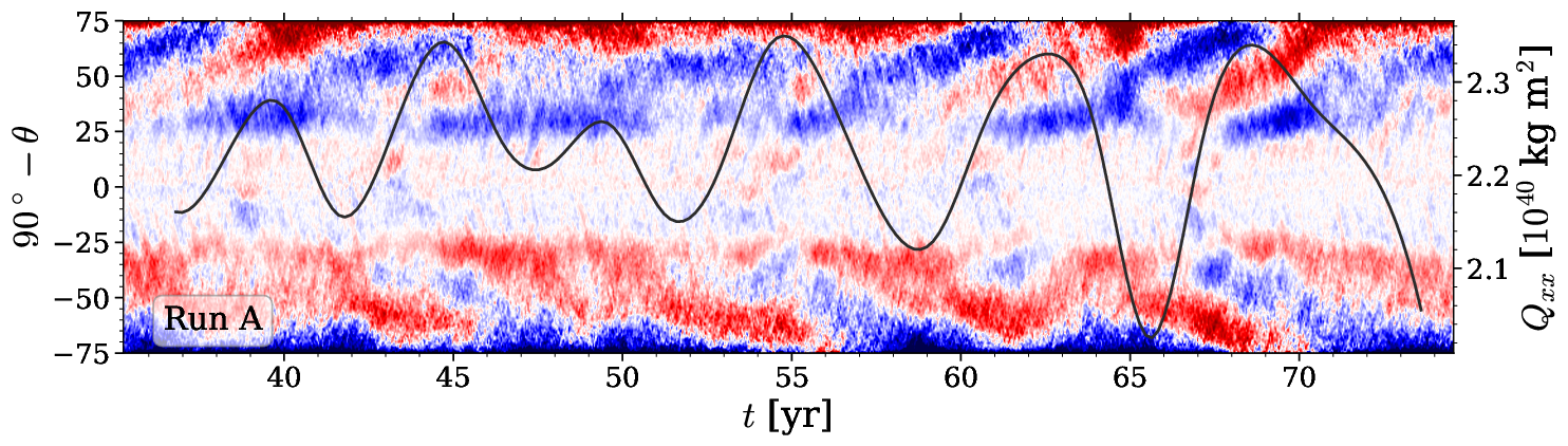
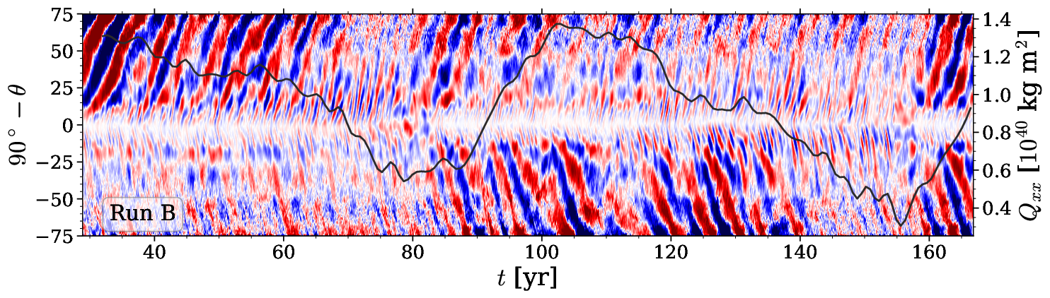
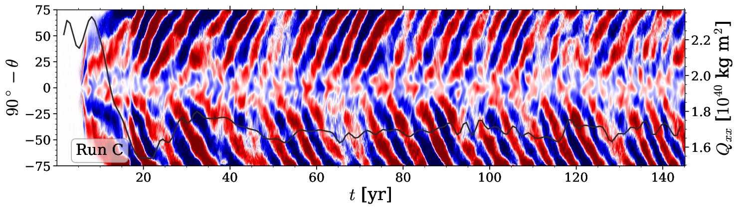
Figure 1: Azimuthally averaged radial magnetic field ($\overline{B}_{r}$) near the surface of the domain at $r=0.98R$ as a function of latitude and time for Run A (top, $P_{\rm rot}=8.3$ d), Run B (middle, $P_{\rm rot}=1.2$ d), and Run C (bottom, $P_{\rm rot}=0.8$ d). $Q_{xx}$ for each run is shown from the time periods where this diagnostic is available. The color scale of $\overline{B}_{r}$ in each panel has been clipped at $\pm 8$ kG.

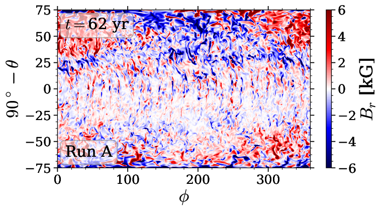
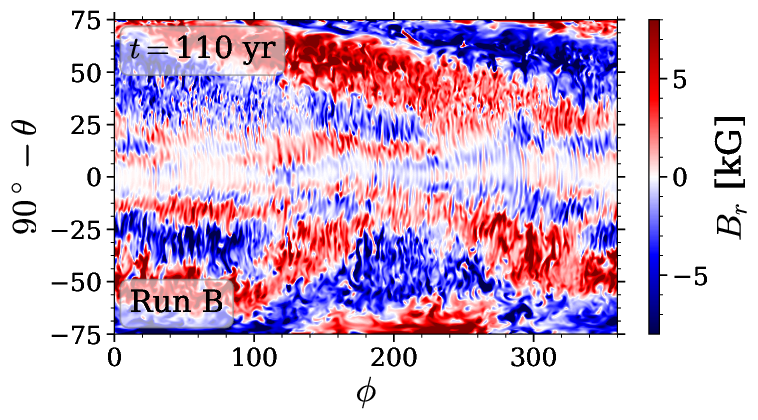
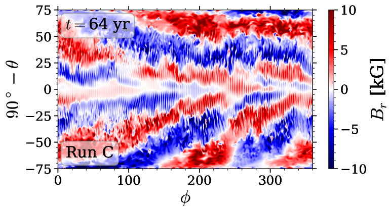
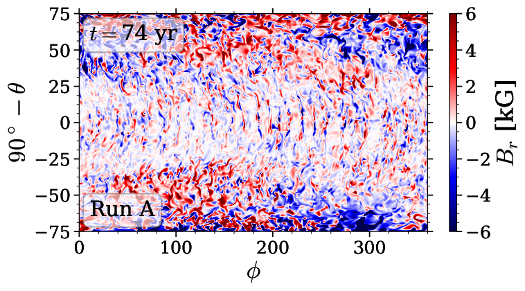
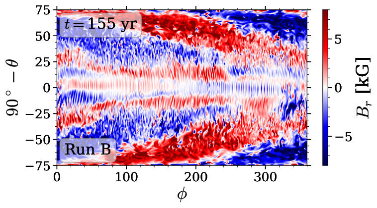
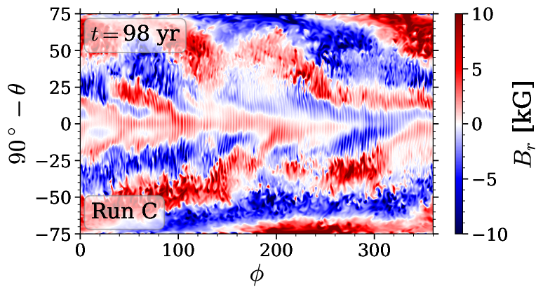
Figure 2: Instantaneous radial magnetic field at $r=0.98R$ for each run at two times. Top (bottom) row corresponds to a maxima (minima) of $Q_{xx}$.

We begin our analysis by comparing the time-dependent diagnostics of magnetic fields and the gravitational quadrupole moment. in Figure 1 we show the azimuthally averaged radial magnetic field ($\overline{B}_{r}$) near the surface of the stars at $r/R=0.98$ (color contours), along with the evolution of the $xx$ component of the gravitational quadrupole moment $Q$ (black lines). The latter is defined as

$$Q_{ij}=I_{ij}-\frac{1}{3}\delta_{ij}\,{\rm Tr}I,$$ (14)

where

$$I_{ij}=\int\rho({\bm{x}})x_{i}x_{j}{\rm d}V$$ (15)

is the $ij$ component of the inertia tensor expressed in Cartesian coordinates and $\rho({\bm{x}})$ is the density. All of the simulations show low-amplitude variations of $Q_{xx}$ on a timescale of roughly $0.2$ years. These are attributed to sound waves and have a purely hydrodynamic origin (Navarrete et al., 2020). Hence such signals are left out of the data in this study by working with low-cadence snapshots and interpolating the data with a cubic interpolator. In Run A, the variations of $Q_{xx}$ are small, on the order of $10^{39}...2\times 10^{39}$ kg m² and by visual inspection we estimate that they have a similar period (roughly 6-8 years) as the axisymmetric part of the magnetic field. Run B shows a larger amplitude long-term variation of $Q_{xx}$ that repeats at least once in the data. Roughly half of the data for Run B, up to about 80 years, was presented in Navarrete et al. (2020). The steady decrease of $Q_{xx}$ between $t\approx 30$ to $t\approx 85$ years was interpreted as a transient due to insufficient thermodynamic and magnetic saturation. However, with the longer time series we see that the quadrupole moment is modulated on a timescale of about 80 years. It also appears that $Q_{xx}$ is roughly correlated to $\overline{B}_{r}$: low values of the quadrupole moment approximately coincide with times when $\overline{B}_{r}$ is weak on both hemispheres ($t=70\ldots 85$ and $t=140\ldots 160$ years, respectively). The cycle is perhaps starting again at $t=160$ as the magnetic activity appears to be resuming with a corresponding change in $Q_{xx}$. The largest variation of $Q_{xx}$ occurs between $t=100...155$ years, with an amplitude of $10^{40}$ kg m². It corresponds to the largest variation of $Q_{xx}$ of the three runs. Overall, the gravitational quadrupole moment appears to follow the radial magnetic field strength near the surface of the star independently of the hemispheric asymmetry. In contrast to the other two runs, diagnostics for $Q_{xx}$ in Run C are available starting at $t=0$ yr. The quadrupole moment in this run remains more or less constant and only starts to decrease after the magnetic field approaches the saturated regime at $t\approx 10$ yr. The magnetic field back-reacts and re-adjusts the thermodynamic quantities, such as density, after which $Q_{xx}$ settles to a state with smaller variations around a mean value of $1.70\times 10^{40}$ kg m². These variations are about half of those in Run A. As seen in Fig. 1, the axisymmetric part of $B_{r}$ is similar in Runs A and C, but clearly different in Run B. In the first two, $\overline{B}_{r}$ migrates toward higher latitudes in a regular fashion and in the latter the dynamo is more hemispheric such that activity alternates between both hemispheres seemingly every 50 to 60 years. Overall, cycles of $Q_{xx}$ in Runs A and C follow more closely the polarity reversals of the magnetic field. There are also such cycles in Run B. However, they are hidden by the longer cycle that follows the migration of the hemispheric component of the magnetic field.

Table 2: Summary of some quantities of interest corresponding to data shown in Fig. 1.

Run	$Q_{xx}^{\rm{max}}$	$Q_{xx}^{{\rm min}}$	$\overline{B}_{r}^{\rm max}$	$\overline{B}_{r}^{\rm min}$	$E_{\rm mag,total}^{\rm max}$	$E_{\rm mag,total}^{\rm min}$
A	2.25	1.94	8.65	-9.70	2.98	1.26
B	1.38	0.315	24.7	-19.7	3.98	2.28
C	1.80	1.54	16.8	-13.8	2.32	1.30

In Fig. 2 we show instantaneous snapshots of the radial magnetic field near the surface of the three runs at the times of interest, that is, maxima (minima) of $Q_{xx}$ at top (bottom) row. These correspond to $t=62,74$ yr for Run A, $t=110,155$ yr for Run B, $t=64,98$ yr for Run C. In Run A, a predominantly $m=1$ large-scale mode is seen at high latitudes but this is subdominant in comparison to the axisymmetric ($m=0$) component (see Appendix B). In Run B there is a dominant $m=1$ mode on the northern hemisphere, while a predominantly $m=2$ mode dominates on the southern hemisphere at the maximum. At the minimum of $Q_{xx}$ (middle panel in the lower row), $B_{r}$ is symmetric with respect to the equator with a dominating $m=1$ mode on both hemispheres. These large-scale structures cover the entire hemispheres from the equator to the latitudinal boundaries. This is qualitatively similar to Run H of Viviani et al. (2018) and Run C of Cole et al. (2014). As suggested by Fig. 1, a similar pattern repeats for Run B at $t\approx 36$ yr and $t\approx 75$ yr but in opposite hemispheres. Run C is similar to Run B in the sense that the large-scale nonaxisymmetric structures are promiment over a large region, but the $m=1$ and $m=2$ modes appear to be similar in strength. These modes appear to alternate between the hemispheres but the variations in the gravitational quadrupole moment are weak in this case in comparison to Run B. However, the low-order nonaxisymmetric fields in Run C are of the same order of magnitude as the $m=0$ mode whereas in Run B the $m=1$ mode is clearly stronger than the axisymmetric fields. A possible explanation of the smaller cycles of $Q_{xx}$ found in Run C can be attributed to the dynamo solution. Slow rotators tend to produce dominant $m=0$ modes. Faster rotators typically show a predominant $m=1$ mode although sometimes the $m=0$ component can become dominant again at very high rotation rates if the convection is only weakly supercritical (Viviani et al., 2018). It is plausible that this is happening in our Run C. These results suggest that a dominant nonaxisymmetric magnetic field with hemispheric asymmetry is associated with the strongest variations of $Q$.

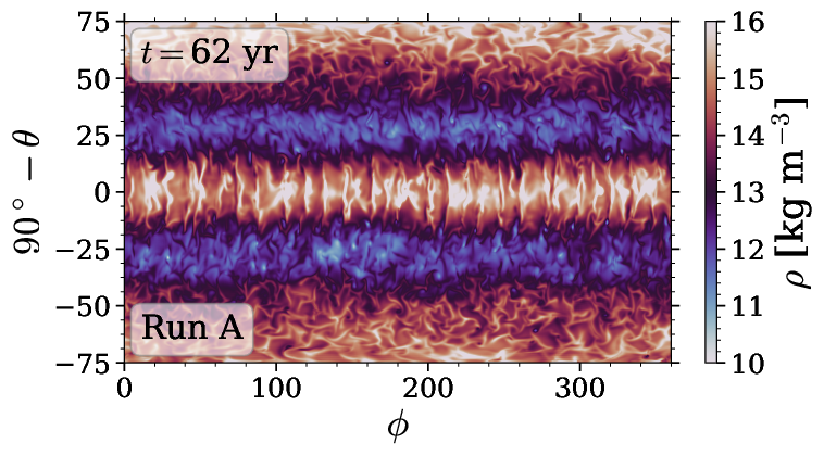
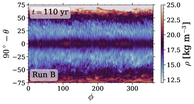
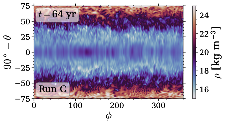
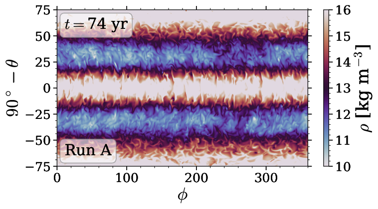
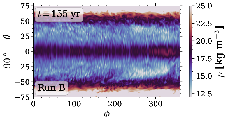
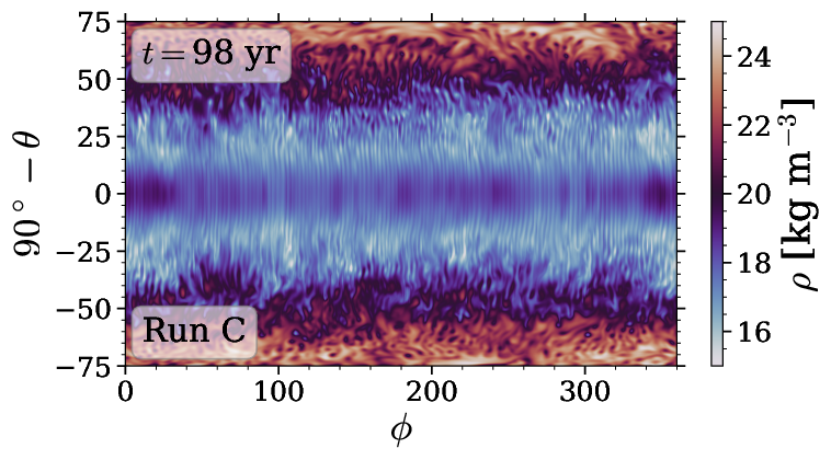
Figure 3: Instantaneous snapshots of density at $r=0.98R$ for each run.

3.2 Density variations and structural changes due to magnetic fields

The variations of the gravitational quadrupole moment are related to changes in the mass distribution within the star as can be seen from Eqs.(14) and (15). Snapshots of the density from all three runs near the surface of the star are shown in Fig. 3. As before, the shown times correspond to maxima (top row) and minima (bottom row) of $Q_{xx}$. Snapshots of the $m=1$ and $m=2$ modes of density are show in the Appendix B.

In Run A there is an overall change in density between the two times. At $t=62$ yr (top panel), when the gravitational quadrupole moment is larger, there are no noticeable large-scale nonaxisymmetric features, whereas when $Q_{xx}$ is at a minimum ($t=74$ yr), weak nonaxisymmetric features appear. This can be seen from the two blue stripes around $\theta=\pm 30^{\circ}$ where the overall density decreases with patches of increased (decreased) density around $\phi=270^{\circ}$ ($\phi=60^{\circ}$). Closer to the poles and near the equator the average density increases but no clear nonaxisymmetric features are present. In Run B we identify a few characteristics. First, when the quadrupole moment is larger at $t=110$ yr, there is a clear asymmetry with respect to the equator, such that the density is larger close to the north pole. As $Q_{xx}$ decreases, the asymmetry disappears, and nonaxisymmetric structures become visible at $230^{\circ}<\phi<340^{\circ}$ and $\theta=\pm 40^{\circ}$. As the magnetic field changes its configuration from one that is dominated by an $m=1$ mode only at the northern hemisphere to predominantly $m=1$ on both hemispheres (see Fig. 2), the density field reacts and also changes to a nonaxisymmetric configuration with a corresponding change in the gravitational quadrupole moment. In contrast, large-scale density variations in Run C between the two times are clearly weaker. The density field at the surface remains symmetric with respect to the equator as well as in the azimuthal direction.

To investigate the importance of equatorial asymmetry on the gravitational quadrupole moment, we define the equatorially asymmetric part of density as

$$\rho_{\rm asym}(r,\theta,\phi)=\frac{\rho(r,\theta,\phi)-\rho(r,-\theta,\phi)}{2}$$ (16)

and compute the root mean square according to

$$\rho_{\rm s,rms}=\left(\langle\rho_{\rm asym}^{2}\rangle_{\theta\phi}\right)^{1/2}.$$ (17)

The time evolution of $\rho_{\rm s,rms}$, together with $Q_{xx}$, is shown in the top row of Fig. 4. In Run A (left panel) there is an anticorrelation between the two. However, in the case of Run B (middle panel) there is a positive correlation between the two but with an apparent time delay. The rms value of $\rho_{\rm s,rms}$ lags behind $Q_{xx}$ by roughly $10$ yr for example near the extrema between $80$ and $100$ yr. In Run C both the variations of the density and $Q_{xx}$ are weak. It is also less clear whether a correlation between the two exists.

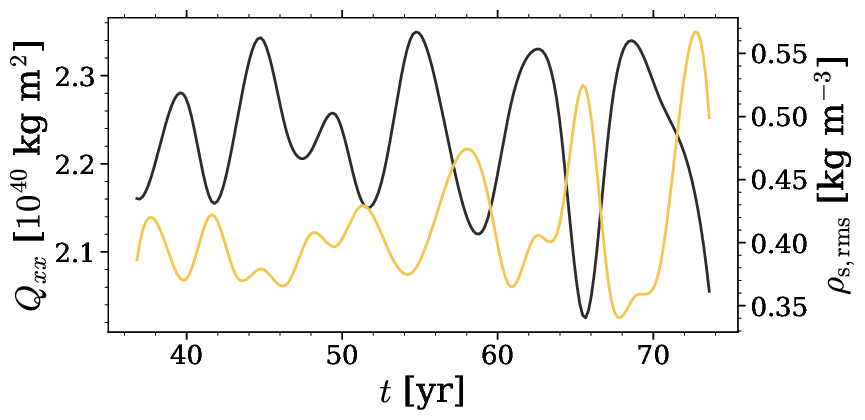
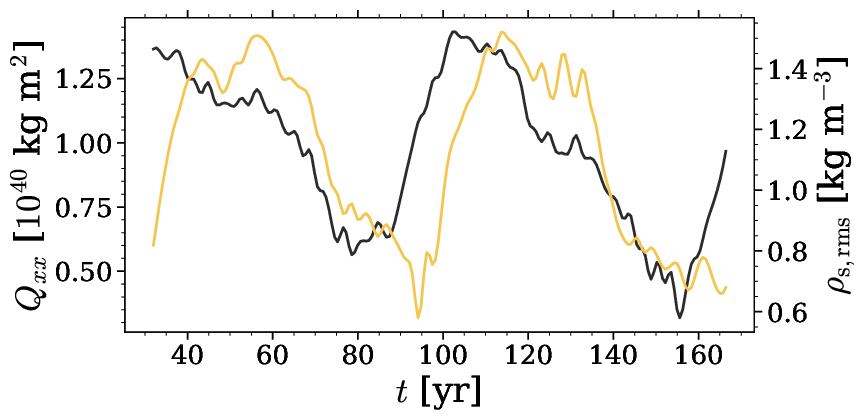
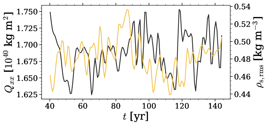
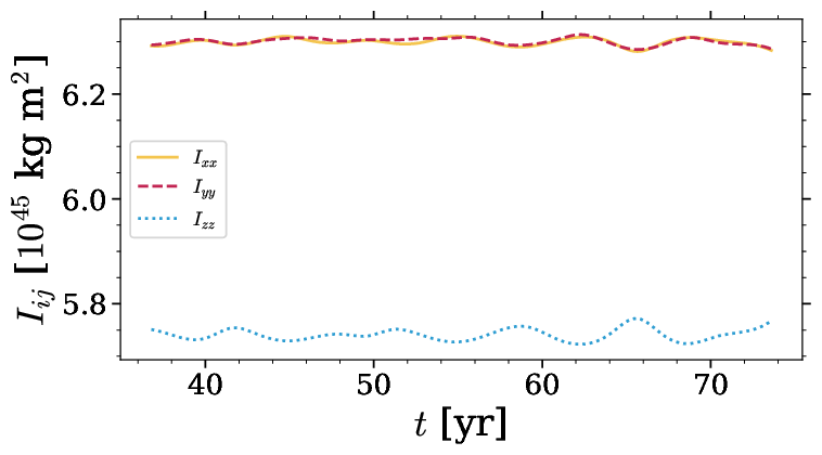
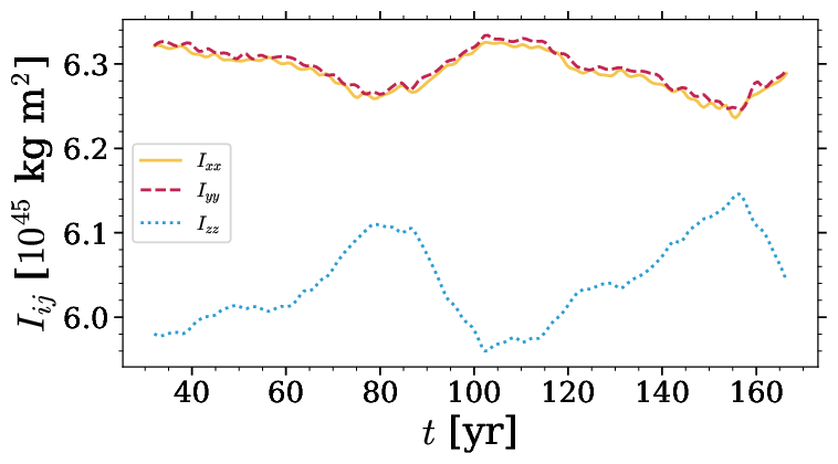
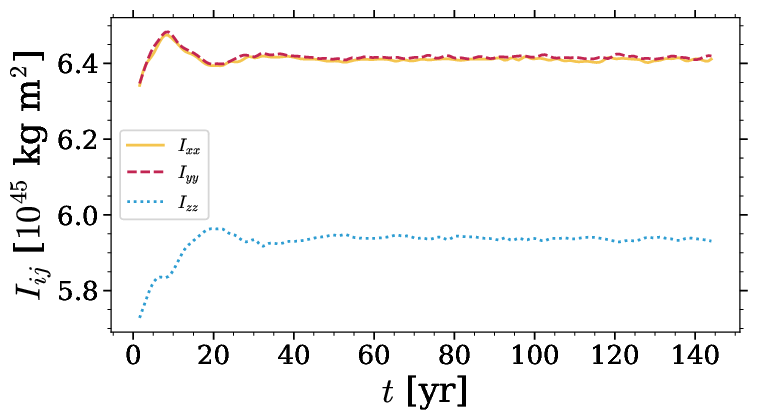
Figure 4: Top row: $Q_{xx}$ (black) and rms value of the equatorically asymmetric part of density $\rho_{\rm s,rms}$ (yellow) according to Eq. (17) as functions of time. Bottom row: time evolution of the diagonal components of the inertia tensor. First, second, and third columns correspond respectively to runs A, B, and C.

The variations of $\rho_{\rm s,rms}$ are between 6 to 10 times larger in Run B than in Runs A and C, indicating that the former is in a different dynamo regime where the magnetic field is more strongly coupled to the density field leading to stronger quadrupole moment variations.

The differences in density with respect to the equator should translate in variations of the moment of inertia aligned with the rotational axis of the star, namely, $I_{zz}$. The lower row of Figure 4 shows the evolution of the three components of the inertia tensor that contribute to $Q_{xx}$, which is computed from

$$Q_{xx}=I_{xx}-\frac{1}{3}\left(I_{xx}+I_{yy}+I_{zz}\right).$$ (18)

The vertical component $I_{zz}$ is always smaller than the two other components. In Runs A and C all components of $I_{ij}$ have comparable variations, whereas in Run B (middle panel) the variations of $I_{zz}$ are significantly larger. This coincides with larger variations of $\rho^{m=1,2}$ in this run. In Run B a maximum of $Q_{xx}$ coincides with a minimum of $I_{zz}$. This corresponds to the star rotating slightly faster at maxima (minima) of $Q_{xx}$ ($I_{zz}$).

To see such differences, we compute the azimuthally averaged rotation profiles

$$\overline{\Omega}(r,\theta)=\Omega_{0}+\frac{\overline{u}_{\phi}(r,\theta)}{r\sin\theta}$$ (19)

for all runs, average them over time, and show the deviations from such averages during the two times of interest in Fig. 5. There are minor differences in the rotation profiles of Runs A and B between maxima and minima of $Q_{xx}$, while almost no differences are observed in Run C. Runs A and B have a larger difference between angular velocities of polar and equatorial regions at a minima of $Q_{xx}$ (lower panels), but an accelerated northern pole is seen in the top panel of Run B. A large difference in differential rotation implies that the star would deform and adopt an ellipsoidal shape as a consequence of the centrifugal force, adding a further contribution to the quadrupole moment. However, as we have fixed boundary conditions, we cannot model such a reaction. All of our runs show a solar-like rotation profile with equatorial regions rotating faster than the poles as a consequence of Coriolis numbers above the transition region from antisolar to solar-like differential rotation. This transition occurs around $\rm{Co}\gtrsim 1$ (see e.g., Gastine et al., 2014; Käpylä et al., 2014) whereas the rotation profile approaches solid body rotation for rapid rotation (e.g., Viviani et al., 2018; Käpylä, 2021).

Table 3: Correlation coefficients between the time series of the quadrupole moment and magnetic energy, mean surface density and quadrupole moment, and mean surface density and magnetic energy

. Run $Q_{xx}|E_{\rm mag}^{m=0}$ $Q_{xx}|E_{\rm mag}^{m=1}$ $Q_{xx}|E_{\rm mag}^{m=2}$ $\overline{\rho}_{\rm surf}|Q_{xx}$ $\overline{\rho}_{\rm surf}|E_{\rm mag}^{m=0}$ $\overline{\rho}_{\rm surf}|E_{\rm mag}^{m=1}$ $\overline{\rho}_{\rm surf}|E_{\rm mag}^{m=2}$ A -0.41 0.54 0.13 -0.67 0.20 -0.18 -0.07 B 0.38 -0.64 0.66 -0.94 -0.40 -0.53 -0.57 C 0.26 0.22 -0.34 -0.40 0.25 0.11 -0.11

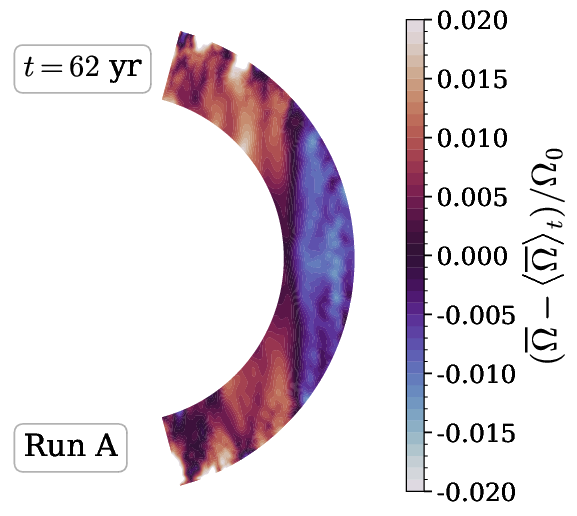
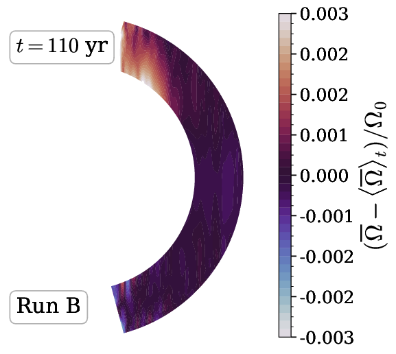
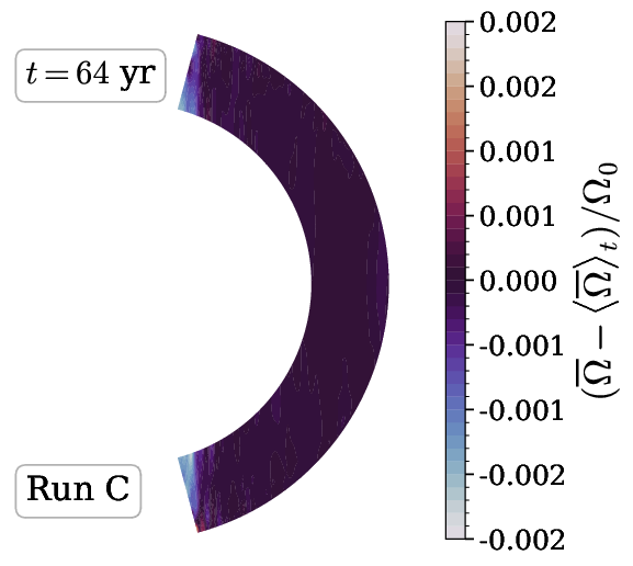
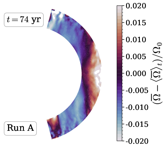
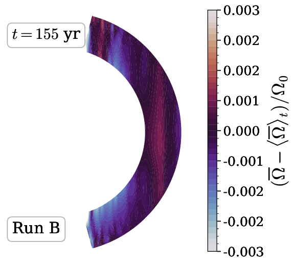
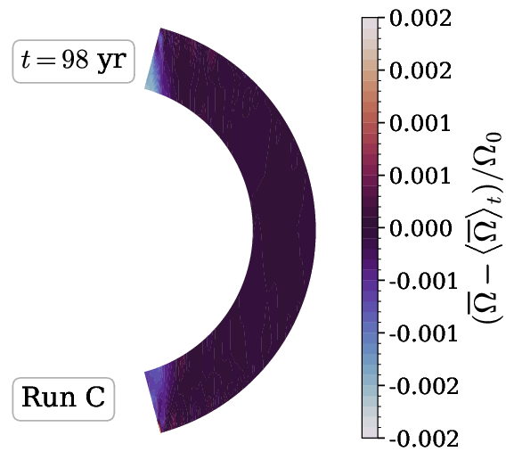
Figure 5: Deviations from the time-averaged mean angular velocity $(\overline{\Omega}-\langle\overline{\Omega}\rangle_{t})$ normalized by the angular velocity of the frame of reference $(\Omega_{0})$ for each run from the times indicated in the legends.

The energies of the axisymmetric and first two nonaxisymmetric modes of $B_{r}$ are shown in the lower row of Fig. 6 and a scatter plot between $B_{r}^{m=i}$ and $Q_{xx}$ is shown in the upper row. In Run A (first column) the axisymmetric $m=0$ is dominant, which seems to be anticorrelated with $Q_{xx}$. There are short episodes where the $m=0$ and $m=1$ modes have comparable energies. The latter is correlated to $Q_{xx}$. In Run A, the $m=2$ mode is always subdominant. From the scatter plot we see that no noticeable increase in magnetic energy is needed to reach a larger quadrupole moment. The situation in Run B is different as there is a persistent $m=1$ mode that dominates throughout the simulation with minor fluctuations in its energy. The axisymmetric mode seems to be correlated to $Q_{xx}$. This is because, as explained in the previous section, it produces equatorially asymmetric density fluctuations that modulate the moment of inertia aligned with the rotation axis of the star. The second nonaxisymmetric mode ($m=2$) is as strong as the axisymmetric mode and also correlates with $Q_{xx}$. Larger quadrupole moment values are related to higher energies in the $m=0$ and $m=2$ modes. In Run C all modes have similar energy levels, with $m=0$ being slightly stronger than the other two. The scatter plot reveals that there is no relation between the magnetic energy and the quadrupole moment.

To quantify the relation between magnetic field modes and quadrupole moment, we perform a correlation analysis. We use the Pearson correlation coefficient to study the linear correlation between the density and magnetic fields. The coefficient between a paired data $(x,y)$ of $n$ pairs is defined as

$$x|y=\frac{\sum_{i=1}^{n}(x_{i}-\bar{x})(y_{i}-\bar{y})}{\sqrt{\sum_{i=1}^{n}(x_{i}-\bar{x})^{2}}\sqrt{\sum_{i=1}^{n}(y_{i}-\bar{y})^{2}}},$$ (20)

where $\bar{x}$ and $\bar{y}$ are the sample mean and $-1\leq x|y\leq 1$. A value of $x|y=1$ ($x|y=-1$) implies perfect (anti-)correlation.

The correlations between the gravitational quadrupole moment and magnetic energy are calculated using the data presented in Fig. 6 and in this case the barred quantities in Eq. 20 represent time averages of $Q_{xx}$ and $E_{\rm mag}$, whereas $x_{i}$ and $y_{i}$ are the time-dependent quantities of $Q_{xx}$ (calculated over the whole volume) and $E_{\rm mag}$ (calculated over the surface layer). This is shown in the second, third, and fourth columns of Table 3. In general, we find correlations higher than 0.5 for the $m=1$ mode in Run A and for the $m=1$ and $m=2$ modes in B.

Next, we compute the correlation coefficients between the mean surface density $\overline{\rho}_{\rm surf}$ and quadrupole moment, and $\overline{\rho}_{\rm surf}$ and the magnetic energies. These are shown in the last four columns of Table 3. In each run we find that the values of $\overline{\rho}_{\rm surf}|Q_{xx}$ are relatively large. This is due to the direct relation between the density distribution and $Q_{xx}$. The outer regions of the stars are particularly important due to the $x^{2}$ dependence of the inertia tensor. As noted earlier, the dynamo solution in Run B alternates between the two hemispheres and so does the density field. As $\overline{\rho}_{\rm surf}$ increases, so does $I_{zz}$ and thus $Q_{xx}$ decreases (see Eq. 18). Overall, we see the clearest correlations in Run B.

The magnetic energy increases with the rotation rate as expected, but this does not suffice to explain the variations in the gravitational quadrupole moment. Overall, Run B has the largest magnetic energy and Run A and C have comparable energies (see Table 2). However, Run C has smaller fluctuations in $Q_{xx}$ which can be attributed to the fact that the variations of the magnetic field do not result in significant density perturbations relevant for the quadrupole moment.

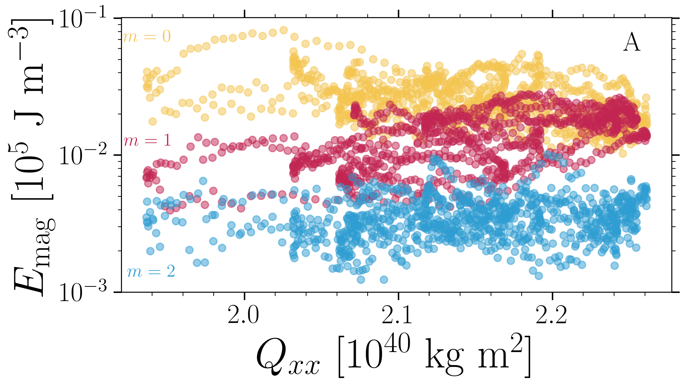
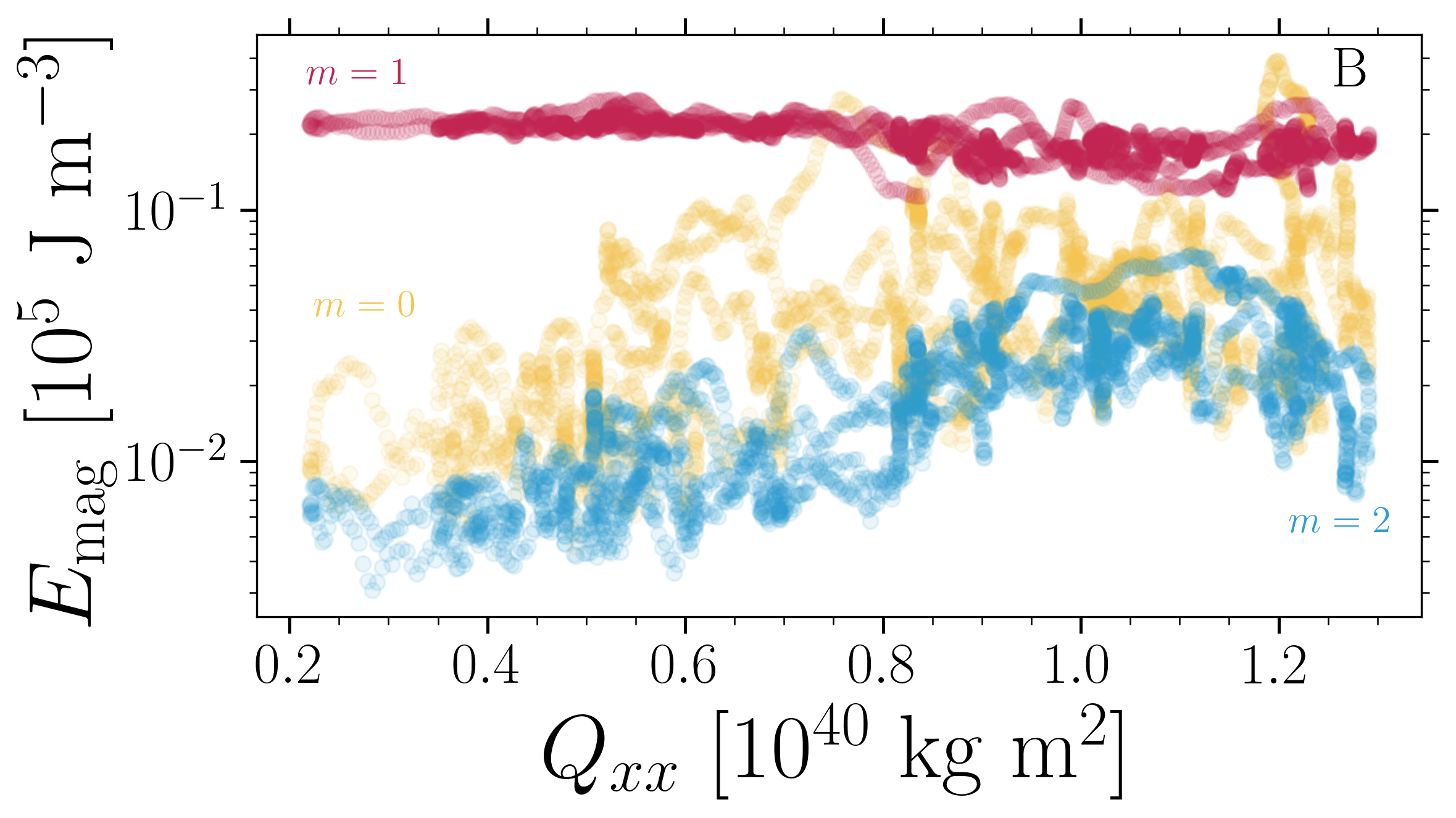
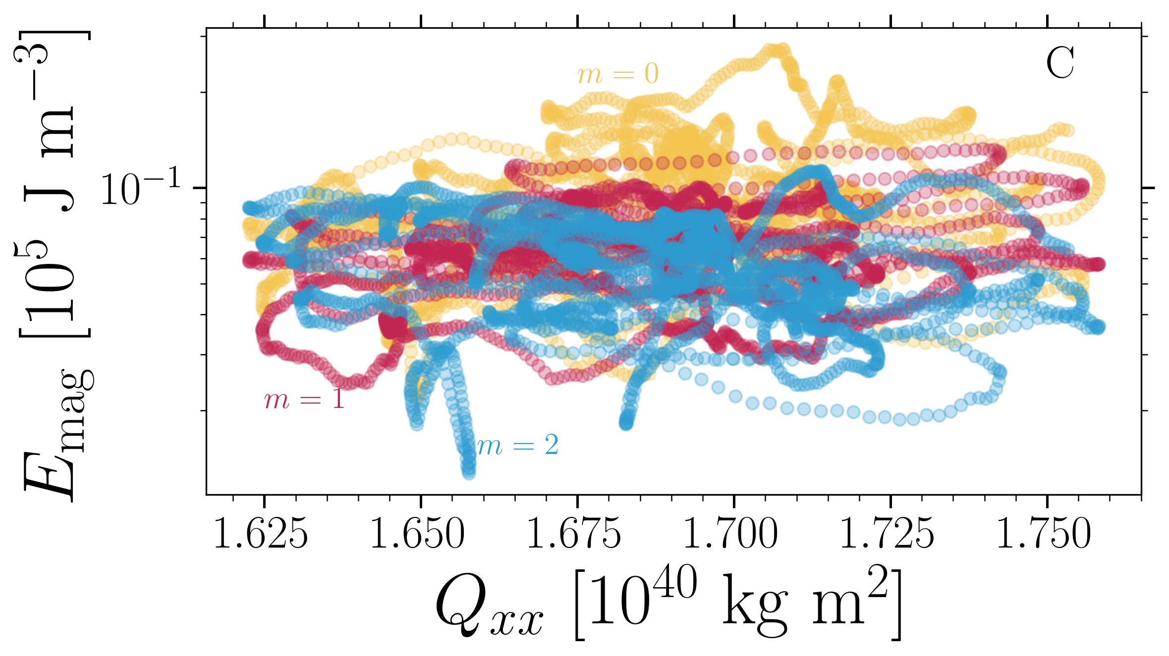
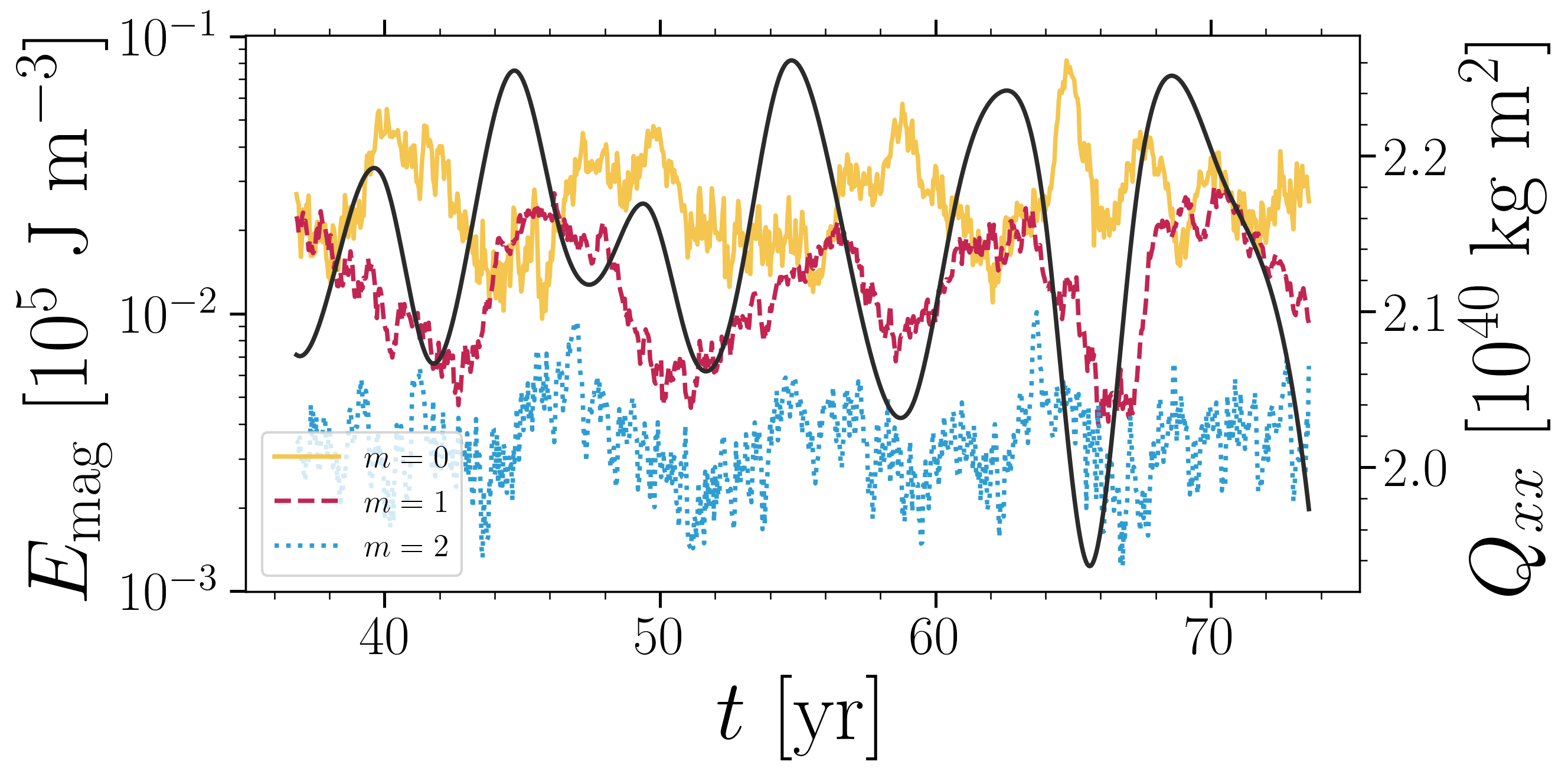
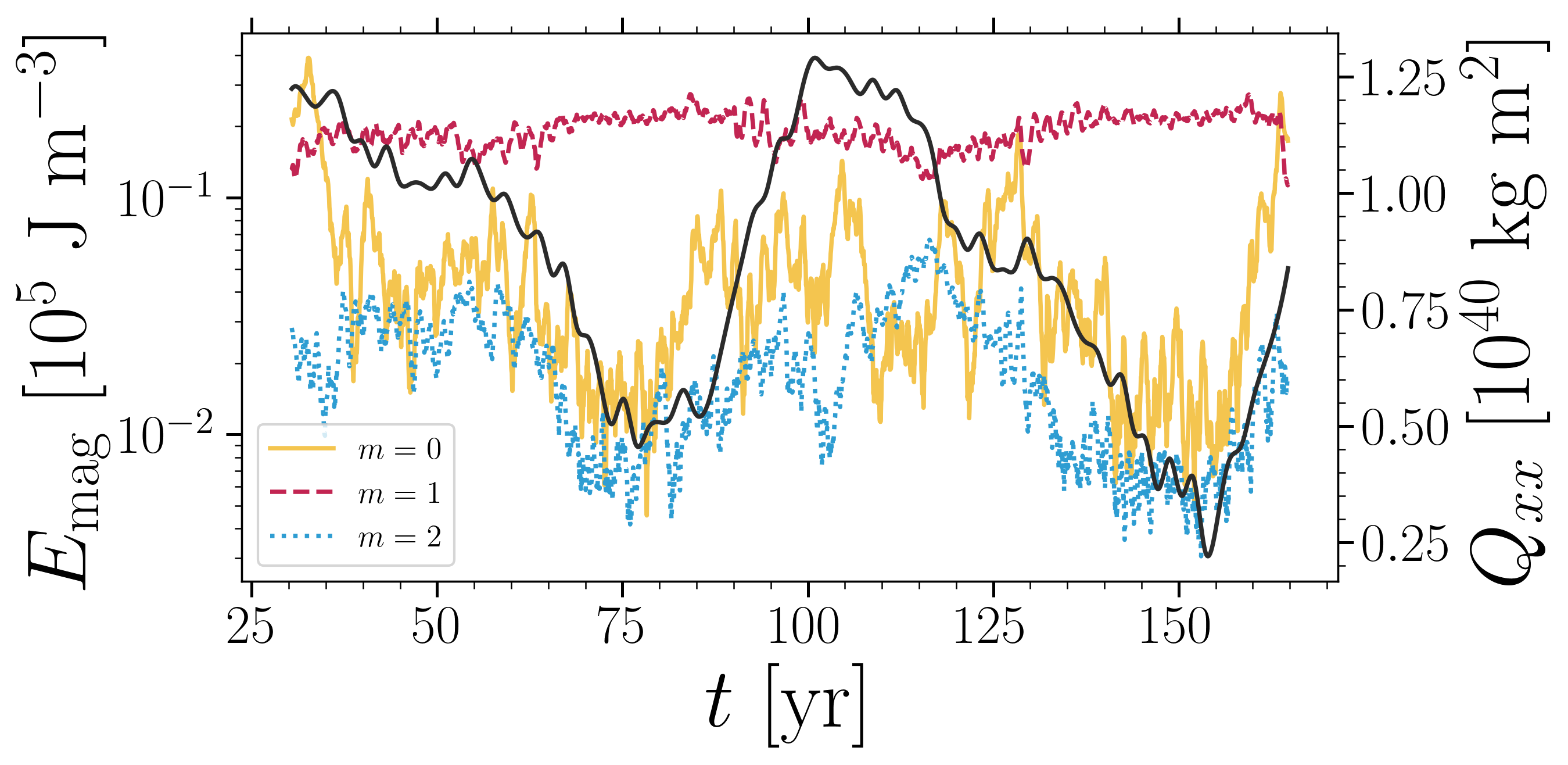
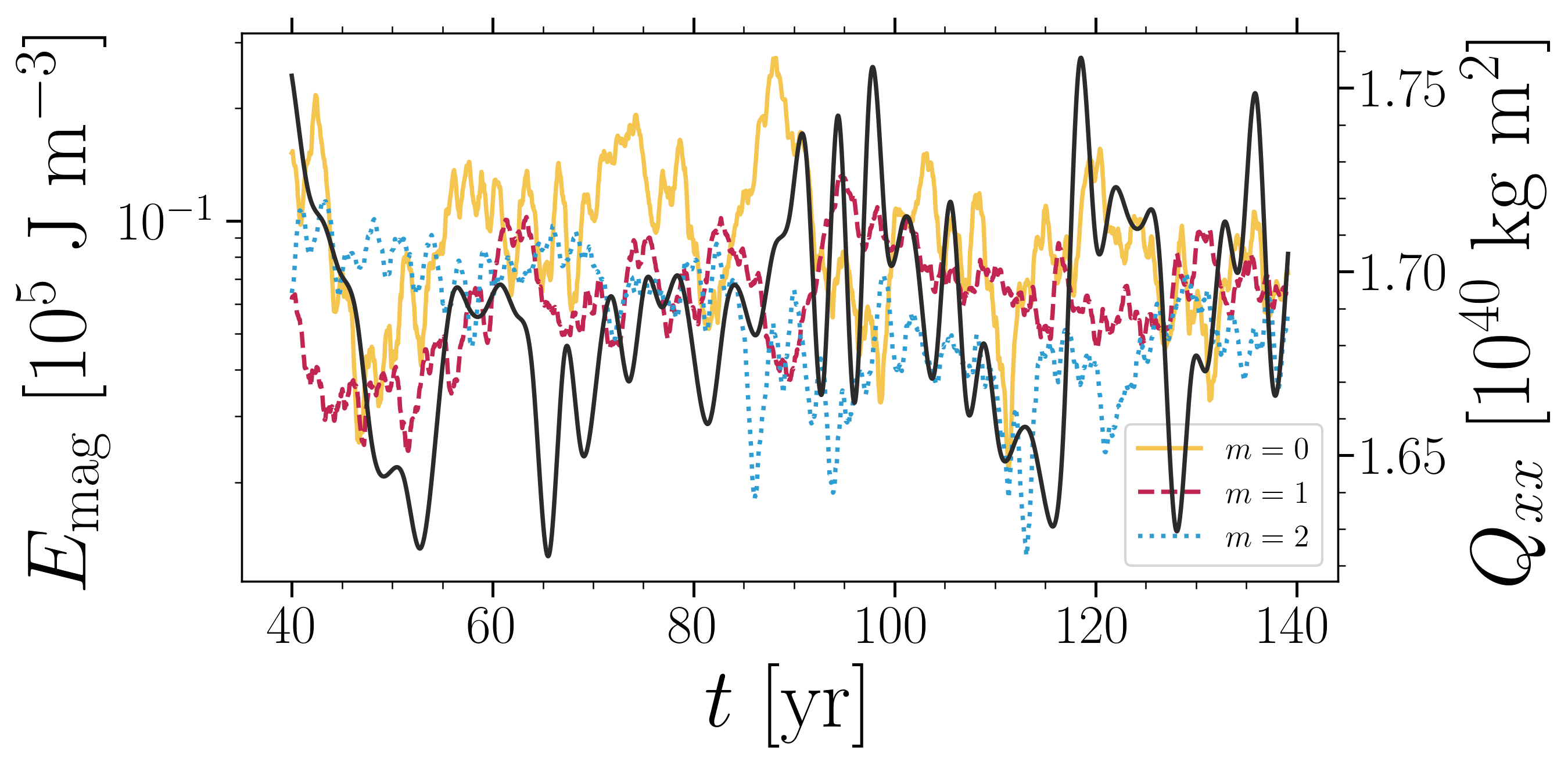
Figure 6: Quadrupole moment, density, and moments of inertia. Top row: scatter plot of the magnetic field energy and the quadrupole moment. Bottom row: Time evolution of the gravitational quadrupole moment (black line) together with the magnetic energy contained in the axisymmetric mode ($m=0$, yellow), as well as the first ($m=1$, red) and second ($m=2$, blue) non -axisymmetric modes. Run A, Run B, and Run C are shown in the left, middle, and right columns respectively.

3.3 Azimuthal dynamo waves

Azimuthal dynamo waves (ADWs) are magnetic structures that migrate in the azimuthal direction. ADWs can be prograde or retrograde and their propagation is unaffected by the differential rotation of the star (see e.g. Krause & Rädler, 1980; Cole et al., 2014; Viviani et al., 2018). The periods of ADWs are usually on the order of a few years for slow rotators and of tens of years for faster rotators (Viviani et al., 2018). This is comparable to the period of the quadrupole moment variations of the present study. We therefore briefly study ADWs. We take $m=1$ and $m=2$ modes of the radial magnetic field near the surface of each run at latitude $+60^{\circ}$ and show the evolution of the field in Fig. 7 and its phase in Fig. 8.

Run A has an $m=1$ ADW that migrates in the retrograde direction with a period of $\sim 8$ years in particular after around $t=60$ yr. Meanwhile, the $m=2$ ADW has a similar amplitude with no clear periodicity. In Run B there is a clear $m=1$ wave which migrates in the prograde direction. However, between 115 and 145 yr the migratory process is stalled for nearly thirty years. The ADW in Run B has a period of roughly $\sim 80...100$ years. There is an $m=2$ ADW but it is only noticeable during the first $\sim 40$ years of the simulation. In Run C there are two equally strong ADWs. Both migrate in a prograde way with the difference that the period of the $m=1$ wave is shorter than the one of $m=2$.

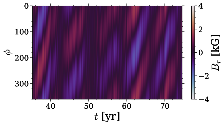
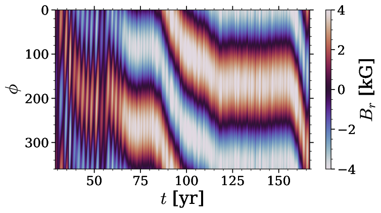
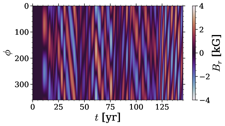
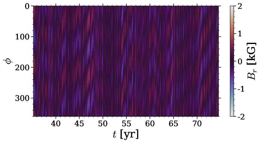
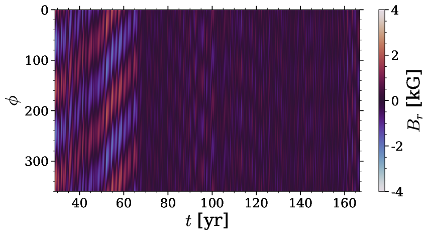
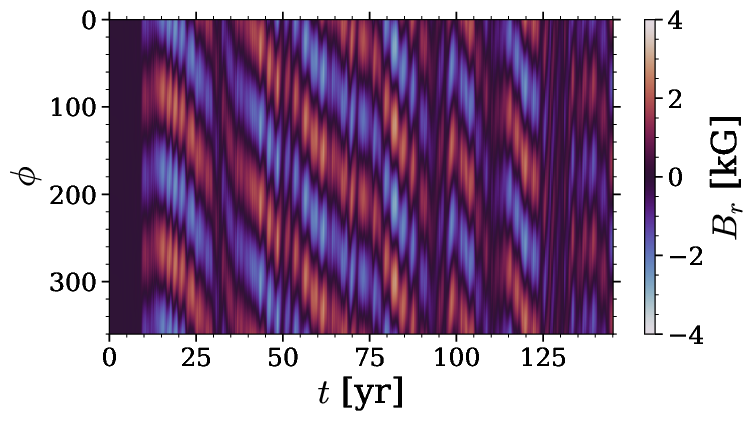
Figure 7: Migration of the $m=1$ (top row) and $m=2$ (bottom row) modes of the radial magnetic field at the surface along the longitudinal direction. for Run A (left), Run B (middle), and Run C (right).

The evolution of the phase of the $m=1$ mode correlates well with the evolution of the gravitational quadrupole moment in Runs A and B, whereas the second nonaxisymmetric mode is noisier and does not correlate with $Q_{xx}$. The phase of $B_{r}^{m=1}$ does not show any particular evolution in Run C, while for $m=2$ the phase is constantly decreasing which is uncorrelated with $Q_{xx}$. The cases of Runs A and B point to an underlying relation between a nonaxisymmetric dynamo mode and the gravitational quadrupole moment evolution.

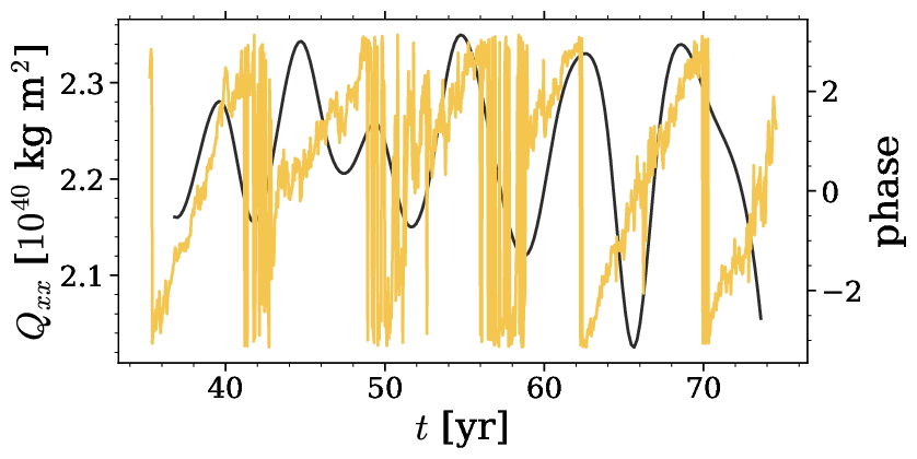
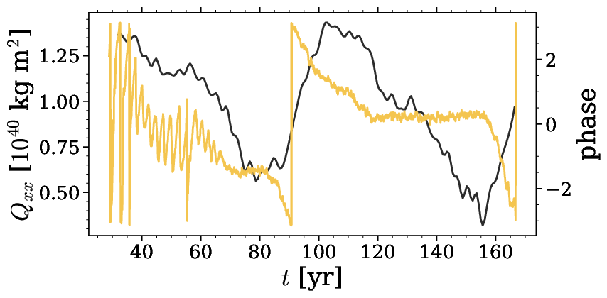
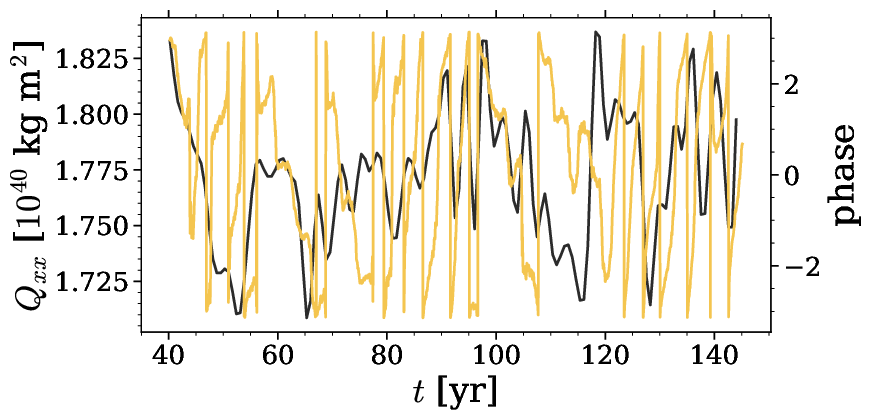
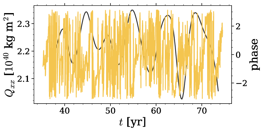
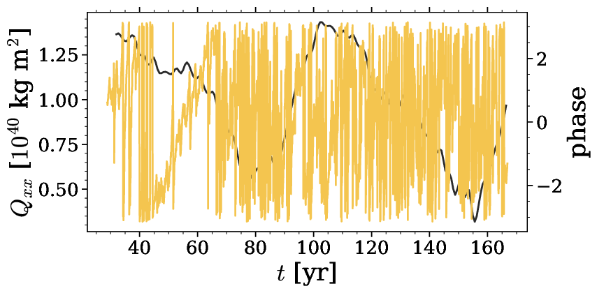
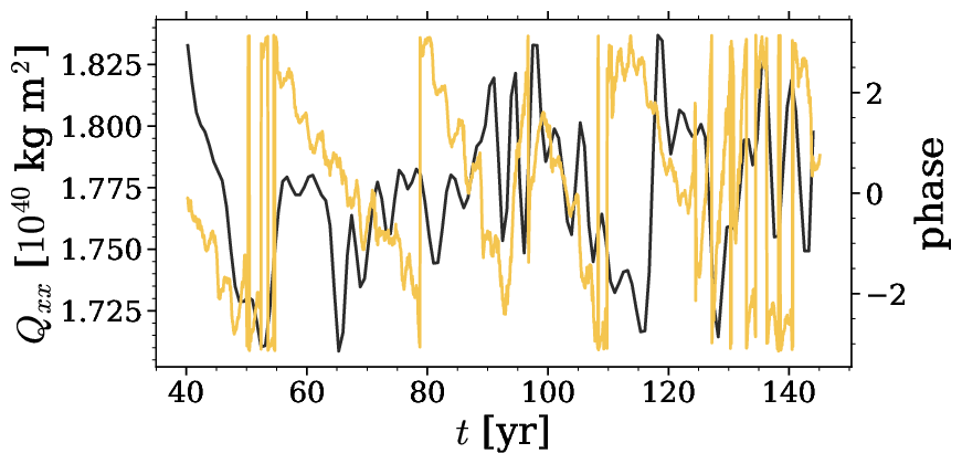
Figure 8: Time evolution of the phase of the $m=1$ (top row) and $m=2$ modes (bottom row) of radial magnetic field at $\phi=180^{\circ}$ for Run A (left panels), Run B (middle panels), and Run C (right panels) in yellow. The black line corresponds to $Q_{xx}$.

4 Discussion and implications

The Applegate mechanism (Applegate, 1992) is based on the redistribution of angular momentum throughout the star due to the centrifugal force. More recently, Lanza (2020) presented a new mechanism where the centrifugal force is no longer needed. In this work the quadrupole moment is constant in the frame of reference of the magnetically active star due to a time-invariant nonaxisymmetric magnetic field modeled by a single flux tube. The companion star experiences a time-varying nonaxisymmetric gravitational quadrupole moment due to the assumption that the active star is not tidally locked.

In our simulations we compute the gravitational quadrupole moment in the rotating frame of reference of the star. The simulations thus provide a test whether magnetic activity can significantly influence stellar structure. We stress that the physical process occurring here is not the classical Applegate mechanism which is based on the centrifugal force, and which is not included in our simulations. The results described in Sect. 3 show that the connection between magnetic fields and gravitational quadrupole moment is quite complex. It is due to the asymmetry of the magnetic field with respect to the equator rather than due to nonaxisymmetry, which is particularly noticeable in Run B. The three simulations we present differ only in the rotation rate of the star and yet they present different scenarios of quadrupole moment variations.

4.1 Behavior of the dynamo itself

Simulations of stellar magneto-convection have shown that dynamo solutions depend mainly on the rotation rate of the star. For example, Viviani et al. (2018) studied the transition from axi- to nonaxisymmetric magnetic fields as a function of rotation and found that the transition to nonaxisymmetry occurs for $\Omega\gtrsim 1.8\Omega_{\odot}$. However, Viviani et al. (2018) found that at sufficiently rapid rotation, the magnetic field returns to a predominantly axisymmetric configuration if the resolution is not high enough. A similar sequence is also observed in the simulations described in this paper. Run A is at a regime where the axisymmetric mode is slightly stronger than the first nonaxisymmetric mode. The rotation rate in Run B is 6.7 times greater than in Run A and there the $m=1$ mode dominates, while $m=0$ and $m=2$ are comparable. In Run C, with 10 times faster rotation than in Run A, the dominant mode is again $m=0$. If the resolution was to be increased, corresponding to higher Reynolds numbers, it is possible that a nonaxisymmetric solution with stronger quadrupole moment variations would be recovered.

Besides resolution effects, it is possible that Run B is in a parameter regime where hemispherical dynamos are preferred; see, for example, Grote & Busse (2000), Busse (2002), and Käpylä et al. (2010). Brown et al. (2020) reported a cyclic single-hemisphere dynamo in a simulation of a fully convective star, and mentioned that such dynamos are present in other simulations with similar parameters. Käpylä (2021) presented a set of simulations of fully convective stars where in a single run short periods of hemispheric dynamo action were seen, but even in this case the dynamo is predominantly present on both hemispheres. It is important to explore this parameter regime in more detail as it can potentially help to address the question of whether the ETVs in PCEBs have a magnetic origin. If this is the main ingredient, however, it would imply that PCEBs that show variations in the ${\rm O-C}$ diagram are in this particular regime.

4.2 Classical Applegate mechanism

If we first consider the case where the eclipsing time variation is due to a time-dependent quadrupole moment (classical Applegate mechanism), the expected period variation due to a change of the gravitational quadrupole moment can be computed from (Applegate, 1992)

$$\frac{\Delta P}{P}=-9\frac{\Delta Q_{xx}}{Ma^{2}}=2\pi\frac{\rm O-C}{P_{\rm mod}},$$ (21)

where $\Delta P/P$ is the amplitude of the orbital period modulation, $M$ the stellar mass, and $a$ the binary separation, ${\rm O-C}$ is the amplitude of the observed-minus-calculated diagram and $P_{\rm mod}$ its modulation period. We choose V471 Tau as a reference system with which we compare our results, The reason for this is that its main-sequence star has a mass of $M=0.93M_{\odot}$ and is thus structurally similar to the Sun and the current simulations. It is also rotating at a speed that is computationally feasible to achieve, whereas in many other systems the main-seuqnce stars have lower masses and rotation rates up to a hundred times the one of the Sun. Our results are only applicate to PCEBs where the magnetically active star has a Sun-like structure. This is because our model is constructed to resemble such stars. We nevertheless note that this comparison is very approximate, as for example the Reynolds numbers of a real stellar system cannot be numerically reproduced.

For V471 Tau, the orbital seperation is $a=3.3R_{\odot}$ and there are two contributions to the orbital period modulation that individually result in two orbital period modulations (Marchioni et al., 2018). These are

$$(\Delta P/P)_{1} =8.5\times 10^{-7},$$ (22)

$$(\Delta P/P)_{2} =4.5\times 10^{-7}.$$ (23)

The corresponding quadrupole moment variations are

$$\Delta Q_{xx,1} =9.4\times 10^{41}\,{\rm kg\,m}^{2},$$ (24)

$$\Delta Q_{xx,2} =4.5\times 10^{41}\,{\rm kg\,m}^{2}.$$ (25)

For the purpose of comparing with the quadrupole moment variations in simulations, we recall here that density fluctuations and the quadrupole moment itself need to be scaled as explained in Navarrete et al. (2020). They scale as

$$\Delta\rho\sim\mathcal{L}_{r}^{2/3},$$ (26)

where $\mathcal{L}_{r}$ is the ratio between the luminosities in the simulation and the target star, that is,

$$\mathcal{L}_{r}=\frac{\mathcal{L_{\rm sim}}}{\mathcal{L}_{\star}},$$ (27)

so the quadrupole moment is accordingly scaled as

$$Q_{\star}=\frac{1}{\mathcal{L}_{r}^{2/3}}Q_{\rm sim}.$$ (28)

Details of the scaling are presented in Appendix A.

In Run B the amplitude of the variation is $\Delta Q_{xx}=1.2\times 10^{40}$ kg m² corresponding to $\Delta P/P=1\times 10^{-8}$. By adopting a modulation period of $P_{\rm mod}\leavevmode\nobreak\ =\leavevmode\nobreak\ 80$ yr, which corresponds to the period of $Q_{xx}$, we have an observed minus calculated value of ${\rm O-C}=4.7$ s. This ${\rm O-C}$ amplitude is still four and thirty times smaller than the values reported by Marchioni et al. (2018). There are a few possible reasons behind this mismatch. First, we are not including the centrifugal force and so the quadrupole moment fluctuations are produced by the evolution of the magnetic field and the resulting redistribution of the density rather than by the deformation of the star like in the Applegate mechanism. Secondly, the stars we are modeling have convective envelopes of $30\%$ of the radius, whereas the main-sequence star in the target system V471 Tau has a mass of $0.93M_{\odot}$ and therefore a slightly more extended CZ. In a deeper CZ it is possible to perturb the density and the angular momentum distribution in a larger portion of the star (Völschow et al., 2018), although we expect this contribution to be very small. Lastly, we are imposing sphericity which is especially important at the surface of the star. Boundary conditions that dynamically react to the physical quantities inside of the star may allow larger variations of the quadrupole moment, especially if the star change its shape and size.

4.3 Models without tidal locking

In the previous calculation of $\Delta P/P$ following Applegate (1992), we made the implicit assumption of tidal locking and that the stellar rotation axis is perpendicular to the plane of the orbital motion. In this scenario, the $\hat{\bm{x}}$ axis points towards the companion and thus it rotates together with the stellar spin. Under those conditions, only the $Q_{xx}$ component of the gravitational quadrupole moment contributes to the modulation of the binary period (Applegate, 1992). In contrast, in the scenario put forward by Applegate (1989) and Lanza (2020), the star is not yet tidally locked, and its companion effectively experiences a time-varying quadrupole moment due to the relative rotation of the magnetically active star. This holds even if the quadrupole moment in the corotating frame of the star was constant. This implies then that different components of $Q_{ij}$ contribute. In the simplified Lanza (2020) scenario, the magnetic field is modeled as a permanent single flux tube that lies at the equator and produces a nonaxisymmetric density distribution and thus, a permanent nonaxisymmetric gravitational quadrupole moment.

While there is a strong nonaxisymmetric magnetic field in our Run B, it is stronger at mid- and at high latitudes rather than at the equator. In our simulations, the choice of the $\hat{\bm{x}}$ and $\hat{\bm{y}}$ axes in the equatorial plane along which the moments of inertia are calculated is arbitrary, that is, as the companion star is not being modeled. Once fixed, we perform rotations about the $\hat{\bm{z}}$ axis in steps of $\pi/16$ up to $\pi$, and then we calculate the two moments of inertia about the rotated axes. These axes would correspond to $\hat{\bm{s}}$ and $\hat{\bm{s}}^{\prime}$ of Lanza (2020). The former is the rotated $\hat{\bm{x}}$ axis, and the latter is the rotated $\hat{\bm{y}}$ axis. In Lanza (2020) $\hat{\bm{s}}$ is chosen to be along the axis of symmetry of the magnetic flux tube, which is the only magnetic structure in the CZ of the magnetically active star. In our simulations the rotation is not unique as there is no single radial magnetic field structure that extends from the bottom to the surface of the CZ in our simulations that would otherwise allow us to unequivocally choose $\hat{\bm{s}}$. However, a clear radial magnetic structure at the equator is seen at $t=155$ yr (see Fig. 9), but magnetic fields with different structure and strength dominate at different latitudes.

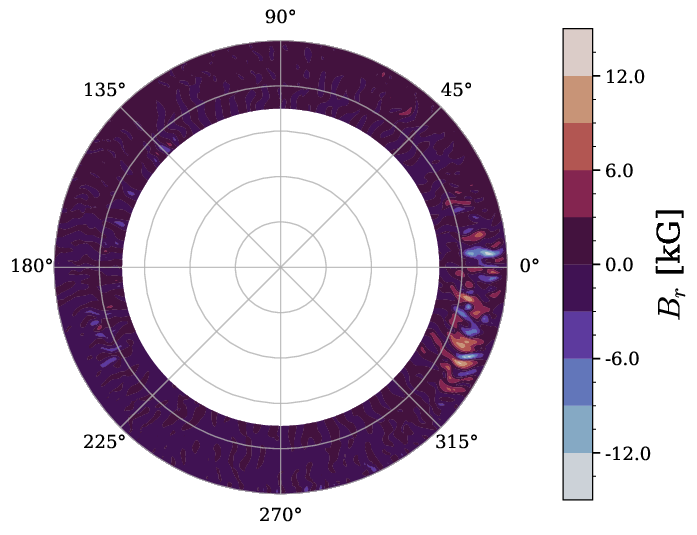
Figure 9: Radial magnetic field of Run B at the equator at $t=155$ yr. The $\hat{\bm{x}}$ and $\hat{\bm{y}}$ axes lie at $\phi=0^{\circ}$ and $\phi=90^{\circ}$, respectively. The $\hat{\bm{s}}$ and $\hat{\bm{s}}^{\prime}$ axes are obtained by performing clockwise rotations.

In this configuration, the nonaxisymmetric quadrupole moment is defined as $T=I_{s}-I_{s}^{\prime}$, where $I_{s}$ and $I_{s}^{\prime}$ are the moments of inertia about the $\hat{\bm{s}}$ and $\hat{\bm{s}}^{\prime}$ axes. The moment of inertia of the active star about the spin axis is $I_{p}=I_{xx}+I_{yy}$. The order of magnitude of the period variations can then be estimated as (Eq. 2 of Lanza, 2020)

$$\frac{T}{I_{p}}\approx\frac{4}{3}\left(\frac{M_{T}}{m_{S}}\right)\left(\frac{ma^{2}}{I_{p}}\right)\left(\frac{P}{P_{\rm mod}}\right)\left|\frac{\Delta P}{P}\right|,$$ (29)

where $M_{T}$ is the total mass of the binary, $m_{S}$ is the mass of the companion, $m$ is the reduced mass, $P$ is the orbital period, and $P_{\rm mod}$ is the modulation period. We take the density fields of Run B at $t=110$ yr and $t=155$ yr and compute the two quadrupole moments $T$ and $I_{p}$. By using Eq. (29) and the parameters of V471 Tau (see e.g., Hardy et al., 2015; Vaccaro et al., 2015) we can obtain an order of magnitude estimate of $\Delta P/P$. Fig. 10 shows the absolute value of the amplitude of the orbital period modulation as a function of separation angle $\alpha$ between $\hat{x}$ and $\hat{s}$ for $t=110$ yr (black dots) and $t=155$ yr (yellow triangles).

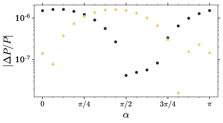
Figure 10: Absolute value of $\Delta P/P$ as a function of separation angle $\alpha$ between $\hat{\bm{x}}$ and $\hat{\bm{s}}$ for $t=110$ yr (black dots) and $t=155$ yr (yellow triangles).

$|\Delta P/P|$ ranges between $1.5\times 10^{-7}$ and $1.5\times 10^{-6}$, which contains the two contributions to the observed variations as well as their sum (Marchioni et al., 2018). From our simulations we get a value of $I_{p}$ that is of the same order of magnitude as in Lanza (2020), while $T$ is about one order of magnitude larger here. It is important to note that we have obtained $T$ based on a detailed 3D magneto-hydrodynamical simulation, while Lanza (2020) simply calculated which $T$ would be required to explain the observed ETVs.

In general, the gravitational potential felt by the companion can be written as (Applegate, 1992; Lanza, 2020)

$$\Phi=-\frac{GM}{r}-\frac{3G}{2r^{3}}\sum_{i,j}\frac{Q_{ij}x_{i}x_{j}}{r^{2}},$$ (30)

where $G$ is the gravitational constant, $M$ is the mass of the active star, $r$ is the distance between the center of the active star and the companion, $Q_{ij}$ is the quadrupole moment tensor, and ${\bm{x}}$ refers to Cartesian coordinates. Writing out the summation explicitly and expressing $x_{i}$ and $x_{j}$ in a spherical coordinate system $(r,\theta^{\prime},\phi^{\prime})$ with its origin coinciding with the center of the star, we arrive at

$$\Phi= -\frac{GM}{r}-\frac{3G}{2r^{3}}\biggl{\{}Q_{xx}\sin^{2}\theta^{\prime}\cos^{2}\phi^{\prime}$$

$$+Q_{yy}\sin^{2}\theta^{\prime}\sin^{2}\phi^{\prime}$$

$$+Q_{zz}\cos^{2}\theta^{\prime}$$

$$+2\biggl{(}Q_{xy}\sin^{2}\theta^{\prime}\cos\phi^{\prime}\sin\phi^{\prime}$$

$$+Q_{xz}\sin\theta^{\prime}\cos\theta^{\prime}\cos\phi^{\prime}$$

$$+Q_{yz}\sin\theta^{\prime}\cos\theta^{\prime}\sin\phi^{\prime}\biggr{)}\biggr{\}}.$$ (31)

The case of $\theta^{\prime}=\pi/2$ and $\phi^{\prime}=0$ is analogous to the assumptions that the rotation axis is perpendicular to the plane of the orbit and that the orbital motion is tidally locked, respectively. By assuming only the former, Eq. (4.3) is reduced to

$$\Phi= -\frac{GM}{r}-\frac{3G}{2r^{3}}\biggl{(}Q_{xx}\cos^{2}\phi^{\prime}$$

$$+Q_{yy}\sin^{2}\phi^{\prime}+2Q_{xy}\cos\phi^{\prime}\sin\phi^{\prime}\biggr{)}.$$ (32)

Here the effects of deviations from tidal locking can be modeled by making $\phi^{\prime}$ time-dependent. There are two alternatives, namely

$$\phi^{\prime}_{1} =\alpha\cos(\omega t),$$ (33)

$$\phi^{\prime}_{2} =\omega t.$$ (34)

In the former case, the companion is seen in the frame of reference of the rotating star as oscillating in the orbital plane with amplitude $\alpha$ and angular velocity $\omega$. In that case, $\phi^{\prime}_{1}$ corresponds to the analogous of the libration model. The latter expression for $\phi^{\prime}_{2}$ corresponds to the circulation model presented by Lanza (2020). This introduces two further contributions to the binary period variation that come from $Q_{yy}$ and $Q_{xy}$ (see Eq. 4.3). In Run B $Q_{yy}$ is, on average, the same as $Q_{xx}$. Meanwhile, $Q_{xy}$ is $10^{2}...10^{3}$ times smaller so it can be neglected. Thus,

$$\Phi=-\frac{GM}{r}-\frac{3G}{2r^{3}}\biggl{(}Q_{xx}\cos^{2}\phi^{\prime}+Q_{yy}\sin^{2}\phi^{\prime}\biggl{)}.$$ (35)

In contrast to previous studies, we can directly calculate each component of the gravitational quadrupole moment from our simulations. In this case it is advantageous to use Eqs. (4.3) and (4.3) rather than taking the limit of $\phi^{\prime}=0$. However, we would need to use new expressions to derive $\Delta P/P$ considering the libration and circulation models. Alternatively, it is also possible to try different values of $\alpha$ and $\omega$, and then directly solve Eq. (4.3) in a two-body simulation, which is however beyond the scope of the presented study. The influence of differences between $Q_{xx}$ and $Q_{yy}$ can be studied with N-body simulations by prescribing their time evolution and varying their amplitudes. It would be interesting to derive the parameters that can reproduce the observations and to compare them with our simulations.

5 Conclusions

We have presented three MHD simulations of stellar convection with different rotation rates, and studied the gravitational quadrupole moment and its connection to dynamo-generated magnetic fields. The analysis is based on a spherical harmonic decomposition of density and magnetic fields. Our results for Run B ($P=1.2$ days) show that a hemispheric dynamo mode can be an important ingredient for the eclipsing time variations in close binaries. This hemispheric dynamo produces equatorially asymmetric density variations and changes the moment of inertia along the rotation axis. The hemispheric activity migrates seemingly periodically between hemispheres and modulates the gravitational quadrupole moment. Furthermore, nonaxisymmetric magnetic fields modulate the other two diagonal components of the inertia tensor, adding a further modulation of $Q$. We also expect to have a further modulation of $Q$ that comes from the centrifugal force which will be included in a future work as it is the responsible for the angular momentum redistribution in the Applegate mechanism (Applegate, 1992). Linear correlation analysis confirms the role of the magnetic field in changing the quadrupole moment via density variations (Table 3) and the scatter plot between magnetic energy and quadrupole moment shows that large quadrupole moments are related to increased magnetic energy (see Fig. 6).

When our results are interpreted in the context of the classical Applegate mechanism, that is the star is tidally locked, then only the $Q_{xx}$ component of the quadrupole moment contributes to the period variations. In this scenario, we obtain orbital period modulations between one and two orders of magnitude smaller than observed in the target system V471 Tau (Marchioni et al., 2018). We emphasize that our results here should be taken with caution. We model the CZ of a Sun-like star while the CZ extends inward for less massive stars which are more common among PCEBs. It is yet to be investigated if large enough quadrupole moments are found in magnetohydrodynamical simulations of fully convective stars.

In the context of the models by Applegate (1989) and Lanza (2020), the order of magnitude estimate of the amplitude of the period modulation is $10^{-6}\ldots 10^{-7}$. This range encompasses the two observed contributions to the ${\rm O-C}$ diagram, as well as their combined effect. The observed period variations could be a combination of both, namely, both the axi- and nonaxisymmetric quadrupole moments contribute to them. The implication of the first interpretation is that there must be a hemispheric dynamo with an alternating active hemisphere in order to modulate $Q_{xx}$ as seen in our simulations. The second interpretation implies that the star is not tidally locked and that there is a nonaxisymmetric magnetic field in the CZ of the magnetically active star. We emphasize, however, given the caveats of the model such as imposed spherical symmetry, the coincidence in the order of magnitude between the ETVs, and in our model must be taken with caution. More importantly, relaxing the assumption of tidal locking leads to period variations that are between one and two orders of magnitude larger than in the tidal-locking scenario.

Observational studies suggest that both scenarios discussed, namely asymmetric magnetic fields and nontidally locked stars, are plausible. Firstly, a recent study by Klein et al. (2021) reported the reconstruction of the surface magnetic field of Proxima Centauri using Zeeman-Doppler imaging (ZDI). They found that the magnetic field is mainly poloidal with a dominant feature that is tilted at $51^{\circ}$ to the rotation axis (see their Figure 3) with a strength of $135$ G, that is a field distribution that is asymmetric with respect to the equator. This is a rather weak field so density fluctuations should be smaller than what we find in our simulations. However, Proxima Centauri is a slowly rotating M5.5 fully-convective star. The magnetic field strength of fully-convective stars increases with rotation until a saturation regime is reached, as measured by X-ray emission (see e.g., Wright & Drake, 2016), so density variations in magnetically active components of PCEBs are expected to be larger due to the increased magnetic field strength. This might also be the case for more evolved partially convective stars as a similar scaling property was recently found (Lehtinen et al., 2020). Studying the differences of stellar spots during a minima and maxima of of $O-C$ diagrams in PCEBs will provide direct evidence of the connection between the underlying dynamo and the orbital period variations. Secondly, the determination of tidal synchronization is equally important, as a deviation from synchronization results in a more complex relation between the gravitational quadrupole moment and eclipsing time variations and potentially larger binary period variations (see Lanza, 2020, and also Sect. 4.3 of this paper). Lurie et al. (2017) studied tidal synchronization of F, G, and K stars in short-period binaries. The authors find 21 eclipsing binaries that are not synchronized and argue that this could be explained either because they are young or have a complex dynamical history. Considering the dynamical evolution of PCEBs, where the secondary star is engulfed by the companion and spirals inwards toward the core of the more massive star (Paczynski, 1976), it is conceivable that they fall in this category.

The determination of the degree of synchronization in post common envelope binaries would be beneficial to further improve the understanding of the ETVs. The surface magnetic field distribution would be as equally important because such nonaxisymmetric fields produce larger quadrupole moments. Furthermore, there is also unexplored grounds in the simulations, such as the impact of the centrifugal force. Numerical models, specially for fully convective stars such as those in Käpylä (2021), that allow more freedom on the surface and near-surface layers of stars are desired as changes in the oblateness of the star can be captured.

Appendix A Scaling of the quadrupole moment with Mach number

In Navarrete et al. (2020) the scaling of the quadrupole moment was assumed to be

$$Q_{xx,{\rm phys}}\propto{\cal L}_{r}^{-2/3}Q_{xx,{\rm code}},$$ (36)

where $Q_{xx,{\rm phys}}$ is the physical quadrupole moment, and ${\cal L}_{r}$ is the ratio of simulation to solar luminosities at the bottom of the CZ, and $Q_{xx,{\rm code}}$ is the quadrupole moment in code units. Equivalently,

$$Q_{xx,{\rm phys}}\propto{\rm Ma}^{2}Q_{xx,{\rm code}},$$ (37)

where Ma is the Mach number. We test this scaling with two sets of simulations. Set L uses the same parameters as in Run B but we omit magnetic fields and rotation. Set M includes both rotation and magnetic fields. In particular, Run L2 has the same input parameters as Run B such as ${\cal L}_{r}$, but without rotation and magnetic fields. Relevant quantities are shown in Table 1. Run L2 produces a maximum variation of the quadrupole moment $\Delta Q_{xx}=6.8\times 10^{38}\,{\rm kg\,m}^{2}$, which is about 18 times smaller than in Run B. These variations develop on a timescale of 5 years and remain below the aforementioned level after that.

The rms value of the quadrupole moment fluctuations as a function of Mach number is shown in Fig. 11 for Set L and in Fig. 12 for Set M. The results are in reasonable agreement with the theoretical scaling, which is indicated by the dotted line in each plot.

Table 4: Parameters of sets L and M.

Run	$\mathfrak{F}_{r}$	Ma	$\Delta Q_{xx}^{\rm rms}$
L1	$2.74\times 10^{5}$	$5.67\times 10^{-2}$	$1.07\times 10^{-5}$
L2	$8.07\times 10^{5}$	$7.97\times 10^{-2}$	$2.85\times 10^{-5}$
L3	$2.34\times 10^{6}$	$1.11\times 10^{-1}$	$6.87\times 10^{-5}$
M1	$2.12\times 10^{5}$	$9.60\times 10^{-2}$	$3.44\times 10^{-5}$
M2	$6.37\times 10^{5}$	$1.25\times 10^{-1}$	$5.60\times 10^{-5}$
M3	$2.12\times 10^{6}$	$1.42\times 10^{-1}$	$9.30\times 10^{-5}$

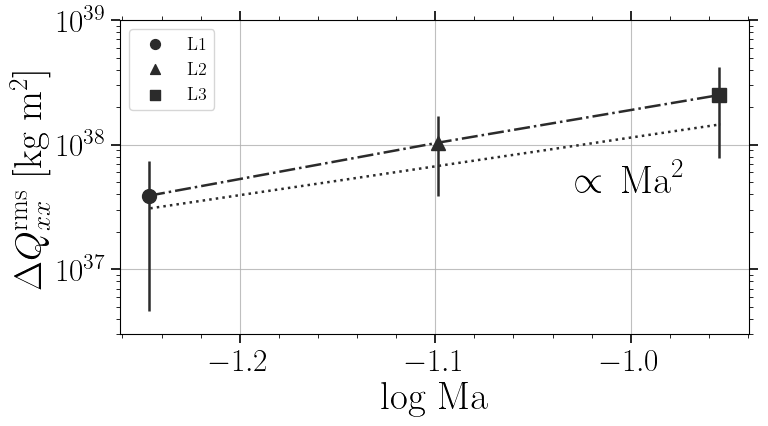
Figure 11: Root-mean-squared quadrupole moment fluctuations as a function of Mach number for Set L (without rotation and magnetic fields). The dotted line is proportional to the Mach number squared and the dash-dotted line joins the data points.

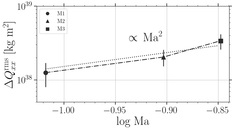
Figure 12: Root-mean-squared quadrupole moment fluctuations as a function of Mach number for Set M (with rotation and magnetic fields). The dotted line is proportional to the Mach number squared and the dash-dotted line joins the data points.

Appendix B Figures of the decomposed fields

References

- Applegate (1989) Applegate, J. H. 1989, ApJ, 337, 865
- Applegate (1992) Applegate, J. H. 1992, ApJ, 385, 621
- Brinkworth et al. (2006) Brinkworth, C. S., Marsh, T. R., Dhillon, V. S., & Knigge, C. 2006, MNRAS, 365, 287
- Brown et al. (2020) Brown, B. P., Oishi, J. S., Vasil, G. M., Lecoanet, D., & Burns, K. J. 2020, ApJ, 902, L3
- Busse (2002) Busse, F. H. 2002, Physics of Fluids, 14, 1301
- Cole et al. (2014) Cole, E., Käpylä, P. J., Mantere, M. J., & Brandenburg, A. 2014, ApJ, 780, L22
- Gastine et al. (2014) Gastine, T., Yadav, R. K., Morin, J., Reiners, A., & Wicht, J. 2014, MNRAS, 438, L76
- Grote & Busse (2000) Grote, E. & Busse, F. H. 2000, Phys. Rev. E, 62, 4457
- Hardy et al. (2015) Hardy, A., Schreiber, M. R., Parsons, S. G., et al. 2015, ApJ, 800, L24
- Käpylä (2021) Käpylä, P. J. 2021, A&A, 651, A66
- Käpylä et al. (2014) Käpylä, P. J., Käpylä, M. J., & Brandenburg, A. 2014, A&A, 570, A43
- Käpylä et al. (2010) Käpylä, P. J., Korpi, M. J., Brandenburg, A., Mitra, D., & Tavakol, R. 2010, Astronomische Nachrichten, 331, 73
- Käpylä et al. (2013) Käpylä, P. J., Mantere, M. J., Cole, E., Warnecke, J., & Brandenburg, A. 2013, ApJ, 778, 41
- Klein et al. (2021) Klein, B., Donati, J.-F., Hébrard, É. M., et al. 2021, MNRAS, 500, 1844
- Krause & Rädler (1980) Krause, F. & Rädler, K.-H. 1980, Mean-field magnetohydrodynamics and dynamo theory (Oxford, Pergamon Press, Ltd., 1980. 271 p.)
- Lanza (2020) Lanza, A. F. 2020, MNRAS, 491, 1820
- Lanza et al. (1998) Lanza, A. F., Rodono, M., & Rosner, R. 1998, MNRAS, 296, 893
- Lehtinen et al. (2020) Lehtinen, J. J., Spada, F., Käpylä, M. J., Olspert, N., & Käpylä, P. J. 2020, Nature Astronomy, 4, 658
- Lurie et al. (2017) Lurie, J. C., Vyhmeister, K., Hawley, S. L., et al. 2017, AJ, 154, 250
- Marchioni et al. (2018) Marchioni, L., Guinan, E. F., Engle, S. G., et al. 2018, Research Notes of the American Astronomical Society, 2, 179
- Navarrete et al. (2020) Navarrete, F. H., Schleicher, D. R. G., Käpylä, P. J., et al. 2020, MNRAS, 491, 1043
- Navarrete et al. (2021) Navarrete, F. H., Schleicher, D. R. G., Käpylä, P. J., et al. 2021, MNRAS, 504, 1676
- Navarrete et al. (2018) Navarrete, F. H., Schleicher, D. R. G., Zamponi Fuentealba, J., & Völschow, M. 2018, A&A, 615, A81
- Paczynski (1976) Paczynski, B. 1976, in IAU Symposium, Vol. 73, Structure and Evolution of Close Binary Systems, ed. P. Eggleton, S. Mitton, & J. Whelan, 75
- Pencil Code Collaboration et al. (2021) Pencil Code Collaboration, Brandenburg, A., Johansen, A., et al. 2021, The Journal of Open Source Software, 6, 2807
- Vaccaro et al. (2015) Vaccaro, T. R., Wilson, R. E., Van Hamme, W., & Terrell, D. 2015, ApJ, 810, 157
- Vanderbosch et al. (2017) Vanderbosch, Z. P., Clemens, J. C., Dunlap, B. H., & Winget, D. E. 2017, in Astronomical Society of the Pacific Conference Series, Vol. 509, 20th European White Dwarf Workshop, ed. P.-E. Tremblay, B. Gaensicke, & T. Marsh, 571–574
- Viviani et al. (2018) Viviani, M., Warnecke, J., Käpylä, M. J., et al. 2018, A&A, 616, A160
- Völschow et al. (2014) Völschow, M., Banerjee, R., & Hessman, F. V. 2014, A&A, 562, A19
- Völschow et al. (2018) Völschow, M., Schleicher, D. R. G., Banerjee, R., & Schmitt, J. H. M. M. 2018, A&A, 620, A42
- Völschow et al. (2016) Völschow, M., Schleicher, D. R. G., Perdelwitz, V., & Banerjee, R. 2016, A&A, 587, A34
- Wright & Drake (2016) Wright, N. J. & Drake, J. J. 2016, Nature, 535, 526
- Zorotovic & Schreiber (2013) Zorotovic, M. & Schreiber, M. R. 2013, A&A, 549, A95