Improving Lossless Compression Rates via Monte Carlo Bits-Back Coding

Abstract

Latent variable models have been successfully applied in lossless compression with the bits-back coding algorithm. However, bits-back suffers from an increase in the bitrate equal to the KL divergence between the approximate posterior and the true posterior. In this paper, we show how to remove this gap asymptotically by deriving bits-back coding algorithms from tighter variational bounds. The key idea is to exploit extended space representations of Monte Carlo estimators of the marginal likelihood. Naively applied, our schemes would require more initial bits than the standard bits-back coder, but we show how to drastically reduce this additional cost with couplings in the latent space. When parallel architectures can be exploited, our coders can achieve better rates than bits-back with little additional cost. We demonstrate improved lossless compression rates in a variety of settings, especially in out-of-distribution or sequential data compression.

1 Introduction

Datasets keep getting bigger; the recent CLIP model was trained on 400 million text-image pairs gathered from the internet (Radford et al., 2020). With datasets of this size coming from ever more heterogeneous sources, we need compression algorithms that can store this data efficiently.

In principle, data compression can be improved with a better approximation of the data generating distribution. Luckily, the quality of generative models is rapidly improving (van den Oord et al., 2016; Salimans et al., 2017; Razavi et al., 2019; Vahdat & Kautz, 2020). From this panoply of generative models, latent variable models are particularly attractive for compression applications, because they are typically easy to parallelize; speed is a major concern for compression methods. Indeed, some of the most successful learned compressors for large scale natural images are based on deep latent variable models (see Yang et al. (2020) for lossy, and Townsend et al. (2020) for lossless).

Lossless compression with latent variable models has a complication that must be addressed. Any model-based coder needs to evaluate the model’s probability mass function $p(x)$. Latent variable models are specified in terms of a joint probability mass function $p(x,z)$, where $z$ is a latent, unobserved variable. Computing $p(x)$ in these models requires a (typically intractable) summation, and achieving the model’s optimal bitrate, $-\log p(x)$, is not always feasible. When compressing large datasets of i.i.d. data, it is possible to approximate this optimal bitrate using the bits-back coding algorithm (Hinton & Van Camp, 1993; Townsend et al., 2019). Bits-back coding is based on variational inference (Jordan et al., 1999), which uses an approximation $q(z\,|\,x)$ to the true posterior $p(z\,|\,x)$. Unfortunately, this adds roughly $D_{\mathrm{KL}}(q(z\,|\,x)\,\|\,p(z\,|\,x))$ bits to the bitrate. This seems unimprovable for a fixed $q$, which is a problem, if approximating $p(z\,|\,x)$ is difficult or expensive.

Figure 1: Monte Carlo Bits-Back coders reduce the KL gap to zero.

In this paper, we show how to remove (asymptotically) the $D_{\mathrm{KL}}$ gap of bits-back schemes for (just about) any fixed $q$. Our method is based on recent work that derives tighter variational bounds using Monte Carlo estimators of the marginal likelihood (e.g., Burda et al., 2015). The idea is that $q$ and $p$ can be lifted into an extended latent space (e.g., Andrieu et al., 2010) such that the $D_{\mathrm{KL}}$ over the extended latent space goes to zero and the overall bitrate approaches $-\log p(x)$. For example, our simplest extended bits-back method, based on importance sampling, introduces $N$ identically distributed particles $z_{i}$ and a categorical random variable that picks from $z_{i}$ to approximate $p(z\,|\,x)$. We also define extended bits-back schemes based on more advanced Monte Carlo methods (AIS, Neal, 2001; SMC, Doucet et al., 2001).

Adding ${\mathcal{O}}(N)$ latent variables introduces another challenge that we show how to address. Bits-back requires an initial source of bits, and, naively applied, our methods increase the initial bit cost by ${\mathcal{O}}(N)$. One of our key contributions is to show that this cost can be reduced to ${\mathcal{O}}(\log N)$ for some of our coders using couplings in latent space, a novel technique that may be applicable in other settings to reduce initial bit costs. Most of our coders can be parallelized over the number of particles, which significantly reduces the computation overhead. So, our coders extend bits-back with little additional cost.

We test our methods in various lossless compression settings, including compression of natural images and musical pieces using deep latent variable models. We report between 2% - 19% rate savings in our experiments, and we see our most significant improvements when compressing out-of-distribution data or sequential data. We also show that our methods can be used to improve the entropy coding step of learned transform coders with hyperpriors (Ballé et al., 2018) for lossy compression. We explore the factors that affect the rate savings in our setting.

2 Background

2.1 Asymmetric Numeral Systems

The goal of lossless compression is to find a short binary representation of the outcome of a discrete random variable $x\sim p_{d}(x)$ in a finite symbol space $x\in{\mathbb{S}}$. Achieving the best possible expected length, i.e., the entropy $H(p_{d})$ of $p_{d}$, requires access to $p_{d}$, and typically a model probability mass function (PMF) $p(x)$ is used instead. In this case, the smallest achievable length is the cross-entropy of $p$ relative to $p_{d}$, $H(p_{d},p)=-\sum_{x}p_{d}(x)\log p(x)$. See MacKay (2003); Cover & Thomas (1991) for more detail.

Asymmetric numeral systems (ANS) are model-based coders that achieve near optimal compression rates on sequences of symbols (Duda, 2009). ANS stores data in a stack-like ‘message’ data structure, which we denote $m$, and provides an inverse pair of functions, $\mathrm{encode}_{p}$ and $\mathrm{decode}_{p}$, which each process one symbol $x\in{\mathbb{S}}$ at a time:

$$\mathrm{encode}_{p}:m,x\mapsto m^{\prime}$$ (1)

$$\mathrm{decode}_{p}:m^{\prime}\mapsto(m,x).$$

Encode pushes $x$ onto $m$, and decode pops $x$ from $m^{\prime}$. Both functions require access to routines for computing the cumulative distribution function (CDF) and inverse CDF of $p$. If $n$ symbols, drawn i.i.d. from $p_{d}$, are pushed onto $m$ with $p$ , the bitrate (bits/symbol) required to store the ANS message approaches $H(p_{d},p)+\epsilon$ for some small error $\epsilon$ (Duda, 2009; Townsend, 2020). The exact sequence is recovered by popping $n$ symbols off the final $m$ with $p$.

For our purposes, the ANS message can be thought of as a store of randomness. Given a message $m$ with enough bits, regardless of $m$’s provenance, we can decode from $m$ using any distribution $p$. This will return a random symbol $x$ and remove roughly $-\log p(x)$ bits from $m$. Conversely, we can encode a symbol $x$ onto $m$ with $p$, which will increase $m$’s length by roughly $-\log p(x)$. If a sender produces a message $m$ through some sequence of encode or decode steps using distributions $p_{i}$, then a receiver, who has access to the $p_{i}$, can recover the sequence of encoded symbols and the initial message by reversing the order of operations and switching encodes with decodes. When describing algorithms, we often leave out explicit references to $m$, instead writing steps like ‘$\mathrm{encode}\ x$ with $p(x)$’. See Fig. 2.

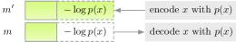
Figure 2: ANS is a last-in-first-out lossless coder. We adopt the visualizations of (Kingma et al., 2019): the green bars represent the message $m$, a stack that stores symbols $x$.

2.2 Bits-Back Compression with ANS

The class of latent variable models is highly flexible, and most operations required to compute with such models can be parallelized, making them an attractive choice for model-based coders. Bits-back coders, in particular Bits-Back with ANS (BB-ANS, Townsend et al., 2019), specialize in compression using latent variable models.

A latent variable model is specified in terms of a joint distribution $p(x,z)$ between $x$ and a latent discrete random variable taking value in a symbol space $z\in{\mathbb{S}}^{\prime}$. We assume that the joint distribution of latent variable models factorizes as $p(z)p(x\,|\,z)$ and that the PMFs, CDFs, and inverse CDFs, under $p(z)$ and $p(x\,|\,z)$ are tractable. However, computing the marginal $p(x)=\sum_{z}p(z)p(x\,|\,z)$ is often intractable. This fact means that we cannot directly encode $x$ onto $m$. A naive strategy would be for the sender to pick some $z\in{\mathbb{S}}^{\prime}$, and encode $(x,z)$ using $p$, which would require $-\log p(x,z)$ bits; however, this involves communicating the symbol $z$, which is redundant information.

BB-ANS gets a better bitrate, by compressing sequences of symbols in a chain and by having the sender decode latents $z$ from the intermediate message state, rather than picking $z$; see Fig. 3. Suppose that we have already pushed some symbols onto a message $m$. BB-ANS uses an approximate posterior $q(z\,|\,x)$ such that if $p(x,z)=0$ then $q(z\,|\,x)=0$. To encode a symbol $x$ onto $m$, the sender first pops $z$ from $m$ using $q(z\,|\,x)$. Then they push $(x,z)$ onto $m$ using $p(x,z)$. The new message $m^{\prime}$ has approximately $-\log p(x,z)+\log q(z\,|\,x)$ more bits than $m$. $m^{\prime}$ is then used in exactly the same way for the next symbol. The per-symbol rate saving over the naive method is $-\log q(z\,|\,x)$ bits. However, for the first symbol, an initial message is needed, causing a one-time overhead.

2.3 The Bitrate of Bits-Back Coders

When encoding a sequence of symbols, we define the total bitrate to be the number of bits in the final message per symbol encoded; the initial bits to be the number of bits needed to initialize the message; and the net bitrate to be the total bitrate minus the initial bits per symbol, which is equal to the expected increase in message length per symbol. As the number of encoded symbols grows, the total bitrate of BB-ANS will converge to the net bitrate.

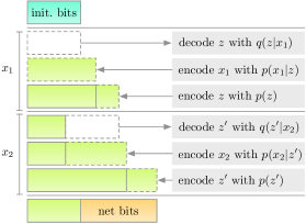
Figure 3: Encoding $(x_{1},x_{2})$ requires an initial source of bits (light blue), but bits-back reduces its total bit consumption by using intermediate messages as the initial source of bits for encoding $x_{2}$. The net bits used (light orange) is close to the negative ELBO.

One subtlety is that the BB-ANS bitrate depends on the distribution of the latent $z$, popped with $q(z\,|\,x)$. In an ideal scenario, where $m$ contains i.i.d. uniform Bernoulli distributed bits, $z$ will be an exact sample from $q$. Unfortunately, in practical situations, the exact distribution of $z$ is difficult to characterize. Nevertheless, Townsend et al. (2019) found the ‘evidence lower bound’ (ELBO)

$$\operatorname{\mathbb{E}}_{z\sim q(z\,|\,x)}\left[-\log p(x,z)+\log q(z\,|\,x)\right]$$ (2)

$$=-\log p(x)+D_{\mathrm{KL}}(q(z\,|\,x)\,\|\,p(z\,|\,x)),$$

which assumes $z\sim q(z\,|\,x)$, to be an accurate predictor of BB-ANS’s empirical compression rate; the effect of inaccurate samples (which they refer to as ‘dirty bits’) is typically less than $1\%$. So, in this paper we mostly elide the dirty bits issue, regarding (2) to be the net bitrate of BB-ANS, and hereafter we refer to vanilla BB-ANS as BB-ELBO. Taking the expectation under $p_{d}$, BB-ELBO achieves a net bitrate of approximately $H(p_{d},p)+\mathbb{E}_{x\sim p_{d}}[D_{\mathrm{KL}}(q(z\,|\,x)\,\|\,p(z\,|\,x))]$.

Algorithm 1 Extended Latent Space Representation of Importance Sampling

Process $Q({\mathcal{Z}}\,|\,x)$

       sample $\{z_{i}\}_{i=1}^{N}\sim\prod_{i=1}^{N}q(z_{i}\,|\,x)$
compute $\tilde{w}_{i}\propto\frac{p(x,z_{i})}{q(z_{i}\,|\,x)}$
sample $j\sim\operatorname{Cat}\left(\tilde{w}_{j}\right)$
return $\{z_{i}\}_{i=1}^{N},j$

Process $P(x,{\mathcal{Z}})$

       sample $j\sim\operatorname{Cat}(1/N)$
sample $z_{j}\sim p(z_{j})$
sample $x\sim p(x\,|\,z_{j})$
sample $\{z_{i}\}_{i\neq j}\sim\prod_{i\neq j}q(z_{i}\,|\,x)$
return $x,\{z_{i}\}_{i=1}^{N},j$

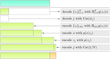
(a) Bits-Back Importance Sampling (BB-IS)

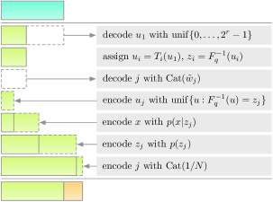
(b) Bits-Back Coupled Importance Sampling (BB-CIS)

Figure 4: The initial bit cost of encoding a single symbol $x$ with IS-based coders is reduced from ${\mathcal{O}}(N)$ to ${\mathcal{O}}(\log N)$ by coupling the latents with shared randomness. Both of these coders achieve a net bitrate that approaches $-\log p(x)$ as $N\to\infty$.

3 Monte Carlo Bits-Back Coding

The net bitrate of bits-back is ideally the negative ELBO. This rate seems difficult to improve without finding a better $q$. However, the ELBO may be a loose bound on the marginal log-likelihood. Recent work in variational inference shows how to bridge the gap from the ELBO to the marginal log-likelihood with tighter variational bounds (e.g., Burda et al., 2015; Domke & Sheldon, 2018), motivating the question: can we derive bits-back coders from those tighter bounds and approach the cross-entropy?

In this section we provide an affirmative answer to this question with a framework called Monte Carlo bits-back coding (McBits). We point out that the extended space constructions of Monte Carlo estimators can be reinterpreted as bits-back coders. One of our key contributions is deriving variants whose net bitrates improve over BB-ELBO, while being nearly as efficient with initial bits. We begin by motivating our framework with two worked examples. Implementation details are in Appendix A.

3.1 Bits-Back Importance Sampling

The simplest of our McBits coders is based on importance sampling (IS). IS samples $N$ particles $z_{i}\sim q(z_{i}\,|\,x)$ i.i.d. and uses the importance weights $p(x,z_{i})/q(z_{i}\,|\,x)$ to estimate $p(x)$. The corresponding variational bound (IWAE, Burda et al., 2015) is the log-average importance weight:

$$-\mathbb{E}_{\{z_{i}\}_{i=1}^{N}}\left[\log\left(\sum_{i=1}^{N}\frac{1}{N}\frac{p(x,z_{i})}{q(z_{i}\,|\,x)}\right)\right]\geq-\log p(x).$$ (3)

IS provides a consistent estimator of $p(x)$. If the importance weights are bounded, the left-hand side of equation (3) converges monotonically to $-\log p(x)$ (Burda et al., 2015).

Surprisingly, equation (3) is actually the evidence lower bound between a different model and a different approximate posterior on an extended space (Andrieu et al., 2010; Cremer et al., 2017; Domke & Sheldon, 2018). In particular, consider an expanded latent space ${\mathbb{S}}^{\prime N}\times\{1\ ..\ N\}$ that includes the configurations of the $N$ particles $\{z_{i}\}_{i=1}^{N}$ and an index $j\in\{1\ ..\ N\}$. The left-hand side of equation (3) can be re-written as the (negative) ELBO between a pair of distributions $P$ and $Q$ defined over this extended latent space, which are given in Alg. 1. Briefly, given $x$, $Q$ samples $N$ particles $z_{i}\sim q(z_{i}\,|\,x)$ i.i.d. and selects one of them by sampling an index $j$ with probability $\tilde{w}_{j}\propto p(x,z_{j})/q(z_{j}\,|\,x)$. The distribution $P$ pre-selects the special $j$th particle uniformly at random, samples its value $z_{j}\sim p(z_{j})$ from the prior of the underlying model, and samples $x\sim p(x\,|\,z_{j})$ given $z_{j}$. The remaining $z_{i}\sim q(z_{i}\,|\,x)$ for $i\neq j$ are sampled from the underlying approximate posterior. Because $P$ and $Q$ use $q$ for all but the special $j$th particle, most of the terms in the difference of the log-mass functions cancel, and all that remains is equation (3). See Appendix A.4.

Once we identify the left-hand side of equation (3) as a negative ELBO over the extended space, we can derive a bits-back scheme that achieves an expected net bitrate equal to equation (3). We call this the Bits-Back Importance Sampling (BB-IS) coder, and it is visualized in Fig. 4(a). To encode a symbol $x$, we first decode $N$ particles $z_{i}$ and the index $j$ with the $Q$ process by translating each ‘sample’ to ‘decode’. Then we encode $x$, the particles $z_{i}$, and the index $j$ jointly with the $P$ process by translating each ‘sample’ to ‘encode’ in reverse order. By reversing $P$ at encode time, we ensure that receiver decodes with $P$ in the right order.

Thus, ignoring the clean bits question, BB-IS’s asymptotic net bitrate is close to the left-hand side of equation (3), which converges to the marginal log-likelihood (Burda et al., 2015). Ultimately, as $N\to\infty$, it reaches the cross-entropy.

3.2 Bits-Back Coupled Importance Sampling

Unfortunately, the BB-IS coder requires roughly $-\log\tilde{w}_{j}-\sum_{i=1}^{N}\log q(z_{i}\,|\,x)\in{\mathcal{O}}(N)$ initial bits. The reason is that each decoded random variable needs to remove some bits from $m$. Can this be avoided? Here, we design Bits-Back Coupled Importance Sampling (BB-CIS), which achieves a net bitrate comparable to BB-IS while reducing the initial bit cost to ${\mathcal{O}}(\log N)$. BB-CIS achieves this by decoding a single common random number, which is shared by the $z_{i}$. The challenge is showing that a net bitrate comparable to BB-IS is still achievable under such a reparameterization.

BB-CIS is based on a reparameterization of the particles $z_{i}$ as deterministic functions of coupled uniform random variables. The method is a discrete analog of the inverse CDF technique for simulating non-uniform random variates (Devroye, 2006). Specifically, suppose that the latent space ${\mathbb{S}}^{\prime}$ is totally ordered, and the probabilities of $q$ are approximated to an integer precision $r>0$, i.e., $2^{r}q(z\,|\,x)$ is an integer for all $z\in{\mathbb{S}}^{\prime}$. Define the function $F_{q}^{-1}:\{0\ ..\ 2^{r}-1\}\to{\mathbb{S}}^{\prime}$,

$$F_{q}^{-1}(u)=\arg\min\left\{z:\sum\nolimits_{z^{\prime}\leq z}2^{r}q(z^{\prime}\,|\,x)>u\right\}.$$ (4)

$F^{-1}_{q}$ maps the uniform samples into samples from $q$. This is visualized in Fig. 5. A coupled set of particles $z_{i}$ with marginals $q(z_{i}\,|\,x)$ can be simulated with a common random number by sampling a single uniform $u$ and setting $z_{i}=F_{q}^{-1}(T_{i}(u))$ for some functions $T_{i}:\{0\ ..\ 2^{r}-1\}\to\{0\ ..\ 2^{r}-1\}$, as in Fig. 6. Intuitively, $T_{i}$ maps $u$ to the uniform $u_{i}$ underlying $z_{i}$. To ensure that $z_{i}$ have the same marginal, we require that $T_{i}$ are bijective functions. For example, $T_{i}$ can be defined as a fixed ‘shift’ by integer $k_{i}$ , i.e., $T_{i}(u)=(u+k_{i})\ \mathrm{mod}\ 2^{r}$ with inverse $T_{i}^{-1}(u)=(u-k_{i})\ \mathrm{mod}\ 2^{r}$. We set $T_{1}(u)=u$ by convention.

Figure 5: Mapping uniforms in $\{0\ ..\ 2^{r}-1\}$ to samples in ${\mathbb{S}}^{\prime}$. Colors represent the subsets mapped to $z$ of size $2^{r}q(z\,|\,x)$.

BB-CIS uses these couplings in a latent decoding process that saves initial bits. It decodes $u_{1}$ from $m$ with $\operatorname{unif}\{0\ ..\ 2^{r}-1\}$, sets $z_{i}=F_{q}^{-1}(T_{i}(u_{1}))$, and decodes the index $j$ of the special particle $z_{j}$ with $\operatorname{Cat}(\tilde{w}_{j})$. This reduces the initial bit cost to $r-\log\tilde{w}_{j}\in{\mathcal{O}}(1)+{\mathcal{O}}(\log N)={\mathcal{O}}(\log N)$. Note that the ${\mathcal{O}}(\log N)$ term is for decoding the index $j$ which does not scale with latent dimension, thus the ${\mathcal{O}}(1)$ term dominates for high dimensional latents. Also, in the ANS implementation, all compressed message lengths are rounded to a multiple of a specified precision (e.g., 16) which may mask small changes caused by the ${\mathcal{O}}(\log N)$ term. Thus, in practice, BB-CIS demonstrates a nearly constant initial bits cost (Fig. 8(c)).

The coupled latent decoding process needs to be matched with an appropriate encoding process for $x$. Suppose that we finished encoding $x$, as with BB-IS, by encoding $\{z_{i}\}_{i\neq j}$ with $q(z_{i}\,|\,x)$ i.i.d. and encoding $(x,z_{j},j)$ with $p(x,z_{j})/N$. The net bitrate would be

$$\operatorname{\mathbb{E}}_{u_{1}}\left[-r-\sum_{i=1}^{N}\log q(z_{i}\,|\,x)-\log\left(\sum_{i=1}^{N}\frac{1}{N}\frac{p(x,z_{i})}{q(z_{i}\,|\,x)}\right)\right].$$

This is clearly worse than BB-IS. The culprits are the $N-1$ latents that BB-IS pushes onto $m$, which is wasteful, because they are deterministically coupled. Fundamentally, the encoding process of BB-IS is not balanced with the initial bit savings of our coupled latent decoding process.

The solution is to design an encoding process over $\{z_{i}\}_{i=1}^{N}$, $\{u_{i}\}_{i=1}^{N}$, and $x$, which exactly matches the initial bit savings of the coupled decoding process. The idea is to encode just $(u_{j},x,z_{j},j)$, which is enough information for the receiver to reconstruct all other variables. The key is to design the encoding for $u_{j}$. Encoding $u_{j}$ with a uniform on $\{0\ ..\ 2^{r}-1\}$ is unnecessarily wasteful, because $z_{j}$ restricts the range of $u_{j}$. It turns out, that the best we can do is to encode $u_{j}$ with $\operatorname{unif}\{u:F^{-1}_{q}(u)=z_{j}\}$. Finally $(x,z_{j},j)$ are encoded with $p(x,z_{j})/N$. BB-CIS’s encode is given in Fig. 4(b).

Figure 6: BB-CIS only needs to decode a single random uniform $u$ and then applies bijections $T_{i}$ to produce the uniforms $u_{i}$ underlying $z_{i}$. We set $T_{1}(u)=u$ by convention.

BB-CIS has the following expected net bitrate:

$$-\operatorname{\mathbb{E}}_{u_{1}}\left[\log\left(\sum_{i=1}^{N}\frac{1}{N}\frac{p(x,z_{i})}{q(z_{i}\,|\,x)}\right)\right].$$ (5)

Thus, BB-CIS achieves a net bitrate comparable to BB-IS, but uses only ${\mathcal{O}}(\log N)$ initial bits. We show this in Appendix A.5. We also show that the BB-CIS net bitrate can be interpreted as a negative ELBO over an extended latent space, which accounts for the configurations of $z_{i},u_{i},$ and $j$. This extended space construction is novel, and we believe it may be useful for deriving other coupling schemes that reduce initial bit consumption. Common random numbers are classical tools in Monte Carlo methods; in bits-back they may serve as a tool for controlling initial bit cost.

The net bitrate of BB-CIS can fail to converge to $-\log p(x)$, if the $T_{i}$ are poorly chosen. In our experiments, we used fixed (but randomly chosen) shifts shared between the sender and receiver. This scheme converged as quickly as BB-IS in terms of net bitrate, but at a greatly reduced total bitrate. However, we point out that further work is required to explore more efficient bijections in terms of computation cost and compression performance.

3.3 General Framework

Monte Carlo bits-back coders generalize these two examples. They are bits-back coders built from extended latent space representations of Monte Carlo estimators of the marginal likelihood. Let $\hat{p}_{N}(x)$ be a positive unbiased Monte Carlo estimator of the marginal likelihood that can be simulated with ${\mathcal{O}}(N)$ random variables, i.e., $\operatorname{\mathbb{E}}[\hat{p}_{N}(x)]=p(x)$. Importance sampling is the quintessential example, $\hat{p}_{N}(x)=N^{-1}\sum_{i=1}^{N}p(x,z_{i})/q(z_{i}\,|\,x)$, but more efficient estimators of $p(x)$ can be built using techniques like annealed importance sampling (Neal, 2001) or sequential Monte Carlo (Doucet et al., 2001).

A variational bound on the log-marginal likelihood can be derived from $\hat{p}_{N}(x)$ by Jensen’s inequality,

$$-\operatorname{\mathbb{E}}[\log\hat{p}_{N}(x)]\geq-\log p(x).$$ (6)

If $\hat{p}_{N}(x)$ is strongly consistent in $N$ (as is the case with many of these estimators) and $-\log\hat{p}_{N}(x)$ satisfies a uniform integrability condition, then $-\operatorname{\mathbb{E}}[\log\hat{p}_{N}(x)]\to-\log p(x)$ (Maddison et al., 2017). This framework captures recent efforts on tighter variational bounds (Burda et al., 2015; Maddison et al., 2017; Naesseth et al., 2018; Le et al., 2018; Domke & Sheldon, 2018; Caterini et al., 2018).

As with BB-IS and BB-CIS, the key step in the McBits framework is to identify an extended latent space representation of $\hat{p}_{N}(x)$. Let ${\mathcal{Z}}\sim Q({\mathcal{Z}}\,|\,x)$ be a set of random variables (often including those needed to compute $\hat{p}_{N}(x)$). If there exists a ‘target’ probability distribution $P(x,\mathcal{Z})$ over $x$ and ${\mathcal{Z}}$ with marginal $p(x)$ such that

$$\hat{p}_{N}(x)=\frac{P(x,\mathcal{Z})}{Q(\mathcal{Z}\,|\,x)},$$ (7)

then the McBits coder, which decodes ${\mathcal{Z}}$ with $Q({\mathcal{Z}}\,|\,x)$ and encodes $(x,{\mathcal{Z}})$ with $P(x,{\mathcal{Z}})$, will achieve a net bitrate of $-\log\hat{p}_{N}(x)$. In particular, if the log estimator converges in expectation to the log-marginal likelihood and we ignore the dirty bits issue, then $D_{\mathrm{KL}}(Q({\mathcal{Z}}\,|\,x)\,\|\,P({\mathcal{Z}}\,|\,x))\to 0$ and the McBits coder will achieve a net bitrate of $H(p_{d},p)$.

The challenge is to identify ${\mathcal{Z}}$, $Q$, and $P$. While Monte Carlo estimators of $p(x)$ get quite elaborate, many of them admit such extended latent space representations (e.g., Neal, 2001; Andrieu et al., 2010; Finke, 2015; Domke & Sheldon, 2018). These constructions are techniques for proving the unbiasedness of the estimators; one of our contributions is to demonstrate that they can become efficient bits-back schemes. In Appendix A, we provide pseudocode and details for all McBits coders.

Bits-Back Annealed Importance Sampling (BB-AIS)

Annealed importance sampling (AIS) is a generalization of importance sampling, which introduces a path of $N$ intermediate distributions between the base distribution $q(z\,|\,x)$ and the unnormalized posterior $p(z\,|\,x)$. AIS samples a sequence of latents by iteratively applying MCMC transition kernels that leave each intermediate distributions invariant. By bridging the gap between $q(z\,|\,x)$ and $p(z\,|\,x)$, AIS’s estimate of $p(x)$ typically converges faster than importance sampling (Neal, 2001). The corresponding McBits coder, BB-AIS, requires ${\mathcal{O}}(N)$ initial bits, but this can be addressed with the BitSwap trick (Kingma et al., 2019), which we call BB-AIS-BitSwap. Another issue is that the intermediate distributions are usually not factorized, which makes it challenging to work with high-dimensional $z$.

Bits-Back Sequential Monte Carlo (BB-SMC)

Sequential Monte Carlo (SMC) is a particle filtering method that combines importance sampling with resampling. Its estimate of $p(x)$ typically converges faster than importance sampling for time series models (Cérou et al., 2011; Bérard et al., 2014). SMC maintains a population of particles. At each time step, the particles independently sample an extension from the proposal distribution. Then the whole population is resampled with probabilities in proportion to importance weights. The corresponding McBits coder, BB-SMC, requires ${\mathcal{O}}(TN)$ initial bits, where $T$ is the length of the time series. We introduce a coupled variant, BB-CSMC, in the appendix that reduces this to ${\mathcal{O}}(T\log N)$.

Computational Cost

All of our coders require ${\mathcal{O}}(N)$ computational cost, but the IS- and SMC-based coders are amenable to parallelization over particles. In particular, we implemented an end-to-end parallelized version of BB-IS based on the JAX framework (Bradbury et al., ) and benchmarked on compressing the binarized MNIST dataset with one-layer VAE model. As shown in Fig. 7, the computation time scales sublinearly with the number of particles, which demonstrates the potential practicality of our method, in some settings, with hundreds of particles. Detailed discussion is in Appendix LABEL:appendix:compcost.

Figure 7: BB-IS total encode + decode time for binarized MNIST scales very well with $N$ using a parallel implementation of ANS. BB-ELBO ($N=1$) uses a simpler code-base, which runs faster. The experiment was run on a Tesla P100 GPU with 12GB of memory, together with an Intel Xeon Silver 4110 CPU at 2.10GHz.

(a) As $N\to\infty$, the net bitrate converges to the entropy for most coders on the toy mixture model.

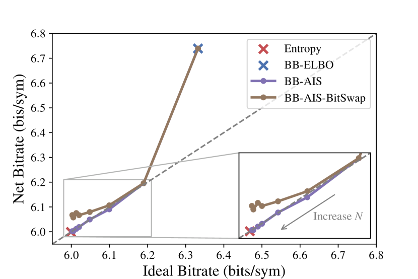
(b) As $N\to\infty$, the net bitrate converges. Convergence to the ideal bitrate (dashed line) indicates clean bits.

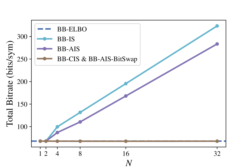
(c) The initial bit cost (reflected in the total bitrate after the first symbol) is controlled by some McBits coders, but not others.

Figure 8: The bitrate of McBits coders converges (in the number of particles $N$) to the entropy when using the data generating distribution. The initial bit cost of naive coders scales like ${\mathcal{O}}(N)$, but coupled and BitSwap variants significantly reduce it. Bitrates are bits/sym.

4 Related Work

Recent work on learned compressors considers two classes of deep generative models: models based on normalizing flows (Rippel & Adams, 2013; Dinh et al., 2014, 2016; Rezende & Mohamed, 2015) and deep latent variable models (Kingma & Welling, 2013; Rezende et al., 2014). Flow models are generally computationally expensive, and optimizing a function with discrete domain and codomain using gradient descent can be cumbersome. Despite these issues, flow models are the state of the art for lossless compression of small images (van den Berg et al., 2020).

‘Bits-back’ was originally meant to provide an information theoretic basis for approximate Bayesian inference methods (Wallace, 1990; Hinton & Van Camp, 1993; Frey & Hinton, 1997; Frey, 1998). Townsend et al. (2019) showed that the idea can lead directly to a practical compression algorithm for latent variable models. Follow up work reduced the initial bit cost for hierarchical models (Kingma et al., 2019), and extended it to large scale models and larger images (Townsend et al., 2020). For lossy compression, the variational autoencoder framework is a natural fit for training transform coders (Johnston et al., 2019; Ballé et al., 2016, 2018; Minnen et al., 2018; Yang et al., 2020).

Relative entropy coding (REC, Havasi et al., 2019; Flamich et al., 2020) is an alternative coding scheme for latent variable models that seeks to address the initial bits overhead in bits-back schemes. However, practical REC implementations require a particular reparameterization of the latent space, and it is unclear whether the REC latent structure is compatible with the extended latents in McBits.

5 Experiments

We studied the empirical properties and performance of our McBits coders on both synthetic data and practical image and music piece compression tasks. Many of our experiments used continuous latent variable models and we adopted the maximum entropy quantization in Townsend et al. (2019) to discretize the latents. We sometimes evaluated the ideal bitrate, which for each coder is the corresponding variational bound estimated with pseudorandom numbers. For continuous latent variable models, the ideal bitrate does not account for quantization. We rename BB-ANS to BB-ELBO. $N$ refers to the number of intermediate distributions for BB-AIS. Details are in Appendix LABEL:appendix:experimental_details. Our implementation is available at https://github.com/ryoungj/mcbits.

5.1 Lossless Compression on Synthetic Data

We assessed the convergence properties, impact of dirty bits, and initial bit cost of our McBits coders on synthetic data. First, a dataset of 5000 symbols was generated i.i.d. from a mixture model with alphabet sizes 64 and 256 for the observations and latents, respectively. BB-ELBO, BB-IS, BB-CIS, and BB-AIS were evaluated using the true data generating distribution with a uniform approximate posterior, ensuring a large mismatch with the true posterior. For BB-AIS, a Metropolis–Hastings kernel with a uniform proposal was used. The bijective operators of BB-CIS applied randomly selected, but fixed, shifts to the sampled uniform.

The net bitrates of BB-IS, BB-CIS, and BB-AIS converged to the entropy (optimal rate) as the number of particles increased. This is shown in 8(a). The indistinguishable gap between BB-CIS and BB-IS illustrates that particle coupling did not lead to a deterioration of net bitrate. BB-AIS-BitSwap did not converge, likely due to the dirty bits issue.

We measured the impact of dirty bits by plotting ideal versus net bitrates in Fig. 8(b). The deviation of any point to the dashed line indicates the severity of dirty bits. Interestingly, most of our McBits coders appeared to ‘clean’ the bitstream as $N$ increased, i.e. the net bitrate converged to the entropy, as shown in Fig. 8(b) for BB-AIS and in Fig. LABEL:fig:cleanliness_plot_toy_mixture_all in Appendix LABEL:appendix:lossless_toy for all coders. Only BB-AIS-BitSwap did not clean the bitstream (Fig. 8(b)), indicating that the order of operations has a significant impact on the cleanliness of McBits coders.

We quantified the initial bits cost by computing the total bitrate after the first symbol. As shown in Fig. 8(c), it increased linearly with $N$ for BB-IS and BB-AIS, but remained fixed for BB-CIS and BB-AIS-BitSwap.

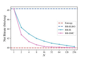
Figure 9: As $N\rightarrow\infty$, the net bitrates of BB-IS and BB-SMC converge to the entropy on the toy HMM, but BB-SMC converges much faster.

Our second experiment was with a dataset of 5000 symbol subsequences generated i.i.d. from a small hidden Markov model (HMM). We used 10 timesteps with alphabet sizes 16 and 32 for the observations and latents, respectively. BB-ELBO, BB-IS, and BB-SMC were evaluated using the true data generating distribution and a uniform approximate posterior. The net bitrates of BB-IS and BB-SMC converged to the entropy, but BB-SMC converged much faster, illustrating the effectiveness of resampling particles for compressing sequential data (Fig. 9).

5.2 Lossless Compression on Images

We benchmarked the performance of BB-IS and BB-CIS on the standard train-test splits of two datasets: an alphanumeric extension of MNIST called EMNIST (Cohen et al., 2017), and CIFAR-10 (Krizhevsky, 2009). EMNIST was dynamically binarized following Salakhutdinov & Murray (2008), and a VAE with 1 stochastic layer was used as in Burda et al. (2015). For CIFAR-10, we used VQ-VAE (Oord et al., 2017) with discrete latent variables and trained with continuous relaxations (Sønderby et al., 2017).

Table 1: BB-IS performs better on models that were trained with the same number of particles. The net bitrates (bits/dim) of BB-IS on EMNIST-MNIST and CIFAR-10 test sets. $N=50$ for EMNIST-MNIST and $N=10$ for CIFAR-10.

	MNIST		CIFAR-10
	ELBO	IWAE	ELBO	IWAE
BB-ELBO	0.236	0.236	4.898	4.898
BB-IS (5)	0.232	0.231	4.866	4.827
BB-IS ($N$)	0.230	0.228	4.857	4.810
Savings	2.5%	3.4%	0.8%	1.8%

Table 2: BB-IS leads to more improved compression rates in out-of-distribution compression settings. The net bitrates (bits/dim) of BB-IS on EMNIST test sets using a VAE.

Trained on	MNIST		Letters
Compressing	MNIST	Letters	MNIST	Letters
BB-ELBO	0.236	0.310	0.257	0.250
BB-IS (5)	0.231	0.289	0.249	0.243
BB-IS (50)	0.228	0.280	0.244	0.239
Savings	3.4%	9.7%	5.1%	4.4%

The variational bounds used to train the VAEs had an impact on compression performance. When using BB-IS with a model trained on the IWAE objective, equalizing the number of particles during compression and training resulted in better rates than BB-IS with an ELBO-trained VAE (Table 1). Therefore, we always use our McBits coders with models trained on the corresponding variational bound.

We assessed BB-IS in an out-of-distribution (OOD) compression setting. We trained models on standard EMNIST-Letters and EMNIST-MNIST splits and evaluated compression performance on the test sets. BB-IS achieved greater rate savings than BB-ELBO when transferred to OOD data (Table 2). This illustrates that BB-IS may be particularly useful in more practical compression settings where the data distribution is different from that of the training data.

Table 3: BB-CIS achieves the best total bitrates compared to baselines on EMNIST test sets.

Method	MNIST	Letters
PNG	0.819	0.900
WebP	0.464	0.533
gzip	0.423	0.413
lzma	0.383	0.369
bz2	0.375	0.364
BB-ELBO	0.236	0.250
BB-ELBO-IF (50)	0.233	0.246
BB-IS (50)	0.230	0.241
BB-CIS (50)	0.228	0.239

Finally, we compared BB-IS and BB-CIS to other benchmark lossless compression schemes by measuring the total bitrates on EMNIST test sets (without transferring). We also compared with amortized-iterative inference, (Yang et al., 2020) that optimizes the ELBO objective over local variational parameters for each data example at the compression stage. To roughly match the computation budget, the number of optimization steps was set to 50 and this method is denoted as BB-ELBO-IF (50). Both BB-IS and BB-CIS outperformed all other baselines on both test sets, and BB-CIS was better than BB-IS in terms of total bitrate since it effectively reduces the initial bit cost. Additional results can be found in in Appendix LABEL:appendix:lossless_image:additional.

5.3 Lossless Compression on Sequential Data

Table 4: BB-SMC achieves the best net bitrates (bits/timestep) on all piano roll test sets.

	Musedata	Nott.	JSB	Piano.
BB-ELBO	10.66	5.87	12.53	11.43
BB-IS (4)	10.66	4.86	12.03	11.38
BB-SMC (4)	9.58	4.76	10.92	11.20
Savings	10.1%	18.9%	12.8%	2.0%

We quantified the performance of BB-SMC on sequential data compression tasks with 4 polyphonic music datasets: Nottingham, JSB, MuseData, and Piano-midi.de (Boulanger-Lewandowski et al., 2012). All datasets were composed of sequences of binary 88-dimensional vectors representing active notes. The sequence lengths were very imbalanced, so we chunked the datasets to sequences with maximum length of 100. We trained variational recurrent neural networks (VRNN, Chung et al., 2015) on these chunked datasets using code from Maddison et al. (2017). For each dataset, 3 VRNN models were trained with the ELBO, IWAE and FIVO objectives with 4 particles and were used with their corresponding coders for compression.

We compared the net bitrates of all coders for compressing each test set in Table 4. BB-SMC clearly outperformed BB-ELBO and BB-IS with the same number of particles on all datasets. We include the comparison with some benchmark lossless compression schemes in Table LABEL:table:seqential_data_baselines_compare in Appendix LABEL:appendix:lossless_sequential:additional.

5.4 Lossy Compression on Images

Current state-of-the-art lossy image compressors use hierarchical latent VAEs with quantized latents that are losslessly compressed with hyperlatents (Ballé et al., 2016, 2018; Minnen et al., 2018). Yang et al. (2020) observed that the marginalization gap of jointly compressing the latent and the hyperlatent can be bridged by bits-back. Thus, our McBits coders can be used to further reduce the gap.

We experimented on a simplified setting where we used the binarized EMNIST datasets and a modification of the VAE model with 2 stochastic layers in Burda et al. (2015). The major modifications were the following. The distributions over the 1st stochastic layer (latent) were modified to support quantization in a manner similar to (Ballé et al., 2018). We trained the model on a relaxed rate-distortion objective with a hyperparameter $\lambda$ controlling the trade-off, where the distortion term was the Bernoulli negative log likelihood and the rate term was the negative ELBO or IWAE that only marginalized over the 2nd stochastic layer (hyperlatent). Details are in Appendix LABEL:appendix:lossy_image.

We evaluated the net bitrate savings of BB-IS compared to BB-ELBO on the EMNIST-MNIST test set with different $\lambda$ values, as in Fig. 10. We found that BB-IS achieved more than $15\%$ rate savings in some setups, see also the rate-distortion curves in Appendix LABEL:appendix:lossy_image:additional. The performance can be further improved by applying amortized-iterative inference, which is included in Appendix LABEL:appendix:lossy_image:additional. We also implemented these experiments for the model in (Ballé et al., 2018), but did not observe significant improvements. This may be due to the specific and complex model architecture.

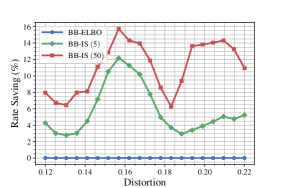
Figure 10: The rate saving curve for lossy compression on the EMNIST-MNIST test set. We measure the net bitrate savings ($\%$) relative to BB-ELBO for fixed distortion values.

6 Conclusion

We showed that extended state space representations of Monte Carlo estimators of the marginal likelihood can be transformed into bits-back schemes that asymptotically remove the $D_{\mathrm{KL}}$ gap. In our toy experiments, our coders were ‘self-cleaning’ in the sense that they reduced the dirty bits gap. In our transfer experiments, our coders had a larger impact on compression rates when compressing out-of-distribution data. Finally, we demonstrated that the initial bit cost incurred by naive variants can be controlled by coupling techniques. We believe these coupling techniques may be of value in other settings to reduce initial bit costs.

Appendix A Monte Carlo Bits-Back Coders

A.1 Notation

• $\mathbb{I}\left(A\right)$ is the indicator function of the event $A$, i.e., $\mathbb{I}\left(A\right)=1$ if $A$ holds and $0$ otherwise.

• ${\mathbb{P}}(A)$ is the probability of the event $A$.

A.2 Assumptions

• We assume that, if $q(z\,|\,x)>0$, then $p(x,z)>0$.

A.3 General Framework

Algorithm 2 Encode Procedure of McBits Coders

Procedure Encode(symbol $x$, message $m$)

       decode $\mathcal{Z}$ with $Q(\mathcal{Z}\,|\,x)$
encode $x$ and $\mathcal{Z}$ with $P(x,\mathcal{Z})$
return $m^{\prime}$

Algorithm 3 Decode Procedure of McBits Coders

Procedure Decode(message $m$)

       decode $x$ and $\mathcal{Z}$ with $P(x,\mathcal{Z})$
encode $\mathcal{Z}$ with $Q(\mathcal{Z}\,|\,x)$
return $x$, $m^{\prime}$

As discussed in the main body, given the extended space representation of an unbiased estimator of the marginal likelihood, we can derive the general procedure of McBits coders as Alg. 2. The decode procedure could be easily derived from the encode procedure by simply reverse the order and switch ‘encode’ with ‘decode’, as in Alg. 3. Therefore, we do not tediously present the decode procedure for each McBits coder in the following subsections.

A.4 Bits-Back Importance Sampling (BB-IS)

Importance sampling (IS) samples $N$ particles $z_{i}\sim q(z_{i}\,|\,x)$ i.i.d. and uses the average importance weight to estimate $p(x)$. The corresponding variational bound (IWAE, Burda et al., 2015) is the log-average importance weight which is given in equation (3). For simplicity, we denote importance weight as $w_{i}=p(x,z_{i})/q(z_{i}\,|\,x)$ and normalized importance weight as $\tilde{w}_{i}=w_{i}/\sum_{i}w_{i}$. The basic importance sampling estimator of $p(x)$ is given by

$$\sum_{i=1}^{N}\frac{w_{i}}{N}=\sum_{i=1}^{N}\frac{1}{N}\frac{p(x,z_{i})}{q(z_{i}\,|\,x)}.$$ (8)

Extended latent space representation

The extended latent space representation of the importance sampling estimator is presented in Alg. 1, from which we can derive the proposal and target distribution as followed:

$$Q(\{z_{i}\}_{i=1}^{N},j\,|\,x)=\tilde{w}_{j}\prod_{i=1}^{N}q(z_{i}\,|\,x)$$ (9)

$$P(x,\{z_{i}\}_{i=1}^{N},j)=\frac{1}{N}p(x,z_{j})\prod_{i\neq j}q(z_{i}\,|\,x).$$ (10)

Now note,

$$\frac{P(x,\{z_{i}\}_{i=1}^{N},j)}{Q(\{z_{i}\}_{i=1}^{N},j\,|\,x)}=\frac{1}{N}\frac{\sum_{i=1}^{N}w_{i}}{w_{j}}\frac{p(x,z_{j})}{q(z_{j}\,|\,x)}=\sum_{i=1}^{N}\frac{w_{i}}{N},$$ (11)

which exactly gives us the IS estimator.

Algorithm 4 Encode Procedure of BB-IS

Procedure Encode(symbol $x$, message $m$)

       decode $\{z_{i}\}_{i=1}^{N}$ with $\prod_{i=1}^{N}q(z_{i}\,|\,x)$
decode $j$ with $\operatorname{Cat}\left(\tilde{w}_{j}\right)$
encode $\{z_{i}\}_{i\neq j}$ with $\prod_{i\neq j}q(z_{i}\,|\,x)$
encode $x$ with $p(x\,|\,z_{j})$
encode $z_{j}$ with $p(z_{j})$
encode $j$ with $\operatorname{Cat}(1/N)$
return $m^{\prime}$

BB-IS Coder

Based on the extended latent space representation, the Bits-Back Importance Sampling (BB-IS) coder is derived in Alg. 4 and visualized in Fig. 4(a). The expected net bit length for encoding a symbol $x$ is:

$$-\operatorname{\mathbb{E}}_{\{z_{i}\}_{i=1}^{N},j}\left[\log\frac{P(x,\{z_{i}\}_{i=1}^{N},j)}{Q(\{z_{i}\}_{i=1}^{N},j\,|\,x)}\right]=-\operatorname{\mathbb{E}}_{\{z_{i}\}_{i=1}^{N}}\left[\log\left(\sum_{i=1}^{N}\frac{w_{i}}{N}\right)\right].$$ (12)

Ignoring the dirty bits issue, i.e., $z_{i}\sim q(z_{i}\,|\,x)$ i.i.d., the expected net bit length exactly achieves the negative IWAE bound.

A.5 Bits-Back Coupled Importance Sampling

The basic idea behind Bits-Back Coupled Importance Sampling is to couple the randomness that generates the particles $z_{i}$. We assume that $q(z\,|\,x)$ has been discretized to precision $r$. In particular, we assume that for all $z\in{\mathbb{S}}^{\prime}$

$$q(z\,|\,x)=\frac{q_{z}}{2^{r}},$$ (13)

where $q_{z}$ is an integer. Note that this assumption is also required for ANS, so this is not an additional assumption. Assume that ${\mathbb{S}}^{\prime}$ is totally ordered (any ordering works) and $u\in\{0\ ..\ 2^{r}-1\}$. Define the unnormalized cumulative distribution function $F_{q}$ of $q$ as well as the following related objects:

$$F_{q}(z) =\sum_{z^{\prime}\leq z}q_{z^{\prime}}$$ (14)

$$F_{q}^{-1}(u) =\arg\min\{z\in{\mathbb{S}}^{\prime}:F_{q}(z)>u\}$$ (15)

$$U(z) =\{u:F_{q}^{-1}(u)=z\}.$$ (16)

Notice that $|U(z)|=q_{z}$. Thus, if $u\sim\operatorname{unif}\{0\ ..\ 2^{r}-1\}$, then

$${\mathbb{P}}\left(F_{q}^{-1}(u)=z\right) ={\mathbb{P}}\left(u\in U(z)\right)$$

$$=\frac{|U(z)|}{2^{r}}$$

$$=\frac{q_{z}}{2^{r}}.$$

Therefore we can reparameterize the sampling process of $z$ as uniform sampling over $\{0\ ..\ 2^{r}-1\}$ followed by the deterministic mapping $F_{q}^{-1}$. This is a classical approach in non-uniform random variate generation, specialized to this discrete setting. This is visualized in Fig. 5.

Coupled importance sampling (CIS) samples the latent variables by coupling their underlying uniforms. Let $T_{i}:\{0\ ..\ 2^{r}-1\}\to\{0\ ..\ 2^{r}-1\}$ be bijective functions. If $u\sim\operatorname{unif}\{0\ ..\ 2^{r}-1\}$, then

$${\mathbb{P}}\left(T_{i}(u)=u^{\prime}\right) ={\mathbb{P}}\left(u=T_{i}^{-1}(u^{\prime})\right)$$

$$=\frac{\mathbb{I}\left(T_{i}^{-1}(u^{\prime})\in\{0\ ..\ 2^{r}-1\}\right)}{2^{r}}$$

$$=\frac{1}{2^{r}}.$$

Thus, if $u\sim\operatorname{unif}\{0\ ..\ 2^{r}-1\}$, then $T_{i}(u)\overset{d}{=}u$ and $F_{q}^{-1}(T_{i}(u))\sim q(z\,|\,x)$. For example, simple bijective operators $T_{i}$ can be defined as applying fixed “sampling shift” $\bar{u}_{i}\in\{0,1,\dots,2^{r}-1\}$ to $u$:

$$T_{i}(u) =(u+\bar{u}_{i})\ \mathrm{mod}\ 2^{r}$$

$$T_{i}^{-1}(u) =(u-\bar{u}_{i})\ \mathrm{mod}\ 2^{r}.$$

For simplicity, we define $T_{1}$ to employ the zero shift $\bar{u}_{1}=0$, i.e., $T_{1}(u)=u$. We now have the definitions that we need to analyze the extended space construction for coupled importance sampling. Let $u_{1}\sim\operatorname{unif}\{0\ ..\ 2^{-}1\}$. As with IS, we denote importance weight as $w_{i}=p(x,F_{q}^{-1}(T_{i}(u_{1})))/q(F_{q}^{-1}(T_{i}(u_{1}))\,|\,x)$ and the normalized importance weight as $\tilde{w}_{i}=w_{i}/\sum_{i}w_{i}$. The coupled importance sampling estimator of $p(x)$ is given

$$\sum_{i=1}^{N}\frac{w_{i}}{N}=\sum_{i=1}^{N}\frac{1}{N}\frac{p(x,F_{q}^{-1}(T_{i}(u_{1})))}{q(F_{q}^{-1}(T_{i}(u_{1}))\,|\,x)}.$$ (17)

Algorithm 5 Extended Latent Space Representation of Coupled Importance Sampling

Process $Q({\mathcal{Z}}\,|\,x)$

       sample $u_{1}\sim\operatorname{unif}\{0,\ldots,2^{r}-1\}$
for $i=1,\dots,N$ do

             assign $u_{i}=T_{i}(u_{1})$
assign $z_{i}=F_{q}^{-1}(u_{i})$

      compute $\tilde{w}_{i}\propto p(x,z_{i})/q(z_{i}\,|\,x)$
sample $j\sim\operatorname{Cat}(\tilde{w}_{i})$
return $\{z_{i}\}_{i=1}^{N},\{u_{i}\}_{i=1}^{N},j$

Process $P(x,{\mathcal{Z}})$

       sample $j\sim\operatorname{Cat}(1/N)$
sample $z_{j}\sim p(z_{j})$
sample $x\sim p(x|z_{j})$
sample $u_{j}\sim\operatorname{unif}\{u:F_{q}^{-1}(u)=z_{j}\}$
for $i\neq j$ do

             assign $u_{i}=T_{i}(T_{j}^{-1}(u_{j}))$
assign $z_{i}=F_{q}^{-1}(u_{i})$

      return $x,\{z_{i}\}_{i=1}^{N},\{u_{i}\}_{i=1}^{N},j$

Extended latent space representation

The extended latent space representations of the coupled importance sampling estimator is presented in Alg. 5. The $Q$ and $P$ processes have the following probability mass functions. For convenience, let ${\mathbb{U}}=\{0\ ..\ 2^{r}-1\}$ and $z_{i}=F_{q}^{-1}(T_{i}(u_{1}))$.

$$Q(\{z_{i}\}_{i=1}^{N},\{u_{i}\}_{i=1}^{N},j\,|\,x) =\frac{\mathbb{I}\left(u_{1}\in{\mathbb{U}}\right)}{2^{r}}\prod_{i=2}^{N}\mathbb{I}\left(T_{i}(u_{1})=u_{i}\right)\prod_{i=1}^{N}\mathbb{I}\left(F_{q}^{-1}(u_{i})=z_{i}\right)\frac{w_{j}}{\sum_{i=1}^{N}w_{i}}$$ (18)

$$P(x,\{z_{i}\}_{i=1}^{N},\{u_{i}\}_{i=1}^{N},j) =\frac{1}{N}p(x,z_{j})\frac{\mathbb{I}\left(u_{j}\in U(z_{j})\right)}{2^{r}q(z_{j}\,|\,x)}\prod_{i\neq j}\mathbb{I}\left(T_{i}\left(T_{j}^{-1}(u_{j})\right)=u_{i}\right)\mathbb{I}\left(F_{q}^{-1}(u_{i})=z_{i}\right),$$ (19)

where we used the fact that $q_{z_{j}}=2^{r}q(z_{j}\,|\,x)=\,|\,U(z_{j})\,|\,$. Because each $T_{i}$ is a bijection, we have that the range of $T_{i}(u_{1})$ is all of ${\mathbb{U}}$, as $u_{1}$ ranges over ${\mathbb{U}}$. Thus,

$$\frac{\mathbb{I}\left(u_{1}\in{\mathbb{U}}\right)}{2^{r}}\prod_{i=2}^{N}\mathbb{I}\left(T_{i}\left(u_{1}\right)=u_{i}\right)=\frac{\mathbb{I}\left(u_{j}\in{\mathbb{U}}\right)}{2^{r}}\prod_{i\neq j}\mathbb{I}\left(T_{i}\left(T_{j}^{-1}(u_{j})\right)=u_{i}\right).$$ (20)

Moreover, for any $(u,z)\in{\mathbb{U}}\times{\mathbb{S}}^{\prime}$,

$$\frac{\mathbb{I}\left(u\in{\mathbb{U}}\right)}{2^{r}}\mathbb{I}\left(F_{q}^{-1}(u)=z\right)=\frac{\mathbb{I}\left(u\in U(z)\right)}{2^{r}}=q(z\,|\,x)\frac{\mathbb{I}\left(u\in U(z)\right)}{2^{r}q(z\,|\,x)}.$$ (21)

Thus,

$$Q(\{z_{i}\}_{i=1}^{N},\{u_{i}\}_{i=1}^{N},j\,|\,x) =\frac{\mathbb{I}\left(u_{1}\in{\mathbb{U}}\right)}{2^{r}}\prod_{i=2}^{N}\mathbb{I}\left(T_{i}(u_{1})=u_{i}\right)\prod_{i=1}^{N}\mathbb{I}\left(F_{q}^{-1}(u_{i})=z_{i}\right)\frac{w_{j}}{\sum_{i=1}^{N}w_{i}}$$ (22)

$$=\frac{\mathbb{I}\left(u_{j}\in{\mathbb{U}}\right)}{2^{r}}\prod_{i\neq j}\mathbb{I}\left(T_{i}(T_{j}^{-1}(u_{j}))=u_{i}\right)\prod_{i=1}^{N}\mathbb{I}\left(F_{q}^{-1}(u_{i})=z_{i}\right)\frac{w_{j}}{\sum_{i=1}^{N}w_{i}}$$ (23)

$$=q(z_{j}\,|\,x)\frac{\mathbb{I}\left(u_{j}\in U(z_{j})\right)}{2^{r}q(z_{j}\,|\,x)}\prod_{i\neq j}\mathbb{I}\left(T_{i}(T_{j}^{-1}(u_{j}))=u_{i}\right)\mathbb{I}\left(F_{q}^{-1}(u_{i})=z_{i}\right)\frac{w_{j}}{\sum_{i=1}^{N}w_{i}}.$$ (24)

From this it directly follows that

$$\frac{P(x,\{z_{i}\}_{i=1}^{N},\{u_{i}\}_{i=1}^{N},j)}{Q(\{z_{i}\}_{i=1}^{N},\{u_{i}\}_{i=1}^{N},j\,|\,x)}=\frac{1}{N}\frac{\sum_{i=1}^{N}w_{i}}{w_{j}}\frac{p(x,z_{j})}{q(z_{j}\,|\,x)}=\sum_{i=1}^{N}\frac{w_{i}}{N}=\sum_{i=1}^{N}\frac{1}{N}\frac{p(x,F_{q}^{-1}(T_{i}(u_{1})))}{q(F_{q}^{-1}(T_{i}(u_{1}))\,|\,x)},$$ (25)

which is exactly the CIS estimator.

Algorithm 6 Encode Procedure of BB-CIS

Procedure Encode(symbol $x$, message $m$)

       decode $u_{1}$ with $\operatorname{unif}\{0,1,\dots,2^{r}-1\}$
assign $u_{i}=T_{i}(u)$ and $z_{i}=F_{q}^{-1}(u_{i})$ for $i\in\{1,\dots,N\}$
decode $j$ with $\operatorname{Cat}\left(\tilde{w}_{j}\right)$
encode $u_{j}$ with $\operatorname{unif}\{u:F_{q}^{-1}(u)=z_{j}\}$
encode $x$ with $p(x\,|\,z_{j})$
encode $z_{j}$ with $p(z_{j})$
encode $j$ with $\operatorname{Cat}(1/N)$
return $m^{\prime}$

BB-CIS coder

Based on the extended latent space representation, the Bits-Back Coupled Importance Sampling (BB-CIS) coder is derived in Alg. 6 and visualized in Fig. 4(b). The expected net bit length for encoding a symbol $x$ is:

$$-\operatorname{\mathbb{E}}_{u_{1},j}\left[\log\frac{P(x,\{z_{i}\}_{i=1}^{N},\{u_{i}\}_{i=1}^{N},j)}{Q(\{z_{i}\}_{i=1}^{N},\{u_{i}\}_{i=1}^{N},j\,|\,x)}\right]=-\operatorname{\mathbb{E}}_{u_{1}}\left[\log\left(\sum_{i=1}^{N}\frac{w_{i}}{N}\right)\right]=-\operatorname{\mathbb{E}}_{u_{1}}\left[\log\left(\sum_{i=1}^{N}\frac{1}{N}\frac{p(x,F_{q}^{-1}(T_{i}(u_{1})))}{q(F_{q}^{-1}(T_{i}(u_{1}))\,|\,x)}\right)\right].$$ (26)

The convergence of BB-CIS’s net bitrate to $-\log p(x)$ will depend on the $T_{i}$. There are many possibilities, but one consideration is that both sender and receiver must share the $T_{i}$ (or a procedure for generating them). Another consideration is that the number of particles should never exceed $2^{r}$, $N\leq 2^{r}$. This is because we can execute numerical integration with a budget of $2^{r}$ particles. Assuming $T_{i}(u)=i$ for $i\in\{0\ ..\ 2^{r}-1\}$:

$$\sum_{i=1}^{N}\frac{1}{N}\frac{p(x,F_{q}^{-1}(T_{i}(u_{1})))}{q(F_{q}^{-1}(T_{i}(u_{1}))\,|\,x)}=\sum_{u=0}^{2^{r}-1}\frac{1}{2^{r}}\frac{p(x,F_{q}^{-1}(u))}{q(F_{q}^{-1}(u)\,|\,x)}=\sum_{z\in{\mathbb{S}}^{\prime}}q(z\,|\,x)\frac{p(x,z)}{q(z\,|\,x)}=p(x).$$ (27)

We briefly mention two possibilities:

1. Let $T_{i}(u)=(u+k_{i})\ \mathrm{mod}\ 2^{r}$ where $k_{i}\sim\operatorname{unif}\{0\ ..\ 2^{r}-1\}$ i.i.d. generated by a pseudorandom number generator where the sender and receiver share the seed. This will enjoy a convergence rate similar to BB-IS, because $\{(u+k_{i})\ \mathrm{mod}\ 2^{r}\}_{i=1}^{N}$ will be i.i.d. uniform on $\{0\ ..\ 2^{r}-1\}$ for $u\sim\operatorname{unif}\{0\ ..\ 2^{r}-1\}$.

2. Inspired by the idea of numerical integration, let $T_{i}(u)=(u+k_{i})\ \mathrm{mod}\ 2^{r}$ where $k_{i}$ is the $i$th element of a random permutation of $\{0\ ..\ 2^{r}-1\}$. With this scheme, BB-CIS is performing numerical integration on a random permutation of $\{0\ ..\ 2^{r}-1\}$. The rate at which the net bitrate converges to $-\log p(x)$ could clearly be made worse by inefficient permutations. Randomizing the order may help avoid such inefficient permutations. We did not experiment with this.

A.6 Bits-Back Annealed Importance Sampling

Annealed importance sampling (AIS) generalizes importance sampling by introducing a path of intermediate distributions between the tractable base distribution $q(z\,|\,x)$ and the unnormalized target distribution $p(x,z)$. For AIS with $N$ steps, for $i\in\{0,\dots,N\}$, define annealing distributions

$$\pi_{i}(z)\propto f_{i}(z)=q(z\,|\,x)^{1-\beta_{i}}p(x,z)^{\beta_{i}}$$ (28)

$$\beta_{i}\in[0,1],\beta_{0}=0,\beta_{i}<\beta_{i+1},\beta_{N}=1.$$ (29)

Note that $\pi_{0}(z)=f_{0}(z)=q(z\,|\,x)$. Then define the MCMC transition operator $\mathcal{T}_{i}$ that leave the intermediate distribution $\pi_{i}$ invariant and its reverse $\tilde{\mathcal{T}}_{i}$:

$$\int\mathcal{T}_{i}(z^{\prime}\,|\,z)\pi_{i}(z)\,dz=\pi_{i}(z^{\prime})$$ (30)

$$\tilde{\mathcal{T}}_{i}(z^{\prime}\,|\,z)=\mathcal{T}_{i}(z\,|\,z^{\prime})\frac{\pi_{i}(z^{\prime})}{\pi_{i}(z)}=\mathcal{T}_{i}(z\,|\,z^{\prime})\frac{f_{i}(z^{\prime})}{f_{i}(z)}.$$ (31)

Note, $\tilde{\mathcal{T}}_{i}$ is a normalized distribution. AIS samples a sequence of latents $\{z_{i}\}_{i=1}^{N}$ from base distribution and the MCMC transition kernels (see the Q process in Alg. 7) and obtains an unbiased estimate of $p(x)$ as the importance weight over the extended space.

$$\hat{p}_{N}(x)=\frac{f_{1}(z_{1})f_{2}(z_{2})\dots f_{N}(z_{N})}{f_{0}(z_{1})f_{1}(z_{2})\dots f_{N-1}(z_{N})}.$$ (32)

The corresponding variational bound is the log importance weight:

$$-\operatorname{\mathbb{E}}_{\{z_{i}\}_{i=1}^{N}}\left[\log\frac{f_{1}(z_{1})f_{2}(z_{2})\dots f_{N}(z_{N})}{f_{0}(z_{1})f_{1}(z_{2})\dots f_{N-1}(z_{N})}\right]\geq-\log p(x).$$ (33)

Algorithm 7 Extended Latent Space Representation of Annealed Importance Sampling

Process $Q(\mathcal{Z}\,|\,x)$

       sample $z_{1}\sim q(z_{1}\,|\,x)=\pi_{0}(z_{1})$
for $i=1,\dots,N-1$ do

             sample $z_{i+1}\sim\mathcal{T}_{i}(z_{i+1}\,|\,z_{i})$

      return $\{z_{i}\}_{i=1}^{N}$

Process $P(x,\mathcal{Z})$

       sample $z_{N}\sim p(z_{N})$
for $i=N-1,\dots,1$ do

            sample $z_{i}\sim\tilde{\mathcal{T}}_{i}(z_{i}\,|\,z_{i+1})$

      sample $x\sim p(x\,|\,z_{N})$
return $x,\{z_{i}\}_{i=1}^{N}$

Extended latent space representation

The extended space representation of AIS is derived in (Neal, 2001), as presented in Alg. 7. The extended latent variables contain all the latents $\{z_{i}\}_{i=1}^{N}$. Briefly, given $x$, the distribution $Q$ first samples $z_{1}$ from the base distribution $q(z_{1}\,|\,x)$ and then sample $\{z_{i}\}_{i=2}^{N}$ sequentially from the transition kernel $\mathcal{T}_{i}(z_{i+1}\,|\,z_{i})$. The distribution $P$ first samples $z_{N}$ from the prior $p(z_{N})$, then samples $\{z_{i}\}_{i=N-1}^{1}$ from the reverse transition kernel $\tilde{\mathcal{T}}_{i}(z_{i}\,|\,z_{i+1})$ in the reverse order, and finally samples $x$ from $p(x\,|\,z_{N})$. The proposal distribution and the target distribution can be derived as followed:

$$Q(\{z_{i}\}_{i=1}^{N}) =q(z_{1}\,|\,x)\mathcal{T}_{1}(z_{2}\,|\,z_{1})\mathcal{T}_{2}(z_{3}\,|\,z_{2})\dots\mathcal{T}_{N-1}(z_{N}\,|\,z_{N-1})$$ (34)

$$=f_{0}(z_{1})\mathcal{T}_{1}(z_{2}\,|\,z_{1})\mathcal{T}_{2}(z_{3}\,|\,z_{2})\dots\mathcal{T}_{N-1}(z_{N}\,|\,z_{N-1})$$ (35)

$$P(x,\{z_{i}\}_{i=1}^{N}) =p(x,z_{N})\tilde{\mathcal{T}}_{N-1}(z_{N-1}\,|\,z_{N})\tilde{\mathcal{T}}_{N-2}(z_{N-2}\,|\,z_{N-1})\dots\tilde{\mathcal{T}}_{1}(z_{1}\,|\,z_{2})$$ (36)

$$=f_{N}(z_{N})\tilde{\mathcal{T}}_{N-1}(z_{N-1}\,|\,z_{N})\tilde{\mathcal{T}}_{N-2}(z_{N-2}\,|\,z_{N-1})\dots\tilde{\mathcal{T}}_{1}(z_{1}\,|\,z_{2}).$$ (37)

Now note

$$\frac{P(x,\{z_{i}\}_{i=1}^{N})}{Q(\{z_{i}\}_{i=1}^{N})} =\frac{f_{N}(z_{N})\tilde{\mathcal{T}}_{N-1}(z_{N-1}|z_{N})\tilde{\mathcal{T}}_{N-2}(z_{N-2}|z_{N-1})\dots\tilde{\mathcal{T}}_{1}(z_{1}|z_{2})}{f_{0}(z_{1})\mathcal{T}_{1}(z_{2}|z_{1})\mathcal{T}_{2}(z_{3}|z_{2})\dots\mathcal{T}_{N-1}(z_{N}|z_{N-1})}$$ (38)

$$=\frac{f_{1}(z_{1})f_{2}(z_{2})\dots f_{N}(z_{N})}{f_{0}(z_{1})f_{1}(z_{2})\dots f_{N-1}(z_{N})},$$ (39)

which exactly gives us the AIS estimator. Note that we have used equation (31) above.

Algorithm 8 Encode Procedure of BB-AIS

Procedure Encode(symbol $x$, message $m$)

       decode $z_{1}$ with $q(z_{1}\,|\,x)=\pi_{0}(z_{1})$
for $i=1,\dots,N-1$ do

             decode $z_{i+1}$ with $\mathcal{T}_{i}(z_{i+1}\,|\,z_{i})$

      encode $x$ with $p(x\,|\,z_{N})$
for $i=1,\dots,N-1$ do

             encode $z_{i}$ with $\tilde{\mathcal{T}}_{i}(z_{i}\,|\,z_{i+1})$

      encode $z_{N}$ with $p(z_{N})$
return $m^{\prime}$

Algorithm 9 Encode Procedure of BB-AIS with BitSwap

Procedure Encode(symbol $x$, message $m$)

       decode $z_{1}$ with $q(z_{1}\,|\,x)=\pi_{0}(z_{1})$
for $i=1,\dots,N-1$ do

             decode $z_{i+1}$ with $\mathcal{T}_{i}(z_{i+1}\,|\,z_{i})$
encode $z_{i}$ with $\tilde{\mathcal{T}}_{i}(z_{i}\,|\,z_{i+1})$

      encode $x$ with $p(x\,|\,z_{N})$
encode $z_{N}$ with $p(z_{N})$
return $m^{\prime}$

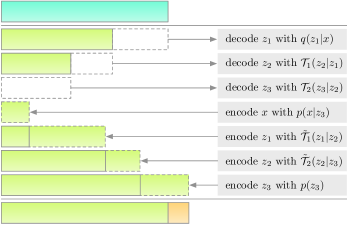
(a) Bits-Back Annealed Importance Sampling

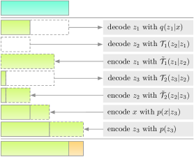
(b) Bits-Back Annealed Importance Sampling with BitSwap

Figure 11: The encoding schemes of BB-AIS and BB-AIS with BitSwap both with $N=3$ steps. Encoding a symbol $x$ with BB-AIS incurs a very large initial bit cost that scales like ${\mathcal{O}}(N)$. This can be significantly reduced by applying the BitSwap trick.

BB-AIS coder

Based on the extended space representation of AIS, the Bits-Back Annealed Importance Sampling coder is derived in Alg. 8 and visualized in Fig. 11(a). The expected net bit length for encoding a symbol $x$ is:

$$-\operatorname{\mathbb{E}}_{\{z_{i}\}_{i=1}^{N}}\left[\frac{\log P(x,\{z_{i}\}_{i=1}^{N})}{\log Q(\{z_{i}\}_{i=1}^{N}\,|\,x)}\right]=-\operatorname{\mathbb{E}}_{\{z_{i}\}_{i=1}^{N}}\left[\log\frac{f_{1}(z_{1})f_{2}(z_{2})\dots f_{N}(z_{N})}{f_{0}(z_{1})f_{1}(z_{2})\dots f_{N-1}(z_{N})}\right].$$ (40)

Ignoring the dirty bits issue, i.e., $\{z_{i}\}_{i=1}^{N}\sim Q(\{z_{i}\}_{i=1}^{N}\,|\,x)$, the expected net bit length exactly achieves the negative AIS bound.

The BB-AIS coder has several practical issues. First is the computational cost. Since the intermediate distributions are usually not factorized over the latent dimensions, it is very inefficient to encode and decode the latents with entropy coders for high dimensional latents. Second is the increased initial bit cost as with BB-IS. More precisely, the initial bits that BB-AIS requires is as followed:

$$-\log q(z_{1}\,|\,x)-\sum_{i=1}^{N-1}\log\mathcal{T}_{i}(z_{i+1}\,|\,z_{i}),$$ (41)

which scales like ${\mathcal{O}}(N)$. However, because the structure of BB-AIS is very similar to the hierarchical latent variable modelss with Markov structure in (Kingma et al., 2019), the BitSwap trick can be applied with BB-AIS to reduce the initial bit cost. The BB-AIS coder with BitSwap is derived in Alg. 9 and visualized in 11(b). In particular, note that the latents $\{z_{i}\}_{i=1}^{N}$ in BB-AIS are encoded and decoded both in the forward time order, we can interleave the encode/decode operations such that $z_{i}$ are encoded with $z_{i+1}$ as soon as $z_{i+1}$ are decoded. Thus there are always at least $-\log\tilde{\mathcal{T}}_{i}(z_{i}\,|\,z_{i+1})$ available for decoding $z_{i+2}$ at the next step, and the initial bit cost is bounded by:

$$-\log q(z_{1}\,|\,x)-\log\mathcal{T}_{1}(z_{2}\,|\,z_{1})+\sum_{i=1}^{N-2}\max(0,-\log\mathcal{T}_{i+1}(z_{i+2}\,|\,z_{i+1})+\log\tilde{\mathcal{T}}_{i}(z_{i}\,|\,z_{i+1})).$$ (42)

Although BitSwap helps to reduce the initial bit cost, we find that it suffers more from the dirty bits issue than the naive implementation and affects the expected net bit length (see Fig. 8(b) for an empirical study). Therefore, using BB-AIS with BitSwap leads to a trade-off between net bitrate distortion and inital bit cost that depends on the number of symbols to be encoded.

A.7 Bits-Back Sequential Monte Carlo

Sequential Monte Carlo (SMC) is a particle filtering method that combines importance sampling with resampling, and its estimate of marginal likelihood typically converges faster than importance sampling for sequential latent variable models (Cérou et al., 2011; Bérard et al., 2014). Suppose the observations are a sequence of $T$ random variables $\bm{x}_{T}\in{\mathbb{S}}^{T}$, where $\bm{x}_{t}:=x_{1:t}$. Sequential latent variable models introduce a sequence of $T$ (unobserved) latent variables $\bm{z}_{T}\in{\mathbb{S}}^{\prime T}$ associated with $\bm{x}_{T}$, where $\bm{z}_{t}:=z_{1:t}$. We assume the joint distribution $p(\bm{x}_{T},\bm{z}_{T})$ can be factored as:

$$p(\bm{x}_{T},\bm{z}_{T})=\prod_{t=1}^{T}f(z_{t}\,|\,\bm{x}_{t-1},\bm{z}_{t-1})g(x_{t}\,|\,\bm{x}_{t-1},\bm{z}_{t}),$$ (43)

where $f$ and $g$ are (generalized) transition and emission distributions, respectively. For the case $t=1$, $f(z_{1}\,|\,\emptyset,\emptyset)=\mu(z_{1})$ reduces to the prior distribution and $g(x_{1}\,|\,\emptyset,z_{1})$ only conditions on $z_{1}$. We also assume the approximate posterior $q(\bm{z}_{T}\,|\,\bm{x}_{T})$ can be factorized as:

$$q(\bm{z}_{T}\,|\,\bm{x}_{T})=\prod_{t=1}^{T}q(z_{t}\,|\,\bm{x}_{t},\bm{z}_{t-1}).$$ (44)

For the case $t=1$, $q(z_{1}\,|\,x_{1},\emptyset)$ only conditions on $x_{1}$.

SMC maintains a population of particle states $\bm{Z}_{t}:=z_{1:t}^{1:N}$. Here we use subscript for indexing timestep $t$ and superscript for indexing particle $i$. In this appendix we describe the version of SMC that resamples at every iteration. Adaptive resampling schemes are possible (Doucet et al., 2001), but we omit them for clarity.

At each time step $t$, each particle independently samples an extension $z_{t}^{i}\sim q(z_{t}^{i}\,|\,\bm{x}_{t},\bm{\tau}_{t-1}^{i})$ where $\bm{\tau}_{t-1}^{i}$ is the ancestral trajectory of the $i$th particle at timestep $t$ (will be described in details later). The sampled extension $z_{t}^{i}$ is appended to $\bm{\tau}_{t-1}^{i}$ to form the trajectory of $i$th particle as $(\bm{\tau}_{t-1}^{i},z_{t}^{i})$. Then the whole population is resampled with probabilities in proportion to importance weights defined as followed:

$$w_{t}^{i}=\frac{f(z_{t}^{i}\,|\,\bm{x}_{t-1},\bm{\tau}_{t-1}^{i})g(x_{t}\,|\,\bm{x}_{t-1},(\bm{\tau}_{t-1}^{i},z_{t}^{i}))}{q(z_{t}^{i}\,|\,\bm{x}_{t},\bm{\tau}_{t-1}^{i})}$$ (45)

$$\tilde{w}_{t}^{i}=\frac{w_{t}^{i}}{\sum_{i=1}^{N}w_{t}^{i}}.$$ (46)

In particular, each particle samples a ‘parent’ index $A_{t}^{i}\sim\operatorname{Cat}(\tilde{w}_{t}^{i})$. At the next timestep $t+1$, the $i$th particle ‘inherits’ the ancestral trajectory of the $A_{t}^{i}$th particle. More precisely,

$$\bm{\tau}_{t}^{i}=(\bm{\tau}_{t-1}^{A_{t}^{i}},z_{t}^{A_{t}^{i}}).$$ (47)

Thus, at timestep $t+1$, given the parent index $A_{t}^{i}$, as well as the collection of particle states $\bm{Z}_{t}$ and previous ancestral indices $\bm{A}_{t-1}:=A_{1:t-1}^{1:N}$, one can trace back the whole ancestral trajectory $\bm{\tau}_{t}^{i}$ by recursively applying equation (47).

For brevity and consistency, we provide the pseudocode (Alg. 10) and visualization (Fig. 12) for tracing back the ancestral trajectory $\bm{\tau}_{t-1}^{i}$ for the $i$th particle at timestep $t$. In particular, we first obtain the ancestral index $B_{k}^{i}$ at each previous timestep $k$ by using the fact

$$B_{k}^{i}=A_{k}^{B_{k+1}^{i}}.$$ (48)

Thus we can obtain a series of ancestral indices $(B_{1}^{i},\dots,B_{t-1}^{i})$ in the backward time order and then obtain the ancestral trajectory by indexing $\bm{Z}_{t-1}$. Note that Alg. 10 is only for helping understand the SMC algorithm, in practice, typically the ancestral trajectories are book-kept and updated along the way using equation (48).

Algorithm 10 Tracing Back the Ancestral Trajectory $\bm{\tau}_{t-1}^{i}$ for the $i$th Particle at Timestep $t$

Procedure TraceBack($\bm{Z}_{t-1},\bm{A}_{t-2}$, $A_{t-1}^{i}$)

       assign $B_{t-1}^{i}=A_{t-1}^{i}$
for $k=t-2,\dots,1$ do

             assign $B_{k}^{i}=A_{k}^{B_{k+1}^{i}}$

      assign $\bm{\tau}_{t-1}^{i}=(z_{1}^{B_{1}^{i}},z_{2}^{B_{2}^{i}},\dots,z_{t-1}^{B_{t-1}^{i}})$
return $\bm{\tau}_{t-1}^{i}$

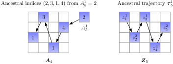
Figure 12: Trace back the ancestral trajectory $\bm{\tau}_{t-1}^{i}$ for the particle $i=1$ at timestep $t=6$.

SMC obtains an unbiased estimate of $p(\bm{x}_{T})$ using the intermediate importance weights (Del Moral, 2004, Proposition 7.4.1):

$$\hat{p}_{N}(\bm{x}_{T})=\prod_{t=1}^{T}\left(\frac{1}{N}\sum_{i=1}^{N}w_{t}^{i}\right).$$ (49)

The corresponding variational bound (FIVO, Maddison et al., 2017; Naesseth et al., 2018; Le et al., 2018) is

$$-\operatorname{\mathbb{E}}_{\bm{Z}_{T},\bm{A}_{T-1}}\left[\sum_{t=1}^{T}\log\left(\frac{1}{N}\sum_{i=1}^{N}w_{t}^{i}\right)\right]\geq-\log p(\bm{x}_{T}).$$ (50)

Algorithm 11 Extended Latent Space Representation of Sequential Monte Carlo

Process $Q(\mathcal{Z}\,|\,\bm{x}_{T})$

       for $t=1,\ldots,T$ do

             if $t\neq 1$ then

                   for $i=1,\ldots,N$ do

                         sample $A^{i}_{t-1}\sim\operatorname{Cat}(\tilde{w}_{t-1})$

                  assign $\bm{A}_{t-1}=\left[\bm{A}_{t-2},A_{t-1}^{1:N}\right]$

            for $i=1,\ldots,N$ do

                   assign $\bm{\tau}_{t-1}^{i}=\mathtt{TraceBack}(\bm{Z}_{t-1},\bm{A}_{t-2},A_{t-1}^{i})$
sample $z_{t}^{i}\sim q(z_{t}^{i}\,|\,\bm{x}_{t},\bm{\tau}_{t-1}^{i})$

            assign $\bm{Z}_{t}=\left[\bm{Z}_{t-1},z_{t}^{1:N}\right]$

      sample $j\sim\operatorname{Cat}(\tilde{w}_{T})$
return $\bm{Z}_{T},\bm{A}_{T-1},j$

 
Process $P(\bm{x}_{T},\mathcal{Z})$

       for $t=1,\ldots,T$ do

             sample $B_{t}\sim\operatorname{Cat}(1/N)$
if $t\neq 1$ then

                   assign $A_{t-1}^{B_{t}}=B_{t-1}$
for $i\neq B_{t}$ do

                         sample $A^{i}_{t-1}\sim\operatorname{Cat}(\tilde{w}_{t-1})$

                  assign $\bm{A}_{t-1}=\left[\bm{A}_{t-2},A_{t-1}^{1:N}\right]$

            assign $\bm{\tau}_{t-1}^{B_{t}}=\mathtt{TraceBack}(\bm{Z}_{t-1},\bm{A}_{t-2},B_{t-1})$
sample $z_{t}^{B_{t}}\sim f(z_{t}^{B_{t}}\,|\,\bm{x}_{t-1},\bm{\tau}_{t-1}^{B_{t}})$
sample $x_{t}\sim g(x_{t}\,|\,\bm{x}_{t-1},(\bm{\tau}_{t-1}^{B_{t}},z_{t}^{B_{t}}))$
for $i\neq B_{t}$ do

                   assign $\bm{\tau}_{t-1}^{i}=\mathtt{TraceBack}(\bm{Z}_{t-1},\bm{A}_{t-2},A^{i}_{t-1})$
sample $z_{t}^{i}\sim q(z_{t}^{i}\,|\,\bm{x}_{t},\bm{\tau}_{t-1}^{i})$

            assign $\bm{Z}_{t}=\left[\bm{Z}_{t-1},z_{t}^{1:N}\right]$

      assign $j=B_{T}$
return $\bm{x}_{T},\bm{Z}_{T},\bm{A}_{T-1},j$

Extended latent space representation

The extended space representation of SMC is derived in (Andrieu et al., 2010), as presented in Alg. 11. The extended latent space variables contain the particle states $\bm{Z}_{T}$, ancestral indices $\bm{A}_{T-1}$, and a particle index $j$ used to pick one special particle trajectory. Briefly, the $Q$ distribution samples $\bm{Z}_{T}$ and $\bm{A}_{T-1}$ in the same manner as SMC, with an additional step that samples the particle index $j$ with probability proportional to the importance weight $w_{T}$. The $P$ distribution selects the ancestral indices of the special particle $(B_{1},\dots,B_{T})$ uniformly, and samples the special particle trajectory $\bm{z}_{T}^{*}=(z_{1}^{B_{1}},\dots,z_{T}^{B_{T}})$ and the observations $\bm{x}_{T}$ jointly with the underlying model distribution. The remaining particle states and ancestral indices are sampled with the same distribution as $Q$. Note that the special particle trajectory $\bm{z}_{T}^{*}=\mathtt{TraceBack}(\bm{Z}_{T},\bm{A}_{T-1},j)$.

From Alg. 11, the proposal distribution and the target distribution and be derived as followed:

$$Q(\bm{Z}_{T},\bm{A}_{T-1},j\,|\,\bm{x}_{T})=\tilde{w}_{T}^{j}\prod_{i=1}^{N}q(z_{1}^{i}|x_{1})\prod_{t=2}^{T}\prod_{i=1}^{N}\tilde{w}_{t-1}^{A^{i}_{t-1}}q(z_{t}^{i}\,|\,\bm{x}_{t},\bm{\tau}_{t-1}^{i})$$ (51)

$$P(\bm{x}_{T},\bm{Z}_{T},\bm{A}_{T-1},j) =\frac{1}{N^{T}}\mu(z_{1}^{B_{1}})g(x_{1}|z_{1}^{B_{1}})\prod_{t=2}^{T}f(z_{t}^{B_{t}}\,|\,\bm{x}_{t-1},\bm{\tau}_{t-1}^{B_{t}})g(x_{t}\,|\,\bm{x}_{t-1},(\bm{\tau}_{t-1}^{B_{t}},z_{t}^{B_{t}}))$$

$$~{}~{}~{}~{}\prod_{i\neq B_{1}}q(z_{1}^{i}|x_{1})\prod_{t=2}^{T}\prod_{i\neq B_{t}}\tilde{w}_{t-1}^{A^{i}_{t-1}}q(z_{t}^{i}\,|\,\bm{x}_{t},\bm{\tau}_{t-1}^{i})$$ (52)

$$=\frac{1}{N^{T}}p(\bm{x}_{T},\bm{z}_{T}^{*})\prod_{i\neq B_{1}}q(z_{1}^{i}|x_{1})\prod_{t=2}^{T}\prod_{i\neq B_{t}}\tilde{w}_{t-1}^{A^{i}_{t-1}}q(z_{t}^{i}\,|\,\bm{x}_{t},\bm{\tau}_{t-1}^{i}).$$ (53)

Now note,

$$\frac{P(\bm{x}_{T},\bm{Z}_{T},\bm{A}_{T-1},j)}{Q(\bm{Z}_{T},\bm{A}_{T-1},j\,|\,\bm{x}_{T})} =\frac{1}{N^{T}\tilde{w}_{T}^{j}}\frac{p(\bm{x}_{T},\bm{z}_{T}^{*})}{q(z_{1}^{B_{1}}|x_{1})\prod_{t=2}^{T}\tilde{w}_{t-1}^{A^{B_{t}}_{t-1}}q(z_{t}^{B_{t}}\,|\,\bm{x}_{t},\bm{\tau}_{t-1}^{B_{t}})}$$ (54)

$$=\frac{1}{N^{T}\tilde{w}_{T}^{j}}\frac{p(\bm{x}_{T},\bm{z}_{T}^{*})}{q(z_{1}^{B_{1}}|x_{1})\prod_{t=2}^{T}\tilde{w}_{t-1}^{B_{t-1}}q(z_{t}^{B_{t}}\,|\,\bm{x}_{t},\bm{\tau}_{t-1}^{B_{t}})}$$ (55)

$$=\frac{1}{N^{T}\prod_{t=1}^{T}\tilde{w}_{t}^{B_{t}}}\frac{\mu(z_{1}^{B_{1}})g(x_{1}|z_{1}^{B_{1}})\prod_{t=2}^{T}f(z_{t}^{B_{t}}\,|\,\bm{x}_{t-1},\bm{\tau}_{t-1}^{B_{t}})g(x_{t}\,|\,\bm{x}_{t-1},(\bm{\tau}_{t-1}^{B_{t}},z_{t}^{B_{t}}))}{q(z_{1}^{B_{1}}|x_{1})\prod_{t=2}^{T}q(z_{t}^{B_{t}}\,|\,\bm{x}_{t},\bm{\tau}_{t-1}^{B_{t}})}$$ (56)

$$=\frac{\prod_{t=1}^{T}w_{t}^{B_{t}}}{N^{T}\prod_{t=1}^{T}\tilde{w}_{t}^{B_{t}}}$$ (57)

$$=\prod_{t=1}^{T}(\frac{1}{N}\sum_{i=1}^{N}w_{t}^{i}),$$ (58)

which exactly gives us the SMC estimator. Note that we have used equation (48) and $B_{T}=j$ in the above derivation.

Algorithm 12 Encode Procedure of BB-SMC

Procedure Encode(symbol $\bm{x}_{T}$, message $m$)

       for $t=1,\ldots,T$ do

             if $t\neq 1$ then

                   for $i=1,\ldots,N$ do

References

- Andrieu et al. (2010) Andrieu, C., Doucet, A., and Holenstein, R. Particle Markov chain Monte Carlo methods. Journal of the Royal Statistical Society: Series B, 72(3):269–342, 2010.
- Ballé et al. (2016) Ballé, J., Laparra, V., and Simoncelli, E. P. End-to-end optimized image compression. arXiv preprint arXiv:1611.01704, 2016.
- Ballé et al. (2018) Ballé, J., Minnen, D., Singh, S., Hwang, S. J., and Johnston, N. Variational image compression with a scale hyperprior. arXiv preprint arXiv:1802.01436, 2018.
- Bérard et al. (2014) Bérard, J., Del Moral, P., and Doucet, A. A lognormal central limit theorem for particle approximations of normalizing constants. Electronic Journal of Probability, 19, 2014.
- Boulanger-Lewandowski et al. (2012) Boulanger-Lewandowski, N., Bengio, Y., and Vincent, P. Modeling temporal dependencies in high-dimensional sequences: Application to polyphonic music generation and transcription. arXiv preprint arXiv:1206.6392, 2012.
- (6) Bradbury, J., Frostig, R., Hawkins, P., Johnson, M. J., Leary, C., Maclaurin, D., and Wanderman-Milne, S. JAX: Composable transformations of Python+NumPy programs.
- Burda et al. (2015) Burda, Y., Grosse, R., and Salakhutdinov, R. Importance weighted autoencoders. arXiv preprint arXiv:1509.00519, 2015.
- Caterini et al. (2018) Caterini, A. L., Doucet, A., and Sejdinovic, D. Hamiltonian variational auto-encoder. In Proceedings of the 32nd International Conference on Neural Information Processing Systems, pp. 8178–8188, 2018.
- Cérou et al. (2011) Cérou, F., Del Moral, P., and Guyader, A. A nonasymptotic theorem for unnormalized Feynman-Kac particle models. In Annales de l’IHP Probabilités et statistiques, volume 47, pp. 629–649, 2011.
- Chung et al. (2015) Chung, J., Kastner, K., Dinh, L., Goel, K., Courville, A. C., and Bengio, Y. A recurrent latent variable model for sequential data. Advances in Neural Information Processing Systems, 28:2980–2988, 2015.
- Cohen et al. (2017) Cohen, G., Afshar, S., Tapson, J., and Van Schaik, A. Emnist: Extending mnist to handwritten letters. In 2017 International Joint Conference on Neural Networks (IJCNN), pp. 2921–2926. IEEE, 2017.
- Cover & Thomas (1991) Cover, T. M. and Thomas, J. A. Elements of Information Theory. Wiley Series in Telecommunications. 1991.
- Cremer et al. (2017) Cremer, C., Morris, Q., and Duvenaud, D. Reinterpreting importance-weighted autoencoders. arXiv preprint arXiv:1704.02916, 2017.
- Del Moral (2004) Del Moral, P. Feynman-Kac Formulae: Genealogical and Interacting Particle Systems with Applications. Springer, 2004.
- Devroye (2006) Devroye, L. Nonuniform random variate generation. Handbooks in operations research and management science, 13:83–121, 2006.
- Dinh et al. (2014) Dinh, L., Krueger, D., and Bengio, Y. Nice: Non-linear independent components estimation. arXiv preprint arXiv:1410.8516, 2014.
- Dinh et al. (2016) Dinh, L., Sohl-Dickstein, J., and Bengio, S. Density estimation using real nvp. arXiv preprint arXiv:1605.08803, 2016.
- Domke & Sheldon (2018) Domke, J. and Sheldon, D. R. Importance weighting and variational inference. In Advances in Neural Information Processing Systems, pp. 4470–4479, 2018.
- Doucet et al. (2001) Doucet, A., De Freitas, N., and Gordon, N. An introduction to sequential Monte Carlo methods. In Sequential Monte Carlo Methods in Practice, pp. 3–14. Springer, 2001.
- Duda (2009) Duda, J. Asymmetric numeral systems. arXiv preprint arXiv:0902.0271, 2009.
- Finke (2015) Finke, A. On extended state-space constructions for Monte Carlo methods. PhD thesis, University of Warwick, 2015.
- Flamich et al. (2020) Flamich, G., Havasi, M., and Hernández-Lobato, J. M. Compressing images by encoding their latent representations with relative entropy coding. In Larochelle, H., Ranzato, M., Hadsell, R., Balcan, M. F., and Lin, H. (eds.), Advances in Neural Information Processing Systems, volume 33, pp. 16131–16141. Curran Associates, Inc., 2020. URL https://proceedings.neurips.cc/paper/2020/file/ba053350fe56ed93e64b3e769062b680-Paper.pdf.
- Frey (1998) Frey, B. J. Graphical Models for Machine Learning and Digital Communications. MIT Press, 1998.
- Frey & Hinton (1997) Frey, B. J. and Hinton, G. E. Efficient stochastic source coding and an application to a Bayesian network source model. The Computer Journal, 40(2_and_3):157–165, 1997.
- Havasi et al. (2019) Havasi, M., Peharz, R., and Hernández-Lobato, J. M. Minimal random code learning: Getting bits back from compressed model parameters. In International Conference on Learning Representations, 2019.
- Higgins et al. (2016) Higgins, I., Matthey, L., Pal, A., Burgess, C., Glorot, X., Botvinick, M., Mohamed, S., and Lerchner, A. beta-vae: Learning basic visual concepts with a constrained variational framework. 2016.
- Hinton & Van Camp (1993) Hinton, G. E. and Van Camp, D. Keeping the neural networks simple by minimizing the description length of the weights. In Proceedings of the sixth annual conference on Computational Learning Theory, pp. 5–13, 1993.
- Hoogeboom et al. (2019) Hoogeboom, E., Peters, J., van den Berg, R., and Welling, M. Integer discrete flows and lossless compression. In Advances in Neural Information Processing Systems, pp. 12134–12144, 2019.
- Jang et al. (2016) Jang, E., Gu, S., and Poole, B. Categorical reparameterization with Gumbel-softmax. arXiv preprint arXiv:1611.01144, 2016.
- Johnston et al. (2019) Johnston, N., Eban, E., Gordon, A., and Ballé, J. Computationally efficient neural image compression. arXiv preprint arXiv:1912.08771, 2019.
- Jordan et al. (1999) Jordan, M. I., Ghahramani, Z., Jaakkola, T. S., and Saul, L. K. An introduction to variational methods for graphical models. Machine learning, 37(2):183–233, 1999.
- Kingma & Welling (2013) Kingma, D. P. and Welling, M. Auto-encoding variational Bayes. arXiv preprint arXiv:1312.6114, 2013.
- Kingma et al. (2019) Kingma, F. H., Abbeel, P., and Ho, J. Bit-swap: Recursive bits-back coding for lossless compression with hierarchical latent variables. arXiv preprint arXiv:1905.06845, 2019.
- Krizhevsky (2009) Krizhevsky, A. Learning multiple layers of features from tiny images. 2009.
- Le et al. (2018) Le, T. A., Igl, M., Rainforth, T., Jin, T., and Wood, F. Auto-encoding sequential Monte Carlo. In International Conference on Learning Representations, 2018.
- MacKay (2003) MacKay, D. J. C. Information Theory, Inference and Learning Algorithms. Cambridge University Press, 2003.
- Maddison et al. (2016) Maddison, C. J., Mnih, A., and Teh, Y. W. The concrete distribution: A continuous relaxation of discrete random variables. arXiv preprint arXiv:1611.00712, 2016.
- Maddison et al. (2017) Maddison, C. J., Lawson, J., Tucker, G., Heess, N., Norouzi, M., Mnih, A., Doucet, A., and Teh, Y. Filtering variational objectives. In Advances in Neural Information Processing Systems, pp. 6573–6583, 2017.
- Minnen et al. (2018) Minnen, D., Ballé, J., and Toderici, G. D. Joint autoregressive and hierarchical priors for learned image compression. In Advances in Neural Information Processing Systems, pp. 10771–10780, 2018.
- Naesseth et al. (2018) Naesseth, C., Linderman, S., Ranganath, R., and Blei, D. Variational sequential Monte Carlo. In Storkey, A. and Perez-Cruz, F. (eds.), Proceedings of the Twenty-First International Conference on Artificial Intelligence and Statistics, volume 84 of Proceedings of Machine Learning Research, pp. 968–977. PMLR, 09–11 Apr 2018. URL http://proceedings.mlr.press/v84/naesseth18a.html.
- Neal (2001) Neal, R. M. Annealed importance sampling. Statistics and Computing, 11(2):125–139, 2001.
- Oord et al. (2017) Oord, A. v. d., Vinyals, O., and Kavukcuoglu, K. Neural discrete representation learning. arXiv preprint arXiv:1711.00937, 2017.
- Radford et al. (2020) Radford, A., Jong Wook, K., Hallacy, C., Ramesh, A., Goh, G., Agarwal, S., Sastry, G., Askell, A., Mishkin, P., Clark, J., Kreuger, G., and Sutskever, I. Learning transferable visual models from natural language supervision, 2020.
- Razavi et al. (2019) Razavi, A., van den Oord, A., and Vinyals, O. Generating diverse high-fidelity images with vq-vae-2. In Advances in Neural Information Processing Systems, pp. 14866–14876, 2019.
- Rezende & Mohamed (2015) Rezende, D. J. and Mohamed, S. Variational inference with normalizing flows. arXiv preprint arXiv:1505.05770, 2015.
- Rezende et al. (2014) Rezende, D. J., Mohamed, S., and Wierstra, D. Stochastic backpropagation and approximate inference in deep generative models. arXiv preprint arXiv:1401.4082, 2014.
- Rippel & Adams (2013) Rippel, O. and Adams, R. P. High-dimensional probability estimation with deep density models. arXiv preprint arXiv:1302.5125, 2013.
- Salakhutdinov & Murray (2008) Salakhutdinov, R. and Murray, I. On the quantitative analysis of deep belief networks. In Proceedings of the 25th International Conference on Machine learning, pp. 872–879, 2008.
- Salimans et al. (2017) Salimans, T., Karpathy, A., Chen, X., and Kingma, D. P. PixelCNN++: Improving the PixelCNN with discretized logistic mixture likelihood and other modifications. In ICLR, 2017.
- Sønderby et al. (2017) Sønderby, C. K., Poole, B., and Mnih, A. Continuous relaxation training of discrete latent variable image models. In Beysian DeepLearning workshop, NIPS, volume 201, 2017.
- Townsend (2020) Townsend, J. A tutorial on the range variant of asymmetric numeral systems, 2020.
- Townsend et al. (2019) Townsend, J., Bird, T., and Barber, D. Practical lossless compression with latent variables using bits back coding. ICLR, 2019.
- Townsend et al. (2020) Townsend, J., Bird, T., Kunze, J., and Barber, D. Hilloc: Lossless image compression with hierarchical latent variable models. ICLR, 2020.
- Vahdat & Kautz (2020) Vahdat, A. and Kautz, J. Nvae: A deep hierarchical variational autoencoder. In NeurIPS, 2020.
- van den Berg et al. (2020) van den Berg, R., Gritsenko, A. A., Dehghani, M., Kaae Sønderby, C., and Salimans, T. Idf++: Analyzing and improving integer discrete flows for lossless compression. arXiv e-prints, pp. arXiv–2006, 2020.
- van den Oord et al. (2016) van den Oord, A., Dieleman, S., Zen, H., Simonyan, K., Vinyals, O., Graves, A., Kalchbrenner, N., Senior, A., and Kavukcuoglu, K. WaveNet: A Generative Model for Raw Audio. arXiv e-prints, art. arXiv:1609.03499, September 2016.
- Walker (1974) Walker, A. J. New fast method for generating discrete random numbers with arbitrary frequency distributions. Electronics Letters, 10(8):127–128, 1974.
- Wallace (1990) Wallace, S., C. Classification by minimum-message-length inference. In Advances in Computing and Information, pp. 72–81, 1990.
- Yang et al. (2020) Yang, Y., Bamler, R., and Mandt, S. Improving inference for neural image compression. arXiv preprint arXiv:2006.04240, 2020.