Energy stable arbitrary order ETD-MS method for gradient flows with Lipschitz nonlinearity

Abstract

We present a methodology to construct efficient high-order in time accurate numerical schemes for a class of gradient flows with appropriate Lipschitz continuous nonlinearity. There are several ingredients to the strategy: the exponential time differencing (ETD), the multi-step (MS) methods, the idea of stabilization, and the technique of interpolation. They are synthesized to develop a generic $k^{th}$ order in time efficient linear numerical scheme with the help of an artificial regularization term of the form $A\tau^{k}\frac{\partial}{\partial t}\mbox{{${\cal L}$}}^{p(k)}u$ where ${\cal L}$ is the positive definite linear part of the flow, $\tau$ is the uniform time step-size. The exponent $p(k)$ is determined explicitly by the strength of the Lipschitz nonlinear term in relation to ${\cal L}$ together with the desired temporal order of accuracy $k$. To validate our theoretical analysis, the thin film epitaxial growth without slope selection model is examined with a fourth-order ETD-MS discretization in time and Fourier pseudo-spectral in space discretization. Our numerical results on convergence and energy stability are in accordance with our theoretical results.

AMS subject classifications: 65M12, 65M70, 65Z05
Key words: Gradient flow, epitaxial thin film growth, exponential time differencing, long time energy stability, arbitrary order scheme, multi-step method.

1 Introduction

Many natural and engineering processes are gradient flows in the sense that the time evolution of the system is in the direction of decreasing certain energy functional associated with the state of the system. They have a wide range of applications in materials science, fluid dynamics [2, 4, 7, 13, 17, 23, 35, 53] as well as in geometry (geometric flows) and PDEs (optimal transportation) [3] among many others. The evolution of these gradient flows could be complicated. Efficient and accurate numerical methods are highly desirable, especially in the generic case of the absence of solution formula. In addition, the evolution process could be long before it settles to certain equilibrium state(s), see for instance [34]. Hence, it is of great importance to design numerical methods that inherits the energy law of the gradient flow, even if in a slightly modified form, if one is interested in the long evolution process such as the coarsening process associated with many phase field models at the large system size regime.

An abundant work exists in the development of (energy) long-time stable schemes and numerical simulation of various gradient flows arising in material science and fluid dynamics using convex splitting, truncation, SAV, and IEQ method among others, see for instance [50, 43, 18, 19, 46, 47, 44, 45, 22], and the references therein. Exponential time differencing (ETD) is a very appealing time discretization method which achieves its high-order accuracy in time with exact treatment of the linear part [5, 15, 16] together with Duhammel’s principle applied to the nonlinear term. The introduction of integrating factor gives rise to a nonlinear integral term. There are two popular approaches in approximating the nonlinear part: Runge-Kutta (RK) method [12, 25, 26] and multi-step(MS) method [26, 27, 24]. Abundant applications of these two methods to various gradient models can be found in [1, 8, 9, 11, 14, 28, 30, 31, 32, 52] . The approximations are usually explicit in order to preserve the efficiency of the ETD method. While it is relatively straightforward to construct numerical schemes of arbitrary order formally via RK or MS method, the energy stability of the algorithms are nontrivial since the explicit treatment of the nonlinear term induces instability, and the existing works involving rigorous energy stability analysis for high accuracy scheme are limited. The authors in [29] proved the energy stability only for the first order ETD scheme for the thin film epitaxial growth model without slope selection (NSS). In a recent work, the idea of stabilization was utilized to develop a second order in time ETD-MS method that is energy stable with the aid of a judiciously chosen stabilizing term of matching order for the NSS equation [8], it’s the first work to provide both the energy stability and convergence results for phase field models theoretically. This idea has been developed further in [9] for a third order in time ETD-MS energy stable scheme for the NSS model, and to even higher orders without detailed proof. Another third-order stabilized energy stable ETD-MS scheme proposed in [11] to approximate the NSS equation also gave a rigorous energy stability analysis, in which a different form of stabilized term $A\tau^{2}\Delta_{N}^{2}(u^{n+1}-u^{n})$ was added with $A=\mathcal{O}(\epsilon^{-2})$ to guarantee energy stability. The purpose of this manuscript is to present a systematic approach to construct ETD-MS based energy stable schemes of arbitrary order in time with the help of an appropriate stabilizing term for a class of gradient flows on a Hilbert space with a positive linear part and a mild nonlinear part satisfying Lipschitz condition in some suitable sense. More importantly, we can make the stabilized coefficient $A$ independent of the small parameter $\epsilon$ or time step-size $\tau$ (i.e., of order $\mathcal{O}(1)$) by a proper choice of $p(k)$ (the spatial order of stabilized term). So far as we know, this is the first result on unconditionally energy stable, arbitrary-order ETD-MS based efficient algorithm for this type of gradient flow.

Let $E(u)$ be a suitable energy functional on a Hilbert space $H$ (with the domain being a subspace of $H$), and let $\frac{\delta E}{\delta u}$ be the variational derivative of $E$ with respect to $u$ in $H$. The associated gradient flow with mobility $M\geq 0$ can then be formulated as follows

$$\frac{\partial u}{\partial t}=-M\frac{\delta E}{\delta u}.$$ (1.1)

Taking inner product with (1.1) and $\frac{\delta E}{\delta u}$ on space $H$ we formally arrive at the following energy equality:

$$\frac{dE(u)}{dt}=-M\left\|\frac{\delta E}{\delta u}\right\|^{2}_{H}\leq 0.$$ (1.2)

This implies that the flow always evolves in the direction of decreasing energy. Notice that both the classical Allen-Cahn model and the Cahn-Hilliard model fall into this framework with the same Ginzburg-Landau free energy but different Hilbert space $H$.

The variational derivative of $E$ can be split into two parts, a linear part $\mbox{{${\cal L}$}}u$, and a nonlinear one $\mbox{{${\cal N}$}}(u)$. In additional, large system size for models arising in material sciences often corresponds the existence of a small parameter in front of the linear term once we non-dimensionalize the system. Formulating the system as an abstract ODE in the Hilbert space $H$ or an ODE system after performing appropriate spatial discretization (say Fourier pseudo-spectral in the spatially periodic case) we have

$$\frac{du}{dt}=-\epsilon\mbox{{${\cal L}$}}u+\mbox{{${\cal N}$}}(u).$$ (1.3)

We will impose the following two assumptions on (1.3) :

1. The operator ${\cal L}$ is non-negative.
   Thus we can define operators $\mbox{{${\cal L}$}}^{\alpha/2}$ for any $\alpha\geq 0$. The domain of operator $\mbox{{${\cal L}$}}^{\alpha/2}$ is denoted by $V^{\alpha}$. For $\alpha=1$ and $\alpha=0$, it is abbreviated as $\mbox{{${\cal D}$}}(\mbox{{${\cal L}$}}^{\frac{1}{2}})=V$ and $\mbox{{${\cal D}$}}(\mbox{{${\cal L}$}}^{0})=H$, respectively;

2. The nonlinear term is Lipschitz continuous in the sense that: $\exists\beta>0,\gamma>0,C_{L}>0$ such that

   $$\left\|\mbox{{${\cal N}$}}(u)-\mbox{{${\cal N}$}}(v)\right\|_{V^{-\beta}}\leq C_{L}\left\|u-v\right\|_{V^{\gamma}},\forall u,v\in V^{\gamma},$$ (1.4)

   where $V^{-\beta}$ is the dual space to $V^{\beta}$ with the duality induced by the inner product on $H$.

The case when ${\cal L}$ is only semi-positive definite or positive definite minus a constant multiply of the identity operator can be treated after we shift the ${\cal L}$ so that it is positive definite, and modify the “nonlinear” term accordingly (now it may contain a linear part).

A typical gradient flow that fits into this abstract framework is the thin film epitaxy growth equation without slope selection (see [21, 40, 34, 36, 37] and references therein):

$$\frac{\partial u}{\partial t}=-\epsilon\Delta^{2}u-\nabla\cdot\left(\frac{\nabla u}{1+|\nabla u|^{2}}\right)$$ (1.5)

with the energy functional given by

$$E(u)=\int_{\Omega}\left(\frac{\epsilon}{2}|\Delta u|^{2}-\frac{1}{2}\ln\left(1+|\nabla u|^{2}\right)\right)\mathrm{d}\mathbf{x},$$ (1.6)

and the Hilbert space $H=L^{2}$, the linear and nonlinear operators are $\mbox{{${\cal L}$}}=\Delta^{2}$, $\mbox{{${\cal N}$}}(u)=-\nabla\cdot\left(\frac{\nabla u}{1+|\nabla u|^{2}}\right)$.

Most gradient flows do not fit into this framework directly. However, many of them enjoy invariant regions in the phase space that attract all solutions such as the Cahn-Hilliard equation, the Allen-Cahn equation and many other reaction-diffusion equations, and the two dimensional Navier-Stokes equations [49] among others. For these models, we could modify the nonlinear term with the help of an appropriate truncation to derive a “prepared” equation as in the theory of inertial manifolds so that certain Lipschitz continuity condition is satisfied [49]. Hence the framework is quite general.

The main contribution of this manuscript is the construction and energy stability analysis of ETD-MS based numerical schemes of arbitrary order for (1.3) under the two assumptions postulated above, with an appropriate stabilization term of the form $A\tau^{k}\frac{d}{dt}\mbox{{${\cal L}$}}^{p(k)}u(t)$ for $k^{th}$ order scheme where $A$ is independent of the small parameter $\epsilon$ or the spatial/temporal discretization. The exponent $p(k)$ is determined explicitly independent of $\epsilon$ or the temporal/spatial grids. These algorithms are highly efficient since only one fixed positive definite constant coefficient elliptic problem needs to be solved at each time step. So far as we know, this is the first time such an efficient systematic approach is presented although it was alluded to in [9].

The rest of the manuscript is organized as follows. We present the numerical scheme together with the energy stability analysis in section 2. Numerical results are presented in section 3. Concluding remarks are offered in section 4.

2 Numerical scheme

In this section, we propose a temporal semi-discrete scheme for (1.3), in which a generic $k^{th}$ order approximation in time is constructed by applying the exponential time differencing and multi-step method. The nonlinear term $\mbox{{${\cal N}$}}(u)$ is treated explicitly and the Lagrange approximation is adopted, leading to a linear system. However, higher order multi-step treatment to nonlinear term gives rise to strong instability, thus to keep the energy decaying property, a $k^{th}$ order regularization term of the form of $A\tau^{k}\frac{d}{dt}\mbox{{${\cal L}$}}^{p(k)}u(t)$ is added with a careful choice of exponent $p(k)$.

2.1 The algorithm

Denote the discrete numerical solution at $t=t^{n}$ by $u^{n}$. The differential form of the numerical scheme for (1.3) is to find $u^{n+1}(t):[t_{n},t_{n+1}]\rightarrow$ an appropriate subspace of $H$ such that

$$\frac{du^{n+1}(t)}{dt}+\epsilon\mbox{{${\cal L}$}}u^{n+1}(t)+A\tau^{k}\frac{d}{dt}\mbox{{${\cal L}$}}^{p(k)}u^{n+1}(t)=\sum_{i=0}^{k-1}\ell_{i}(t-t_{n})\mbox{{${\cal N}$}}(u^{n-i}),$$ (2.1)

where $\ell_{i}(s)$ are the shifted (to the negative range) Lagrange basis polynomial of degree $k$ with the form of

$$\ell_{i}(s)=\prod_{0\leq m\leq k-1\atop m\neq i}\frac{m\tau+s}{(m-i)\tau}=\prod_{0\leq m\leq k-1\atop m\neq i}\frac{m+s/\tau}{m-i}=\sum_{j=0}^{k-1}\xi_{i,j}s^{j},$$ (2.2)

where $\{\xi_{i,j}\}_{j=0}^{k-1}$ are coefficients of the polynomial $\ell_{i}(s)$. Obviously, $\xi_{i,j}\sim\mathcal{O}(\tau^{-j})$. This property will be used later in the stability analysis.

Introducing an integrating factor $e^{\mbox{{${\cal K}$}}t}$ with $\mbox{{${\cal K}$}}=\epsilon\left(I+A\tau^{k}\mbox{{${\cal L}$}}^{p(k)}\right)^{-1}\mbox{{${\cal L}$}}$ and integrating the equation (2.1) from $t^{n}$ to $t^{n+1}$ leads to the following $k^{th}$ order ETD-MS scheme

$$u^{n+1}= e^{-\mbox{{${\cal K}$}}\tau}u^{n}+\sum_{i=0}^{k-1}\int_{0}^{\tau}e^{-\mbox{{${\cal K}$}}(\tau-s)}\ell_{i}(s)ds\,\mbox{{${\cal N}$}}(u^{n-i}).$$ (2.3)

Since the Lagrange interpolation polynomials and the linear operator ${\cal L}$ are known a priori, the algorithm can be simplified. Let $\phi_{j}:=\int_{0}^{\tau}e^{-\mbox{{${\cal K}$}}(\tau-s)}s^{j}ds$ which can be calculated (explicitly) before hand, it can be shown via recurrence formula

$$\left\{\begin{aligned} \phi_{0}=&\mbox{{${\cal K}$}}^{-1}\left(I-e^{-\mbox{{${\cal K}$}}\tau}\right),\\ \phi_{j}=&\mbox{{${\cal K}$}}^{-1}\left(\tau^{j}-j\phi_{j-1}\right),\quad 1\leq j\leq k-1.\end{aligned}\right.$$ (2.4)

Thus the $k^{th}$ order ETD-MS scheme (2.3) can be rewritten as

$$u^{n+1}=e^{-\mbox{{${\cal K}$}}\tau}u^{n}+\sum_{i=0}^{k-1}\sum_{j=0}^{k-1}\xi_{i,j}\phi_{j}\,\mbox{{${\cal N}$}}(u^{n-i}).$$ (2.5)

This is an extremely efficient algorithm, especially since we could pre-calculate the operators involved.

2.2 Energy stability

In this subsection, we establish the energy stability for the scheme (2.1). First we present an interpolation estimation that will be used later.

Lemma 2.1.

For any $u\in V^{\beta}$ and $v\in V^{\gamma}$, $p(k)>\max\{\beta,\gamma\},q\in(0,1)$, and any constants $\hat{C},\tilde{C}$ to be determined for specific problem, the following inequality holds

$$\tau\left\|\frac{du}{dt}\right\|_{V^{\beta}}\left\|\frac{dv}{dt}\right\|_{V^{\gamma}}\leq C_{1}\left\|\frac{du}{dt}\right\|_{H}^{2}+C_{2}\tau^{\frac{2qp(k)}{\beta}}\left\|\frac{du}{dt}\right\|_{V^{p(k)}}^{2}+C_{3}\left\|\frac{dv}{dt}\right\|_{H}^{2}+C_{4}\tau^{\frac{2(1-q)p(k)}{\gamma}}\left\|\frac{dv}{dt}\right\|_{V^{p(k)}}^{2},$$ (2.6)

where

$$C_{1}(\hat{C}) =\frac{1-\beta/p(k)}{2}\hat{C}^{1/(1-\beta/p(k))},\quad C_{2}(\hat{C})=\frac{\beta}{2p(k)}\hat{C}^{-p(k)/\beta},$$ (2.7)

$$C_{3}(\tilde{C}) =\frac{1-\gamma/p(k)}{2}\tilde{C}^{1/(1-\gamma/p(k))},\quad C_{4}(\tilde{C})=\frac{\gamma}{2p(k)}\tilde{C}^{-p(k)/\gamma}.$$

Proof.

Using the interpolation inequality to control $\|\cdot\|_{V^{\beta}}$ by $\|\cdot\|_{H}$ and $\|\cdot\|_{V^{p(k)}}$:

$$\tau\left\|\frac{du}{dt}\right\|_{V^{\beta}}\left\|\frac{dv}{dt}\right\|_{V^{\gamma}}\leq\tau\left\|\frac{du}{dt}\right\|_{H}^{1-\beta/p(k)}\left\|\frac{du}{dt}\right\|_{V^{p(k)}}^{\beta/p(k)}\cdot\left\|\frac{dv}{dt}\right\|_{H}^{1-\gamma/p(k)}\left\|\frac{dv}{dt}\right\|_{V^{p(k)}}^{\gamma/p(k)}.$$ (2.8)

Denote the term in the right hand side (RHS) of (2.8) by $I_{1}$, then we use the Young’s inequality twice to show

$$I_{1}\leq \frac{1}{2}\tau^{2q}\left\|\frac{du}{dt}\right\|_{H}^{2-2\beta/p(k)}\left\|\frac{du}{dt}\right\|_{V^{p(k)}}^{2\beta/p(k)}+\frac{1}{2}\tau^{2-2q}\left\|\frac{dv}{dt}\right\|_{H}^{2-2\gamma/p(k)}\left\|\frac{dv}{dt}\right\|_{V^{p(k)}}^{2\gamma/p(k)}$$

$$\leq \frac{1-\beta/p(k)}{2}\left(\hat{C}\left\|\frac{du}{dt}\right\|_{H}^{2-2\beta/p(k)}\right)^{1/(1-\beta/p(k))}+\frac{\beta}{2p(k)}\left(\frac{\tau^{2q}}{\hat{C}}\left\|\frac{du}{dt}\right\|_{V^{p(k)}}^{2\beta/p(k)}\right)^{p(k)/\beta}$$

$$+\frac{1-\gamma/p(k)}{2}\left(\tilde{C}\left\|\frac{dv}{dt}\right\|_{H}^{2-2\gamma/p(k)}\right)^{1/(1-\gamma/p(k))}+\frac{\gamma}{2p(k)}\left(\frac{\tau^{2-2q}}{\tilde{C}}\left\|\frac{dv}{dt}\right\|_{V^{p(k)}}^{2\gamma/p(k)}\right)^{p(k)/\gamma}$$

$$= C_{1}\left\|\frac{du}{dt}\right\|_{H}^{2}+C_{2}\tau^{\frac{2qp(k)}{\beta}}\left\|\frac{du}{dt}\right\|_{V^{p(k)}}^{2}+C_{3}\left\|\frac{dv}{dt}\right\|_{H}^{2}+C_{4}\tau^{\frac{2(1-q)p(k)}{\gamma}}\left\|\frac{dv}{dt}\right\|_{V^{p(k)}}^{2}.$$ (2.9)

This completes the proof of Lemma 2.1. ∎

Now we come to the energy stability. For simplicity, we denote $\|\cdot\|_{L^{2}(t_{i},t_{j};V^{\alpha})}$ by $\|\cdot\|_{L^{2}(I_{i,j};V^{\alpha})}$ hereafter.

Lemma 2.2.

For system (2.1), the following energy estimation establishes:

$$E(u^{n+1})-E(u^{n})+\left\|\frac{du^{n+1}(t)}{dt}\right\|_{L^{2}(I_{n,n+1};H)}^{2}+A\tau^{k}\left\|\frac{du^{n+1}(t)}{dt}\right\|_{L^{2}(I_{n,n+1};V^{p(k)})}^{2}$$

$$\leq \sum_{j=0}^{k-1}C_{L}\tau^{\frac{1}{2}}\left\|1-\sum_{i=-1}^{j-1}\ell_{i}(t-t_{n})\right\|_{L^{2}(I_{n,n+1})}\left\|\frac{du^{n-j+1}(t)}{dt}\right\|_{L^{2}(I_{n-j,n-j+1};V^{\gamma})}\left\|\frac{du^{n+1}(t)}{dt}\right\|_{L^{2}(I_{n,n+1};V^{\beta})},$$ (2.10)

where the convention $\ell_{-1}(t-t_{n})=0$ has been used.

Proof.

To establish the desired energy estimates, we take inner product of (2.1) with $\frac{du^{n+1}(t)}{dt}$, which gives

$$\left\|\frac{du^{n+1}(t)}{dt}\right\|_{H}^{2}+A\tau^{k}\left\|\frac{du^{n+1}(t)}{dt}\right\|_{V^{p(k)}}^{2}+\frac{d}{dt}E(u^{n+1}(t))$$

$$= \left(\sum_{i=0}^{k-1}\ell_{i}(t-t_{n})\mbox{{${\cal N}$}}(u^{n-i})-\mbox{{${\cal N}$}}(u^{n+1}(t)),\frac{du^{n+1}(t)}{dt}\right)_{H}.$$ (2.11)

Integrating from $t_{n}$ to $t_{n+1}$ gives

$$\left\|\frac{du^{n+1}(t)}{dt}\right\|_{L^{2}(I_{n,n+1};H)}^{2}+A\tau^{k}\left\|\frac{du^{n+1}(t)}{dt}\right\|_{L^{2}(I_{n,n+1};V^{p(k)})}^{2}+E(u^{n+1})-E(u^{n})$$

$$= \int_{t_{n}}^{t_{n+1}}\left(\sum_{i=0}^{k-1}\ell_{i}(t-t_{n})\mbox{{${\cal N}$}}(u^{n-i})-\mbox{{${\cal N}$}}(u^{n+1}(t)),\frac{du^{n+1}(t)}{dt}\right)_{H}dt.$$ (2.12)

Note that the sum of the Lagrange basis functions equals one, i.e., $\sum_{i=0}^{k-1}\ell_{i}(t-t_{n})=1$, thus terms within the integral in RHS of (2.2) (denoted by NLT) can be rewritten as

$$\text{NLT}= \left(\sum_{i=0}^{k-1}\ell_{i}(t-t_{n})　\left(\mbox{{${\cal N}$}}(u^{n-i})-\mbox{{${\cal N}$}}(u^{n+1}(t))\right),\frac{du^{n+1}(t)}{dt}\right)_{H}$$

$$= \left(\sum_{i=0}^{k-1}\ell_{i}(t-t_{n})　\left(\mbox{{${\cal N}$}}(u^{n-i})-\mbox{{${\cal N}$}}(u^{n-i+1})+\cdots+\mbox{{${\cal N}$}}(u^{n})-\mbox{{${\cal N}$}}(u^{n+1}(t))\right),\frac{du^{n+1}(t)}{dt}\right)_{H}$$

$$= \left(\sum_{i=0}^{k-1}\ell_{i}(t-t_{n})　\left(\mbox{{${\cal N}$}}(u^{n})-\mbox{{${\cal N}$}}(u^{n+1}(t))\right),\frac{du^{n+1}(t)}{dt}\right)_{H}$$

$$+\sum_{j=1}^{k-1}\left(\sum_{i=j}^{k-1}\ell_{i}(t-t_{n})　\left(\mbox{{${\cal N}$}}(u^{n-j})-\mbox{{${\cal N}$}}(u^{n-j+1})\right),\frac{du^{n+1}(t)}{dt}\right)_{H}$$

$$= \left(\mbox{{${\cal N}$}}(u^{n})-\mbox{{${\cal N}$}}(u^{n+1}(t)),\frac{du^{n+1}(t)}{dt}\right)_{H}$$

$$+\sum_{j=1}^{k-1}\left(\left(1-\sum_{i=0}^{j-1}\ell_{i}(t-t_{n})\right)　　\left(\mbox{{${\cal N}$}}(u^{n-j})-\mbox{{${\cal N}$}}(u^{n-j+1})\right),\frac{du^{n+1}(t)}{dt}\right)_{H}.$$ (2.13)

Using the Cauchy-Schwartz inequality and the Lipschitz continuity (1.4) makes

$$\int_{t_{n}}^{t_{n+1}}\left(\mbox{{${\cal N}$}}(u^{n})-\mbox{{${\cal N}$}}(u^{n+1}(t)),\frac{du^{n+1}(t)}{dt}\right)_{H}dt$$

$$\leq C_{L}\int_{t_{n}}^{t_{n+1}}\left\|u^{n}-u^{n+1}(t)\right\|_{V^{\gamma}}\left\|\frac{du^{n+1}(t)}{dt}\right\|_{V^{\beta}}dt$$

$$\leq C_{L}\int_{t_{n}}^{t_{n+1}}\tau^{\frac{1}{2}}\left\|\frac{du^{n+1}(t)}{dt}\right\|_{L^{2}(I_{n,n+1};V^{\gamma})}\left\|\frac{du^{n+1}(t)}{dt}\right\|_{V^{\beta}}dt$$

$$\leq C_{L}\tau\left\|\frac{du^{n+1}(t)}{dt}\right\|_{L^{2}(I_{n,n+1};V^{\gamma})}\left\|\frac{du^{n+1}(t)}{dt}\right\|_{L^{2}(I_{n,n+1};V^{\beta})}$$

$$:= \mathrm{NLT_{0}},$$ (2.14)

where the last inequality follows from the Hölder inequality.

Similarly, the remaining terms in RHS of (2.2) can be estimated as

$$\int_{t_{n}}^{t_{n+1}}\left(\left(1-\sum_{i=0}^{j-1}\ell_{i}(t-t_{n})\right)\left(\mbox{{${\cal N}$}}(u^{n-j})-\mbox{{${\cal N}$}}(u^{n-j+1})\right),\frac{du^{n+1}(t)}{dt}\right)_{H}dt$$

$$\leq C_{L}\tau^{\frac{1}{2}}\left\|\frac{du^{n-j+1}(t)}{dt}\right\|_{L^{2}(I_{n-j,n-j+1};V^{\gamma})}\left\|\frac{du^{n+1}(t)}{dt}\right\|_{L^{2}(I_{n,n+1};V^{\beta})}\left\|1-\sum_{i=0}^{j-1}\ell_{i}(t-t_{n})\right\|_{L^{2}(I_{n,n+1})}$$

$$:= \mathrm{NLT_{j}},\quad 1\leq j\leq k-1.$$ (2.15)

This completes the proof. ∎

Next we give an upper bound for the $L^{2}$-integral in time $\left\|1-\sum_{i=0}^{j-1}\ell_{i}(t-t_{n})\right\|_{L^{2}(I_{n,n+1})}$ and further provide the energy stability for scheme (2.1). Recall that in (2.2), the Lagrange basis $\ell_{i}(s)$ is expressed as the polynomial of $s$ with coefficients $\xi_{i,j}$. According to the properties of $\xi_{i,j}$, it’s easy to see

$$\left\|1-\sum_{i=0}^{j-1}\ell_{i}(t-t_{n})\right\|_{L^{2}(I_{n,n+1})}=\left\|1-\sum_{i=0}^{j-1}\sum_{r=0}^{k-1}\xi_{i,r}(t-t_{n})^{r}\right\|_{L^{2}(I_{n,n+1})}=C^{*}_{j}\tau^{1/2},\quad 1\leq j\leq k-1,$$ (2.16)

where the constants $C^{*}_{j}$ are independent of time step-size $\tau$ or the current time $t$. For convenience, we follow the convention of $C_{0}^{*}=1$ hereafter.

We now introduce the following notation for the sake of brevity in presentation.

$$\bm{\overline{C}}_{j}:=\sum_{r=0}^{k-1-j}C_{k-1-r}^{*},\quad j=0,\cdots,k-1.$$ (2.17)

It follows that

$$\bm{\overline{C}}_{j}=\bm{\overline{C}}_{j+1}+C_{j}^{*},\quad\bm{\overline{C}}_{k-1}=C^{*}_{k-1}.$$ (2.18)

Next, we define the following modified energy

$$\tilde{E}(u^{n})= E(u^{n})+C_{L}C_{3}\sum_{j=1}^{k-1}\bm{\overline{C}}_{j}\left\|\frac{du^{n-j+1}(t)}{dt}\right\|_{L^{2}(I_{n-j,n-j+1};H)}^{2}$$

$$+C_{L}C_{4}\sum_{j=1}^{k-1}\bm{\overline{C}}_{j}\tau^{k}\left\|\frac{du^{n-j+1}(t)}{dt}\right\|_{L^{2}(I_{n-j,n-j+1};V^{p(k)})}^{2},$$ (2.19)

where both $C_{3},~{}C_{4}$ depend on $\hat{C}$, $\tilde{C}$ as specified in (2.7).

Thanks to (2.7), $C_{1},C_{3}$ can be made as small as we need so long as we set $\hat{C},\tilde{C}$ small enough. Therefore, for small enough constants $\hat{C}$, $\tilde{C}$ and large enough constant $A$ the following inequalities hold

$$\left(1-C_{L}\left(C_{3}+C_{1}\bm{\overline{C}}_{0}\right)\right)\geq C_{L}C_{3}\bm{\overline{C}}_{1},$$ (2.20)

$$\left(A-C_{L}\left(C_{4}+C_{2}\bm{\overline{C}}_{0}\right)\right)\geq C_{L}C_{4}\bm{\overline{C}}_{1}.$$ (2.21)

Note that $C_{0}^{*}=1$, and hence $\bm{\overline{C}}_{0}=\bm{\overline{C}}_{1}+1$ according to (2.18). Therefore (2.20)–(2.21) are simplified as

$$1 \geq C_{L}\left(C_{3}+C_{1}\right)\bm{\overline{C}}_{0},$$

$$A \geq C_{L}\left(C_{4}+C_{2}\right)\bm{\overline{C}}_{0}.$$

Pick $\hat{C}$ and $\tilde{C}$ so that $C_{L}\left(C_{3}+C_{1}\right)\bm{\overline{C}}_{0}\leq 1$, i.e., $(1-\beta/p(k))\hat{C}^{1/(1-\beta/p(k))}+(1-\gamma/p(k))\tilde{C}^{1/(1-\gamma/p(k))}\leq 2/(C_{L}\bm{\overline{C}}_{0})$, and then let

$$A= C_{L}\left(\frac{\beta}{2p(k)}\hat{C}^{-p(k)/\beta}+\frac{\gamma}{2p(k)}\tilde{C}^{-p(k)/\gamma}\right)\bm{\overline{C}}_{0},$$

we have (2.20)–(2.21).

We are now ready to prove the main result of the energy stability.

Theorem 2.3.

The numerical scheme (2.1) is energy stable in the sense that

$$\tilde{E}(u^{n+1})\leq\tilde{E}(u^{n}),\quad\forall n\geq k,$$ (2.22)

provided that (2.20)–(2.21) are satisfied, and $p(k)=\frac{(\beta+\gamma)k}{2}$.

Proof.

By (2.16), the estimation (2.2) for $\mathrm{NLT_{j}},~{}1\leq j\leq k-1$ can be simplified to

$$\mathrm{NLT_{j}}=C_{L}C_{j}^{*}\tau\left\|\frac{du^{n-j+1}(t)}{dt}\right\|_{L^{2}(I_{n-j,n-j+1};V^{\gamma})}\left\|\frac{du^{n+1}(t)}{dt}\right\|_{L^{2}(I_{n,n+1};V^{\beta})}.$$ (2.23)

Applying Lemma 2.1 to (2.2) and (2.23), these nonlinear terms can be bounded further:

$$\mathrm{NLT_{0}}\leq C_{L}\left[C_{1}\left\|\frac{du^{n+1}(t)}{dt}\right\|_{L^{2}(I_{n,n+1};H)}^{2}+C_{2}\tau^{\frac{2qp(k)}{\beta}}\left\|\frac{du^{n+1}(t)}{dt}\right\|_{L^{2}(I_{n,n+1};V^{p(k)})}^{2}\right.$$

$$\left.+C_{3}\left\|\frac{du^{n+1}(t)}{dt}\right\|_{L^{2}(I_{n,n+1};H)}^{2}+C_{4}\tau^{\frac{2(1-q)p(k)}{\gamma}}\left\|\frac{du^{n+1}(t)}{dt}\right\|_{L^{2}(I_{n,n+1};V^{p(k)})}^{2}\right],$$ (2.24)

$$\mathrm{NLT_{j}}\leq C_{L}C_{j}^{*}\left[C_{1}\left\|\frac{du^{n+1}(t)}{dt}\right\|_{L^{2}(I_{n,n+1};H)}^{2}+C_{2}\tau^{\frac{2qp(k)}{\beta}}\left\|\frac{du^{n+1}(t)}{dt}\right\|_{L^{2}(I_{n,n+1};V^{p(k)})}^{2}\right.$$

$$\left.+C_{3}\left\|\frac{du^{n-j+1}(t)}{dt}\right\|_{L^{2}(I_{n-j,n-j+1};H)}^{2}+C_{4}\tau^{\frac{2(1-q)p(k)}{\gamma}}\left\|\frac{du^{n-j+1}(t)}{dt}\right\|_{L^{2}(I_{n-j,n-j+1};V^{p(k)})}^{2}\right].$$ (2.25)

Choosing indexes $q$ and $p(k)$ to satisfy

$$\frac{2qp(k)}{\beta}=k,\quad\frac{2(1-q)p(k)}{\gamma}=k,$$ (2.26)

and simple calculation shows

$$q=\frac{1}{1+\gamma/\beta},\quad p(k)=\frac{(\beta+\gamma)k}{2}.$$ (2.27)

Then estimates (2.24)–(2.25) give

$$\mathrm{NLT_{0}}\leq C_{L}\left[C_{1}\left\|\frac{du^{n+1}(t)}{dt}\right\|_{L^{2}(I_{n,n+1};H)}^{2}+C_{2}\tau^{k}\left\|\frac{du^{n+1}(t)}{dt}\right\|_{L^{2}(I_{n,n+1};V^{p(k)})}^{2}\right.$$

$$\left.+C_{3}\left\|\frac{du^{n+1}(t)}{dt}\right\|_{L^{2}(I_{n,n+1};H)}^{2}+C_{4}\tau^{k}\left\|\frac{du^{n+1}(t)}{dt}\right\|_{L^{2}(I_{n,n+1};V^{p(k)})}^{2}\right],$$ (2.28)

$$\mathrm{NLT_{j}}\leq C_{L}C_{j}^{*}\left[C_{1}\left\|\frac{du^{n+1}(t)}{dt}\right\|_{L^{2}(I_{n,n+1};H)}^{2}+C_{2}\tau^{k}\left\|\frac{du^{n+1}(t)}{dt}\right\|_{L^{2}(I_{n,n+1};V^{p(k)})}^{2}\right.$$

$$\left.+C_{3}\left\|\frac{du^{n-j+1}(t)}{dt}\right\|_{L^{2}(I_{n-j,n-j+1};H)}^{2}+C_{4}\tau^{k}\left\|\frac{du^{n-j+1}(t)}{dt}\right\|_{L^{2}(I_{n-j,n-j+1};V^{p(k)})}^{2}\right].$$ (2.29)

Unify the expression in (2.24)–(2.25) with the convention of $C_{0}^{*}=1$ and combine (2.28)–(2.29) with (2.2), it yields

$$\left\|\frac{du^{n+1}(t)}{dt}\right\|_{L^{2}(I_{n,n+1};H)}^{2}+A\tau^{k}\left\|\frac{du^{n+1}(t)}{dt}\right\|_{L^{2}(I_{n,n+1};V^{p(k)})}^{2}+E(u^{n+1})-E(u^{n})$$

$$\leq C_{L}\left(C_{3}+C_{1}\sum_{j=0}^{k-1}C_{j}^{*}\right)\left\|\frac{du^{n+1}(t)}{dt}\right\|_{L^{2}(I_{n,n+1};H)}^{2}+C_{L}\left(C_{4}+C_{2}\sum_{j=0}^{k-1}C_{j}^{*}\right)\tau^{k}\left\|\frac{du^{n+1}(t)}{dt}\right\|_{L^{2}(I_{n,n+1};V^{p(k)})}^{2}$$

$$+C_{L}C_{3}\sum_{j=1}^{k-1}C_{j}^{*}\left\|\frac{du^{n-j+1}(t)}{dt}\right\|_{L^{2}(I_{n-j,n-j+1};H)}^{2}+C_{L}C_{4}\tau^{k}\sum_{j=1}^{k-1}C_{j}^{*}\left\|\frac{du^{n-j+1}(t)}{dt}\right\|_{L^{2}(I_{n-j,n-j+1};V^{p(k)})}^{2}.$$ (2.30)

Adding $C_{L}C_{3}\sum_{j=1}^{k-2}\bm{\overline{C}}_{j+1}\left\|\frac{du^{n-j+1}(t)}{dt}\right\|_{L^{2}(I_{n-j,n-j+1};H)}^{2}$, $C_{L}C_{4}\sum_{j=1}^{k-2}\bm{\overline{C}}_{j+1}\tau^{k}\left\|\frac{du^{n-j+1}(t)}{dt}\right\|_{L^{2}(I_{n-j,n-j+1};V^{p(k)})}^{2}$ to both sides of (2.2) and utilizing (2.18), we deduce

$$E(u^{n+1})+\left(1-C_{L}\left(C_{3}+C_{1}\sum_{j=0}^{k-1}C_{j}^{*}\right)\right)\left\|\frac{du^{n+1}(t)}{dt}\right\|_{L^{2}(I_{n,n+1};H)}^{2}$$

$$+\left(A-C_{L}\left(C_{4}+C_{2}\sum_{j=0}^{k-1}C_{j}^{*}\right)\right)\tau^{k}\left\|\frac{du^{n+1}(t)}{dt}\right\|_{L^{2}(I_{n,n+1};V^{p(k)})}^{2}$$

$$+C_{L}C_{3}\sum_{j=1}^{k-2}\bm{\overline{C}}_{j+1}\left\|\frac{du^{n-j+1}(t)}{dt}\right\|_{L^{2}(I_{n-j,n-j+1};H)}^{2}+C_{L}C_{4}\sum_{j=1}^{k-2}\bm{\overline{C}}_{j+1}\tau^{k}\left\|\frac{du^{n-j+1}(t)}{dt}\right\|_{L^{2}(I_{n-j,n-j+1};V^{p(k)})}^{2}$$

$$\leq E(u^{n})+C_{L}C_{3}\bm{\overline{C}}_{1}\left\|\frac{du^{n}(t)}{dt}\right\|_{L^{2}(I_{n-1,n};H)}^{2}+C_{L}C_{4}\bm{\overline{C}}_{1}\tau^{k}\left\|\frac{du^{n}(t)}{dt}\right\|_{L^{2}(I_{n-1,n};V^{p(k)})}^{2}$$

$$+C_{L}C_{3}\sum_{j=2}^{k-1}\bm{\overline{C}}_{j}\left\|\frac{du^{n-j+1}(t)}{dt}\right\|_{L^{2}(I_{n-j,n-j+1};H)}^{2}+C_{L}C_{4}\sum_{j=2}^{k-1}\bm{\overline{C}}_{j}\tau^{k}\left\|\frac{du^{n-j+1}(t)}{dt}\right\|_{L^{2}(I_{n-j,n-j+1};V^{p(k)})}^{2}.$$ (2.31)

Then the modified energy decaying property (2.22) follows from (2.20)–(2.21) and (2.2).

∎

Remark 2.4.

The requirement postulated in (2.20)–(2.21) is sufficient but not necessary. It would be interesting to find the optimal choice of $A$ that guarantees energy stability. Our numerical results presented in the next section suggest that the stability is insensitive to the choice of $A$ for a certain range well below the theoretical requirement that we have derived here. The theoretically optimal $p(k)$ comes from two consideration: (1) it should be as small as possible to avoid large artificial error; (2) it should be large enough to control the nonlinear term when combined with the original dissipation term. The critical $p(k)$ is derived under the condition that we wish to take $A$ to be independent of $\epsilon$. Larger $p(k)$ may lead to larger error, especially for high-frequency solutions. We can use a relatively low-order regularization to reduce the artificial errors, while this treatment may give us an $A$ that depends on $\epsilon$ or $\tau$. In [11], a $A\tau^{2}\left(\Delta^{2}u^{n+1}-\Delta^{2}u^{n}\right)$ regularization term is added in their third-order ETD scheme, the exponent $p(3)=1$ is smaller than our theoretical optimal value, thus the artificial error is supposed to be smaller, while their stabilized coefficient is of order $\mathcal{O}(\epsilon^{-2})$. This is due to the fact that the regularization combined with original dissipation term is insufficient to control the explicit nonlinear term since temporal accuracy of the artificial regularization term has to be kept, thus the surface diffusion term is involved in the energy stability analysis which is of order $\mathcal{O}(\epsilon^{2})$.

Remark 2.5.

Note that the regularization term $A\tau^{k}\frac{\partial}{\partial t}\mbox{{${\cal L}$}}^{p(k)}u$ can be replaced by a Dupont-Douglas type $A\tau^{k-1}\mbox{{${\cal L}$}}^{p(k)}\left(u^{n+1}-u^{n}\right)$ as long as the exact solution is smooth enough. The continuous form adopted here is consistent with the spirit of $ETD$. As we mentioned before, the introduction of high-order regularization may lead to large truncation error for the high-frequency solution, while the convergence in finite time is preserved as we can see in the following numerical tests. For long-time coarsening process with random initial data, two alternative treatment could be considered in the initial evolution until a relatively smooth solution is obtained: 1. use some high-order methods without stabilization; 2. use variable time step-size in the simulation, which is supposed to be very small in the beginning in order to handle the effect of high-frequency components of solution.

3 Numerical example

In this section, we applied the abstract framework to the NSS equation with $k=4$. The two dimensional domain $\Omega=[0,L]^{2}$ with periodic boundary condition is considered. In this case, $\mbox{{${\cal L}$}}=\Delta^{2}$, $\mbox{{${\cal N}$}}(u)=-\nabla\cdot\left(\frac{\nabla u}{1+|\nabla u|^{2}}\right)$ in our general framework. Thus the abstract functional spaces are specified to $H=\{f:f\in L^{2}~{}\text{with zero mean}\}$, $V^{1/2}=\{f:f\in H_{per}^{1}~{}\text{with zero mean}\}$, $V^{\alpha}=\{f:f\in H_{per}^{2\alpha}~{}\text{with zero mean}\}$ and the Lipschitz continuity takes the following form

$$\left\|\mbox{{${\cal N}$}}(u)-\mbox{{${\cal N}$}}(v)\right\|_{V^{-\frac{1}{2}}}\leq\left\|u-v\right\|_{V^{\frac{1}{2}}},$$ (3.1)

that is $\beta=\gamma=\frac{1}{2}$, then equation (2.27) indicates $p(k)=k/2$.

Here we use a fourth-order ETD-MS method to approximate equation (1.5), i.e.,

$$\frac{du^{n+1}(t)}{dt}+\epsilon\Delta^{2}u^{n+1}(t)+A\tau^{4}\frac{d}{dt}\Delta^{4}u^{n+1}(t)=\sum_{i=0}^{3}\ell_{i}(t-t_{n})\mbox{{${\cal N}$}}(u^{n-i}),\quad t\in[t_{n},t_{n+1}].$$ (3.2)

The Lagrange basis functions $\{\ell_{i}(s)\}_{i=0}^{3},~{}0\leq s\leq\tau$ are

$$\ell_{0}(s) =\frac{s^{3}}{6\tau^{3}}+\frac{s^{2}}{\tau^{2}}+\frac{11s}{6\tau}+1,\quad\ell_{1}(s)=-\frac{s^{3}}{2\tau^{3}}-\frac{5s^{2}}{2\tau^{2}}-\frac{3s}{\tau},$$

$$\ell_{2}(s) =\frac{s^{3}}{2\tau^{3}}+\frac{2s^{2}}{\tau^{2}}+\frac{3s}{2\tau},\quad\ell_{3}(s)=-\frac{s^{3}}{6\tau^{3}}-\frac{s^{2}}{2\tau^{2}}-\frac{s}{3\tau}.$$

The corresponding constants in (2.16) are $C_{1}^{*}=\sqrt{9143/3780},\ C_{2}^{*}=\sqrt{157441/7560},\ C_{3}^{*}=\sqrt{212/945}$ and

$$\bm{\overline{C}}_{1}= C_{1}^{*}+C_{2}^{*}+C_{3}^{*}$$

$$= \left(\sqrt{18286}+\sqrt{157441}+\sqrt{1696}\right)/\sqrt{7560}.$$ (3.3)

The constants in (2.6) are $C_{1}=\frac{3}{8}\hat{C}^{4/3},\ C_{2}=\frac{1}{8}\hat{C}^{-4},\ C_{3}=\frac{3}{8}\tilde{C}^{4/3},\ C_{4}=\frac{1}{8}\tilde{C}^{-4}$. Substitute these into (2.20)–(2.21), then we can take $\hat{C}=\tilde{C}=\left(\frac{4}{3(1+\bm{\overline{C}}_{1})}\right)^{3/4}$ to satisfy

$$1-\frac{3\hat{C}^{4/3}}{8}\left(2+\bm{\overline{C}}_{1}\right)\geq\frac{3\hat{C}^{4/3}}{8}\bm{\overline{C}}_{1}.$$

Thus the regularization coefficient $A=\frac{\hat{C}^{-4}}{8}\left(1+\bm{\overline{C}}_{1}\right)=\frac{27\left(1+\bm{\overline{C}}_{1}\right)^{4}}{512}$ with $\bm{\overline{C}}_{1}$ given in (3) is required. However, we will show the numerical results do not depend much on this relatively stringent condition in the following.

Note that initial steps are needed to start the high-order multi-step scheme (3.2) and here we use the ETD-RK method to compute the first three numerical solutions. The general expression of the fourth-order ETD-RK method is illustrated in [33] as

$$\left\{\begin{aligned} a^{n}=&e^{-\epsilon\mbox{{${\cal L}$}}\tau/2}u^{n}+(-\epsilon\mbox{{${\cal L}$}})^{-1}\left(e^{-\epsilon\mbox{{${\cal L}$}}\tau/2}-I\right)\mbox{{${\cal N}$}}(u^{n},t^{n}),\\ b^{n}=&e^{-\epsilon\mbox{{${\cal L}$}}\tau/2}u^{n}+(-\epsilon\mbox{{${\cal L}$}})^{-1}\left(e^{-\epsilon\mbox{{${\cal L}$}}\tau/2}-I\right)\mbox{{${\cal N}$}}(u^{n},t^{n}+\tau/2),\\ c^{n}=&e^{-\epsilon\mbox{{${\cal L}$}}\tau/2}a^{n}+(-\epsilon\mbox{{${\cal L}$}})^{-1}\left(e^{-\epsilon\mbox{{${\cal L}$}}\tau/2}-I\right)\left(2\mbox{{${\cal N}$}}(b^{n},t^{n}+\tau/2)-\mbox{{${\cal N}$}}(u^{n},t^{n})\right),\\ u^{n+1}=&e^{-\epsilon\mbox{{${\cal L}$}}\tau}u^{n}+\tau^{-2}(-\epsilon\mbox{{${\cal L}$}})^{-3}\left\{\left[-4+\epsilon\mbox{{${\cal L}$}}\tau+e^{-\epsilon\mbox{{${\cal L}$}}\tau}\left(4+3\epsilon\mbox{{${\cal L}$}}\tau+(-\epsilon\mbox{{${\cal L}$}}\tau)^{2}\right)\right]\mbox{{${\cal N}$}}\left(u^{n},t^{n}\right)\right.\\ &+2\left[2-\epsilon\mbox{{${\cal L}$}}\tau-e^{-\epsilon\mbox{{${\cal L}$}}\tau}(2+\epsilon\mbox{{${\cal L}$}}\tau)\right]\left(\mbox{{${\cal N}$}}\left(a^{n},t^{n}+\tau/2\right)+\mbox{{${\cal N}$}}\left(b_{n},t_{n}+\tau/2\right)\right)\\ &\left.+\left[-4+3\epsilon\mbox{{${\cal L}$}}\tau-(-\epsilon\mbox{{${\cal L}$}}\tau)^{2}+e^{-\epsilon\mbox{{${\cal L}$}}\tau}(4+\epsilon\mbox{{${\cal L}$}}\tau)\right]\mbox{{${\cal N}$}}\left(c^{n},t^{n}+\tau\right)\right\}.\end{aligned}\right.$$ (3.4)

To solve system (3.2), the spatial discretization is performed by the Fourier pseudo-spectral method with a resolution $N=128$ and this can be efficiently implemented via the fast Fourier transform. The convergence and energy stability tests are provided.

3.1 Temporal convergence test

In this subsection, the fourth order temporal convergence of scheme (3.2) is verified. The parameters are chosen as $L=2\pi$, $\epsilon=0.01$ and terminal time $T=1$. To test the convergence, an artificial forcing term $g$ is added in the right hand side of (3.2) to make the exact solution $u(t)=e^{-t}\cos(2x)\cos(2y)$:

$$g =(-1+64\varepsilon^{2})u-\frac{8u}{1+2e^{-2t}[1-\cos(4x)\cos(4y)]}$$

$$\quad+\frac{16e^{-2t}u}{[1+2e^{-2t}(1-\cos(4x)\cos(4y))]^{2}}[\cos(4x)+\cos(4y)-2\cos(4x)\cos(4y)],$$

and the discrete $L^{2}$ error is calculated. Firstly, the effect of regularized coefficient $A$ on the convergence is examined in Table 1. From which we can see, the errors grow linearly with the increasing of $A$ and the convergence order is preserved for all of the choice of $A$. Then let $A$ be fixed, results for ${p(k)}=1.5$, ${p(k)}=1.9$, ${p(k)}=2.1$ and ${p(k)}=2.5$ are presented in Table 2. While higher order regularization leads to larger error, clear fourth order convergence rates have been observed for all of ${p(k)}$.

Table 1: Temporal convergence of (3.2) with ${p(k)}=2$.

$\tau$	$A=1$		$A=5$		$A=10$		$A=\frac{27\left(1+\bm{\overline{C}}_{1}\right)^{4}}{512}$
	error	order	error	order	error	order	error	order
2.50E-03	6.53e-07		3.26e-06		6.52e-06		1.12e-04
1.25E-03	4.10e-08	3.993	2.05e-07	3.992	4.10e-07	3.991	7.18e-06	3.959
6.25E-04	2.57e-09	3.997	1.28e-08	3.996	2.57e-08	3.996	4.50e-07	3.994
3.13E-04	1.59e-10	4.009	8.04e-10	3.999	1.61e-09	4.000	2.82e-08	3.998
1.56E-04	8.94e-12	4.157	4.96e-11	4.017	9.99e-11	4.007	1.76e-09	4.000

Table 2: Temporal convergence of (3.2) with $A=\frac{27\left(1+\bm{\overline{C}}_{1}\right)^{4}}{512}$.

$\tau$	${p(k)}=1.5$		${p(k)}=1.9$		${p(k)}=2.1$		${p(k)}=2.5$
	error	order	error	order	error	order	error	order
2.50E-03	1.43e-05		6.03e-05		1.34e-04		7.14e-04
1.25E-03	8.99e-07	3.992	3.83e-06	3.976	8.79e-06	3.934	5.29e-05	3.755
6.25E-04	5.63e-08	3.996	2.40e-07	3.995	5.52e-07	3.993	3.56e-06	3.891
3.13E-04	3.52e-09	3.998	1.50e-08	3.998	3.46e-08	3.998	2.25e-07	3.983
1.56E-04	2.19e-10	4.006	9.41e-10	3.998	2.16e-09	4.000	1.41e-08	3.998

3.2 Simulation of coarsening process

In this subsection, the physically interesting coarsening process is simulated. The parameters are now set as $L=12.8$, $\epsilon=0.005$, $T=30000$ and $\tau=10^{-3}$. Two choices for the regularization coefficient $A=\frac{27\left(1+\bm{\overline{C}}_{1}\right)^{4}}{512}$ and $A=10$ are tested. The scaling laws for the energy $E$, average surface roughness $h$ and the average slope $m$ will be shown, that is $E\sim O(-\ln(t))$, $h\sim O(t^{\frac{1}{2}})$ and $m\sim O(t^{\frac{1}{4}})$ as $t\rightarrow\infty$. (See [21, 36, 37] and references therein). The corresponding definitions for these physical quantities are

$$E(u) =\left(-\frac{1}{2}\ln(1+|\nabla u|^{2}),1\right)+\frac{\varepsilon^{2}}{2}\|\Delta u\|^{2},$$

$$h(u,t) =\sqrt{\frac{h^{2}}{|\Omega|}\sum_{x}|u(x,t)-\bar{u}(t)|^{2}},\quad\mbox{with}\quad\bar{u}(t):=\frac{h^{2}}{|\Omega|}\sum_{x}u(x,t),$$

$$m(u,t) =\sqrt{\frac{h^{2}}{|\Omega|}\sum_{x}|\nabla u(\textbf{x}_{i,j},t)|^{2}}.$$

The snapshots of the numerical solution (3.2) at time $t=$ 1, 5000, 10000, 15000, 20000, 30000 with $A=\frac{27\left(1+\bm{\overline{C}}_{1}\right)^{4}}{512}$ and $A=10$ are displayed in Figures 1 and 2 respectively. The evolution of $E$, $h$ and $m$ with two choices of $A$ is established in Figures 3–5, and the linear fitting results for the solution of (3.2) in time interval $[1,400]$ are also presented, which is consistent with the theoretical scaling laws.

Obvious differences of numerical solutions are observed for two choices of $A$ with a uniform step-size $\tau=10^{-3}$, in Figures 1–5. Since random initial data is used, the artificial error arising from high-order regularization term may be large in the initial stage, resulting in the sensitivity to stabilized coefficient $A$. Therefore, an additional coarsening simulation is performed in the following with a variable time step-size, which is set as: $\tau=10^{-6}$ for $t\leq 1$, $\tau=10^{-5}$ for $1<t\leq 10$, $\tau=10^{-4}$ for $10<t\leq 100$ and $\tau=10^{-3}$ for $t>100$ and other parameters are kept. The related results are displayed in Figures 6–7 and Figures 9–11. From which we can see, the sensitivity to $A$ is significantly reduced. Also, minor differences of solutions between two choices of $A$ are observed in Figure 8.

Remark 3.1.

Thanks to the anonymous reviewer for pointing out the differences between snapshots of numerical solution for two choices of $A$ at the same time level, in Figures 1–2. In fact, the introduction of high-order regularization term may result in large truncation error in the beginning since random initial data is chosen, and further lead to different steady phase states. The same simulation of coarsening process is performed with variable time step-sizes and other parameters kept. The time step-size is taken to be small to handle the effect of high-order regularization during the initial evolution of solution and a relatively large step-size is adopted after a smooth solution obtained. With this treatment being taken, the insensitivity to the stabilized coefficient $A$ of our numerical scheme can be observed in Figures 6–11. This exactly shows the necessity of variable step-size in the long-time simulation of coarsening process. The choice of variable step-size is empirical here, and similar idea has been applied in [38, 51]. There are also various adaptive methods regarding to the choice of time step-size, see [10, 20, 42, 54]. In fact, one of our authors, Xiaoming Wang, has already pointed out the feasibility and necessity of using adaptive strategies or hybrid approach (utilize some alternative high-order methods without regularization for the initial stage) for long-time computation in our previous paper [9], and it would be our future work to conduct the adaptive time-stepping strategy with a posterior estimate.

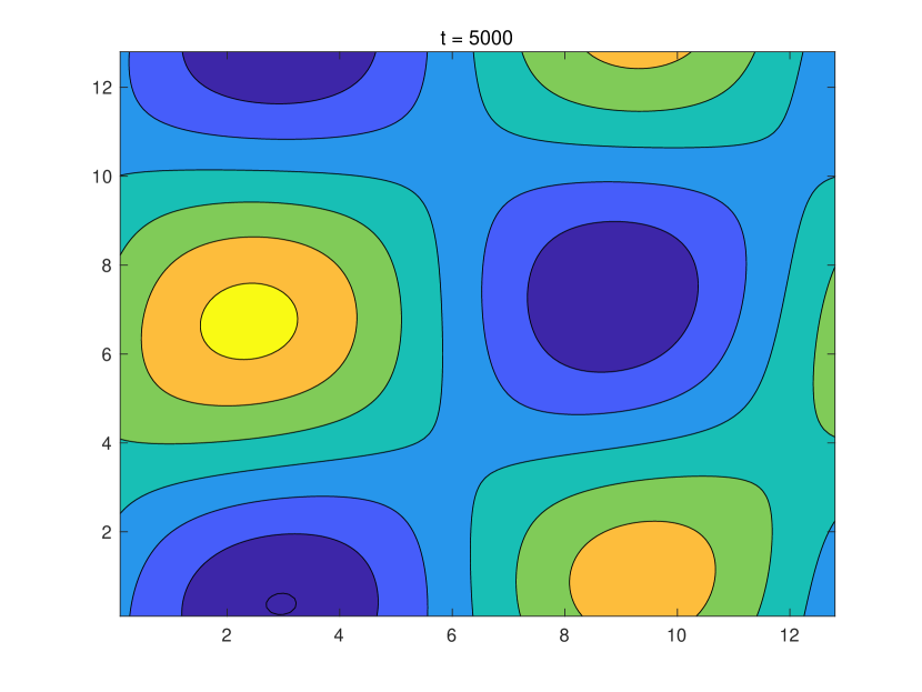
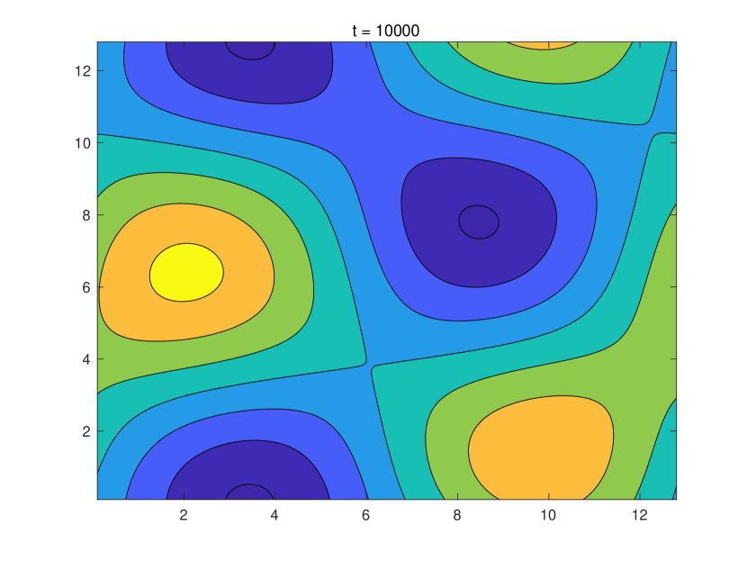
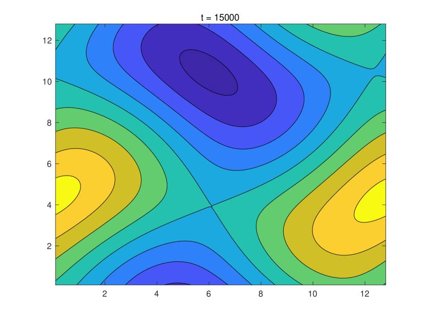
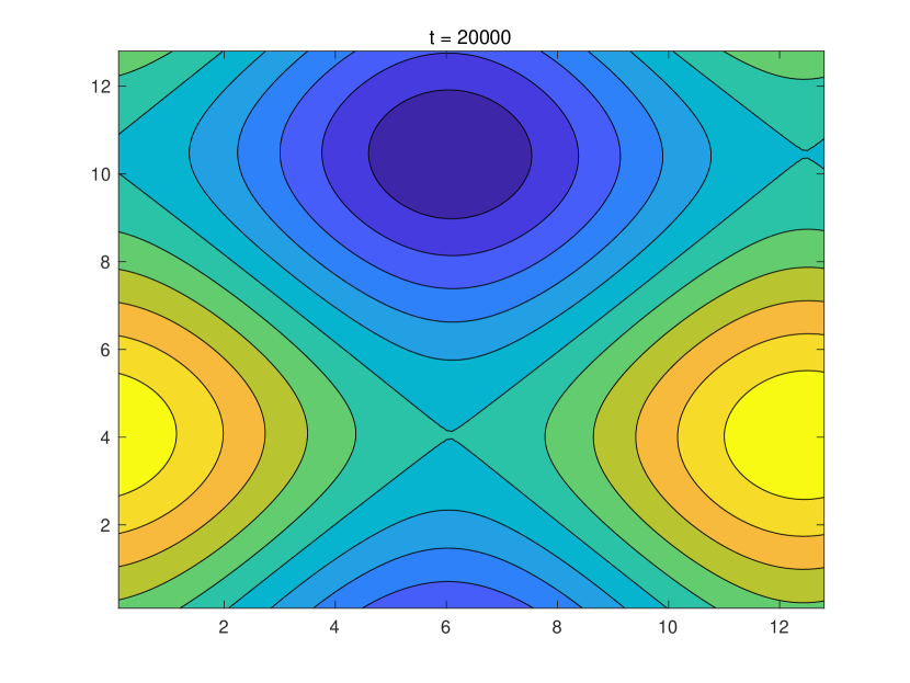
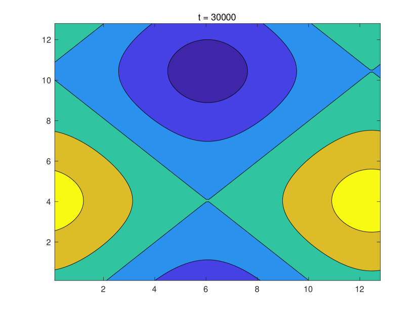
Figure 1: Snapshots of the numerical solutions of scheme (3.2) with $A=\frac{27\left(1+\bm{\overline{C}}_{1}\right)^{4}}{512}$, $\tau=10^{-3}$.

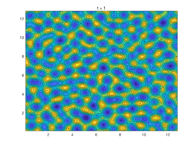
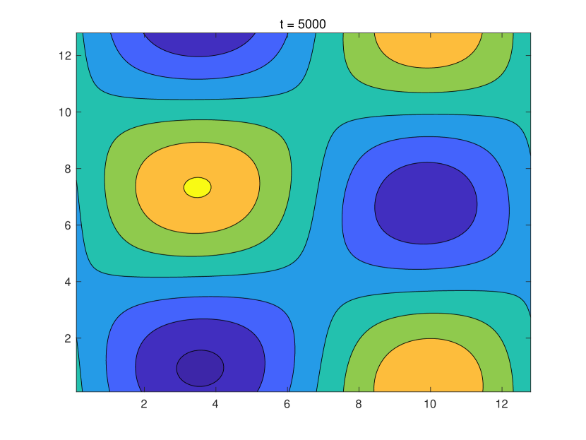
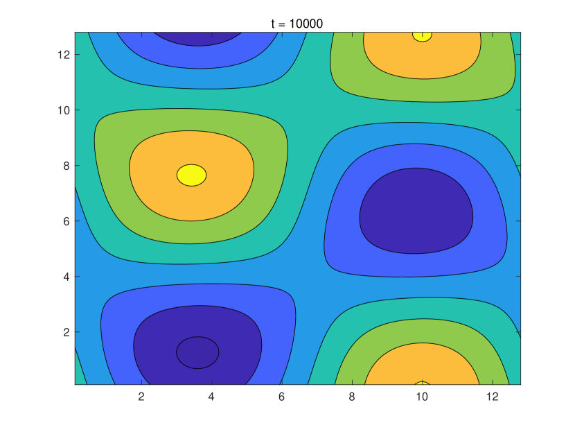
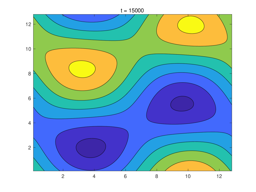
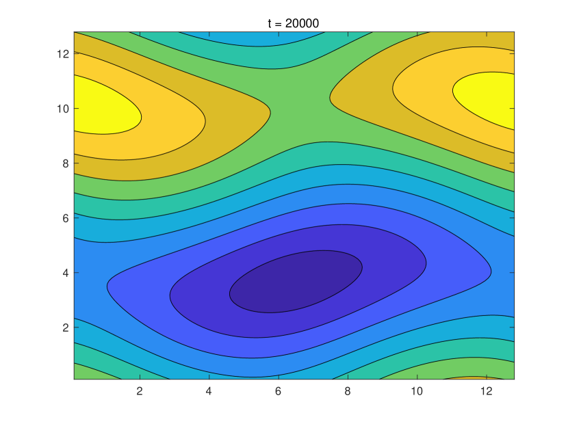
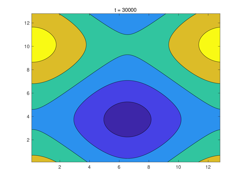
Figure 2: Snapshots of the numerical solutions of scheme (3.2) with $A=10$, $\tau=10^{-3}$.

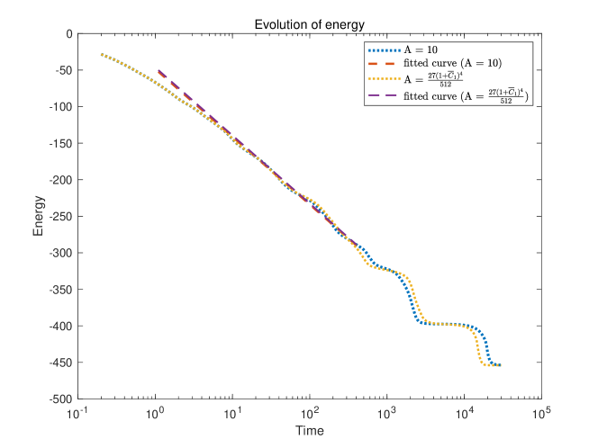
Figure 3: Semi-log plot of the energy $E$ of scheme scheme (3.2) with $\tau=10^{-3}$. Fitted line has the form $a\ln(t)+b$, with coefficients $a=-40.27$, $b=-48.5$ for $A=10$ and $a=-40.45$, $b=-46.35$ for $A=\frac{27\left(1+\bm{\overline{C}}_{1}\right)^{4}}{512}$.

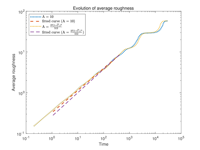
Figure 4: The log-log plot of the average surface roughness $h$ of (3.2) with $\tau=10^{-3}$. Fitted lines have the form $at^{b}$, with coefficients $a=0.3269$, $b=0.5423$ for $A=10$ and $a=0.2657$, $b=0.5771$ for $A=\frac{27\left(1+\bm{\overline{C}}_{1}\right)^{4}}{512}$.

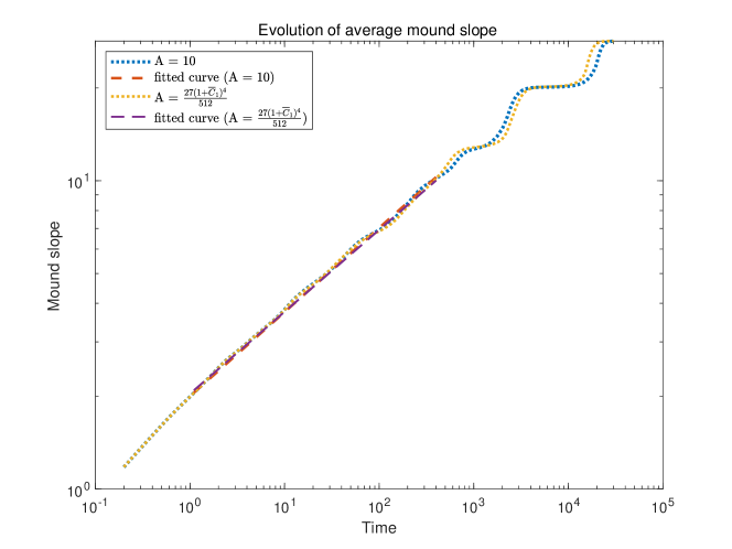
Figure 5: The log-log plot of the average slope $m$ of (3.2) with $\tau=10^{-3}$. Fitted lines have the form $at^{b}$, with coefficients $a=2$, $b=0.2729$ for $A=10$ and $a=2.036$, $b=0.2659$ for $A=\frac{27\left(1+\bm{\overline{C}}_{1}\right)^{4}}{512}$.

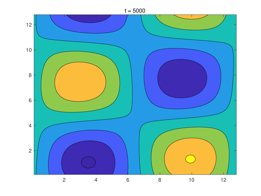
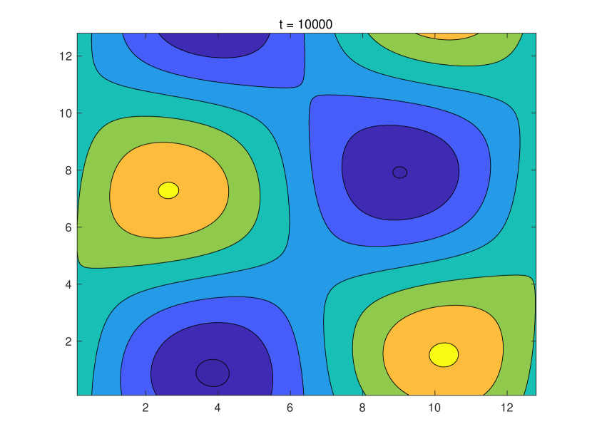
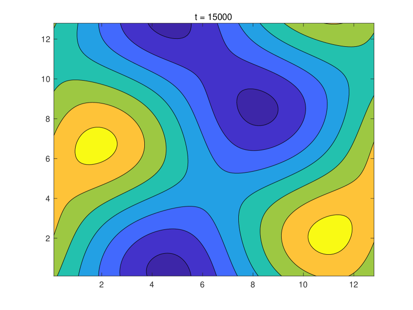
Figure 6: Snapshots of the numerical solutions of scheme (3.2) with $A=\frac{27\left(1+\bm{\overline{C}}_{1}\right)^{4}}{512}$ and variable time step-size: $\tau=10^{-6}$ for $t\leq 1$, $\tau=10^{-5}$ for $1<t\leq 10$, $\tau=10^{-4}$ for $10<t\leq 100$ and $\tau=10^{-3}$ for $t>100$.

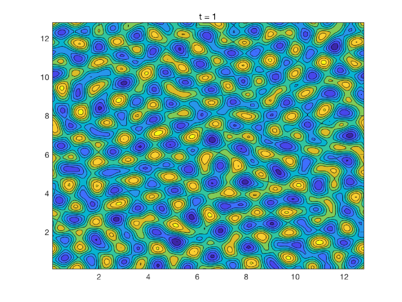
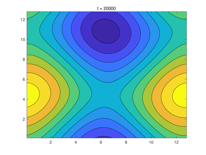
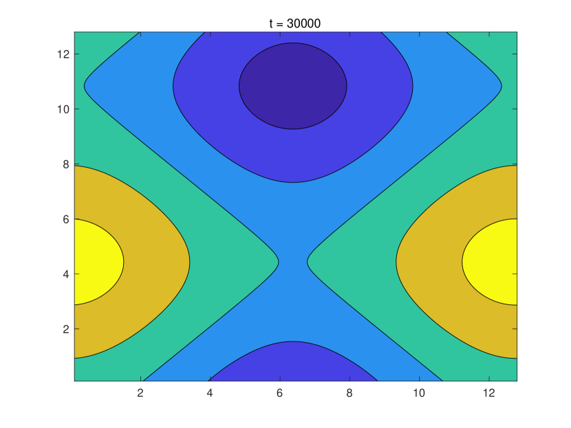
Figure 7: Snapshots of the numerical solutions of scheme (3.2) with $A=10$ and variable time step-size: $\tau=10^{-6}$ for $t\leq 1$, $\tau=10^{-5}$ for $1<t\leq 10$, $\tau=10^{-4}$ for $10<t\leq 100$ and $\tau=10^{-3}$ for $t>100$.

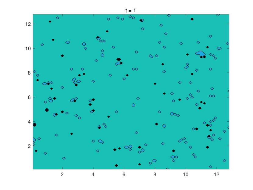
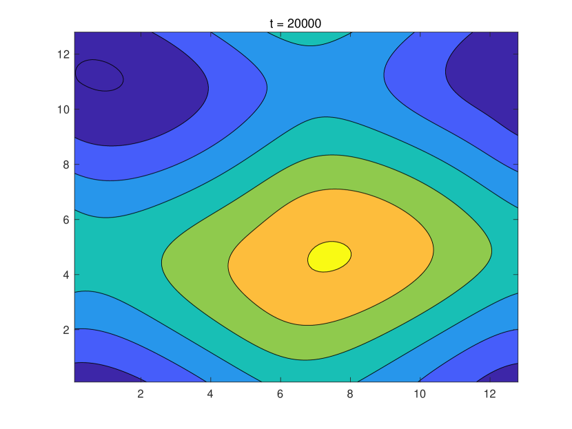
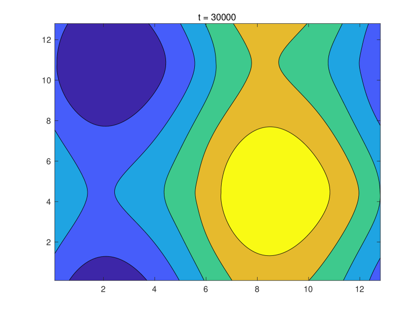
Figure 8: Differences of the numerical solutions of scheme (3.2) between $A=10$ and $A=\frac{27\left(1+\bm{\overline{C}}_{1}\right)^{4}}{512}$ at the same time level for variable time step-size: $\tau=10^{-6}$ for $t\leq 1$, $\tau=10^{-5}$ for $1<t\leq 10$, $\tau=10^{-4}$ for $10<t\leq 100$ and $\tau=10^{-3}$ for $t>100$. The magnitudes of relative difference measured by discrete $L^{2}$-norm in these six snapshots are $10^{-11},~{}10^{-5},~{}10^{-5},~{}10^{-4},~{}10^{-5},~{}10^{-5}$ respectively. The magnitude of numerical solution at time $t=1$ is $1$ and $100$ for the rest.

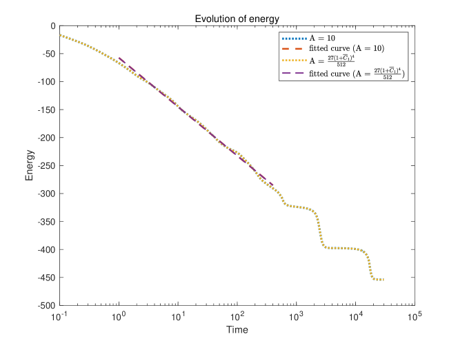
Figure 9: Semi-log plot of the energy $E$ of scheme scheme (3.2) with $\tau=10^{-6}$ for $t\leq 1$, $\tau=10^{-5}$ for $1<t\leq 10$, $\tau=10^{-4}$ for $10<t\leq 100$ and $\tau=10^{-3}$ for $t>100$. Fitted line has the form $a\ln(t)+b$, with coefficients $a=-38.01$, $b=-57.48$ for both $A=10$ and $A=\frac{27\left(1+\bm{\overline{C}}_{1}\right)^{4}}{512}$.

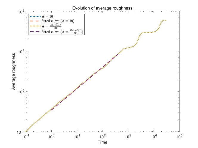
Figure 10: The log-log plot of the average surface roughness $h$ of (3.2) with $\tau=10^{-6}$ for $t\leq 1$, $\tau=10^{-5}$ for $1<t\leq 10$, $\tau=10^{-4}$ for $10<t\leq 100$ and $\tau=10^{-3}$ for $t>100$. Fitted lines have the form $at^{b}$, with coefficients $a=0.3404$, $b=0.5349$ for both $A=10$ and $A=\frac{27\left(1+\bm{\overline{C}}_{1}\right)^{4}}{512}$.

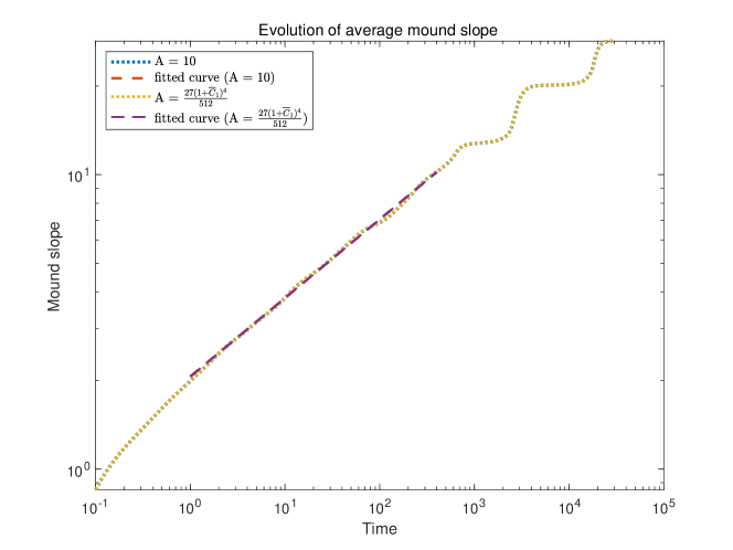
Figure 11: The log-log plot of the average slope $m$ of (3.2) with $\tau=10^{-6}$ for $t\leq 1$, $\tau=10^{-5}$ for $1<t\leq 10$, $\tau=10^{-4}$ for $10<t\leq 100$ and $\tau=10^{-3}$ for $t>100$. Fitted lines have the form $at^{b}$, with coefficients $a=2.062$, $b=0.2669$ for both $A=10$ and $A=\frac{27\left(1+\bm{\overline{C}}_{1}\right)^{4}}{512}$.

4 Conclusions and remarks

A highly efficient $k^{th}$ order accurate and linear numerical scheme is proposed for gradient flows with mild nonlinearity by utilizing ETD and MS methods together with Lagrange interpolation and stabilization. The nonlinear term is treated explicitly and a $k^{th}$ order Dupont-Douglas type regularization $A\tau^{k}\frac{\partial}{\partial t}\mbox{{${\cal L}$}}^{p(k)}u$ is added for stability. The constant $A$ is independent of the small parameter $\epsilon$ or the discretization in space or in time. Lipschitz continuity for the nonlinear term is assumed. The instability caused by the explicit treatment can be totally overcome with the aid of regularization. The exponent $p(k)=\frac{(\beta+\gamma)k}{2}$ is determined explicitly by Lipschitz condition and the order of the scheme. As an example, a fourth order ETD-MS method is applied to a thin film epitaxy model without slope selection, some numerical experiments have been presented to validate the fourth order convergence in time and the unconditional long-time energy stability. The method can be applied to a wide range of gradient flows after proper “preparation” of the original equation.

It is easy to see that our method can be generalized to the case of variable-step without any difficulty. All we need to do is to use a more general Lagrange interpolation polynomial. This opens a door to the development of higher order in time efficient time-adaptive strategies [39]. The Lagrange interpolation polynomials could be replaced by other appropriate interpolations so long as the near decomposition of the identity and the bounded properties are satisfied. The details together with the convergence analysis will be reported in a subsequent work.

References

- [1] E. O. Asante-Asamani, A. Kleefeld, and B. A. Wade. A second-order exponential time differencing scheme for non-linear reaction-diffusion systems with dimensional splitting. Journal of Computational Physics, 109490, 2020.
- [2] S. M. Allen and J. W. Cahn. A microscopic theory for antiphase boundary motion and its application to antiphase domain coarsening. Acta Metallurgica, 27(6):1085–1095, 1979.
- [3] L. Ambrosio and N. Gigli and G. Svare. Gradient Flows in metric spaces and in the space of probability measures, 2nd ed. Birkhauser, 2008.
- [4] D. M. Anderson, G. B. McFadden, and A. A. Wheeler. Diffuse-interface methods in fluid mechanics. Annual Review of Fluid Mechanics, 30(1):139–165, 1998.
- [5] G. Beylkin, J. M. Keiser, and L. Vozovoi. A new class of time discretization schemes for the solution of nonlinear PDEs. Journal of Computational Physics, 147(2):362–387, 1998.
- [6] L. A. Caffarelli and N. E. Muler. An L∞ bound for solutions of the Cahn-Hilliard equation. ArRMA, 133(2):129–144, 1995.
- [7] J. W. Cahn and J. E. Hilliard. Free energy of a nonuniform system. i. interfacial free energy. The Journal of Chemical Physics, 28(2):258–267, 1958.
- [8] W. Chen, W. Li, Z. Luo, C. Wang, and X.Wang. A stabilized second order exponential time differencing multistep method for thin film growth model without slope selection. ESAIM: Mathematical Modelling and Numerical Analysis, 54(3):727–750, 2020.
- [9] W. Chen, W. Li, C. Wang, S. Wang, and X. Wang. Energy stable higher-order linear ETD multi-step methods for gradient flows: application to thin film epitaxy. Special issue dedicated to Professor Andrew Majda on the occasion of his seventieth birthday. Research in the Mathematical Sciences, 7(3):1–27, 2020.
- [10] W. Chen, X. Wang, Y. Yan, and Z. Zhang. A Second Order BDF Numerical Scheme with Variable Steps for the Cahn-Hilliard Equation. SIAM Journal on Numerical Analysis, 57(1):495–525, 2019.
- [11] K. Cheng, Z. Qiao, and C. Wang. A third order exponential time differencing numerical scheme for no-slope-selection epitaxial thin film model with energy stability. Journal of Scientific Computing, 81(1):154–185, 2019.
- [12] S. M. Cox and P. C. Matthews. Exponential time differencing for stiff systems. Journal of Computational Physics, 176(2):430–455, 2002.
- [13] M. Doi and S. F. Edwards. The theory of polymer dynamics, volume 73. Oxford university press, 1988.
- [14] Q. Du, L. Ju, X. Li, and Z. Qiao. Maximum principle preserving exponential time differencing schemes for the nonlocal Allen–Cahn equation. SIAM Journal on Numerical Analysis, 57(2):875–898, 2019.
- [15] Q. Du and W. Zhu. Stability analysis and application of the exponential time differencing schemes. Journal of Computational Mathematics, 200–209, 2004.
- [16] Q. Du and W. Zhu. Analysis and applications of the exponential time differencing schemes and their contour integration modifications. BIT Numerical Mathematics, 45(2):307–328, 2005.
- [17] K. Elder, M. Katakowski, M. Haataja, and M. Grant. Modeling elasticity in crystal growth. Physical Review Letters, 88(24):245701, 2002.
- [18] C. M. Elliott and A. Stuart. The global dynamics of discrete semilinear parabolic equations. SIAM Journal on Numerical Analysis, 30(6):1622–1663, 1993.
- [19] D. J. Eyre. Unconditionally gradient stable time marching the Cahn-Hilliard equation. In Materials Research Society Symposium Proceedings, 529:39–46, 1998.
- [20] X. Feng, T. Tang, and J. Yang. Long time numerical simulations for phase-field problems using p-adaptive spectral deferred correction methods. SIAM Journal on Scientific Computing, 37(1):A271–A294, 2015.
- [21] L. Golubovic. Interfacial coarsening in epitaxial growth models without slope selection. Physical Review Letters, 78(1):90–93, 1997.
- [22] Y. Gong, J. Zhao, and Q. Wang. Arbitrarily high-order unconditionally energy stable sav schemes for gradient flow models. Computer Physics Communications, 249:107033, 2020.
- [23] M. E. Gurtin, D. Polignone, and J. Vinals. Two-phase binary fluids and immiscible fluids described by an order parameter. Mathematical Models and Methods in Applied Sciences, 6(06):815–831, 1996.
- [24] E. Hairer, S. P. Noersett, and G. Wanner. Solving ordinary differential equations i. nonstiff problems. Springer Ser. Comput. Math, 8, 1993.
- [25] M. Hochbruck and A. Ostermann. Explicit exponential Runge-Kutta methods for semilinear parabolic problems. SIAM Journal on Numerical Analysis, 43(3):1069–1090, 2005.
- [26] M. Hochbruck and A. Ostermann. Exponential integrators. Acta Numer., 19(May):209–286, 2010.
- [27] M. Hochbruck and A. Ostermann. Exponential multistep methods of Adams-type. BIT Numerical Mathematics, 51(4):889–908, 2011.
- [28] J. Huang, L. Ju, and B. Wu. A fast compact exponential time differencing method for semilinear parabolic equations with Neumann boundary conditions. Applied Mathematics Letters, 94, 257–265, 2019.
- [29] L. Ju, X. Li, Z. Qiao, and H. Zhang. Energy stability and error estimates of exponential time differencing schemes for the epitaxial growth model without slope selection. Mathematics of Computation, 87(312):1859–1885, 2018.
- [30] L. Ju, X. Liu, and W. Leng. Compact implicit integration factor methods for a family of semilinear fourth-order parabolic equations. Discrete & Continuous Dynamical Systems-B, 19(6):1667–1687, 2014.
- [31] L. Ju, J. Zhang, and Q. Du. Fast and accurate algorithms for simulating coarsening dynamics of Cahn-Hilliard equations. Computational Materials Science, 108:272–282, 2015.
- [32] L. Ju, J. Zhang, L. Zhu, and Q. Du. Fast explicit integration factor methods for semilinear parabolic equations. Journal of Scientific Computing, 62(2): 431–455, 2015.
- [33] A. Kassam and L. N. Trefethen. Fourth-order time-stepping for stiff PDEs. SIAM Journal on Scientific Computing, 26(4):1214–1233, 2005.
- [34] R. V. Kohn and X. Yan. Upper bound on the coarsening rate for an epitaxial growth model. Communications on Pure and Applied Mathematics: A Journal Issued by the Courant Institute of Mathematical Sciences, 56(11):1549–1564, 2003.
- [35] F. M. Leslie. Theory of flow phenomena in liquid crystals. Advances in liquid crystals, 4:1–81, 1979.
- [36] B. Li and J. Liu. Thin film epitaxy with or without slope selection. European Journal of Applied Mathematics, 14(6):713–743, 2003.
- [37] B. Li and J. Liu. Epitaxial growth without slope selection: Energetics, coarsening, and dynamic scaling. Journal of Nonlinear Science, 14(5):429–451, 2004.
- [38] W. Li, W. Chen, C. Wang, Y. Yan, and R. He. A second order energy stable linear scheme for a thin film model without slope selection. Journal of Scientific Computing, 76(3): 1905–1937, 2018.
- [39] F. Lou, T. Tang and H. Xie. Parameter-free time adaptivity based on energy evolution for the Cahn-Hilliard equation. Communications in Computational Physics, 19(5):1542–1563, 2016.
- [40] D. Moldovan and L. Golubovic. Interfacial coarsening dynamics in epitaxial growth with slope selection. Physical Review E, 61(6):6190, 2000.
- [41] Y. Morita and K. Tachibana. An entire solution to the Lotka-Volterra competition-diffusion equations. SIAM Journal on Mathematical Analysis, 40(6):2217–2240, 2009.
- [42] Z. Qiao, Z. Zhang, and T. Tang. An adaptive time-stepping strategy for the molecular beam epitaxy models. SIAM Journal on Scientific Computing, 33(3):1395–1414, 2011.
- [43] J. Shen, C. Wang, X. Wang, and S. M. Wise. Second-order convex splitting schemes for gradient flows with Ehrlich-Schwoebel type energy: application to thin film epitaxy. SIAM Journal on Numerical Analysis, 50(1):105-125, 2012.
- [44] J. Shen, J. Xu, and J. Yang. The scalar auxiliary variable (SAV) approach for gradient flows. Journal of Computational Physics, 353:407–416, 2018.
- [45] J. Shen, J. Xu, and J. Yang. A new class of efficient and robust energy stable schemes for gradient flows. SIAM Review, 61(3):474–506, 2019.
- [46] J. Shen and X. Yang. Numerical approximations of Allen-Cahn and Cahn-Hilliard equations. Discrete & Continuous Dynamical Systems-A, 28(4):1669, 2010.
- [47] J. Shin, H. G. Lee, and J. Y. Lee. Unconditionally stable methods for gradient flow using convex splitting Runge-Kutta scheme. Journal of Computational Physics, 347:367–381, 2017.
- [48] Y. Takeuchi. Global dynamical properties of Lotka-Volterra systems. World Scientific, 1996.
- [49] R. Temam. Infinite-dimensional dynamical systems in mechanics and physics, volume 68. Springer Science & Business Media, 1997.
- [50] C. Wang, X. Wang, and S. M. Wise. Unconditionally stable schemes for equations of thin film epitaxy. Discrete & Continuous Dynamical Systems-A, 28(1):405, 2010.
- [51] S. Wang, W. Chen, H. Pan, and C. Wang. Optimal rate convergence analysis of a second order scheme for a thin film model with slope selection. Journal of Computational and Applied Mathematics, 377(15):112855, 2020.
- [52] X. Wang, L. Ju, and Q. Du. Efficient and stable exponential time differencing Runge-Kutta methods for phase field elastic bending energy models. Journal of Computational Physics, 316:21–38, 2016.
- [53] P. Yue, J. J. Feng, C. Liu, and J. Shen. A diffuse-interface method for simulating two-phase flows of complex fluids. Journal of Fluid Mechanics, 515:293, 2004.
- [54] Z. Zhang and Z. Qiao. An adaptive time-stepping strategy for the Cahn-Hilliard equation. Communications in Computational Physics, 11(4):1261–1278, 2012.