Anisotropic cosmological models in Horndeski gravity

Abstract

It was found recently that the anisotropies in the homogeneous Bianchi I cosmology considered within the context of a specific Horndeski theory are damped near the initial singularity instead of being amplified. In this work we extend the analysis of this phenomenon to cover the whole of the Horndeski family. We find that the phenomenon is absent in the K-essence and/or Kinetic Gravity Braiding theories, where the anisotropies grow as one approaches the singularity. The anisotropies are damped at early times only in more general Horndeski models whose Lagrangian includes terms quadratic and cubic in second derivatives of the scalar field. Such theories are often considered as being inconsistent with the observations because they predict a non-constant speed of gravitational waves. However, the predicted value of the speed at present can be close to the speed of light with any required precision, hence the theories actually agree with the present time observations. We consider two different examples of such theories, both characterized by a late self-acceleration and an early inflation driven by the non-minimal coupling. Their anisotropies are maximal at intermediate times and approach zero at early and late times. The early inflationary stage exhibits an instability with respect to inhomogeneous perturbations, suggesting that the initial state of the universe should be inhomogeneous. However, more general Horndeski models may probably be stable.

I Introduction

It is usually assumed that the state of the universe close to the initial singularity should be strongly anisotropic [1, 2, 3]. This belief is based on the fact that spatial anisotropies produce in the Einstein equations terms which become dominant when one goes backwards in time. In other words, anisotropic perturbations grow to the past. When the universe expands, the anisotropy terms decrease faster than the contribution of other forms of energy subject to the dominant energy condition, and the universe rapidly approaches a locally isotropic state during inflation [4], [5] (without the inflationary stage this process may require a longtime or may not happen at all due to the possibility of recollapse). Therefore, thinking about the early history of the universe, one could expect the isotropic phase of inflation to be generically preceded by an anisotropic phase.

Although this argument seems quite robust, an explicit example in which the anisotropies in the Bianchi I homogeneous model are damped at early times instead of being amplified was recently found [6] within the context of a specific Horndeski theory for a gravitating scalar field [7]. Therefore, the initial stage of the universe in this theory is not anisotropic.

It remained unclear whether the finding of [6] is generic or specific only for one particular Horndeski model. To find the answer, we extend in what follows the analysis of [6] to cover the whole of the Horndeski family. We find that the effect of the anisotropy damping is not necessarily present in all Horndeski theories. In particular, it is absent in the the K-essence and/or Kinetic Gravity Braiding theories. The spatial anisotropies in such theories always grow as one approaches the singularity. However, the anisotropies are damped at early (and late) times in more general Horndeski models whose Lagrangian includes terms quadratic and cubic in second derivatives of the scalar field. Such theories are often considered as being inconsistent with the observations because they predict a non-constant speed of gravitational waves (GW) [8, 9, 10], whereas the GW170817 event shows that the GW speed is equal to the speed of light with very high precision [11]. However, the theories actually predict the value of the GW speed at present to be close to unity within the required precision. In addition, the theories admit stable in the future self-accelerating cosmologies. Therefore, they can perfectly agree with the current observations, and we can extrapolate them to the early times as well since no observational data about the GW speed at redshifts $z>0.3$ are currently available.

We consider two different examples of such theories, both characterized by a late time self-acceleration and also by an early time inflation driven by the nonminimal couplings arising in the Horndeski theory. Sometimes this phase is called “kinetic inflation” [12]. The anisotropies in these theories show a maximum at intermediate times and approach zero at early and late times. Therefore, the early universe cannot be anisotropic, but it cannot be isotropic either since it is unstable with respect to the inhomogeneous perturbations. This suggests that the initial phase should be inhomogeneous. At the same time, it remains unclear if the gradient instabilities at early times are omnipresent in all Horndeski models. One of the two models that we consider has less instabilities than the other, therefore, it is conceivable that some other more general Horndeski theories may be completely stable.

II Horndeski theory

This is the most general theory for a gravity-coupled scalar field $\phi$ whose equations are at most of second order. The theory was first obtained in [7], but we shall use its action in the form given in [13]:

$$\mathcal{S}=\int{}\;({\cal L}_{2}+{\cal L}_{3}+{\cal L}_{4}+{\cal L}_{5})\,\sqrt{-g}\,d^{4}x\,,$$ (2.1)

where

$${\cal L}_{2} = G_{2}(\phi,X)\,,$$

$${\cal L}_{3} = -G_{3}(\phi,X)\Box\phi\,,$$

$${\cal L}_{4} = G_{4}(\phi,X)R+G_{4X}(\phi,X)\left[(\square\phi)^{2}-(\nabla_{\mu}\nabla_{\nu}\phi)^{2}\right],$$

$${\cal L}_{5} = G_{5}(\phi,X)G_{\mu\nu}\,\nabla^{\mu}\nabla^{\nu}\phi-\frac{1}{6}G_{5X}\times$$ (2.2)

$$\times\left[\left(\Box\phi\right)^{3}-3\Box\phi(\nabla_{\mu}\nabla_{\nu}\phi)^{2}+2\left(\nabla_{\mu}\nabla_{\nu}\phi\right)^{3}\right].$$

Depending on the choice of the four arbitrary functions $G_{A}(\phi,X)$ (with $A=2,3,4,5$) of the scalar field $\phi$ and of its canonical kinetic term $X=-\frac{1}{2}\nabla^{\mu}\phi\nabla_{\mu}\phi$, this determines not just one theory but a large family of theories. One has $G_{AX}\equiv\partial G_{A}/\partial X$, $(\nabla_{\mu}\nabla_{\nu}\phi)^{2}=\nabla_{\mu}\nabla_{\nu}\phi\,\nabla^{\nu}\nabla^{\mu}\phi$, and $\left(\nabla_{\mu}\nabla_{\nu}\phi\right)^{3}=\nabla_{\mu}\nabla_{\nu}\phi\,\nabla^{\nu}\nabla^{\rho}\phi\,\nabla_{\rho}\phi\nabla^{\mu}\phi$. Finally, $R$ and $G_{\mu\nu}$ are the Ricci scalar and the Einstein tensor.

For example, setting $G_{3}=G_{5}=0$, $G_{4}=const$ and $G_{2}=X-V(\phi)$ yields the standard theory of the inflaton type, a more general choice of $G_{2}(\phi,X)$ yields the $K$-essence theory [14], while including also $G_{3}(\phi,X)\neq 0$ yields the Kinetic Gravity Braiding (KGB) theory [15]. The KGB theory, possible with $G_{4}=G_{4}(\phi)$, is the most general Horndeski model in which the sound speed of tensor perturbations is equal to the speed of light [8, 9, 10]. The Lagrangian of this theory contains the second derivatives of the scalar field only linearly. If the Lagrangian contains also quadratic $(\nabla_{\mu}\nabla_{\nu}\phi)^{2}$ and/or cubic $\left(\nabla_{\mu}\nabla_{\nu}\phi\right)^{3}$ terms, which is the case if $G_{4}$ and/or $G_{5}$ depend on $X$, then the GW speed is no longer constant.

III Bianchi I model

The simplest cosmological model is homogeneous and isotropic, with the metric

$$ds^{2}=-{\rm N^{2}}\,dt^{2}+{\rm a}^{2}\,(dx_{1}^{2}+dx_{2}^{2}+dx_{3}^{2}),$$ (3.1)

where the scale factor ${\rm a}$, the lapse ${\rm N}$, as well as the scalar field $\phi$, depend only on $t$. The corresponding field equations for the theory (2.1) are explicitly shown in [13]. We make the next step and consider the homogeneous and anisotropic Bianchi I metric,

$$ds^{2}=-{\rm N^{2}}\,dt^{2}+{\rm a}^{2}_{1}\,\,dx_{1}^{2}+{\rm a}^{2}_{2}\,\,dx_{2}^{2}+{\rm a}^{2}_{3}\,\,dx_{3}^{2}\,,$$ (3.2)

with the three scale factors ${\rm a}_{m}$ ($m=1,2,3$), the lapse ${\rm N}$ and the scalar field $\phi$ depending only on $t$. Substituting this into (2.1) yields the reduced one-dimensional action that can be varied with respect to ${\rm a}_{m}$, ${\rm N}$ and $\phi$. Although the action contains the second derivatives, all higher derivatives arising during the variation cancel. As a result, first varying the action with respect to ${\rm N}$ and ${\rm a}_{m}$ and then imposing the gauge condition ${\rm N}=1$, yields the following equations:

$$G^{0}_{0}\left({\cal G}-2G_{4X}\dot{\phi}^{2}-2G_{4XX}\dot{\phi}^{4}+2G_{5\phi}\dot{\phi}^{2}+G_{5X\phi}\dot{\phi}^{4}\right)=G_{2}-G_{2X}\dot{\phi}^{2}$$

$$-3G_{3X}H\dot{\phi}^{3}+G_{3\phi}\dot{\phi}^{2}+6G_{4\phi}H\dot{\phi}+6G_{4X\phi}\dot{\phi}^{3}H$$

$$-5G_{5X}H_{1}H_{2}H_{3}\dot{\phi}^{3}-G_{5XX}H_{1}H_{2}H_{3}\dot{\phi}^{5},$$ (3.3)

$${\cal G}G^{i}_{i}-(H_{j}+H_{k})\frac{d{\cal G}}{dt}=G_{2}-\dot{\phi}\frac{dG_{3}}{dt}+2\frac{d}{dt}(G_{4\phi}\dot{\phi})-\frac{d}{dt}(G_{5X}\dot{\phi}^{3}H_{j}H_{k})$$

$$-G_{5X}\dot{\phi}^{3}H_{j}H_{k}(H_{j}+H_{k})\,.$$ (3.4)

Here the dot denotes the $t$-derivative, one has $H_{i}=\dot{\rm a}_{i}/{\rm a}_{i}$, and the average Hubble parameter is $H=\frac{1}{3}\sum_{i=1}^{3}H_{i}\equiv\dot{\rm a}/{\rm a}$ with ${\rm a}=({\rm a}_{1}{\rm a}_{2}{\rm a}_{3})^{1/3}$. The Einstein tensor components are

$$G^{0}_{0}=-\left(H_{1}H_{2}+H_{2}H_{3}+H_{3}H_{1}\right)\,,$$

$$G^{i}_{i}=-\left(\dot{H}_{j}+\dot{H}_{k}+H_{j}^{2}+H_{k}^{2}+H_{j}H_{k}\right)\,,$$ (3.5)

where the triples of indices $\{i,j,k\}$ take values $\{1,2,3\}$, $\{2,3,1\}$, or $\{3,1,2\}$. In addition, we have defined

$${\cal G}=2G_{4}-2G_{4X}\dot{\phi}^{2}+G_{5\phi}\dot{\phi}^{2}\,.$$ (3.6)

Varying the action (2.1) with respect to $\phi$ yields the equation which, after some rearrangements, can be cast into the following form:

$$\frac{1}{\rm a^{3}}\frac{d}{dt}({\rm a^{3}}{\cal J})={\cal P}\,,$$ (3.7)

with

$${\cal J} = \dot{\phi}\,\Big{[}G_{2X}-2G_{3\phi}+3H\dot{\phi}(G_{3X}-2G_{4X\phi})$$ (3.8)

$$+G^{0}_{0}(-2G_{4X}-2\dot{\phi}^{2}G_{4XX}+2G_{5\phi}+G_{5X\phi}\dot{\phi}^{2})$$

$$+H_{1}H_{2}H_{3}(3G_{5X}\dot{\phi}+G_{5XX}\dot{\phi}^{3})\Big{]}\,,$$

$${\cal P} = G_{2\phi}-\dot{\phi}^{2}(G_{3\phi\phi}+G_{3X\phi}\ddot{\phi})+RG_{4\phi}+2G_{4X\phi}\dot{\phi}(3\ddot{\phi}H-\dot{\phi}G^{0}_{0})$$ (3.9)

$$+G^{0}_{0}G_{5\phi\phi}\dot{\phi}^{2}+G_{5X\phi}\dot{\phi}^{3}H_{1}H_{2}H_{3}\,,$$

where $R$ is the scalar curvature, $R=-G_{\mu}^{\mu}$.

Let us parameterize the three scale factors as

$${\rm a}_{1}={\rm a}\,e^{\beta_{+}+\sqrt{3}\beta_{-}},\quad{\rm a}_{2}={\rm a}\,e^{\beta_{+}-\sqrt{3}\beta_{-}},\quad{\rm a}_{3}={\rm a}\,e^{-2\beta_{+}}\,,$$ (3.10)

hence

$$H_{1}=H+\dot{\beta}_{+}+\sqrt{3}\dot{\beta}_{-}\,,\,~{}~{}~{}H_{2}=H+\dot{\beta}_{+}-\sqrt{3}\dot{\beta}_{-}\,,\,~{}~{}~{}H_{3}=H-2\dot{\beta}_{+}\,,$$ (3.11)

where $H=\dot{\rm a}/{\rm a}$. The anisotropies are determined by $\dot{\beta}_{\pm}$, and if they vanish, then $H_{1}=H_{2}=H_{3}=H$ and the universe is isotropic. It will be convenient to introduce

$$\sigma^{2}=\dot{\beta}^{2}_{+}+\dot{\beta}^{2}_{-}\,.$$ (3.12)

Using these definitions, the $G^{0}_{0}$ Einstein equation (III) assumes the form

$$3\big{(}H^{2}-\sigma^{2}\big{)}\left({\cal G}-2G_{4X}\dot{\phi}^{2}-2G_{4XX}\dot{\phi}^{4}+2G_{5\phi}\dot{\phi}^{2}{\color[rgb]{0,0,0}+G_{5X\phi}\dot{\phi}^{4}}\right)=-G_{2}+\dot{\phi}^{2}G_{2X}$$

$$+3G_{3X}H\dot{\phi}^{3}-G_{3\phi}\dot{\phi}^{2}-6G_{4\phi}H\dot{\phi}-6G_{4X\phi}H\dot{\phi}^{3}$$

$$+\dot{\phi}^{3}(5G_{5X}{\color[rgb]{0,0,0}+}G_{5XX}\dot{\phi}^{2})(H-2\dot{\beta}_{+})\big{[}(H+\dot{\beta}_{+})^{2}-3\dot{\beta}_{-}^{2}\big{]}\,.$$ (3.13)

This equation contains only first derivatives. The remaining three Einstein equations (III) contain second derivatives and read

$$\big{(}2\dot{H}+3H^{2}+3\sigma^{2}\big{)}{\cal G}+2H\dot{\cal G}=-G_{2}+G_{3\phi}\dot{\phi}^{2}+G_{3X}\dot{\phi}^{2}\ddot{\phi}-2\frac{d}{dt}\big{(}G_{4\phi}\dot{\phi}\big{)}$$

$${\color[rgb]{0,0,0}+\frac{d}{dt}\left[G_{5X}\dot{\phi}^{3}\left(H^{2}-\sigma^{2}\right)\right]}{\color[rgb]{0,0,0}+2G_{5X}\dot{\phi}^{3}\left(H^{3}+\dot{\beta}_{+}^{3}-3\dot{\beta}_{+}\dot{\beta}_{-}^{2}\right)},$$ (3.14)

$$\frac{d}{dt}\left[{\cal G}{\rm a}^{3}\dot{\beta}_{+}+G_{5X}\dot{\phi}^{3}{\rm a}^{3}\left(\dot{\beta}_{-}^{2}-\dot{\beta}_{+}^{2}-H\dot{\beta}_{+}\right)\right]=0,$$ (3.15)

$$\frac{d}{dt}\left[{\cal G}{\rm a}^{3}\dot{\beta}_{-}+G_{5X}\dot{\phi}^{3}{\rm a}^{3}\left(2\dot{\beta}_{+}\dot{\beta}_{-}-H\dot{\beta}_{-}\right)\right]=0.$$ (3.16)

We notice that the two latter equations have the total derivative structure and can be integrated once, which gives first order conditions

$${\cal G}\dot{\beta}_{+}+G_{5X}\dot{\phi}^{3}\left(\dot{\beta}_{-}^{2}-\dot{\beta}_{+}^{2}-H\dot{\beta}_{+}\right) = \frac{C_{+}}{{\rm a}^{3}}\,,$$ (3.17)

$${\cal G}\dot{\beta}_{-}+G_{5X}\dot{\phi}^{3}\left(2\dot{\beta}_{+}\dot{\beta}_{-}-H\dot{\beta}_{-}\right) = \frac{C_{-}}{{\rm a}^{3}}\,,$$ (3.18)

with $C_{+},C_{-}$ being integration constants. Supplementing these two equations by the first order equation (III) and by the scalar field equation (3.7), yields a closed system of four differential equations for the four functions ${\rm a}(t),\beta_{\pm}(t)$ and $\phi(t)$. The remaining equation (3.14) can be ignored, since it is automatically fulfilled by virtue of the Bianchi identities.

An additional simplification is achieved if the scalar source ${\cal P}$ defined by (3.9) vanishes, since in this case the scalar field equation (3.7) also assumes the total derivative structure and can be integrated once. The source ${\cal P}$ will vanish if all four functions $G_{A}$ are independent on $\phi$, in which case the theory is invariant under shifts $\phi\to\phi+\phi_{0}.$ However, ${\cal P}$ will vanish also if $G_{2}$ and $G_{4}$ are independent of $\phi$, while $G_{3}$ and $G_{5}$ depend on $\phi$ only linearly, such that $G_{3\phi}=const$ and $G_{5\phi}=const$. Then the scalar field equation (3.7) becomes

$$\dot{\phi}\,\Big{[}G_{2X}+3HG_{3X}\dot{\phi}+G^{0}_{0}(-2G_{4X}-2\dot{\phi}^{2}G_{4XX}+2G_{5\phi})$$

$$+(H-2\dot{\beta}_{+})[(H+\dot{\beta}_{+})^{2}-3\dot{\beta}_{-}^{2}](3G_{5X}\dot{\phi}+G_{5XX}\dot{\phi}^{3})\Big{]}+\frac{C_{\phi}}{{\rm a}^{3}} = 0,$$ (3.19)

with $C_{\phi}$ being an integration constant. The problem therefore reduces in this case to four equations (III),(3.17),(3.18) and (III) which determine algebraically the Hubble parameter $H({\rm a})$, the anisotropies $\dot{\beta}_{\pm}({\rm a})$, and the derivative of the scalar field $\dot{\phi}({\rm a})$.

To recapitulate, if there is an explicit dependence on $\phi$, then the problem reduces to four differential equations (III),(3.17),(3.18) and (3.7) to determine ${\rm a}(t)$, $\beta_{\pm}(t)$, $\phi(t)$. If the coefficient functions $G_{2},G_{4}$ are $\phi$-independent while $G_{3},G_{5}$ depend on $\phi$ at most linearly, then the problem reduces to four equations (III),(3.17),(3.18),(III) which determine the functions $H({\rm a})$, $\dot{\beta}_{\pm}({\rm a})$ and $\dot{\phi}({\rm a})$ algebraically. The time dependence can then be restored by integrating the equation $\dot{\rm a}/{\rm a}=H({\rm a})$.

In what follows we shall not at first assume anything about the $\phi$-dependence, but later we shall consider specific examples admitting the simplified description in terms of the four algebraic equations. Our aim is to study the anisotropies described by (3.17) and (3.18). The structure of these equations suggests considering separately two different cases, $G_{5X}=0$ and $G_{5X}\neq 0$, which will be described, respectively, in the following two Sections.

IV The $G_{5X}=0$ case

In this case the anisotropy equations (3.17) and (3.18) are linear in $\dot{\beta}_{\pm}$ and yield

$$\dot{\beta}_{\pm}=\frac{C_{\pm}}{{\cal G}\,{\rm a}^{3}}.$$ (4.1)

The behaviour of the anisotropies is therefore determined by the function ${\cal G}$ defined by (3.6). This definition can equivalently be viewed as the equation for $G_{4}$,

$${\cal G}(\phi,X)=2G_{4}(\phi,X)-4X\frac{\partial G_{4}(\phi,X)}{\partial X}+2XG_{5\phi}(\phi),$$ (4.2)

whose solution is

$$G_{4}(\phi,X)=f(\phi)\sqrt{X}+g^{\prime}(\phi)\,X-\frac{\sqrt{X}}{4}\int\frac{{\cal G}(\phi,X)}{X^{3/2}}\,dX,~{}~{}~{}~{}~{}G_{5}=g(\phi),$$ (4.3)

with arbitrary $f(\phi)$ and $g(\phi)$. Let us first consider the subcase where

IV.1 ${\cal G}=\mu=const$

In this case Eq.(4.1) yields

$$\dot{\beta}_{\pm}=\frac{C_{\pm}}{\mu\,{\rm a}^{3}},$$ (4.4)

so that the anisotropies behave in the same way as in General Relativity: they grow as ${\rm a}\to 0$. Therefore, the initial singularity is strongly anisotropic, while at late times the anisotropies decay. Eq.(4.2) then yields

$$G_{4}(X)=\frac{\mu}{2}+f(\phi)\sqrt{X}+g^{\prime}(\phi)\,X,~{}~{}~{}~{}~{}~{}G_{5}=g(\phi).$$ (4.5)

This describes all the conventional theories. Setting $f(\phi)=g(\phi)=0$ one can, depending on whether $G_{2}$ and $G_{3}$ are included or not, distinguish the following particular cases.

• $G_{2}=G_{3}=G_{5}=0$, $G_{4}=\mu/2$. This corresponds to the vacuum General Relativity, assuming that $\mu=M_{\rm Pl}^{2}$.

• $G_{2}=X-V(\phi)$ and $G_{3}=G_{5}=0$, $G_{4}=\mu/2$, which defines the General Relativity with the conventional scalar field.

• $G_{2}(\phi,X)$ and $G_{3}=G_{5}=0$, $G_{4}=\mu/2$, which gives the K-essence theory.

• $G_{2}(\phi,X)$, $G_{3}(\phi,X)$, $G_{5}=0$, $G_{4}=\mu/2$, which gives the KGB theory.

In all of these theories the anisotropies $\dot{\beta}_{\pm}$ grow as one approches the initial singularity.

IV.2 ${\cal G}=\mu(\phi)$

Formulas (4.1),(4.5) still apply, with the replacement $\mu\to\mu(\phi)$. Let us consider the simplest option:

$$G_{2}=X,~{}~{}~{}G_{3}=G_{5}=0,~{}~{}~{}~{}G_{4}=\frac{1}{2}\,\mu(\phi),~{}~{}~{}~{}\dot{\beta}_{\pm}=\frac{C_{\pm}}{\mu(\phi)\,{\rm a}^{3}}.$$ (4.6)

Since $G_{4}$ depends on $\phi$, the $\phi$-equation remains differential and the system does not reduce to algebraic equations. At the same time, the theory with the gravitational kinetic term $\mu(\phi)R$ can be converted to the theory with the standard kinetic term $\mu R$ by a conformal transformation of the metric. This brings us back to the theories considered in the previous subsection, where the anisotropies are always unbounded near singularity. Performing the inverse conformal transformation to pass to the original frame changes only the scale factor (and the proper time) without changing the anisotropies. Hence the latter are unbounded in the original frame too. Therefore, the choice ${\cal G}=\mu(\phi)$ does not insure the damping of anisotropies, and we shall now consider a more complex choice.

IV.3 ${\cal G}={\cal G}(X)$ and $G_{4}(X)$

We shall consider the theory sometimes called “kinetic inflation” [12, 16, 17, 18], [19, 20, 21, 22, 23]. It corresponds to the choice

$$G_{2}=X-\Lambda,~{}~{}~{}~{}~{}~{}G_{3}=0,~{}~{}~{}~{}~{}G_{4}=\frac{1}{2}\left(\mu+\gamma X\right),~{}~{}~{}~{}~{}~{}G_{5}=\frac{1}{2}\,(\alpha+\gamma)\,\phi,$$ (4.7)

where $\Lambda$, $\mu,\alpha$ are constant parameters. The constant $\gamma$ is a gauge parameter which drops out from the equations due to the relation $XR+(\Box\phi)^{2}-(\nabla_{\mu}\nabla_{\nu}\phi)^{2}=-\phi G_{\mu\nu}\nabla^{\mu}\nabla^{\nu}\phi+\text{\it total derivative}$ [13], which allows one to trade the $G_{5}\sim\phi$ term in the Lagrangian (2.2) for the $G_{4}\sim X$ term. In the $\gamma=0$ gauge one has $G_{4}=const$ and $G_{5}\sim\phi$, while choosing $\gamma=-\alpha$ yields $G_{5}=0$.

The homogeneous and isotropic cosmologies in the model (4.7) are characterized, apart from the late inflationary phase driven by $\Lambda$, also by an early inflationary phase with the Hubble rate determined not by $\Lambda$ but rather by $\alpha$, so that $\Lambda$ is “screened at early times” [24]. The GW speed in the theory is not constant, but its value at present is predicted to be close to the speed of light with a very high precision [6].

Injecting (4.7) to (4.2) yields

$${\cal G}=\mu+\alpha X~{}~{}~{}~{}~{}~{}\Rightarrow~{}~{}~{}~{}~{}\dot{\beta}_{\pm}=\frac{C_{\pm}}{(\mu+\alpha X){\rm a}^{3}}.$$ (4.8)

It turns out that $X=\dot{\phi}^{2}/2$ grows fast enough for ${\rm a}\to 0$ to suppress the anisotropies [6].

Let us write down explicitly what becomes to the equations (III),(3.17)-(III):

$$3(H^{2}-\dot{\beta}_{+}^{2}-\dot{\beta}_{+}^{2})\left(\mu+\frac{3}{2}\,\alpha\,\dot{\phi}^{2}\right) = \frac{1}{2}\,\dot{\phi}^{2}+\Lambda\,,$$

$$\left(3\alpha\,(H^{2}-\dot{\beta}_{+}^{2}-\dot{\beta}_{+}^{2})-1\right)\dot{\phi} = \frac{C_{\phi}}{{\rm a}^{3}}\,,$$

$$\left(\mu+\frac{\alpha}{2}\,\dot{\phi}^{2}\right)\dot{\beta}_{\pm} = \frac{C_{\pm}}{{{\rm a}^{3}}}\,.$$ (4.9)

We shall need a dimensionless version of these equations. Let us assume that $\alpha>0$. If $H_{0}$ and ${\rm a}_{0}$ are the present values of the Hubble parameter and of the scale factor, then setting

$${\rm a}={\rm a}_{0}\,a,~{}~{}~{}H=H_{0}\,\sqrt{y},~{}~{}~{}~{}\Lambda=3\mu H_{0}^{2}\Omega_{0},~{}~{}~{}~{}~{}~{}\alpha=\frac{1}{3H_{0}^{2}\zeta},$$

$$C_{\phi}=\sqrt{18\mu\alpha\Omega_{6}}H_{0}^{2}{\rm a}_{0}^{3},~{}~{}~{}~{}C_{\pm}=\mu H_{0}{\rm a}_{0}^{3}Q_{\pm}\,,~{}~{}~{}~{}\dot{\phi}=\sqrt{\frac{2\mu\Omega_{6}}{\alpha}}\,\psi\,,~{}~{}~{}~{}\dot{\beta}_{\pm}=H_{0}s_{\pm}$$ (4.10)

reduces (4.9) to equations containing only dimensionless variables $a,Y,\psi,s_{\pm}$ and dimensionless parameters $\zeta,\Omega_{0},\Omega_{6}$:

$$\Omega_{6}\left(3Y-\zeta\right)\psi^{2}+Y=\Omega_{0}\,,~{}~{}~{}(Y-\zeta)\psi = \frac{1}{a^{3}},~{}~{}~{}~{}~{}(\Omega_{6}\psi^{2}+1)s_{\pm}=\frac{Q_{\pm}}{a^{3}}\,,$$ (4.11)

where $Y=y-s_{+}^{2}-s_{-}^{2}$. The solution can be expressed in the parametric form, as functions of $Y$:

$$a^{6}=\frac{\Omega_{6}(\zeta-3Y)}{(Y-\zeta)^{2}(Y-\Omega_{0})},~{}~{}~{}~{}\psi=\frac{1}{(Y-\zeta)a^{3}},~{}~{}~{}~{}s_{\pm}=Q_{\pm}{\cal S},~{}~{}~{}~{}y=Y+s_{+}^{2}+s_{-}^{2}\,,~{}~{}$$ (4.12)

where

$${\cal S}=\frac{1}{(\Omega_{6}\psi^{2}+1)a^{3}}=\frac{(Y-\zeta)^{2}a^{3}}{\Omega_{6}+(Y-\zeta)^{2}a^{6}}\,.$$ (4.13)

When the parameter $Y$ ranges from $\zeta/3$ to $\Omega_{0}$, the scale factor $a$ changes, respectively, from zero to infinity. As one can see, the function ${\cal S}$ determining the anisotropies approaches zero in both of these limits, hence the universe becomes isotropic not only at late times but also at early times. In both limits the amplitude $Y$ reduces to $y$ and the Hubble rate is

$$\left(\frac{H_{\rm early}}{H_{0}}\right)^{2}\equiv\frac{\zeta}{3}\leftarrow y=\left(\frac{H}{H_{0}}\right)^{2}\rightarrow\Omega_{0}\equiv\left(\frac{H_{\rm late}}{H_{0}}\right)^{2}~{}~{}~{}~{}\text{as}~{}~{}~{}~{}~{}0\leftarrow a\rightarrow\infty.$$ (4.14)

Therefore, the universe interpolates between the early and late isotropic inflationary stages driven by $\zeta$ and $\Omega_{0}$, respectively. The present stage of the universe is highly isotropic, hence $Y\approx y=a=1$ should fulfill (4.12), which requires that

$$\Omega_{6}=\frac{(1-\zeta)^{2}(1-\Omega_{0})}{(\zeta-3)}.$$ (4.15)

As a result, the theory actually depends only on two parameters $\zeta$ and $\Omega_{0}$ determining values of the two Hubble rates, apart from the anisotropy charges $Q_{\pm}$.

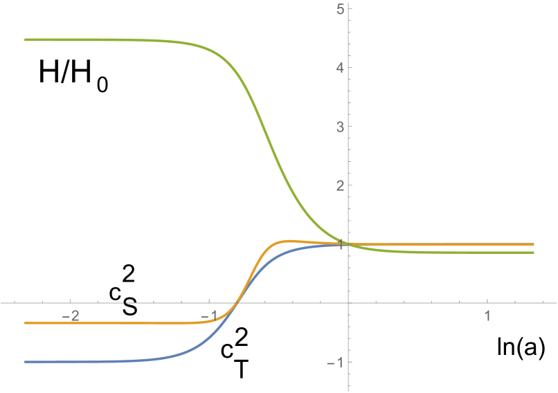
Figure 1: The dimensionless Hubble rate $\sqrt{y}=H/H_{0}$, the sound speeds squared in the scalar and tensor sectors against $\ln(a)$ for the isotropic $(Q_{\pm}=0)$ solution (4.12) with $\Omega_{0}=0.73$ and $\zeta=60$.

Setting $Q_{\pm}=0$ yields homogeneous and isotropic solutions, in which case one can apply the known formulas about describing small fluctuations. These formulas apply also for anisotropic solutions with $Q_{\pm}\neq 0$ at late and early times, when the solutions become isotropic. The quadratic action for fluctuations is

$$I=\frac{\mu}{2}\int{\rm K}\left(\dot{F}^{2}-c^{2}\frac{\rm p^{2}}{{\rm a}^{2}}\,F^{2}\right){\rm a}^{3}d^{4}x,$$ (4.16)

where $F$ denotes the fluctuation amplitude after separating the variables and ${\rm p}$ is the spatial momentum. The expressions for the kinetic term ${\rm K}$ and the sound speed squared $c^{2}$ within the model (4.7) were derived in [6], and they agree with the earlier result obtained within the generic Horndeski theory [13]. It turns out that the kinetic term is always positive, both in the tensor and scalar sectors, hence there are no ghosts. As seen in Fig.1, the sound speeds in both sectors are not constant, but they approach unity at late times. The deviation of the speed of tensor modes from unity at present is negligibly small and proportional to $(H_{\rm late}/H_{\rm early})^{2}$ [6].

It is also worth mentioning that, when written in the gauge where $G_{5}=0$ and hence $G_{4}=(\mu-\alpha X)/2$, the theory (4.7) can be mapped to Class I DHOST theory [25] via a disformal transformation of the metric $g_{\mu\nu}\to\tilde{g}_{\mu\nu}=A(X)\,g_{\mu\nu}+B(X)\,\nabla_{\mu}\phi\nabla_{\nu}\phi$. This transformation changes the light cone, hence the sound speeds change. If the functions $A,B$ are chosen such that $B(A-2XB)G_{4}=G_{4X}$ then the resulting DHOST theory will respect the condition which insures that the GW speed is equal to the speed of light (in the language of [26] this condition is $\alpha_{1}=\alpha_{2}=0$; see Eq.(D.5) of that work). Therefore, the GW speed can be made constant via the disformal transformation.

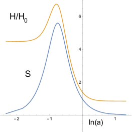
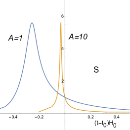
Figure 2: Left: the anisotropy amplitude ${\cal S}$ and the Hubble rate $H/H_{0}$ defined by (4.12),(4.13) with $\Omega_{0}=0.73$, $\zeta=60$ and ${\cal A}=\sqrt{Q_{+}^{2}+Q_{-}^{2}}=1$ against $\ln(a)$. Right: ${\cal S}(t)$ for ${\cal A}=1$ and ${\cal A}=10$.

The anisotropies are $s_{\pm}=Q_{\pm}{\cal S}$ where, as seen in Fig.2, the function ${\cal S}$ is well localized, hence the anisotropies vanish both at the early and late stages of the universe and are maximal in between. It is worth noting that, as seen in Fig.2, the anisotropies contribute to the Hubble rate and increase it. Since

$$dt=\frac{1}{H}\,d\ln(a),$$ (4.17)

the proper time interval $dt$ decreases if $H$ increases, hence the proper time duration of the anisotropic period decreases when the anisotropy amplitude ${\cal A}\equiv\sqrt{Q_{+}^{2}+Q_{-}^{2}}$ gets larger, since $H$ then increases. In other words, the function ${\cal S}(t)$ shows a more and more narrow peak when ${\cal A}$ gets larger, as seen in Fig.2.

One should emphasise that, although the anisotropies approach zero at early times, still the universe cannot be isotropic at this stage, since it is unstable in this limit with respect to inhomogeneous perturbations. This can be seen in Fig.1, which shows that the sound speeds squared become negative at early times. This means that the early stage of the universe should be inhomogeneous [6].

To recapitulate, the above example shows that anisotropies in the theory with ${\cal G}=\mu+\alpha\,X$ are damped at early times. It is possible that choosing other functions ${\cal G}(X)$ yields other models with a similar property. However, we shall now rather return to the original anisotropy equations (3.17) and (3.18) and consider situations when the nonlinear terms in these equations become important.

V The $G_{5}(X)$ case

Theories with a nontrivial $G_{5}(X)$ are also characterized by a non-constant GW speed. We shall consider a theory which also shows two inflationary stages, similarly to the $G_{4}(X)$ model considered above. It is defined by the choice

$$G_{2}=X-\Lambda,~{}~{}~{}~{}~{}~{}G_{3}=0,~{}~{}~{}~{}~{}G_{4}=\frac{1}{2}\,\mu,~{}~{}~{}~{}~{}~{}G_{5}=const+\xi\,\sqrt{2X}.$$ (5.1)

Equations (III),(3.17)-(III) then reduce to

$$3\mu\,(H^{2}-\dot{\beta}_{+}^{2}-\dot{\beta}_{-}^{2})+4\xi\,\dot{\phi}^{2}(2\dot{\beta}_{+}-H)[(H+\dot{\beta}_{+})^{2}-3\dot{\beta}_{-}^{2}] = \frac{1}{2}\,\dot{\phi}^{2}+\Lambda\,,$$

$$\dot{\phi}\left(-1+2\xi\,(2\dot{\beta}_{+}-H)[(H+\dot{\beta}_{+})^{2}-3\dot{\beta}_{-}^{2}]\right) = \frac{C_{\phi}}{{\rm a}^{3}}\,,$$

$$\left(\mu\dot{\beta}_{+}-\xi\,\dot{\phi}^{2}(\dot{\beta}_{+}^{2}+H\dot{\beta}_{+}-\dot{\beta}_{-}^{2})\right) = \frac{C_{+}}{{\rm a}^{3}}\,,$$

$$\left(\mu+\xi\,\dot{\phi}^{2}(2\dot{\beta}_{+}-H))\right)\dot{\beta}_{-} = \frac{C_{-}}{{\rm a}^{3}}\,,$$ (5.2)

all containing terms nonlinear in $\dot{\beta}_{\pm}$. Their dimensionless version is obtained by setting

$${\rm a}={\rm a}_{0}\,a,~{}~{}~{}H=H_{0}\,{y},~{}~{}~{}~{}\Lambda=3\mu H_{0}^{2}\Omega_{0},~{}~{}~{}~{}\xi=-\frac{1}{8H_{0}^{3}\zeta^{3}},$$

$$C_{\phi}=\sqrt{-\Omega_{6}\mu\xi H_{0}}\,H_{0}^{2}{\rm a}_{0}^{3},~{}~{}~{}~{}C_{\pm}=\mu H_{0}{\rm a}_{0}^{3}Q_{\pm}\,,~{}~{}~{}~{}\dot{\phi}=\sqrt{-\frac{\mu}{H_{0}\xi}}\,\psi\,,~{}~{}~{}~{}\dot{\beta}_{\pm}=H_{0}s_{\pm}\,,$$ (5.3)

where we assume that the coupling $\xi$ is negative, hence $\zeta>0$. This yields the equations

$$3\,(y^{2}-s_{+}^{2}-s_{-}^{2})+4\psi^{2}[(y-2s_{+})[(y+s_{+})^{2}-3s_{-}^{2}]-\zeta^{3}] = 3\Omega_{0}\,,$$

$$\left(4\zeta^{3}-(y-2s_{+})[(y+s_{+})^{2}-3s_{-}^{2}]\right)\psi = \frac{\sqrt{\Omega_{6}}}{2a^{3}},$$

$$\left(s_{+}+\psi^{2}[s_{+}^{2}+ys_{+}-s_{-}^{2}]\right) = \frac{Q_{+}}{a^{3}},$$

$$\left(1+\psi^{2}(y-2s_{+})]\right)s_{-} = \frac{Q_{-}}{a^{3}}.$$ (5.4)

Consider first the isotropic case,

$$s_{\pm}=0,~{}~{}~{}~{}Q_{\pm}=0.$$ (5.5)

Then equations (V) reduce to

$$3y^{2}+4\psi^{2}(y^{3}-\zeta^{3})=3\Omega_{0}\,,~{}~{}~{}~{}~{}~{}(4\zeta^{3}-y^{3})\psi=\frac{\sqrt{\Omega_{6}}}{2a^{3}},$$ (5.6)

with the solution

$$a^{6}=\frac{\Omega_{6}(\zeta^{3}-y^{3})}{3(4\zeta^{3}-y^{3})^{2}(y^{2}-\Omega_{0})},~{}~{}~{}~{}~{}~{}\psi=\frac{\sqrt{\Omega_{6}}}{2a^{3}(4\zeta^{3}-y^{3})}.$$ (5.7)

This solution again shows the early and late inflationary stages, since the Hubble parameter

$$\zeta\leftarrow y=\frac{H}{H_{0}}\rightarrow\sqrt{\Omega_{0}}~{}~{}~{}~{}\text{as}~{}~{}~{}~{}~{}0\leftarrow a\rightarrow\infty.$$ (5.8)

Requiring the solution to pass through the $a=y=1$ point yields

$$\Omega_{6}=\frac{3(4\zeta^{3}-1)^{2}(1-\Omega_{0})}{(\zeta^{3}-1)}.$$ (5.9)

Choosing $\Omega_{0}=0.7$ and $\zeta=5$ then yields

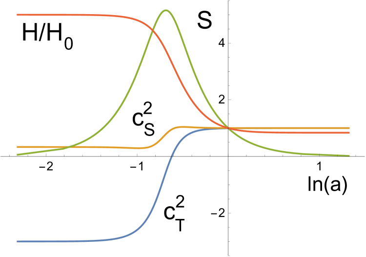
Figure 3: The Hubble rate, the sound speeds squared and the anisotropy amplitude ${\cal S}$ defined by (5.15) against $\ln(a)$ for the solution (5.7) with $\Omega_{0}=0.7$ and $\zeta=5$. The sound speed squared in the scalar sector is always positive. In the linear approximation assumed in (5.15) the anisotropies do not contribute to the Hubble rate.

the result shown in Fig.3. Remarkably, we see that the sound speed squared in the scalar sector is now always positive. The kinetic terms are also positive, and there remains only the gradient instability in the tensor sector at early times. Therefore, the theory is more stable than the $G_{4}(X)$ model considered above. This suggests that other choices of functions $G_{A}(X)$ may perhaps give completely stable theories, but this issue requires a separate analysis.

Equation (5.7) actually defines not one by two different solutions related to each other via $a\to-a$ and $\psi\to-\psi$, since $a^{3}=\pm\sqrt{a^{6}}$ can be either positive or negative whereas the metric contains only $a^{2}$ and is insensitive to the sign of $a$. As we shall see below, the anisotropic generalizations of these two solutions will no longer be related to each other in a simple way.

Let us consider anisotropic solutions of (V), starting from the simplest case where $Q_{\pm}=0$. The simplest solution is then the isotropic one,

$$s_{\pm}=0,$$ (5.10)

with $a$ and $\psi$ given by (5.7). In addition, since the equations are nonlinear in the anisotropies, there are also solutions with $s_{\pm}\neq 0$. They can be represented in the parametric form, choosing $\psi$ as the parameter:

$$a^{3}=\frac{\sqrt{\Omega_{6}}\,\psi^{5}}{4\zeta^{3}\psi^{6}-3\Omega_{0}\psi^{4}+1},~{}~{}~{}~{}~{}y=\frac{2}{3}\,\zeta^{3}\psi^{4}+\frac{1}{2}\Omega_{0}\psi^{2}-\frac{5}{6\psi^{2}},$$ (5.11)

with the anisotropies being either

$$s_{+}=\frac{1}{2}\left(y+\frac{1}{\psi^{2}}\right),~{}~{}~{}~{}s_{-}=\pm\sqrt{3}\,s_{+}\,,$$ (5.12)

or

$$s_{+}=-\left(y+\frac{1}{\psi^{2}}\right),~{}~{}~{}~{}s_{-}=0.$$ (5.13)

The parameter $\psi$ in (5.11) takes values in the interval $[0,\psi_{\rm m}]$ where $\psi_{\rm m}$ is the root of $4\zeta^{3}\psi^{6}-3\Omega_{0}\psi^{4}+1=0$. For example, if $\zeta=0.6$ and $\Omega_{0}=0.7$ then $\psi_{\rm m}=0.92$. When $\psi$ increases from zero to $\psi_{\rm m}$, the scale factor $a$ grows from zero to infinity, while the Hubble parameter $y$ and the anisotropy behave as follows:

$$\infty\leftarrow y\rightarrow\frac{1-\Omega_{0}\psi^{4}_{\rm m}}{\psi^{2}_{\rm m}},~{}~{}~{}~{}~{}~{}~{}~{}~{}-\infty\leftarrow y+\frac{1}{\psi^{2}}\rightarrow-\Omega_{0}\psi_{\rm m}^{2}~{}~{}~{}~{}~{}~{}~{}~{}~{}~{}~{}\text{as}~{}~{}~{}~{}~{}0\leftarrow a\rightarrow\infty.$$ (5.14)

We see that the anisotropies $s_{\pm}\sim(y+1/\psi^{2})$ do not vanish at late times but approach constant values, unless for $\Omega_{0}=0$. This again provides a counterexample to the standard wisdom. Indeed, in General Relativity the Bianchi universes with a positive cosmological constant always evolve toward an isotropic state at late times [4], [5]. The solution (5.11)-(5.14), although also containing a positive cosmological constant, shows just the opposite “self-anisotropizing” behaviour. It should be said that such a self-anisotropization in the Horndeski theory with a non-trivial $G_{5}(X)$ was actually detected before in Ref. [27], also when analyzing the Bianchi I models. We therefore shall not discuss this phenomenon anymore and simply refer to [27], since we are interested in the early time “isotropization” rather than in the late time “anisotropization”. For all other solutions that we consider in this text, apart from (5.11)-(5.14), the anisotropies always approach zero at late times. Therefore, we now return back to the isotropic solution (5.10) and consider its deformations induced by adding nonzero anisotropy charges $Q_{\pm}$.

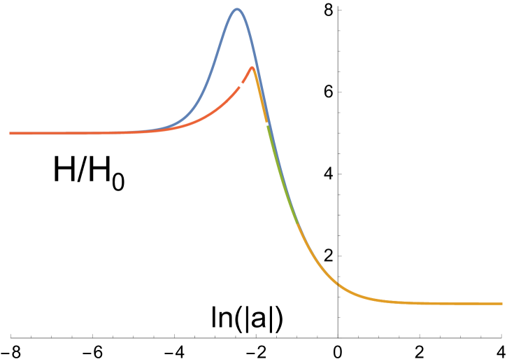
Figure 4: The Hubble rate $H/H_{0}=y=Y-s_{+}$ against $\ln(|a|)$ for the two solutions of (5.22) with $\Omega_{0}=0.7$, $\zeta=5$ for $S=0.02$. The Hubble rate is affected by the anisotropies when the nonlinear terms are taken into account.

If $Q_{\pm}$ are very small, then one can expect the anisotropies $s_{\pm}$ to be small as well, in which case one can neglect all nonlinear in $s_{\pm}$ terms in the equations. The first two equations in (V) contain only such terms, and neglecting them yields the equations of the isotropic case whose solution was described above by (5.7). The last two equations in (V) do contain terms linear in $s_{\pm}$, and keeping only these yields the solution

$$s_{\pm}=\frac{Q_{\pm}}{a^{3}(1+\psi^{2}y)}\equiv Q_{\pm}{\cal S},$$ (5.15)

with $a,\psi$ are given by (5.7). The function ${\cal S}$ here is well localized, as seen in Fig.3, and it has the following limits:

$$\frac{36\zeta^{5}}{\Omega_{6}}\,a^{3}\leftarrow{\cal S}\rightarrow\frac{1}{a^{3}}~{}~{}~{}~{}\text{as}~{}~{}~{}~{}~{}0\leftarrow a\rightarrow\infty.$$ (5.16)

Therefore, the anisotropies are suppressed both at early and late times.

If the charges $Q_{\pm}$ are not small, then one cannot neglect the nonlinear in anisotropies terms in the equations. It is not then obvious that the anisotropies will still be suppressed at early and late times. Let us therefore take the nonlinear terms into account. To simplify the analysis, we set one of the anisotropy amplitudes and the corresponding charge to zero,

$$s_{-}=Q_{-}=0,$$ (5.17)

while keeping $s_{+}\neq 0$ and denoting

$$Q_{+}=\sqrt{\Omega_{6}}\,S.$$ (5.18)

It turns out that all nonlinear in $s_{+}$ terms in the equations can be absorbed by introducing the new variable

$$Y=y+s_{+}.$$ (5.19)

Then equations (V) reduce, without any approximation, to

$$4\psi^{2}(Y^{3}-3Y^{2}s_{+}-\zeta^{3})+3Y^{2}-6Ys_{+} = 3\Omega_{0}\,,$$

$$\psi(4\zeta^{3}+3Y^{2}s_{+}-Y^{3}) = \frac{\sqrt{\Omega_{6}}}{2a^{3}}\,,$$

$$(Y\psi^{2}+1)s_{+} = \frac{S\sqrt{\Omega_{6}}}{a^{3}}.$$ (5.20)

Their solution is

$$a^{3}=\frac{\sqrt{\Omega_{6}}\,(6S\,Y^{2}\psi-Y\psi^{2}-1)}{2\psi(Y^{3}-4\zeta^{3})(Y\psi^{2}+1)},~{}~{}~{}~{}~{}~{}~{}~{}s_{+}=\frac{S\sqrt{\Omega_{6}}}{a^{3}(Y\psi^{2}+1)}\,,$$ (5.21)

where $Y$ and $\psi$ are related via

$$\psi^{2}=\frac{3}{4}\,\frac{Y^{2}-\Omega_{0}}{\zeta^{3}-Y^{3}}+\frac{3}{2}\,S\,Y\psi\frac{12\zeta^{3}Y\psi^{2}+Y^{3}+8\zeta^{3}-3\Omega_{0}Y}{(Y\psi^{2}+1)(Y^{3}-\zeta^{3})}.$$ (5.22)

If $S=0$ then $s_{+}=0$, $Y=y$, and these formulas reduce to (5.7) describing the isotropic solution with $y=Y\in[\sqrt{\Omega_{0}},\zeta]$. If $S\neq 0$ then (5.22) yields the fourth order algebraic equation for $\psi=\psi(Y)$. Fortunately, all of its four solutions can be found analytically. Each of them is real-valued only within a finite interval of $Y$, but combining these piecewise solutions together yields two global solutions which are smooth and real-valued everywhere in the interval $Y\in[\sqrt{\Omega_{0}},\zeta]$. These two solutions have opposite signs of $\psi$ and of $a$.

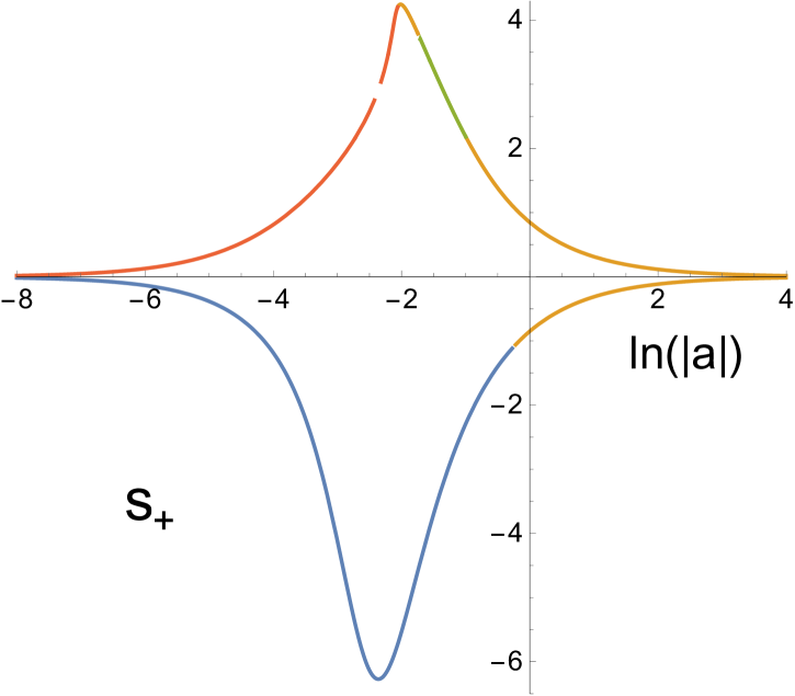
Figure 5: The anisotropy $s_{+}$ defined by (5.21) against $\ln(|a|)$ for the two solutions shown in Fig.4, assuming the normalizaton (5.9).

In the isotropic limit these two solutions are related by simply $\psi\to-\psi$ and $a\to-a$, as described above, while their Hubble rates $y(|a|)$ are the same. If $S\neq 0$ then the two solutions are no longer related to each other in a simple way and their Hubble rates are different, as seen in Figs.4. As seen in Fig.5, the anisotropies again vanish at late and early times. These nonlinear solutions were obtained for the value of the anisotropy parameter which is still small enough, $S=0.02$, but increasing $S$ does not qualitatively change the situation. Aalready for $S=1$ the anisotropy $s_{+}$ attains very large values in the intermediate region, but it always approaches zero as $a\to 0,\infty$. Therefore, the anisotropies are damped at early times also at the nonlinear level.

VI Conclusions

Summarizing the above discussion, we have studied homogeneous and anisotropic Bianchi I cosmologies within the most general Horndeski class. Our aim was to see whether the phenomenon of anisotropy damping previously observed within the specific Horndeski model [6] is present in other Horndeski theories as well. We have found the phenomenon to be absent for a large class of Horndeski models in which the GW speed is constant. However, the phenomenon seems to be generically present in the more general models with nontrivial $G_{4}(X)$ and/or $G_{5}(X)$. The GW speed in such theories is not constant, but no contradiction with the observation arises since the predicted value of the GW speed at present is extremely close to unity, whereas no observation data of the GW speed in the past are available.

Such theories show gradient instabilities at early times, therefore their initial phase, although not anisotropic, cannot be isotropic either. It should therefore be inhomogeneous. At the same time, it is possible that a systematic analysis of theories with more general $G_{4}(X,\phi)$ and/or $G_{5}(X,\phi)$ may reveal models free of instabilities. In the case of nonsingular bounce-type [28] or Genesis-type [29]) cosmologies, no stable solution can exist within the Horndeski class [30], [31], although they exist within the more general DHOST models (see [32] for a review). However, we are unaware of similar no-go results for cosmologies with an initial singularity. In fact, an explicit example of a completely stable Horndeski theory is known, although not containing an early inflationary phase [33]. Therefore, it is not excluded that stable cosmologies with the early and late inflationary phases may exist within the Horndeski theory, hence their anisotropies should be damped near singularity.

It should also be mentioned that, as was first observed in [6], the effect of anisotropy damping may be sensitive to the inclusion of spatial curvature.

- [1] V. A. Belinsky, I. M. Khalatnikov, and E. M. Lifshitz, Oscillatory approach to a singular point in the relativistic cosmology, Adv. Phys. 19 (1970) 525–573, [doi:10.1080/00018737000101171].
- [2] C. B. Collins and S. W. Hawking, Why is the Universe isotropic?, Astrophys. J. 180 (1973) 317–334, [doi:10.1086/151965].
- [3] V. A. Belinsky, I. M. Khalatnikov, and E. M. Lifshitz, A General Solution of the Einstein Equations with a Time Singularity, Adv. Phys. 31 (1982) 639–667, [doi:10.1080/00018738200101428].
- [4] A. A. Starobinsky, Isotropization of arbitrary cosmological expansion given an effective cosmological constant, JETP Lett. 37 (1983) 66–69.
- [5] R. M. Wald, Asymptotic behavior of homogeneous cosmological models in the presence of a positive cosmological constant, Phys. Rev. D28 (1983) 2118–2120, [doi:10.1103/PhysRevD.28.2118].
- [6] A. A. Starobinsky, S. V. Sushkov, and M. S. Volkov, Anisotropy screening in Horndeski cosmologies, Phys. Rev. D 101 (2020), no. 6 064039, [arXiv:1912.12320], [doi:10.1103/PhysRevD.101.064039].
- [7] G. W. Horndeski, Second-order scalar-tensor field equations in a four-dimensional space, Int.J.Theor.Phys. 10 (1974) 363–384, [doi:10.1007/BF01807638].
- [8] P. Creminelli and F. Vernizzi, Dark energy after GW170817 and GRB170817A, Phys. Rev. Lett. 119 (2017), no. 25 251302, [doi:10.1103/PhysRevLett.119.251302].
- [9] J. M. Ezquiaga and M. Zumalacarregui, Dark energy after GW170817: dead ends and the road ahead, Phys.Rev.Lett. 119 (2017), no. 25 251304, [doi:10.1103/PhysRevLett.119.251304].
- [10] T. Baker, E. Bellini, P. G. Ferreira, M. Lagos, J. Noller, and I. Sawicki, Strong constraints on cosmological gravity from GW170817 and GRB 170817A, Phys. Rev. Lett. 119 (2017), no. 25 251301, [doi:10.1103/PhysRevLett.119.251301].
- [11] LIGO Scientific, Virgo Collaboration, B. Abbott et al., GW170817: observation of gravitational waves from a binary neutron star inspiral, Phys. Rev. Lett. 119 (2017), no. 16 161101, [doi:10.1103/PhysRevLett.119.161101].
- [12] S. V. Sushkov, Exact cosmological solutions with nonminimal derivative coupling, Phys. Rev. D80 (2009) 103505, [doi:10.1103/PhysRevD.80.103505].
- [13] T. Kobayashi, M. Yamaguchi, and J. Yokoyama, Generalized G-inflation: Inflation with the most general second-order field equations, Prog. Theor. Phys. 126 (2011) 511–529, [arXiv:1105.5723], [doi:10.1143/PTP.126.511].
- [14] C. Armendariz-Picon, T. Damour, and V. F. Mukhanov, k - inflation, Phys. Lett. B 458 (1999) 209–218, [arXiv:hep-th/9904075], [doi:10.1016/S0370-2693(99)00603-6].
- [15] C. Deffayet, O. Pujolas, I. Sawicki, and A. Vikman, Imperfect dark energy from Kinetic Gravity Braiding, JCAP 1010 (2010) 026, [arXiv:1008.0048], [doi:10.1088/1475-7516/2010/10/026].
- [16] S. V. Sushkov, Realistic cosmological scenario with nonminimal kinetic coupling, Phys. Rev. D85 (2012) 123520, [doi:10.1103/PhysRevD.85.123520].
- [17] E. N. Saridakis and S. V. Sushkov, Quintessence and phantom cosmology with non-minimal derivative coupling, Phys. Rev. D81 (2010) 083510, [arXiv:1002.3478], [doi:10.1103/PhysRevD.81.083510].
- [18] M. A. Skugoreva, S. V. Sushkov, and A. V. Toporensky, Cosmology with nonminimal kinetic coupling and a power-law potential, Phys. Rev. D 88 (2013) 083539, [arXiv:1306.5090], [doi:10.1103/PhysRevD.88.083539]. [Erratum: Phys.Rev.D 88, 109906 (2013)].
- [19] C. Gao, When scalar field is kinetically coupled to the Einstein tensor, JCAP 06 (2010) 023, [arXiv:1002.4035], [doi:10.1088/1475-7516/2010/06/023].
- [20] L. N. Granda and W. Cardona, General Non-minimal Kinetic coupling to gravity, JCAP 07 (2010) 021, [arXiv:1005.2716], [doi:10.1088/1475-7516/2010/07/021].
- [21] H. M. Sadjadi, Super-acceleration in a nonminimal derivative coupling model, Phys.Rev.D 83 (2011) 107301, [doi:10.1103/PhysRevD.83.107301].
- [22] F. B. Banijamali A., Crossing of omega=-1 with tachyon and non-minimal derivative coupling , Phys.Lett.B 703 (2011) 366–369, [doi:10.1016/j.physletb.2011.07.080].
- [23] G. Gubitosi and E. V. Linder, Purely Kinetic Coupled Gravity, Phys. Lett. B 703 (2011) 113–118, [arXiv:1106.2815], [doi:10.1016/j.physletb.2011.07.066].
- [24] A. A. Starobinsky, S. V. Sushkov, and M. S. Volkov, The screening Horndeski cosmologies, JCAP 1606 (2016), no. 06 007, [doi:10.1088/1475-7516/2016/06/007].
- [25] D. Langlois, Dark energy and modified gravity in degenerate higher-order scalar–tensor (DHOST) theories: A review, Int. J. Mod. Phys. D 28 (2019), no. 05 1942006, [arXiv:1811.06271], [doi:10.1142/S0218271819420069].
- [26] D. Langlois, K. Noui, and H. Roussille, Quadratic DHOST theories revisited, arXiv:2012.10218.
- [27] H. W. H. Tahara, S. Nishi, T. Kobayashi, and J. Yokoyama, Self-anisotropizing inflationary universe in Horndeski theory and beyond, JCAP 07 (2018) 058, [arXiv:1805.00186], [doi:10.1088/1475-7516/2018/07/058].
- [28] D. Battefeld and P. Peter, A Critical Review of Classical Bouncing Cosmologies, Phys. Rept. 571 (2015) 1–66, [arXiv:1406.2790], [doi:10.1016/j.physrep.2014.12.004].
- [29] P. Creminelli, A. Nicolis, and E. Trincherini, Galilean Genesis: An Alternative to inflation, JCAP 11 (2010) 021, [arXiv:1007.0027], [doi:10.1088/1475-7516/2010/11/021].
- [30] M. Libanov, S. Mironov, and V. Rubakov, Generalized Galileons: instabilities of bouncing and Genesis cosmologies and modified Genesis, JCAP 08 (2016) 037, [arXiv:1605.05992], [doi:10.1088/1475-7516/2016/08/037].
- [31] T. Kobayashi, Generic instabilities of nonsingular cosmologies in Horndeski theory: A no-go theorem, Phys. Rev. D 94 (2016), no. 4 043511, [arXiv:1606.05831], [doi:10.1103/PhysRevD.94.043511].
- [32] S. Mironov, V. Rubakov, and V. Volkova, Cosmological scenarios with bounce and Genesis in Horndeski theory and beyond: An essay in honor of I.M. Khalatnikov on the occasion of his 100th birthday, arXiv:1906.12139, doi:10.1134/S0044451019100079.
- [33] G. Koutsoumbas, K. Ntrekis, E. Papantonopoulos, and E. N. Saridakis, Unification of Dark Matter - Dark Energy in Generalized Galileon Theories, JCAP 02 (2018) 003, [arXiv:1704.08640], [doi:10.1088/1475-7516/2018/02/003].