Probabilistic Learning on Manifolds (PLoM) with Partition

Abstract

The probabilistic learning on manifolds (PLoM) introduced in 2016 has solved difficult supervised problems for the “small data” limit where the number $N$ of points in the training set is small. Many extensions have since been proposed, making it possible to deal with increasingly complex cases. However, the performance limit has been observed and explained for applications for which $N$ is very small ($50$ for example) and for which the dimension of the diffusion-map basis is close to $N$. For these cases, we propose a novel extension based on the introduction of a partition in independent random vectors. We take advantage of this novel development to present improvements of the PLoM such as a simplified algorithm for constructing the diffusion-map basis and a new mathematical result for quantifying the concentration of the probability measure in terms of a probability upper bound. The analysis of the efficiency of this novel extension is presented through two applications.

Notations

The following notations are used:
A lower case letter such as $x$, $\eta$, or $u$, is a real deterministic variable.
A boldface lower case letter such as x, ${\boldsymbol{\eta}}$, or u is a real deterministic vector.
An upper case letter such as $X$, ${\rm H}$, or $U$, is a real random variable (except for $E$).
A boldface upper case letter, X, H, or U, is a real random vector.
A letter between brackets such as $[x]$, $[\eta]$, $[u]$ or $[C]$, is a real deterministic matrix.
A boldface upper case letter between brackets such as $[{\textbf{X}}]$, $[{{\textbf{H}}}]$, or $[{\textbf{U}}]$, is a real random matrix.
$n,n_{q},n_{u},n_{w}\,$: dimensions of random vectors ${\textbf{X}},{\textbf{Q}},{\textbf{U}},{\textbf{W}}$.
$n_{\hbox{{\ppppcarac MC}}}\,$: number of additional realizations for random matrix $[{\textbf{H}}^{N}_{m_{\hbox{{\ppppcarac o}}}}]$.
$n_{p}\,$: number of groups in the partition of H.
$m,m_{i}\,$: dimension of the reduced-order diffusion-map bases $[g_{m}],[g^{i}_{m}]$.
$m_{\hbox{{\ppcarac o}}},m_{i,{\hbox{{\ppcarac o}}}}\,$: optimal value of $m,m_{i}$.
$E\,$: mathematical expectation.
$N,N_{\hbox{{\pppcarac ar}}}\,$: number of points in the training, learned sets.
$\nu,\nu_{i}\,$: dimensions of random vectors ${\textbf{H}},{\textbf{Y}}^{i}$.
${\mathbb{R}},{\mathbb{R}}^{n}\,$: real line, Euclidean vector space of dimension $n$.
${\mathbb{M}}_{n},{\mathbb{M}}_{n,N}\,$: sets of all the $(n\times n),(n\times N)$ real matrices.
${\mathbb{M}}_{n}^{+}\,$: set of all the positive-definite symmetric $(n\times n)$ real matrices.
$\|{\textbf{x}}\|\,$: Euclidean norm when x is the vector or Frobenius norm when $[x]$ is the matrix.

1 Introduction

(i) About the PLoM

The PLoM (probabilistic learning on manifolds) method was proposed in 2016 [1] as a complementary approach to existing methods in machine learning. It allows for solving unsupervised and supervised problems under uncertainty for which the training sets are small. This situation is encountered in many problems of physics and engineering sciences with expensive function evaluations. The exploration of the admissible solution space in these situations is thus hampered by available computational resources. The PLoM was successfully adapted to tackle these challenges for several related problems including nonconvex optimization under uncertainty [2, 3] and the calculation of Sobol’s indices [4].

(ii) Brief discussion on the hypotheses on which the PLoM method has been built

The PLoM approach starts from a training set made up of a relatively small number $N$ of points (initial realizations). For the supervised case, it is assumed that the training set is related to an underlying stochastic manifold related to a ${\mathbb{R}}^{n}$-valued random variable ${\textbf{X}}=({\textbf{Q}},{\textbf{W}})$ with ${\textbf{Q}}={\textbf{f}}({\textbf{U}},{\textbf{W}})={\textbf{F}}({\textbf{W}})$. The measurable mapping f is unknown and F is also an unknown stochastic mapping. The probability distributions of the vector-valued random variables W (control parameter) and U (non-controlled parameter) are given. The stochastic manifold is defined by the unknown graph $\{{\textbf{w}},{\textbf{F}}({\textbf{w}})\}$ for w belonging to the support of the probability distribution of W. In the PLoM construction, its is not assumed that this stochastic manifold can directly be described; for instance, it is not assumed that there exist properties of local differentiability (moreover, the manifold is stochastic). Under these conditions, the probability measure of X is concentrated in a region of ${\mathbb{R}}^{n}$ for which the only available information is the cloud of the points of the training set. The PLoM method makes it possible to generate the learned set whose $n_{\hbox{{\pppcarac ar}}}\gg N$ points (additional realizations) are generated by the probability measure that is estimated from the training set. The concentration of the probability measure is preserved thanks to the use of the diffusion-maps basis that allows to enrich the available information from the training set. It should also be noted that the estimate of this unknown probability measure cannot be performed from the training set by using an arbitrarily estimator. It must be parameterized in a manner that permits convergence to any probability measure as its number of points goes towards infinity. The PLoM method therefore does not only consist in generating points that belong to the region in which the measure is concentrated, but also allows these additional points to be realizations of the estimate probability measure with the convergence properties evoked above. The choice of the kernel estimation method for estimating the probability measure from the training set guarantees that this required fundamental property is satisfied (see [1] and in particular, Section 5.3 of [5]).

(iii) A difficulty of the PLoM method for certain applications

Since its introduction in 2016, extensions of the original method [1] have been developed in order to address increasingly complex problems for the case of small data: sampling of Bayesian posteriors with a non-Gaussian probabilistic learning on manifolds in very high dimension [6], physics-constrained non-Gaussian probabilistic learning on manifolds, for instance, to integrate information coming from experimental measurements during the learning [7], probabilistic learning on manifolds constrained by nonlinear partial differential equations for small data [8]. During this period, a number of applications were addressed making it possible to refine the method, to validate it, and to better assess and relax its limitations. However, some challenges have remained. These are cases where the number of points (realizations) in the training set is very small (for example $50$) and for which the dimension of the subspace generated by the diffusion-map basis is very close to this number. In this case, the PLoM may not be more efficient than a standard MCMC algorithm that is agnostic to any concentration of the probability measure. One possible way to improve the PLoM for these very challenging cases is to partition the random vector of which the training set is a realization, into statistically independent groups in a non-Gaussian framework. In this manner, statistical knowledge about the data set, beyond its localization to a manifold, is relied upon to enhance information extraction and representation. One difficulty with standard grouping into independent components is that they typically divvy-up available samples into seperate groups, with each group consisting of a smaller number of samples. These approach would not be suitable to the present setting given the already small sample size or the training set. A more useful approach, which is adopted in this paper, results in groups that are each equal in size to the training set, but for which the dimension of the diffusion-map basis is significantly reduced. This approach corresponds to the novel extension of the PLoM method that we present in this paper.

(iv) A novel extension of the PLOM method to get around the difficulty

One of the ingredients for this novel extension of the PLoM method is the construction of a partition in non-Gaussian independent random vectors, assuming that it exists. Indeed, there may very well be applications for which the partition yields a single group, identical to the initial random vector. For such cases the present approach of PLoM with partitions affords no further reduction. Concerning the construction of a partition of independent random vectors, a popular method for testing the statistical independence of the $\nu$ components of a random vector from a given set of $N$ realizations is the use of the frequency distribution [9] coupled with the use of the Pearson chi-squared ($\chi^{2}$) test [10, 11]. For the high dimensions ($\nu$ big) and a relatively small value of $N$, such an approach does not give sufficiently accurate results. In addition, even when this type of methods permits testing for independence, the need remains for a fast algorithm for constructing the optimal partition . The independent component analysis (ICA) [12, 13, 14, 15, 16, 17, 18, 19] is a method that consists of extracting independent source signals as a linear mixture of mutually statistically dependent signals, and is often used for source-separation problems. The fundamental hypothesis that introduced in the ICA methodology is that the observed vector-valued signal is a linear transformation of statistically independent real-valued signals (that is to say, is a linear transformation of a vector-valued signal whose components are mutually independent) and the objective of the ICA algorithms is to identify the best linear operator. In this paper, for the PLoM with partition, we use the procedure proposed in [20], which is an ICA by mutual information and which does not use the construction of a linear transformation. This direct algorithm permits the identification of an optimal partition in terms of independent random vectors for any non-Gaussian vector in high dimension, which is defined by a relatively small number $N$ of realizations, and which is based on Information Theory.

(v) Organization of the paper

In Section 2, we present the methodology of the PLoM method with partition. In the process, we reintroduce some necessary key notions of the PLoM method. Sections 3 and 4 are both devoted toapplications. Finally, a discussion of the method is presented in the conclusions.

(vi) Novelties presented in the paper

The main novelty is the development of the PLoM methodology with partition. We also propose a novel algorithm for identifying the optimal values of the hyperparameters related to the construction of the reduced-order diffusion-map basis. For covering the cases for which the normalization introduced by the PLoM is lost with the use of a partition, we introduce constraints by using the Kullback-Leibler minimum cross-entropy principle [7]. The quantification of the concentration of the probability measure for the PLoM, which is performed with the distance introduced in [5], is extended for the PLoM with partition, and is completed by a novel result formulated in terms of a probability upper bound of the measure of concentration.

2 Methodology

2.1 Supervised problem and training set

Let $({\textbf{w}},{\textbf{u}})\mapsto{\textbf{f}}({\textbf{w}},{\textbf{u}})$ be any measurable mapping on ${\mathbb{R}}^{n_{w}}\times{\mathbb{R}}^{n_{u}}$ with values in ${\mathbb{R}}^{n_{q}}$ representing a mathematical/computational model. Let W be the ${\mathbb{R}}^{n_{w}}$-valued random control parameter and let U be a ${\mathbb{R}}^{n_{u}}$-valued random non-controlled parameter, defined on a probability space $(\Theta,{\mathcal{T}},{\mathcal{P}})$. The random vectors W and U are assumed to be statistically independent and they are generally non-Gaussian. The probability distributions $P_{\textbf{W}}(d{\textbf{w}})$ $=p_{\textbf{W}}({\textbf{w}})\,d{\textbf{w}}$ and $P_{\textbf{U}}(d{\textbf{u}})=p_{\textbf{U}}({\textbf{u}})\,d{\textbf{u}}$ are defined by the probability density functions $p_{\textbf{W}}$ and $p_{\textbf{U}}$ with respect to the Lebesgue measures $d{\textbf{w}}$ and $d{\textbf{u}}$ on ${\mathbb{R}}^{n_{w}}$ and ${\mathbb{R}}^{n_{u}}$. Let Q be the ${\mathbb{R}}^{n_{q}}$-valued random variable (QoI) defined on $(\Theta,{\mathcal{T}},{\mathcal{P}})$ such that ${\textbf{Q}}={\textbf{f}}({\textbf{W}},{\textbf{U}})$. It is assumed that $N\geq 3$ independent realizations $\{{\textbf{q}}_{d}^{j},j=1,\ldots,N\}$ of Q have been computed such that ${\textbf{q}}_{d}^{j}={\textbf{f}}({\textbf{w}}_{d}^{j},{\textbf{u}}_{d}^{j})$ in which $\{{\textbf{w}}_{d}^{j},j=1,\ldots,N\}$ and $\{{\textbf{u}}_{d}^{j},j=1,\ldots,N\}$ are $N$ independent realizations of W and U (subscript $d$ refers to the training set). We then consider the random variable X with values in ${\mathbb{R}}^{n}$, such that ${\textbf{X}}=({\textbf{Q}},{\textbf{W}})$ with $n=n_{q}+n_{w}$. The training set (initial data set) related to random vector X is then made up of the $N$ independent realizations $\{{\textbf{x}}_{d}^{j},j=1,\ldots,N\}$ in which ${\textbf{x}}_{d}^{j}=({\textbf{q}}_{d}^{j},{\textbf{w}}_{d}^{j})\in{\mathbb{R}}^{n}$ (note that U is not included in X). Since generally the data pertains to heterogeneous features with potentially wildly distinct supports, it is assumed that the training set has been suitably scaled for the purpose of computational statistics. Let us assume that the measurable mapping f is such that the conditional probability distribution $P_{{\textbf{Q}}|{\textbf{W}}}(d{\textbf{q}}|{\textbf{w}})$ given ${\textbf{W}}={\textbf{w}}$ admits a conditional probability density function. It can be deduced (see [7]) that the probability distribution $P_{\textbf{X}}(d{\textbf{x}})$ of X admits a density ${\textbf{x}}\mapsto p_{\textbf{X}}({\textbf{x}})$ with respect to the Lebesgue measure $d{\textbf{x}}$ on ${\mathbb{R}}^{n}$. The PLoM [1, 5] allows for generating the learned set made up of $N_{\hbox{{\pppcarac ar}}}\gg N$ realizations $\{{\textbf{x}}_{\hbox{{\pppcarac ar}}}^{\ell},\ell=1,\ldots,N_{\hbox{{\pppcarac ar}}}\}$ that allows for deducing $\{({\textbf{q}}_{\hbox{{\pppcarac ar}}}^{\ell},{\textbf{w}}_{\hbox{{\pppcarac ar}}}^{\ell})={\textbf{x}}_{\hbox{{\pppcarac ar}}}^{\ell},\ell=1,\ldots,N_{\hbox{{\pppcarac ar}}}\}$ without using the computational model, but using only the training set (subscript $ar$ refers to the learned set).

2.2 Principal component analysis (PCA) of random vector X

Let $\underline{{\textbf{x}}}_{d}\in{\mathbb{R}}^{n}$ and $[C_{\textbf{X}}]\in{\mathbb{M}}_{n}^{+}$ be the mean vector and the covariance matrix of X estimated with the training set. Let $\mu_{1}\geq\mu_{2}\geq\ldots\geq\mu_{\nu}>0$ be the $\nu$ largest eigenvalues and let ${\boldsymbol{\varphi}}^{1},\ldots,{\boldsymbol{\varphi}}^{\nu}$ be the associated orthonormal eigenvectors of $[C_{\textbf{X}}]$. The integer $\nu\leq n$ is such that, for a given $\varepsilon_{\hbox{{\pppppcarac PCA}}}>0$, we have ${\hbox{{\pcarac err}}}_{\hbox{{\pppppcarac PCA}}}(\nu)=1-{\sum_{\alpha=1}^{\nu}\mu_{\alpha}}/{{\hbox{{{t}r}}}[C_{\textbf{X}}]}\leq\varepsilon_{\hbox{{\pppppcarac PCA}}}$. The PCA of X allows for representing X by ${\textbf{X}}^{\nu}$ such that ${\textbf{X}}^{\nu}=\underline{{\textbf{x}}}_{d}+[\Phi]\,[\mu]^{1/2}\,{\textbf{H}}$ such that $E\{\|{\textbf{X}}-{\textbf{X}}^{\nu}\|^{2}\}\leq\varepsilon_{\hbox{{\pppppcarac PCA}}}\,E\{\|{\textbf{X}}\|^{2}\}$, in which $[\Phi]=[{\boldsymbol{\varphi}}^{1}\ldots{\boldsymbol{\varphi}}^{\nu}]\in{\mathbb{M}}_{n,\nu}$ such that $[\Phi]^{T}\,[\Phi]=[I_{\nu}]$ and $[\mu]$ is the diagonal $(\nu\times\nu)$ matrix such that $[\mu]_{\alpha\beta}=\mu_{\alpha}\delta_{\alpha\beta}$. From a numerical point of view, if $N<n$, then matrix $[C_{\textbf{X}}]$ is not estimated and $\nu,[\mu]$, and $[\Phi]$ are directly computed using a thin SVD [21] of the matrix whose $N$ columns are $({\textbf{x}}_{d}^{j}-\underline{{\textbf{x}}}_{d})$ for $j=1,\ldots,N$. The ${\mathbb{R}}^{\nu}$-valued random variable H is obtained by projection, ${\textbf{H}}=[\mu]^{-1/2}\,[\Phi]^{T}\,({\textbf{X}}-\underline{{\textbf{x}}}_{d})$, and its $N$ independent realizations $\{{\boldsymbol{\eta}}_{d}^{j},j=1,\ldots,N\}$ are such that ${\boldsymbol{\eta}}_{d}^{j}=[\mu]^{-1/2}\,[\Phi]^{T}\,({\textbf{x}}_{d}^{j}-\underline{{\textbf{x}}}_{d})\in{\mathbb{R}}^{\nu}$. Using $\{{\boldsymbol{\eta}}_{d}^{j},j=1,\ldots,N\}$, the estimates of the mean vector and the covariance matrix of H verify $\underline{{\boldsymbol{\eta}}}_{d}={\hbox{\bf 0}}_{\nu}$ and $[C_{\textbf{H}}]=[I_{\nu}]$. We define the matrix $[\eta_{d}]=[{\boldsymbol{\eta}}_{d}^{1}\ldots{\boldsymbol{\eta}}_{d}^{N}]\in{\mathbb{M}}_{\nu,N}$ whose columns are the $N$ realizations of H, which is such that

$$\|[\eta_{d}]\|^{2}={\hbox{{{t}r}}}\{[\eta_{d}]^{T}\,[\eta_{d}]\}=\sum_{j=1}^{N}\|{\boldsymbol{\eta}}_{d}^{j}\|^{2}=\nu(N-1)\,.$$ (1)

2.3 PLoM method with no group (No-Group PLoM)

The PLoM analysis used is the one presented in [1] whose complete mathematical analysis is performed in [5].

2.3.1 Nonparametric estimate of the pdf of H

A modification of the multidimensional Gaussian kernel-density estimation method [22, 23, 24, 25] is used for constructing the nonparametric estimate $p_{\textbf{H}}^{(N)}$ on ${\mathbb{R}}^{\nu}$ of the pdf $p_{\textbf{H}}$ of random vector H, which is written (see Theorem 3.1 of [5] for the convergence with respect to $N$) as

$$p_{\textbf{H}}^{(N)}({\boldsymbol{\eta}})=\frac{1}{N}\sum_{j=1}^{N}\,\frac{1}{(\sqrt{2\pi}\,\widehat{s})^{\nu}}\,\exp\{-\frac{1}{2\widehat{s}^{2}}\|\frac{\widehat{s}}{s}\,{\boldsymbol{\eta}}_{d}^{j}-{\boldsymbol{\eta}}\|^{2}\}\quad,\quad\forall{\boldsymbol{\eta}}\in{\mathbb{R}}^{\nu}\,,$$ (2)

in which $s=(N(\nu+2)/4)^{-{1}/{(\nu+4)}}$ is the usual Silverman bandwidth (since $[C_{\textbf{H}}]=[I_{\nu}]$, see for instance, [26]) and where $\widehat{s}=s\,(s^{2}\!+\!(N\!-\!1)/{N})^{-1/2}$ has been introduced in order that $\int_{{\mathbb{R}}^{\nu}}{\boldsymbol{\eta}}\,p_{\textbf{H}}^{(N)}({\boldsymbol{\eta}})\,d{\boldsymbol{\eta}}=0_{\nu}$ and $\int_{{\mathbb{R}}^{\nu}}{\boldsymbol{\eta}}\otimes{\boldsymbol{\eta}}\,\,p_{\textbf{H}}^{(N)}({\boldsymbol{\eta}})\,d{\boldsymbol{\eta}}=[I_{\nu}]$.

2.3.2 Construction of a reduced-order diffusion-map basis (ROB-DM)

To identify the subset around which the initial data are concentrated, the PLoM relies on the diffusion-map method [27, 28]. The Gaussian kernel is used. Let $[K]$ and $[b]$ be the matrices such that, for all $i$ and $j$ in $\{1,\ldots,N\}$, $[K]_{ij}=\exp\{-(4\,\varepsilon_{\hbox{{\pppppcarac DM}}})^{-1}\|{\boldsymbol{\eta}}_{d}^{i}-{\boldsymbol{\eta}}_{d}^{j}\|^{2}\}$ and $[b]_{ij}=\delta_{ij}\,b_{i}$ with $b_{i}=\sum_{j=1}^{N}[K]_{ij}$, in which $\varepsilon_{\hbox{{\pppppcarac DM}}}>0$ is a smoothing parameter (the non symmetric matrix ${\mathbb{P}}=[b]^{-1}[K]\in{\mathbb{M}}_{N}$ is the transition matrix of a Markov chain that yields the probability of transition in one step). The eigenvalues $\lambda_{1},\ldots,\lambda_{N}$ and the associated eigenvectors ${\boldsymbol{\psi}}^{1},\ldots,{\boldsymbol{\psi}}^{N}$ of the right-eigenvalue problem $[{\mathbb{P}}]\,{\boldsymbol{\psi}}^{\alpha}=\lambda_{\alpha}\,{\boldsymbol{\psi}}^{\alpha}$ are such that $1=\lambda_{1}>\lambda_{2}\geq\ldots\geq\lambda_{N}$ and are computed by solving the generalized eigenvalue problem $[K]\,{\boldsymbol{\psi}}^{\alpha}=\lambda_{\alpha}\,[b]\,{\boldsymbol{\psi}}^{\alpha}$ with the normalization $<\![b]\,{\boldsymbol{\psi}}^{\alpha},{\boldsymbol{\psi}}^{\beta}\!>=\delta_{\alpha\beta}$. The eigenvector ${\boldsymbol{\psi}}^{1}$ associated with $\lambda_{1}=1$ is a constant vector. For a given integer $\kappa\geq 0$, the diffusion-map basis $\{{\textbf{g}}^{1},\ldots,{\textbf{g}}^{\alpha},\ldots,{\textbf{g}}^{N}\}$ is a vector basis of ${\mathbb{R}}^{N}$ defined by ${\textbf{g}}^{\alpha}=\lambda^{\kappa}_{\alpha}\,{\boldsymbol{\psi}}^{\alpha}$. For a given integer $m$ with $3\leq m\leq N$, the reduced-order diffusion-map basis of order $m$ is defined as the family $\{{\textbf{g}}^{1},\ldots,{\textbf{g}}^{m}\}$ that is represented by the matrix $[g_{m}]=[{\textbf{g}}^{1}\ldots{\textbf{g}}^{m}]\in{\mathbb{M}}_{N,m}$ with ${\textbf{g}}^{\alpha}=(g_{1}^{\alpha},\ldots,g_{N}^{\alpha})$ and $[g_{m}]_{\ell\alpha}=g_{\ell}^{\alpha}$. This ROB-DM depends on two parameters, $\varepsilon_{\hbox{{\pppppcarac DM}}}$ and $m$, which have to be identified. It is proven in [5], that the PLoM method does not depend of $\kappa$ that can therefore be chosen to $0$.

It should be noted that, if $\nu=1$, then there is no really interest to use the ROB-DM and in this case, we propose to take $m=N$ and $[g_{N}]=[I_{N}]$. For non-trivial applications analyzed with the PLoM without partition, we always have $\nu>1$ and even, $1\ll\nu\leq n$. However for the PLoM method with partition, optimal partitions can be found for which some groups may have dimension $1$ (hence the consideration of possible cases of this type).

2.3.3 Novel algorithm for identifying the optimal values $\varepsilon_{\hbox{{\ppcarac o}}}$ and $m_{\hbox{{\ppcarac o}}}$ of $\varepsilon_{\hbox{{\pppppcarac DM}}}$ and $m$

Let us assume that $\nu\geq 2$. For estimating the optimal values $\varepsilon_{\hbox{{\ppcarac o}}}$ of $\varepsilon_{\hbox{{\pppppcarac DM}}}$ and $m_{\hbox{{\ppcarac o}}}$ of $m$, the criterion of the eigenvalues given in Section 5.2 of [5] must be satisfied for the PLoM method to be applicable. This criterion can be summarized as follows. We have to find the value $m_{\hbox{{\ppcarac o}}}\leq N$ of $m$ and the smallest value $\varepsilon_{\hbox{{\ppcarac o}}}>0$ of $\varepsilon_{\hbox{{\pppppcarac DM}}}$ such that

$$1=\lambda_{1}>\lambda_{2}(\varepsilon_{\hbox{{\ppcarac o}}})\simeq\ldots\simeq\lambda_{m_{\hbox{{\ppppcarac o}}}}(\varepsilon_{\hbox{{\ppcarac o}}})\gg\lambda_{m_{\hbox{{\ppppcarac o}}}+1}(\varepsilon_{\hbox{{\ppcarac o}}})\geq\ldots\geq\lambda_{N}(\varepsilon_{\hbox{{\ppcarac o}}})>0\,,$$ (3)

with a jump in amplitude equal to $10$ between $\lambda_{m_{\hbox{{\ppppcarac o}}}}(\varepsilon_{\hbox{{\ppcarac o}}})$ and $\lambda_{m_{\hbox{{\ppppcarac o}}}+1}(\varepsilon_{\hbox{{\ppcarac o}}})$. This property means that we have to find $m_{\hbox{{\ppcarac o}}}\leq N$ and the smallest positive value $\varepsilon_{\hbox{{\ppcarac o}}}$ in order (i) to have $\lambda_{2}(\varepsilon_{\hbox{{\ppcarac o}}})<1$ (one must not have several eigenvalues in the neighborhood of $1$) and (ii) to obtain a plateau for $\lambda_{2}(\varepsilon_{\hbox{{\ppcarac o}}})$ to $\lambda_{m_{\hbox{{\ppppcarac o}}}}(\varepsilon_{\hbox{{\ppcarac o}}})$ with a jump of amplitude $10$ between $\lambda_{m_{\hbox{{\ppppcarac o}}}}(\varepsilon_{\hbox{{\ppcarac o}}})$ and $\lambda_{m_{\hbox{{\ppppcarac o}}}+1}(\varepsilon_{\hbox{{\ppcarac o}}})$. A further in-depth analysis makes it possible to state the following new criterion and algorithm to easily estimate $\varepsilon_{\hbox{{\ppcarac o}}}$ and $m_{\hbox{{\ppcarac o}}}$. Let $\varepsilon_{\hbox{{\pppppcarac DM}}}\mapsto{\hbox{{\ppcarac Jump}}}(\varepsilon_{\hbox{{\pppppcarac DM}}})$ be the function on $]0,+\infty[$ defined by ${\hbox{{\ppcarac Jump}}}(\varepsilon_{\hbox{{\pppppcarac DM}}})=\lambda_{m_{\hbox{{\ppppcarac o}}}+1}(\varepsilon_{\hbox{{\pppppcarac DM}}})/\lambda_{2}(\varepsilon_{\hbox{{\pppppcarac DM}}})$.

Algorithm 1 Algorithm for estimating the optimal values $m_{\hbox{{\ppcarac o}}}$ of $m$ and $\varepsilon_{\hbox{{\ppcarac o}}}$ of $\varepsilon_{\hbox{{\pppppcarac DM}}}$

1:  if $\nu=1$ then

2:     Set the value of $m$ to $m_{\hbox{{\ppcarac o}}}=N$ and $[g_{N}]=[I_{N}]$.

3:  end if

4:  if $\nu\geq 2$ then

5:     Set the value of $m$ to $m_{\hbox{{\ppcarac o}}}=\nu+1$.

6:     Identify the smallest possible value $\varepsilon_{\hbox{{\ppcarac o}}}$ of $\varepsilon_{\hbox{{\pppppcarac DM}}}$ in order that ${\hbox{{\ppcarac Jump}}}(\varepsilon_{\hbox{{\ppcarac o}}})\leq 0.1$ and such that Eq. (3) be verified.

7:  end if

The novel algorithm is thus given in Algorithm 1 and Figure 1 shows an illustration: we have $m_{\hbox{{\ppcarac o}}}=\nu+1=61$; the optimal value of $\varepsilon_{\hbox{{\pppppcarac DM}}}$ that satisfies the criteria is $\varepsilon_{\hbox{{\ppcarac o}}}=65$ and yields Figure 1a; if a smaller value than $65$ is chosen, for instance the value $5$, then there will be many eigenvalues close to $1$ as shown in Figure 1b; if the smallest value for $\varepsilon_{\hbox{{\pppppcarac DM}}}$ is not selected, for example taking the value $100$, then the plateau is not obtained as shown in Figure 1c. For these two bad values of $\varepsilon_{\hbox{{\pppppcarac DM}}}$, the calculated diffusion-map basis is not adapted to the PLoM procedure.

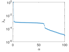
(a) Correct value $\varepsilon_{\hbox{{\ppcarac o}}}$ of $\varepsilon_{\hbox{{\pppppcarac DM}}}$

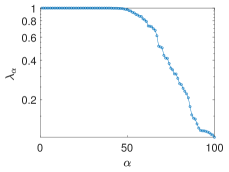
(b) Bad value of $\varepsilon_{\hbox{{\pppppcarac DM}}}$ that is smaller than $\varepsilon_{\hbox{{\ppcarac o}}}$

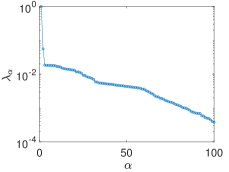
(c) Bad value of $\varepsilon_{\hbox{{\pppppcarac DM}}}$ that is larger than $\varepsilon_{\hbox{{\ppcarac o}}}$

Figure 1: Illustration of the criterion effects defined by Eq. (3) for identifying $\varepsilon_{\hbox{{\ppcarac o}}}$.

2.3.4 Random matrices $[\,{\textbf{H}}^{N}]$, $[\,{\textbf{H}}^{N}_{m}]$, $[\,{\textbf{H}}^{N}_{m_{\hbox{{\ppppcarac o}}}}]$, and MCMC generator

Let ${\textbf{H}}^{(N)}$ be the ${\mathbb{R}}^{\nu}$-valued random variable defined on $(\Theta,{\mathcal{T}},{\mathcal{P}})$ for which the pdf is $p_{\textbf{H}}^{(N)}$ defined by Eq. (2). Let $[{\textbf{H}}^{N}]$ be the random matrix with values in ${\mathbb{M}}_{\nu,N}$ such that $[{\textbf{H}}^{N}]=[{\textbf{H}}^{1}\ldots{\textbf{H}}^{N}]$ in which ${\textbf{H}}^{1},\ldots,{\textbf{H}}^{N}$ are $N$ independent copies of ${\textbf{H}}^{(N)}$. It can be seen that $E\{{\textbf{H}}^{(N)}\}={\hbox{\bf 0}}_{\nu}$ and $E\{{\textbf{H}}^{(N)}\otimes{\textbf{H}}^{(N)}\}=[I_{\nu}]$. Note that ${\textbf{H}}^{1},\ldots,{\textbf{H}}^{N}$ are not taken as $N$ independent copies of H whose pdf $p_{\textbf{H}}$ is unknown, but are taken as $N$ independent copies of ${\textbf{H}}^{(N)}$ whose pdf $p_{\textbf{H}}^{(N)}$ is known. The PLoM method introduces the ${\mathbb{M}}_{\nu,N}$-valued random matrix $[{\textbf{H}}^{N}_{m}]=[{\textbf{Z}}_{m}]\,[g_{m}]^{T}$ with $3\leq m\leq N$ , corresponding to a data-reduction representation of random matrix $[{\textbf{H}}^{N}]$, in which $[g_{m}]$ is the ROB-DM and where $[{\textbf{Z}}_{m}]$ is a ${\mathbb{M}}_{\nu,m}$-valued random matrix for which its probability measure $p_{[{\textbf{Z}}_{m}]}([z])\,d[z]$ is explicitly described by Proposition 2 of [5]. In the PLoM method, the MCMC generator of random matrix $[{\textbf{Z}}_{m}]$ belongs to the class of Hamiltonian Monte Carlo methods [29], is explicitly described in [1], and is mathematically detailed in Theorem 6.3 of [5]. For generating the learned set, the best probability measure of $[\,{\textbf{H}}^{N}_{m}]$ is obtained for $m=m_{\hbox{{\ppcarac o}}}$ and using the previously defined $[g_{m_{\hbox{{\ppppcarac o}}}}]$. For these optimal quantities $m_{\hbox{{\ppcarac o}}}$ and $[g_{m_{\hbox{{\ppppcarac o}}}}]$, the generator allows for computing $n_{\hbox{{\ppppcarac MC}}}$ realizations $\{[{\textbf{z}}_{\hbox{{\pppcarac ar}}}^{\ell}],\ell=1,\ldots,n_{\hbox{{\ppppcarac MC}}}\}$ of $[{\textbf{Z}}_{m_{\hbox{{\ppppcarac o}}}}]$ and therefore, for deducing the $n_{\hbox{{\ppppcarac MC}}}$ realizations $\{[{\boldsymbol{\eta}}_{\hbox{{\pppcarac ar}}}^{\ell}],\ell=1,\ldots,n_{\hbox{{\ppppcarac MC}}}\}$ of $[{\textbf{H}}^{N}_{m_{\hbox{{\ppppcarac o}}}}]$. The reshaping of matrix $[{\boldsymbol{\eta}}_{\hbox{{\pppcarac ar}}}^{\ell}]\in{\mathbb{M}}_{\nu,N}$ allows for obtaining $N_{\hbox{{\pppcarac ar}}}=n_{\hbox{{\ppppcarac MC}}}\times N$ additional realizations $\{{\boldsymbol{\eta}}_{\hbox{{\pppcarac ar}}}^{\ell^{\prime}},\ell^{\prime}=1,\ldots,N_{\hbox{{\pppcarac ar}}}\}$ of H. These additional realizations allow for estimating converged statistics on H and then on X, such as pdf, moments, or conditional expectation of the type $E\{{\boldsymbol{\xi}}({\textbf{Q}})\,|\,{\textbf{W}}={\textbf{w}}_{0}\}$ for ${\textbf{w}}_{0}$ given in ${\mathbb{R}}^{n_{w}}$ and for any given vector-valued function ${\boldsymbol{\xi}}$ defined on ${\mathbb{R}}^{n_{q}}$.

2.3.5 Quantifying the concentration of the probability measure of random matrix $[{\textbf{H}}_{m_{\hbox{{\ppppcarac o}}}}^{N}]$

In [5], for $3\leq m\leq N$, we have introduce a $L^{2}$-distance $d_{N}(m)$ of random matrix $[{\textbf{H}}_{m}^{N}]$ to matrix $[\eta_{d}]$ in order to quantify the concentration of the probability measure of random matrix $[{\textbf{H}}^{N}_{m}]$, which is informed by the initial data set represented by matrix $[\eta_{d}]$. The square of this distance is defined by

$$d_{N}^{2}(m)=E\{\|[{\textbf{H}}_{m}^{N}]-[\eta_{d}]\|^{2}\}/\|[\eta_{d}]\|^{2}\,.$$ (4)

Let ${\mathcal{M}}_{\hbox{{\ppcarac o}}}=\{m_{\hbox{{\ppcarac o}}},m_{\hbox{{\ppcarac o}}}+1,\ldots,N\}$ in which $m_{\hbox{{\ppcarac o}}}$ is the optimal value of $m$ previously defined. Theorem 7.8 of [5] shows that $\min_{m\in{\mathcal{M}}_{\hbox{{\ppcarac o}}}}d_{N}^{2}(m)\leq 1+m_{\hbox{{\ppcarac o}}}/(N-1)<d_{N}^{2}(N)$ which means that the PLoM method, for $m=m_{\hbox{{\ppcarac o}}}$ and $[g_{m_{\hbox{{\ppppcarac o}}}}]$ is a better method than the usual one corresponding to $d_{N}^{2}(N)=1+N/(N-1)$. Using the $n_{\hbox{{\ppppcarac MC}}}$ realizations $\{[{\boldsymbol{\eta}}_{\hbox{{\pppcarac ar}}}^{\ell}],\ell=1,\ldots,n_{\hbox{{\ppppcarac MC}}}\}$ of $[{\textbf{H}}^{N}_{m_{\hbox{{\ppppcarac o}}}}]$, we have the estimate $d_{N}^{2}(m_{\hbox{{\ppcarac o}}})\simeq(1/n_{\hbox{{\ppppcarac MC}}})\sum_{\ell=1}^{n_{\hbox{{\ppppppcarac MC}}}}\{\|[{\boldsymbol{\eta}}_{\hbox{{\pppcarac ar}}}^{\ell}]-[\eta_{d}]\|^{2}\}/\|[\eta_{d}]\|^{2}$.

2.4 PLoM analysis with group (With-Group PLoM)

In this section, for $\nu\geq 2$, we present the extension of the PLoM analysis for which statistically independent groups are constructed using an optimal partition of random vector H.

2.4.1 Construction of the optimal partition of H

From the training set $\{{\boldsymbol{\eta}}^{j},j=1,\ldots,$ $N\}$, the optimal partition of ${\textbf{H}}=(H_{1},\ldots,H_{\nu})$ is performed using the algorithm proposed in [20]. Such a partition is composed of $n_{p}$ groups consisting in $n_{p}$ mutually independent random vectors ${\textbf{Y}}^{1},\ldots,{\textbf{Y}}^{n_{p}}$. Since H is a normalized random vector (zero mean vector and covariance matrix equal to the identity matrix), for $i=1,\ldots,n_{p}$, ${\textbf{Y}}^{i}$ is a normalized ${\mathbb{R}}^{\nu_{i}}$-valued random variable ${\textbf{Y}}^{i}=(Y^{i}_{1},\ldots,Y^{i}_{\nu_{i}})=(H_{r_{1}^{i}},\ldots,H_{r_{\nu_{i}}^{i}})$ in which $1\leq r_{1}^{i}<r_{2}^{i}<\ldots<r_{\nu_{i}}^{i}\leq\nu$, with $\nu=\nu_{1}+\ldots+\nu_{n_{p}}$, and where $Y^{i}_{k}=H_{r_{k}^{i}}$. Random vector ${\textbf{Y}}^{i}$ is non-Gaussian and such that the estimate of its mean vector is $\underline{{\boldsymbol{\eta}}^{i}}={\hbox{\bf 0}}_{\nu_{i}}$ and the estimate of its covariance matrix is $[C_{{\textbf{Y}}^{i}}]=[I_{\nu_{i}}]$. We then have ${\textbf{H}}={perm}({\textbf{Y}}^{1},\ldots,{\textbf{Y}}^{n_{p}})$ in which perm is the permutation operator acting on the components of vector $\widetilde{\textbf{H}}=({\textbf{Y}}^{1},\ldots,{\textbf{Y}}^{n_{p}})$ in order to reconstitute ${\textbf{H}}=perm(\widetilde{\textbf{H}})$. For each group $i$, the training set is represented by the matrix $[\eta^{i}_{d}]\in{\mathbb{M}}_{\nu_{i},N}$ whose columns are the $N$ realizations $\{{\boldsymbol{\eta}}_{d}^{i,j},j=1,\ldots,N\}$ of the ${\mathbb{R}}^{\nu_{i}}$-valued random variable ${\textbf{Y}}^{i}$, which are deduced from an adapted extraction (due to the permutations) of the components of vectors $\{{\boldsymbol{\eta}}_{d}^{j},j=1,\ldots,N\}$. The partition is identified by constructing the function $i_{\hbox{{\pppcarac ref}}}\mapsto\tau(i_{\hbox{{\pppcarac ref}}})$ of the mutual information defined by Eq. (3.44) of [20] and then by deducing the optimal level $i_{\hbox{{\pppcarac ref}}}^{\,{\hbox{{\ppcarac o}}}}$ defined by Eq. (3.46) of [20].

2.4.2 Use of the PLoM for each independent group

Let $i$ be fixed in $\{1,\ldots,n_{p}\}$. The PLoM method (summarized in Section 2.3) is applied to the ${\mathbb{R}}^{\nu_{i}}$-valued random variable ${\textbf{Y}}^{i}$ of the optimal partition ${\textbf{Y}}^{1},\ldots,{\textbf{Y}}^{n_{p}}$ of ${\textbf{H}}={perm}({\textbf{Y}}^{1},\ldots,{\textbf{Y}}^{n_{p}})$. The parameters of the PLoM are thus the following.

1) The Silverman bandwidth is $s_{i}=(N(\nu_{i}+2)/4)^{-{1}/{(\nu_{i}+4)}}$ (since $[C_{{\textbf{Y}}^{i}}]=[I_{\nu_{i}}]$) and the modified bandwidth is $\widehat{s}_{i}=s_{i}\,(s_{i}^{2}\!+\!(N\!-\!1)/{N})^{-1/2}$.

2) Algorithm 1 is used. If $\nu_{i}=1$, then $m_{i,{\hbox{{\ppcarac o}}}}=N$ and $[g^{i}_{N}]=N$. If $\nu_{i}\geq 2$, the optimal parameter $m_{i,{\hbox{{\ppcarac o}}}}$ of the dimension $m_{i}$ of the ROB-DMⁱ is such that $m_{i,{\hbox{{\ppcarac o}}}}=\nu_{i}+1$. The optimal parameter $\varepsilon_{i,{\hbox{{\ppcarac o}}}}$ of $\varepsilon_{i,{\hbox{{\pppppcarac DM}}}}$ is calculated as explained in Section 2.3.2. The ROB-DMⁱ of order $m_{i,{\hbox{{\ppcarac o}}}}$ is represented by the matrix $[g^{i}_{m_{i,{\hbox{{\ppppcarac o}}}}}]\in{\mathbb{M}}_{N,m_{i,{\hbox{{\ppppcarac o}}}}}$.

3) The learned set of the random matrix $[\,{\textbf{Y}}^{N,i}_{m_{i,{\hbox{{\ppppcarac o}}}}}]=[{\textbf{Z}}^{i}_{m_{i,{\hbox{{\ppppcarac o}}}}}]\,[g^{i}_{m_{i,{\hbox{{\ppppcarac o}}}}}]^{T}$ is computed for $m_{i}=m_{i,{\hbox{{\ppcarac o}}}}$ and by using $[g^{i}_{m_{i,{\hbox{{\ppppcarac o}}}}}]$. Finally, the $n_{\hbox{{\ppppcarac MC}}}$ realizations $\{[{\boldsymbol{\eta}}_{\hbox{{\pppcarac ar}}}^{i,\ell}],\ell=1,\ldots,n_{\hbox{{\ppppcarac MC}}}\}$ of $[{\textbf{Y}}^{N,i}_{m_{i,{\hbox{{\ppppcarac o}}}}}]$ are computed with the MCMC generator and by reshaping, we obtain the $N_{\hbox{{\pppcarac ar}}}=n_{\hbox{{\ppppcarac MC}}}\times N$ additional realizations $\{{\boldsymbol{\eta}}_{\hbox{{\pppcarac ar}}}^{i,\ell^{\prime}},\ell^{\prime}=1,\ldots,N_{\hbox{{\pppcarac ar}}}\}$.

2.4.3 Possible lost of the normalization

Numerical experiments have been done for numerous cases with respect to the number of groups and the dimension of each group. These experiments have shown the following. In general, the mean value of ${\textbf{Y}}^{i}$, estimated using the $N_{\hbox{{\pppcarac ar}}}$ additional realizations $\{{\boldsymbol{\eta}}_{\hbox{{\pppcarac ar}}}^{i,\ell^{\prime}},\ell^{\prime}=1,\ldots,N_{\hbox{{\pppcarac ar}}}\}$, is sufficiently close to zero. Likewise, the estimate of the covariance matrix is sufficiently close to a diagonal matrix. However, sometimes the diagonal of the estimated covariance matrix can be lower than $1$ (for instance $0.5$). Such a case can occur for relatively small value of $\nu_{i}$ (but not systematically and not only; this behavior is application-dependent). In these situations, normalization and structure can be recovered by imposing constraints in the PLoM method.

2.4.4 Constraints on the second-order moments of the components of ${\textbf{Y}}^{i}$ if loss of normalization occurs

As explained in Section 2.4.3, if appropriate for group $i$, constraints $\{E\{(Y^{i}_{k})^{2}\}=1,k=1,\ldots,\nu_{i}\}$ can be readily introduced in the PLoM. For that, we use the method and the iterative algorithm presented in Sections 5.5 and 5.6 of [7]. The method consists of constructing the generator using the PLoM for each independent group, defined in Section 2.4.2, and the Kullback-Leibler minimum cross-entropy principle. The resulting optimization problem is formulated using Lagrange multipliers associated with the constraints. The optimal solution of the Lagrange multipliers is computed using an efficient iterative algorithm. At each iteration, the MCMC generator of the PLoM is used. The constraints are rewritten as

$$E\{{\textbf{h}}^{i}({\textbf{Y}}^{i})\}={\textbf{b}}^{i}\,,$$ (5)

in which the function ${\textbf{h}}^{i}=(h^{i}_{1},\ldots,h^{i}_{\nu_{i}})$ and the vector ${\textbf{b}}^{i}=(b^{i}_{1},\ldots,b^{i}_{\nu_{i}})$ are such that $h^{i}_{k}({\textbf{Y}}^{i})=(Y^{i}_{k})^{2}$ and $b^{i}_{k}=1$ for $k$ in $\{1,\ldots,\nu_{i}\}$. Eqs. (71) and (72) of [7] involve the Lagrange multiplier ${\boldsymbol{\lambda}}=(\lambda_{1},\ldots,\lambda_{\nu_{i}})\in{\mathbb{R}}^{\nu_{i}}$ associated with the constraints defined by Eq. (5). These two equations, which define the nonlinear mapping $[u]\mapsto[L^{i}_{\boldsymbol{\lambda}}([u])]$ from ${\mathbb{M}}_{\nu_{i},N}$ into ${\mathbb{M}}_{\nu_{i},N}$ (drift of the Itô stochastic differential equation of the PLoM generator), have to be modified as follows. For $\alpha=1,\ldots,\nu_{i}$, for $\ell=1,\ldots,N$, and for $[u]=[{\textbf{u}}^{1}\ldots{\textbf{u}}^{N}]$ in ${\mathbb{M}}_{\nu_{i},N}$, we have

$$[L^{i}_{\boldsymbol{\lambda}}([u])]_{\alpha\ell}=\frac{1}{\rho_{i}({\textbf{u}}^{\ell})}\frac{\partial\rho_{i}({\textbf{u}}^{\ell})}{\partial u_{\alpha}^{\ell}}-2\lambda_{\alpha}u_{\alpha}^{\ell}\,,$$

$$\rho_{i}({\textbf{u}}^{\ell})= \frac{1}{N}\sum_{j=1}^{N}\,\frac{1}{(\sqrt{2\pi}\,\widehat{s}_{i})^{\nu_{i}}}\,\exp\{-\frac{1}{2\widehat{s}_{i}^{2}}\|\frac{\widehat{s}_{i}}{s_{i}}\,{\boldsymbol{\eta}}_{d}^{i,j}-{\textbf{u}}^{\ell}\|^{2}\}\,.$$

The iteration algorithm computes the sequence $\{{\boldsymbol{\lambda}}^{\iota}\}_{\iota\geq 1}$ that is convergent. If difficulties of convergence appear, a relaxation factor (less than $1$) is introduced for computing ${\boldsymbol{\lambda}}^{\iota+1}$ as a function of ${\boldsymbol{\lambda}}^{\iota}$. For controlling the convergence as a function of iteration number $\iota$, we use the error function $\iota\mapsto{\hbox{{\pcarac err}}}_{i}(\iota)$ defined by

$${\hbox{{\pcarac err}}}_{i}(\iota)=\|{\textbf{b}}^{i}-E\{{\textbf{h}}^{i}({\textbf{Y}}^{i}_{{\boldsymbol{\lambda}}^{\iota}})\}\|/\|{\textbf{b}}^{i}\|\,.$$ (6)

At each iteration $\iota$, $E\{{\textbf{h}}^{i}({\textbf{Y}}^{i}_{{\boldsymbol{\lambda}}^{\iota}})\}$ is estimated with the $N_{\hbox{{\pppcarac ar}}}$ additional realizations deduced by reshaping of the $n_{\hbox{{\ppppcarac MC}}}$ realizations of the ${\mathbb{M}}_{\nu_{i},N}$-valued random matrix $[{\textbf{Y}}^{N,i}_{m_{i,{\hbox{{\ppppcarac o}}}}}({\boldsymbol{\lambda}}^{\iota})]$ that depends on ${\boldsymbol{\lambda}}^{\iota}$. These realizations are generated by the MCMC algorithm of the PLoM under the constraints.

2.4.5 Learned data set generated by With-Group PLoM

We have seen above (see Section 2.4.2-(3) how the learned set $\{[{\boldsymbol{\eta}}_{\hbox{{\pppcarac ar}}}^{i,\ell},\ell=1,\ldots,n_{\hbox{{\ppppcarac MC}}}\}$ of random matrix $[{\textbf{Y}}^{N,i}_{m_{i,{\hbox{{\ppppcarac o}}}}}]$ are generated using With-Group PLoM for each group $i=1,\ldots,n_{p}$ (using or not the constraints). From this information, we can directly deduce the learned set $\{[{\boldsymbol{\eta}}_{\hbox{{\pppcarac ar}}}^{wg,\ell}],\ell=1,\ldots,n_{\hbox{{\ppppcarac MC}}}\}$ of $[{\textbf{H}}^{wg,N}_{{\textbf{m}}_{\hbox{{\ppppcarac o}}}}]$ that corresponds to the concatenation with an adapted extraction of the rows (due to the permutations) of matrices $\{[{\textbf{Y}}^{N,i}_{m_{i,{\hbox{{\ppppcarac o}}}}}],i=1,\ldots,n_{p}\}$ and where ${\textbf{m}}_{\hbox{{\ppcarac o}}}=(m_{1,{\hbox{{\ppcarac o}}}},\ldots,m_{n_{p},{\hbox{{\ppcarac o}}}})$. We have introduced a superscript $wg$ for distinguishing With-Group PLoM from No-Group PLoM. The reshaping of matrix $[{\boldsymbol{\eta}}_{\hbox{{\pppcarac ar}}}^{wg,\ell}]\in{\mathbb{M}}_{\nu,N}$ allows for obtaining $N_{\hbox{{\pppcarac ar}}}=n_{\hbox{{\ppppcarac MC}}}\times N$ additional realizations $\{{\boldsymbol{\eta}}_{\hbox{{\pppcarac ar}}}^{wg,\ell^{\prime}},\ell^{\prime}=1,\ldots,N_{\hbox{{\pppcarac ar}}}\}$ of H, computed using With-Group PLoM.

2.4.6 Quantifying the concentration of the probability measure of random matrices $[{\textbf{H}}^{wg,N}_{{\textbf{m}}_{\hbox{{\ppppcarac o}}}}]$ and $\{[{\textbf{Y}}^{N,i}_{m_{\hbox{{\ppppcarac o}}}}],i=1,\ldots,n_{p}\}$

For ${\textbf{m}}_{\hbox{{\ppcarac o}}}=(m_{1,{\hbox{{\ppcarac o}}}},\ldots,m_{n_{p},{\hbox{{\ppcarac o}}}})$, the square of the distance of the random matrix $[{\textbf{H}}^{wg,N}_{{\textbf{m}}_{\hbox{{\ppppcarac o}}}}]$ to matrix $[\eta_{d}]$ is directly given by Eq. (4) which is rewritten here as,

$$d_{wg,N}^{2}({\textbf{m}}_{\hbox{{\ppcarac o}}})=E\{\|[{\textbf{H}}^{wg,N}_{{\textbf{m}}_{\hbox{{\ppppcarac o}}}}]-[\eta_{d}]\|^{2}\}/\|[\eta_{d}]\|^{2}\,.$$ (7)

The mathematical expectation is estimated using the $n_{\hbox{{\ppppcarac MC}}}$ realizations $\{[{\boldsymbol{\eta}}_{\hbox{{\pppcarac ar}}}^{wg,\ell}],\ell=1,\ldots,n_{\hbox{{\ppppcarac MC}}}\}$. Using again Eq. (4), for $i\in\{1,\ldots,n_{p}\}$, the square of the distance of random matrix $[{\textbf{Y}}^{N,i}_{m_{i,{\hbox{{\ppppcarac o}}}}}]$ to matrix $[\eta^{i}_{d}]$ is given by

$$d_{i,N}^{2}(m_{i,{\hbox{{\ppcarac o}}}})=E\{\|[{\textbf{Y}}^{N,i}_{m_{i,{\hbox{{\ppppcarac o}}}}}]-[\eta^{i}_{d}]\|^{2}\}/\|[\eta^{i}_{d}]\|^{2}\,,$$ (8)

which is estimated using the $n_{\hbox{{\ppppcarac MC}}}$ realizations $\{[{\boldsymbol{\eta}}_{\hbox{{\pppcarac ar}}}^{i,\ell}],\ell=1,\ldots,n_{\hbox{{\ppppcarac MC}}}\}$. Eq. (7) contains the information defined by Eq. (8). Indeed it is easy to verify that we have the relation

$$d_{wg,N}^{2}({\textbf{m}}_{\hbox{{\ppcarac o}}})=\sum_{i=1}^{n_{p}}(\nu_{i}/\nu)\,d_{i,N}^{2}(m_{i,{\hbox{{\ppcarac o}}}})\,.$$ (9)

2.4.7 How to quantify the gain obtained by using With-Group PLoM instead of No-Group PLoM when $n_{p}>1$

For a given application, the first method consists in numerically comparing the estimates of $d_{wg,N}^{2}({\textbf{m}}_{\hbox{{\ppcarac o}}})$ defined by Eq. (7) with $d_{N}^{2}(m_{\hbox{{\ppcarac o}}})$ defined by Eq. (4). If there is a gain, we must have

$$d_{wg,N}^{2}({\textbf{m}}_{\hbox{{\ppcarac o}}})<d_{N}^{2}(m_{\hbox{{\ppcarac o}}})\,.$$ (10)

This expected inequality for any applications for which $n_{p}>1$ is reinforced by the second method, which is encapsulated by the following proposition.

Proposition 1 (Probability upper bound of the measure of concentration)

Let $\varepsilon$ be a given real number such that $0<\varepsilon<1$. Let $d_{N}^{2}(m_{\hbox{{\ppcarac o}}})$ be defined by Eq. (4) for $m=m_{\hbox{{\ppcarac o}}}$. We then have

$${\rm Proba}\{\|[{\textbf{H}}_{m_{\hbox{{\ppppcarac o}}}}^{N}]-[\eta_{d}]\|^{2}/\|[\eta_{d}]\|^{2}\geq\varepsilon\}\leq d_{N}^{2}(m_{\hbox{{\ppcarac o}}})/\varepsilon\,.$$ (11)

Let $r$ be the positive real number (geometric mean) such that $r=\{\Pi_{i=1}^{n_{p}}d_{i,N}^{2}(m_{i,{\hbox{{\ppcarac o}}}})\}^{1/n_{p}}$ in which $d_{i,N}^{2}(m_{i,{\hbox{{\ppcarac o}}}})$ is defined by Eq. (8). We then have

$${\rm Proba}\{\|[{\textbf{H}}^{wg,N}_{{\textbf{m}}_{\hbox{{\ppppcarac o}}}}]-[\eta_{d}]\|^{2}/\|[\eta_{d}]\|^{2}\geq\varepsilon\}\leq(r/\varepsilon)^{n_{p}}\,.$$ (12)

Proof 1 (Proof of Proposition 1)

(i) Using the Markov inequality to the left hand-side member of Eq. (11) directly yields Eq. (11). (ii) Let us introduce the simplified following notations: $\Xi_{i}=\|[{\textbf{Y}}^{N,i}_{m_{i,{\hbox{{\ppppcarac o}}}}}]-[\eta^{i}_{d}]\|^{2}$ and $\zeta_{i}=\|[\eta^{i}_{d}]\|^{2}$. Therefore, Eq. (8) can be rewritten as $d_{i,N}^{2}(m_{i,{\hbox{{\ppcarac o}}}})=E\{\Xi_{i}\}/\zeta_{i}$. If $\forall i\in\{1,\ldots,n_{p}\}$ we have $\Xi_{i}\geq\varepsilon\,\zeta_{i}\,\,a.s$, then $\|[{\textbf{H}}^{wg,N}_{{\textbf{m}}_{\hbox{{\ppppcarac o}}}}]-[\eta_{d}]\|^{2}=\sum_{i=1}^{n_{p}}\Xi_{i}\geq\varepsilon\sum_{i=1}^{n_{p}}\zeta_{i}=\varepsilon\,\|[\eta_{d}]\|^{2}\,\,a.s$, that is to say $\|[{\textbf{H}}^{wg,N}_{{\textbf{m}}_{\hbox{{\ppppcarac o}}}}]-[\eta_{d}]\|^{2}/\|[\eta_{d}]\|^{2}\geq\varepsilon\,\,a.s$. (iii) Using result (ii) above, it can be deduced that ${\rm Proba}\{\cap_{i=1}^{n_{p}}\{\Xi_{i}/\zeta_{i}\geq\varepsilon\}\}={\rm Proba}\{\|[{\textbf{H}}^{wg,N}_{{\textbf{m}}_{\hbox{{\ppppcarac o}}}}]-[\eta_{d}]\|^{2}/\|[\eta_{d}]\|^{2}\geq\varepsilon\}$. (iv) Due to the partition, the random matrices $[{\textbf{Y}}^{N,1}_{m_{1,{\hbox{{\ppppcarac o}}}}}],\ldots,[{\textbf{Y}}^{N,n_{p}}_{m_{n_{p},{\hbox{{\ppppcarac o}}}}}]$ are statistically independent, and thus $\Xi_{1},\ldots,\Xi_{n_{p}}$ are statistically independent. Therefore, we can write, ${\rm Proba}\{\cap_{i=1}^{n_{p}}\{\Xi_{i}/\zeta_{i}\geq\varepsilon\}\}=\Pi_{i=1}^{n_{p}}{\rm Proba}\{\Xi_{i}/\zeta_{i}\geq\varepsilon\}$. (v) The results (iii) and (iv) above yield ${\rm Proba}\{\|[{\textbf{H}}^{wg,N}_{{\textbf{m}}_{\hbox{{\ppppcarac o}}}}]-[\eta_{d}]\|^{2}/\|[\eta_{d}]\|^{2}\geq\varepsilon\}=\Pi_{i=1}^{n_{p}}{\rm Proba}\{\Xi_{i}/\zeta_{i}\geq\varepsilon\}$. The use of the Markov inequality allows us to write, ${\rm Proba}\{\Xi_{i}/\zeta_{i}\geq\varepsilon\}\leq E\{\Xi_{i}\}/(\varepsilon\,\xi_{i})=d_{i,N}^{2}(m_{i,{\hbox{{\ppcarac o}}}})/\varepsilon$. Substituting this inequation into the right hand-side member of the last equality allows us to write ${\rm Proba}\{\|[{\textbf{H}}^{wg,N}_{{\textbf{m}}_{\hbox{{\ppppcarac o}}}}]-[\eta_{d}]\|^{2}/\|[\eta_{d}]\|^{2}\geq\varepsilon\}\leq\Pi_{i=1}^{n_{p}}\{d_{i,N}^{2}(m_{i,{\hbox{{\ppcarac o}}}})/\varepsilon\}$ $=(r/\varepsilon)^{n_{p}}$, which is Eq. (12).

3 Application 1

The probabilistic model is chosen so that the partition in terms of statistically independent groups is known. This will serve to validate the proposed methodology. This application can easily be reproduced. We directly construct the normalized non-Gaussian ${\mathbb{R}}^{\nu}$-valued random variable ${\textbf{H}}=(H_{1},\ldots,H_{\nu})$ with $\nu=60$. Its probabilistic model is described in Appendix A. The random vector X from which H is deduced by a PCA is not constructed. It should be noted that this application is very difficult for the learning methods taking into account the high degree of the polynomials in the model, which induces a complexity of the geometry of the support of the probability measure of H.

A reference data set with $N_{\hbox{{\pppcarac ref}}}=1\,000\,000$ independent realizations and the training set with $N=1\,200$ independent realizations $\{{\boldsymbol{\eta}}_{d}^{j},j=1,\ldots,N\}$ are generated using the probabilistic model of H. The learned set is generated by the PLoM method (without or with groups) with $N_{\hbox{{\pppcarac ar}}}=1\,200\,000$ realizations $\{{\boldsymbol{\eta}}_{\hbox{{\pppcarac ar}}}^{\ell},\ell=1,\ldots,N_{\hbox{{\pppcarac ar}}}\}$ ($N_{\hbox{{\pppcarac ar}}}=n_{\hbox{{\ppppcarac MC}}}\times N$ with $n_{\hbox{{\ppppcarac MC}}}=1\,000$). It should be noted that the mean vector $\underline{{\boldsymbol{\eta}}}$ and the covariance matrix $[C_{\textbf{H}}]$ of H, which are estimated with the $N$ realizations of the training set, are such that $\underline{{\boldsymbol{\eta}}}_{d}={\hbox{\bf 0}}_{\nu}$ and $[C_{\textbf{H}}]=[I_{\nu}]$.

3.1 PLoM analysis with no group (No-Group PLoM)

Algorithm 1 is used for the calculation of the reduced-order diffusion-map basis $[g_{m_{\hbox{{\ppppcarac o}}}}]$ of the ${\mathbb{R}}^{\nu}$-valued random variable H. The optimal dimension is $m_{\hbox{{\ppcarac o}}}=\nu+1=61$. Figure 2a displays the function $\varepsilon_{\hbox{{\pppppcarac DM}}}\mapsto{\hbox{{\ppcarac Jump}}}(\varepsilon_{\hbox{{\pppppcarac DM}}})$ and shows that the optimal value $\varepsilon_{\hbox{{\ppcarac o}}}$ of the smoothing parameter $\varepsilon_{\hbox{{\pppppcarac DM}}}$ is $\varepsilon_{\hbox{{\ppcarac o}}}=656$ for which ${\hbox{{\ppcarac Jump}}}(\varepsilon_{\hbox{{\ppcarac o}}})=0.1$. For this value $\varepsilon_{\hbox{{\ppcarac o}}}$ of $\varepsilon_{\hbox{{\pppppcarac DM}}}$, Figure 2b shows the graph of function $\alpha\mapsto\lambda_{\alpha}(\varepsilon_{\hbox{{\ppcarac o}}})$. It can be seen that the criterion defined by Eq. (3) is satisfied.

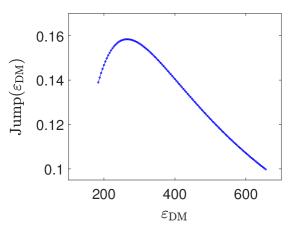
(a) Identifying the value $\varepsilon_{\hbox{{\ppcarac o}}}$ of $\varepsilon_{\hbox{{\pppppcarac DM}}}$

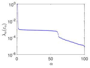
(b) Eigenvalues of the transition matrix

Figure 2: Diffusion map basis of the standard PLoM (No group).

The PLoM algorithm with no group is then used for generating the learned set $\{{\boldsymbol{\eta}}_{\hbox{{\pppcarac ar}}}^{\ell},\ell=1,\ldots,N_{\hbox{{\pppcarac ar}}}\}$. Figure 3 shows the pdf of each one of the random variables $H_{4}$, $H_{5}$, $H_{6}$, and $H_{7}$ estimated with the learned set. Each pdf is estimated (i) with the $N$ realizations of the training set, (ii) with the $N_{\hbox{{\pppcarac ref}}}$ realizations of the reference data set, (iii) with the $N_{\hbox{{\pppcarac ar}}}$ additional realizations generated with the Hamiltonian MCMC algorithm corresponding to the PLoM with $m_{\hbox{{\ppcarac o}}}=N$ and $[g_{m_{\hbox{{\ppppcarac o}}}}]=[I_{N}]$, and referenced as ”No-PLoM”, and finally, with the $N_{\hbox{{\pppcarac ar}}}$ realizations of the learned set constructed with the PLoM for which the partition in groups is not taken into account and referenced as ”No-Group PLoM” (in this case no constraints are applied). It can be seen that the No-PLoM estimation yields a big scattering with an important increase of the dispersion (and thus a loss of the concentration of the probability measure) while No-Group PLoM preserves the concentration of the probability measure (as expected) and the pdfs’ estimations are good enough. These estimations will be improved by using the PLoM with groups and referenced as ”With-Group PLoM”.

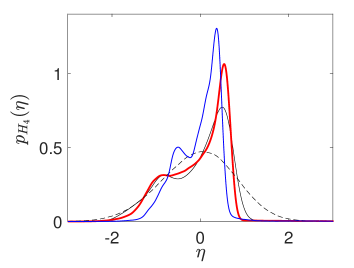
(a) pdf of $H_{4}$

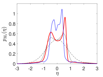
(b) pdf of $H_{5}$

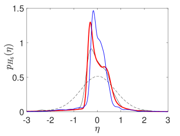
(c) pdf of $H_{6}$

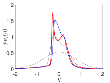
(d) pdf of $H_{7}$

Figure 3: pdf estimated with (i) the training set (black thin), (ii) the reference data set (red thick), (iii) No-PLoM (dashed) , and (iv) No-Group PLoM (blue thin).

3.2 Computing the partition

The optimal partition is computed as explained in Section 2.4.1. Figure 4a displays the graph of $i_{\hbox{{\pppcarac ref}}}\mapsto\tau(i_{\hbox{{\pppcarac ref}}})$, which shows that $i_{\hbox{{\pppcarac ref}}}^{\,{\hbox{{\ppcarac o}}}}=0.013$. Finally, the algorithm identifies the partition and finds $n_{p}=3$ groups with $\nu_{1}=10$, $\nu_{2}=20$, and $\nu_{3}=30$ and with ${\textbf{Y}}^{1}=(H_{1},\ldots,H_{10})$, ${\textbf{Y}}^{2}=(H_{11},\ldots,H_{30})$, and ${\textbf{Y}}^{3}=(H_{31},\ldots,$ $H_{60})$, which correspond to the model introduced in Appendix A for generating the training set. This result constitutes an additional validation of the optimal partition algorithm that is used for non-Gaussian random vectors. For illustration, Figure 4b displays the graph of the joint pdf of random variables $H_{1}$ and $H_{2}$.

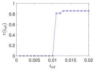
(a) Graph of function $i_{\hbox{{\pppcarac ref}}}\mapsto\tau(i_{\hbox{{\pppcarac ref}}})$

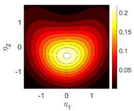
(b) Joint pdf of $H_{1}$ and $H_{2}$

Figure 4: Partition of H in $n_{p}$ mutually independent random vectors ${\textbf{Y}}^{1},\ldots,{\textbf{Y}}^{n_{p}}$.

3.3 PLoM analysis with groups (With-Group PLoM)

Algorithm 1 is used for each group $i=1,2,3$. We then have $m_{i,{\hbox{{\ppcarac o}}}}=\nu_{i}+1$. The training set $\{{\boldsymbol{\eta}}_{d}^{i,j},j=1,\ldots,N\}$ of ${\textbf{Y}}^{i}$ is used. A similar graph to the one shown in Figure 2a is constructed for identifying the optimal value $\varepsilon_{i,{\hbox{{\ppcarac o}}}}$ of the smoothing parameter $\varepsilon_{i,{\hbox{{\pppppcarac DM}}}}$ yielding $\varepsilon_{1,{\hbox{{\ppcarac o}}}}=412$, $\varepsilon_{2,{\hbox{{\ppcarac o}}}}=896$, and $\varepsilon_{3,{\hbox{{\ppcarac o}}}}=1\,132$. Figure 5a shows the distribution of the eigenvalues of the transition matrix of each group $i$ computed for $\varepsilon_{i,{\hbox{{\pppppcarac DM}}}}=\varepsilon_{i,{\hbox{{\ppcarac o}}}}$. It can be seen that all the required criteria are satisfied.

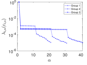
(a) Eigenvalues of the transition matrix of group $i$ computed for $\varepsilon_{i,{\hbox{{\pppppcarac DM}}}}=\varepsilon_{i,{\hbox{{\ppcarac o}}}}$

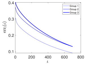
(b) Error function $\iota\mapsto{\hbox{{\ppcarac err}}}_{i}(\iota)$ of group $i$ for iteration number $\iota$ of the iteration algorithm

Figure 5: Diffusion map basis and error function of the iteration algorithm for each one of the $3$ groups, $i=1,2,3$.

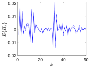
(a) Mean value of $H_{k}$

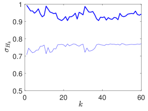
(b) Standard deviation of $H_{k}$

Figure 6: Mean value and standard deviation of the components $H_{k}$, $k=1,\ldots,\nu$, of H estimated using the learned set generated by No-Group PLoM (thin line) and by With-Group PLoM (thick line).

For each group $i=1,2,3$, the PLoM method with groups is used for generating the learned set $\{{\boldsymbol{\eta}}_{\hbox{{\pppcarac ar}}}^{i,j},j=1,\ldots,N_{\hbox{{\pppcarac ar}}}\}$. The constraints $E\{(Y^{i}_{k})^{2}\}=1$ for $k\in\{1,\ldots,\nu_{i}\}$ are applied and the iterative algorithm introduced in Section 2.4.4 is used. Figure 5b displays the error function $\iota\mapsto{\hbox{{\pcarac err}}}_{i}(\iota)$ of group $i$, defined by Eq. (6), which shows the convergence of the iterative algorithm. It should be noted that the convergence could have been pushed further, but the numerical experiments showed that the additional gain obtained is negligible. In addition, numerical experiments have been carried out to compare the efficiency of the type of constraints. We have verified that taking into account all the constraints (mean of ${\textbf{Y}}^{i}$ equal to 0 and covariance matrix $[C_{{\textbf{Y}}^{i}}]=[I_{\nu_{i}}]$) did not provide significant improvements on the preservation of the concentration of the probability measure compared to the sole application of the constraints $E\{(Y^{i}_{k})^{2}\}=1$ for $k\in\{1,\ldots,\nu_{i}\}$. Figure 6 shows the mean value and the standard deviation of the components $H_{k}$, $k=1,\ldots,\nu$ of H estimated using the learned set generated by No-Group PLoM (see Section 3.1) and by With-Group PLoM. Figure 6a shows that the mean values are reasonably small with respect to $1$ and therefore that it is not necessary to improve it by introducing the constraints for the mean. Figure 6b shows that the standard deviations are improved by using With-Group PLoM for which the constraints are taken into account. Figure 7 shows the pdf of $H_{4}$, $H_{5}$, $H_{6}$, and $H_{7}$ estimated with the learned set. Similarly to Section 3.3, each pdf is estimated (i) with the $N$ realizations of the training set, (ii) with the $N_{\hbox{{\pppcarac ref}}}$ realizations of the reference data set, (iii) with the $N_{\hbox{{\pppcarac ar}}}$ additional realizations computed by No-PLoM, and (iv) with the $N_{\hbox{{\pppcarac ar}}}$ realizations computed by With-Group PLoM. Comparing Figure 3 with Figure 7, it can be seen that the use of groups improves the pdfs’ estimations as expected. It can also be noted that the estimates are excellent for this very difficult case in particular by comparing with the usual approach (see the dashed lines corresponding to No-PLoM).

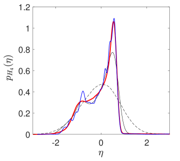
(a) pdf of $H_{4}$

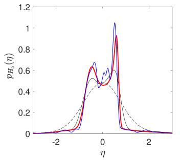
(b) pdf of $H_{5}$

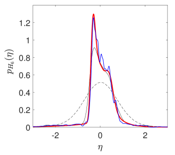
(c) pdf of $H_{6}$

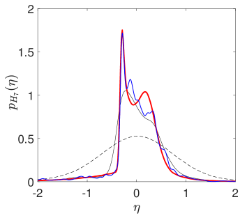
(d) pdf of $H_{7}$

Figure 7: pdf estimated with (i) the training set (black thin), (ii) the reference data set (red thick), (iii) No-PLoM (dashed) , and (iv) With-Group PLoM (blue thin).

3.4 Quantifying the concentration of the probability measure

For No PLoM, the computations are performed as explained in Section 3.1, for No-Group PLoM as in Sections 2.3 and 3.1, and for With-Group PLoM as in Sections 3.3 and 2.4.

(i) The results concerning the concentration of the probability measure are summarized in Table 1. For No PLoM, $d^{2}_{N}(N)$ is computed with Eq. (4) for which $m=N=1\,200$. For No-Group PLoM, $d^{2}_{N}(m_{\hbox{{\ppcarac o}}})$ is also computed with Eq. (4) but with $m=m_{\hbox{{\ppcarac o}}}=61$. For With-Group PLoM, $d^{2}_{wg,N}({\textbf{m}}_{\hbox{{\ppcarac o}}})$ is computed with Eq. (7) for which ${\textbf{m}}_{\hbox{{\ppcarac o}}}=(m_{1,{\hbox{{\ppcarac o}}}},m_{2,{\hbox{{\ppcarac o}}}},m_{3,{\hbox{{\ppcarac o}}}})$ with $m_{1,{\hbox{{\ppcarac o}}}}=11$, $m_{2,{\hbox{{\ppcarac o}}}}=21$, and $m_{3,{\hbox{{\ppcarac o}}}}=31$, and where $d^{2}_{i,N}(m_{i,{\hbox{{\ppcarac o}}}})$ are computed using Eq. (8), which yields $d^{2}_{1,N}(m_{1,{\hbox{{\ppcarac o}}}})=0.012$, $d^{2}_{2,N}(m_{2,{\hbox{{\ppcarac o}}}})=0.015$, and $d^{2}_{3,N}(m_{3,{\hbox{{\ppcarac o}}}})=0.019$. The results obtained are those that were hoped for. Without using the PLoM method, we find numerically $d^{2}_{N}(N)\simeq 2$ that is the theoretical value (see Section 2.3.5). We also see that $d^{2}_{N}(m_{\hbox{{\ppcarac o}}})=0.094\ll 2$, which shows that the usual PLoM method (without group) effectively preserves the concentration of the probability measure unlike the usual MCMC method that does not allow it. For the PLoM with groups, an improvement is observed relative to the PLoM without group as indicated by the evaluation $d^{2}_{wg,N}({\textbf{m}}_{\hbox{{\ppcarac o}}})=0.016\ll d^{2}_{N}(m_{\hbox{{\ppcarac o}}})=0.094$. The quantification of the probability of the random relative distance defined by Eq. (12) confirms this improvement. Note that the probability $(r/\varepsilon)^{n_{p}}$ corresponds to an upper value, the probability being certainly smaller.

Table 1: Concentration of the probability measure for Application 1

No	PLoM	PLoM
PLoM	No Group	With Group
	$m_{\hbox{{\ppcarac o}}}=61$		$\rm{Proba}$ by Eq. (12)
$d^{2}_{N}(N)$	$d^{2}_{N}(m_{\hbox{{\ppcarac o}}})$	$d^{2}_{wg,N}({\textbf{m}}_{\hbox{{\ppcarac o}}})$	$\varepsilon$	$\leq(\frac{r}{\varepsilon})^{n_{p}}$
$2.00$	$0.094$	$0.016$	$0.05$	$\leq 0.028$
			$0.10$	$\leq 0.0034$

(ii) Concerning the visualization of the concentration of the probability measure, Figure 8 shows the clouds of points $\{\eta_{\hbox{{\pppcarac ar}}}^{\ell},\ell=1,\ldots,N_{\hbox{{\pppcarac ar}}}\}$ for the components $(H_{1},H_{2},H_{3})$, generated (a) without using PLoM (No-PLoM), (b) using the PLoM method without group (No-Group PLoM), and (c) using the PLoM method with groups (With-Group PLoM). The three figures confirm the analysis presented in point (i) above.

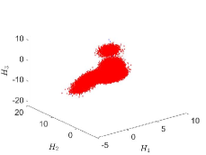
(a) No PLoM

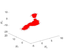
(b) No-Group PLoM

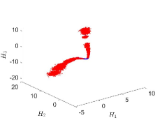
(c) With-Group PLoM

Figure 8: Clouds of the $N_{\hbox{{\pppcarac ar}}}=1\,200\,000$ realizations of $(H_{1},H_{2},H_{3})$ computed with No-PLoM, No-Group PLoM, and With-Group PLoM.

4 Application 2

The second application is devoted to a supervised learning problem ${\textbf{Q}}={\textbf{f}}({\textbf{W}},{\textbf{U}})$ (see Section 2.1) in high dimension, for which the uncontrolled random parameter is the ${\mathbb{R}}^{n_{u}}$-valued random variable U with $n_{u}=420\,000$, the random control random parameter is the ${\mathbb{R}}^{n_{w}}$-valued random variable W with $n_{w}=2$, and the QoI is the ${\mathbb{R}}^{n_{q}}$-valued random variable Q with $n_{q}=10\,098$.

4.1 Generation of the training set and reference data set

This application relates to a linear elastic system modeled by an elliptic stochastic boundary problem (BVP) in a 3D bounded domain $\Omega$, described in the SI Units. The generic point of $\Omega$ is ${\boldsymbol{\zeta}}=(\zeta_{1},\zeta_{2},\zeta_{3})$ in an orthonormal Cartesian coordinate system $(O,\zeta_{1},\zeta_{2},\zeta_{3})$ with $O=(0,0,0)$. The outward unit normal to $\partial\Omega=\Gamma_{0}\cup\Gamma$ is denoted by ${\textbf{n}}({\boldsymbol{\zeta}})$. There is a zero Dirichlet condition on $\Gamma_{0}$ and a Neumann condition on $\Gamma$. Domain $\Omega$ is occupied by a random linear elastic medium (heterogeneous material). The uncontrolled parameter of the system is the fourth-order tensor-valued non-Gaussian elasticity random field $\{{\mathbb{K}}=\{{\mathbb{K}}_{ijkh}({\boldsymbol{\zeta}})\}_{1\leq i,j,k,h\leq 3},{\boldsymbol{\zeta}}\in\Omega\}$ (random coefficients of the partial differential operator) for which the mean value is isotropic and the statistical fluctuations are anisotropic. The control parameter ${\textbf{w}}=(w_{1},w_{2})$ of the system consists of $w_{1}=\log(L_{\hbox{{\ppppcarac corr}}})$ in which $L_{\hbox{{\ppppcarac corr}}}$ is a spatial correlation length and of $w_{2}=\log(\delta_{G})$ in which $\delta_{G}$ is a dispersion parameter, which allow the statistical fluctuations of ${\mathbb{K}}$ to be controlled. The observation of the system is the ${\mathbb{R}}^{3}$-valued random displacement field ${\textbf{V}}=(V_{1},V_{2},V_{3})$ on $\Omega$, which is the random solution of the stochastic BVP,

$$-\hbox{{\Ppcarac div}}\,\,{{\boldsymbol{\Sigma}}} ={\hbox{\bf 0}}\quad\hbox{in}\quad\Omega\,,$$

V $$={\hbox{\bf 0}}\quad\hbox{on}\quad\Gamma_{0}\,,$$

$${\boldsymbol{\Sigma}}\,{\textbf{n}} ={\boldsymbol{{\mathcal{G}}}}^{\Gamma}\quad\hbox{on}\quad\Gamma\,.$$

The stress tensor ${\boldsymbol{\Sigma}}=\{\Sigma_{ij}\}_{1\leq i,j\leq 3}$ is related to the strain tensor ${\textbf{E}}({\textbf{V}})=\{E_{kh}({\textbf{V}})\}_{1\leq k,h\leq 3}$ by the constitutive equation, $\Sigma_{ij}({\boldsymbol{\zeta}})={\mathbb{K}}_{ijkh}({\boldsymbol{\zeta}})\,E_{kh}({\textbf{V}}({\boldsymbol{\zeta}}))$ in which the strain tensor is such that $E_{kh}({\textbf{V}})=(\partial V_{k}/\partial\zeta_{h}+\partial V_{h}/\partial\zeta_{k})/2$. The geometry, the surface force field ${\boldsymbol{{\mathcal{G}}}}^{\Gamma}$, the probabilistic model of the elasticity random field ${\mathbb{K}}$ that depends on parameter w, and the finite element discretization of the weak formulation of the stochastic BVP are detailed in Appendix B.

The control parameter w is modelled by a ${\mathbb{R}}^{2}$-valued random variable ${\textbf{W}}=(W_{1},W_{2})$. The random vectors U, W, and Q, for which the dimensions are $n_{u}=420\,000$, $n_{w}=2$, and $n_{q}=10\,098$, are defined in Appendix B. The random vectors W and U are statistically independent. The dimension $n=n_{q}+n_{w}$ of random vector ${\textbf{X}}=({\textbf{Q}},{\textbf{W}})$ is thus $n=10\,000$.

The training set is generated as explained in Section 2.1 for which $N=100$ independent realizations, ${\textbf{u}}_{d}^{j}$ and ${\textbf{w}}_{d}^{j}$, of U and W are generated using the probabilistic model detailed in Appendix B. For each $j\in\{1,\ldots,N\}$, the realization ${\textbf{q}}_{d}^{j}$ of Q is computed by solving the BVP using the computational model (finite element discretization of the BVP), which is such that ${\textbf{q}}_{d}^{j}={\textbf{f}}({\textbf{w}}_{d}^{j},{\textbf{u}}_{d}^{j})$ (note that f is not explicitly known and results from the solution of the BVP). The training set related to random vector ${\textbf{X}}=({\textbf{Q}},{\textbf{W}})$ is then made up of the $N$ independent realizations $\{{\textbf{x}}_{d}^{j},j=1,\ldots,N\}$ in which ${\textbf{x}}_{d}^{j}=({\textbf{q}}_{d}^{j},{\textbf{w}}_{d}^{j})\in{\mathbb{R}}^{n}$.

The reference data set $\{{\textbf{x}}_{\hbox{{\pppcarac ref}}}^{\ell},\ell=1,\ldots,N_{\hbox{{\pppcarac ref}}}\}$ for X is generated as the training set but with $N_{\hbox{{\pppcarac ref}}}=20\,000$ independent realizations. Computations have been made for $N_{\hbox{{\pppcarac ref}}}=15\,000$, $18\,000$, and $20\,000$, which have shown that the pdf of each observed component of Q were converged for $N_{\hbox{{\pppcarac ref}}}=20\,000$ (note that the construction of the reference has been very CPU time consuming).

The learned sets generated without using the PLoM method (No PLoM), or using the PLoM method with no group (No-Group PLoM), or with groups (With-Group PLoM) will be all performed with $N_{\hbox{{\pppcarac ar}}}=200\,000$ realizations $\{{\boldsymbol{\eta}}_{\hbox{{\pppcarac ar}}}^{\ell},\ell=1,\ldots,N_{\hbox{{\pppcarac ar}}}\}$ ($N_{\hbox{{\pppcarac ar}}}=n_{\hbox{{\ppppcarac MC}}}\times N$ with $n_{\hbox{{\ppppcarac MC}}}=2\,000$).

4.2 PLoM analysis without and with partition

In this section, we give the main results without too many details (paper length limitation), knowing that we have already presented a detailed analysis for Application 1.

(i) PCA of random vector X

Since $n=10\,000\ll N=100$, the eigenvalue problem of $[C_{\textbf{X}}]$ is solved using a thin SVD of matrix $[x_{d}]=[{\textbf{x}}_{d}^{1}\ldots{\textbf{x}}_{d}^{N}]\in{\mathbb{M}}_{n,N}$, which thus does not require the assembling of $[C_{\textbf{X}}]$ (as explained in Section 2.2). Figure 9a shows the distribution of the eigenvalues $\mu_{\alpha}$. For constructing the PCA representation, ${\textbf{X}}^{\nu}=\underline{{\textbf{x}}}_{d}+[\Phi]\,[\mu]^{1/2}\,{\textbf{H}}$, of X, we have chosen $\varepsilon_{\hbox{{\ppppcarac PCA}}}=0.001$ that yields $\nu=27$. Following Section 2.2, the matrix $[\eta_{d}]\in{\mathbb{M}}_{\nu,N}$ is constructed with the $\nu$ realizations ${\boldsymbol{\eta}}^{1}_{d},\ldots,{\boldsymbol{\eta}}^{N}_{d}$ of the ${\mathbb{R}}^{\nu}$-valued random variable H.

(ii) Reduced-order diffusion-map basis for No-Group PLoM

Algorithm 1 is used for the calculation of the reduced-order diffusion-map basis $[g_{m_{\hbox{{\ppppcarac o}}}}]$ of the ${\mathbb{R}}^{\nu}$-valued random variable H. For the optimal values $m_{\hbox{{\ppcarac o}}}=\nu+1=28$ and $\varepsilon_{\hbox{{\ppcarac o}}}=103$, Figure 9b shows the eigenvalues $\lambda_{\alpha}$ of the transition matrix.

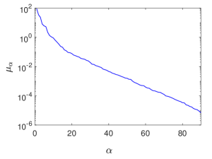
(a) Eigenvalues of the covariance matrix of X

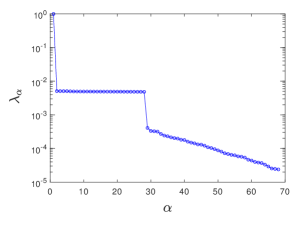
(b) Eigenvalues of the transition matrix

Figure 9: PCA eigenvalues and diffusion map eigenvalues of the PLoM without group (No-Group PLoM).

(iii) Construction of the optimal partition of H

The optimal partition is computed as explained in Section 2.4.1. Figure 10a displays the graph of $i_{\hbox{{\pppcarac ref}}}\mapsto\tau(i_{\hbox{{\pppcarac ref}}})$, which shows that $i_{\hbox{{\pppcarac ref}}}^{\,{\hbox{{\ppcarac o}}}}=0.112$. The algorithm identifies the partition and finds $n_{p}=9$ groups such that $\nu_{1}=5$ with ${\textbf{Y}}^{1}=(H_{1},H_{2},H_{4},H_{16},H_{19})$, $\nu_{2}=1$ with $Y^{2}=H_{3}$, $\nu_{3}=15$ with ${\textbf{Y}}^{3}=(H_{5}\,\hbox{to}\,H_{11},H_{14},H_{15},H_{17},H_{18},H_{20},H_{24}\,\hbox{to}\,H_{26}$), and $\nu_{4}=\ldots=\nu_{9}=1$ with $Y^{4}=H_{12}$, $Y^{5}=H_{13}$, $Y^{6}=H_{21}$, $Y^{7}=H_{22}$, $Y^{8}=H_{23}$, and $Y^{9}=H_{27}$. For each one of the two groups $i=1$ and $3$ (having a length greater than $1$), the optimal values are $m_{1,{\hbox{{\ppcarac o}}}}=6$, $m_{3,{\hbox{{\ppcarac o}}}}=16$, $\varepsilon_{1,{\hbox{{\ppcarac o}}}}=37.7$, and $\varepsilon_{3,{\hbox{{\ppcarac o}}}}=103$. For these optimal values of $\varepsilon_{i,{\hbox{{\ppcarac o}}}}$, Figure 10b shows the distribution of eigenvalues $\lambda_{i,\alpha}$ of the transition matrix. For the groups $i\neq 1$ and $3$, we have $m_{i,{\hbox{{\ppcarac o}}}}=N$ (see Algorithm 1).

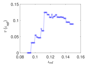
(a) Graph of function $i_{\hbox{{\pppcarac ref}}}\mapsto\tau(i_{\hbox{{\pppcarac ref}}})$

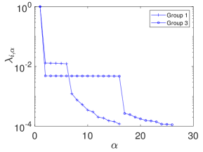
(b) Eigenvalues of the transition matrix

Figure 10: Partition of H in $n_{p}=9$ mutually independent random vectors ${\textbf{Y}}^{1},\ldots,{\textbf{Y}}^{n_{p}}$ and diffusion map eigenvalues of the PLoM for groups $1$ and $3$.

(iv) Influence of the constraints of all the components of ${\textbf{Y}}^{i}$

No-Group PLoM is performed without any constraints applied to random vector H. With-Group PLoM is performed, group by group, in applying, for $i=1,\ldots,n_{p}=9$, the constraints $E\{(Y^{i}_{k})^{2}\}=1$ for $k\in\{1,\ldots,\nu_{i}\}$. For all the components $k=1,\ldots,\nu=27$ of H, Figure 11 shows the mean value $E\{H_{k}\}$ and the standard deviation $\sigma_{H_{k}}$ that are estimated by No-Group PLoM and by With-Group PLoM. We can see that the mean values remain much lower than $1$ although no constraint is applied to the mean, as well for No-Group PLoM as for With-Group PLoM. We can also see that the standard deviation of the components are already close to $1$ for No-Group PLoM although no constraint is applied to the second-order moments. As expected, for With-Group PLoM for which the constraints are applied to the second-order moments, the standard deviations are almost equal to $1$.

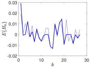
(a) Mean value of $H_{k}$

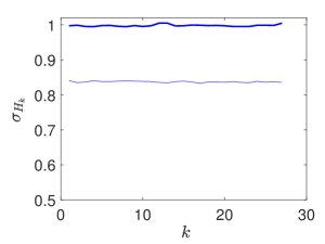
(b) Standard deviation of $H_{k}$

Figure 11: Mean value and standard deviation of the components $H_{k}$, $k=1,\ldots,\nu$, of H estimated using the learned set generated with No-Group PLoM (thin line) and With-Group PLoM (thick line).

(v) pdf of observations estimated by the PLoM

The pdf of components $Q_{17}$ and $Q_{7740}$ of Q are presented in Figure 12. Component $17$ corresponds to the $\zeta_{2}$-axis displacement $V_{2}({\boldsymbol{\zeta}})$ at point ${\boldsymbol{\zeta}}=(0,0,0.1)$ while component $7740$ corresponds to the $\zeta_{3}$-axis displacement $V_{3}({\boldsymbol{\zeta}})$ at point ${\boldsymbol{\zeta}}=(0.78,0,0.1)$.

(a) pdf of $Q_{17}$

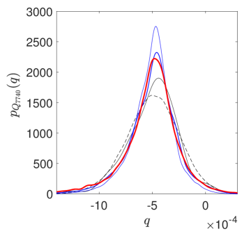
(b) pdf of $Q_{7740}$

Figure 12: pdf estimated with (i) the training dataset (black thin), (ii) the reference dataset (red thick), (iii) No-PLoM (dashed), (iv) No-Group PLoM (blue thin), and (v) With-Group PLoM (blue thick).

Figure 12 shows the pdf estimated (i) with the $N_{d}=100$ points of the training set, (ii) with the $N_{\hbox{{\pppcarac ref}}}=20\,000$ points of the reference data set, (iii) with $N_{\hbox{{\pppcarac ar}}}=200\,000$ additional realizations generated with an usual MCMC generator (without using the PLoM method), (iv) with the $N_{\hbox{{\pppcarac ar}}}=200\,000$ additional realizations of the learned set generated by No-Group PLoM, and finally, (v) with the $N_{\hbox{{\pppcarac ar}}}=200\,000$ additional realizations of the learned set generated by With-Group PLoM for which a partition in $n_{p}=9$ groups has been identified. It can be seen that the usual MCMC method (no PLoM) is not good at all, that No-Group PLoM already gives a good estimation in comparison with the reference, and finally, that With-Group PLoM gives an excellent estimation when compared to the reference.

(vi) Quantifying the concentration of the probability measure

The analysis is carried out as in Section 3.4. The results concerning the concentration of the probability measure is summarized in Table 2 and in Figure 13.

Table 2: Concentration of the probability measure for Application 2

No	PLoM	PLoM
PLoM	No Group	With Group
	$m_{\hbox{{\ppcarac o}}}=28$		$\rm{Proba}$ by Eq. (12)
$d^{2}_{N}(N)$	$d^{2}_{N}(m_{\hbox{{\ppcarac o}}})$	$d^{2}_{wg,N}({\textbf{m}}_{\hbox{{\ppcarac o}}})$	$\varepsilon$	$\leq(\frac{r}{\varepsilon})^{n_{p}}$
$2.00$	$0.16$	$0.044$	$0.05$	$\leq 4.3\times 10^{-5}$
			$0.1$	$\leq 8.3\times 10^{-8}$

For No PLoM, $d^{2}_{N}(N)$ is computed with Eq. (4) for which $m=N=100$. For No-Group PLoM, $d^{2}_{N}(m_{\hbox{{\ppcarac o}}})$ is also computed with Eq. (4) but with $m=m_{\hbox{{\ppcarac o}}}=28$. For With-Group PLoM, $d^{2}_{wg,N}({\textbf{m}}_{\hbox{{\ppcarac o}}})$ is computed with Eq. (7) for which ${\textbf{m}}_{\hbox{{\ppcarac o}}}=(m_{1,{\hbox{{\ppcarac o}}}},\ldots,m_{9,{\hbox{{\ppcarac o}}}})$. The graph $i\mapsto d^{2}_{i,N}(m_{i,{\hbox{{\ppppcarac o}}}})$ is computed using Eq. (8) and is plotted in Figure 13. Without using the PLoM method, we find numerically $d^{2}_{N}(N)=2$ that is the theoretical value (see Section 2.3.5). We also see that $d^{2}_{N}(m_{\hbox{{\ppcarac o}}})=0.16\ll 2$, which shows that the usual PLoM method (without group) effectively preserves the concentration of the probability measure unlike the usual MCMC methods that do not allow it. For the PLoM with groups, it can be seen an improvement with respect to the PLoM without group because $d^{2}_{wg,N}({\textbf{m}}_{\hbox{{\ppcarac o}}})=0.044\ll d^{2}_{N}(m_{\hbox{{\ppcarac o}}})=0.16$. The quantification of the probability of the random relative distance defined by Eq. (12) confirms this improvement. Note that the probability $(r/\varepsilon)^{n_{p}}$ corresponds to an upper value, the probability being certainly smaller.

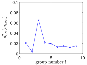
Figure 13: Concentration of the probability measure for each group $i\in\{1,\ldots,9\}$: graph of $i\mapsto d^{2}_{i,N}(m_{i,{\hbox{{\ppppcarac o}}}})$ computed using Eq. (8).

5 Discussion and conclusion

The implementation of a partition in the PLoM method has provided an opportunity to revisit, improve the efficiency, and simplify the algorithm to identify the optimal values of the hyperparameters of the reduced-order diffusion-map basis. This was made necessary for the PLoM method with partition, because the number of groups identified can be large and for each group of dimension greater than 1, the reduced-order diffusion-map basis must be constructed. This new efficient algorithm is common to PLoM with or without partition.

Still within the framework of the PLoM carried out with partition, we have made the following observations. If a group of the partition has a relatively small dimension (a few units, or even one or two dozen) and if the support of its probability measure has a complex geometry, one could obtain a significant loss of normalization compared to 1 (for instance 0.6 or 0.7 instead of 0.9 or 1). For instance, such a situation can be encountered by the presence of numerous non-Gaussian stochastic germs that generate strong statistical fluctuations (for example, up to ten times the standard deviation for some components). For these cases, we have proposed to introduce constraints on the second-order moments of the components of such a group, by reusing the Kullback-Leibler minimum cross-entropy principle that we have previously used for taking into account physics constraints in the PLoM method. For instance, Application 1 is very difficult due to the high degree of the polynomials in the model; although the realizations of the training set are centered and have a covariance matrix equal to the identity matrix, the fluctuations vary between $-10$ and +$10$ for some components (which must be compared to a magnitude of $1$). It should be noted that we have also developed, tested, and implemented the general case of introducing constraints on the mean vector (zero mean) and on the covariance matrix (identity matrix). One then increases considerably the number of Lagrange multipliers to be calculated by the iterative method, which induces a significant numerical additional cost. We have not seen any significant improvement compared to the only constraint related to the diagonal of the covariance matrix (second-order moments equal to $1$ knowing that the centering is reasonably well obtained without constraint on the mean vector). Under these conditions we have only presented the simplest case of constraints and we have demonstrated it on two applications.

In the recently published mathematical foundations of PLoM [5], to establish the main theorem, we introduced a distance between the random matrix defined by PLoM and the deterministic matrix that represent all the given points of the training set. In the present paper, and in order to facilitate the quantification of the preservation of the concentration of the probability measure between the usual MCMC method (No PLoM), the PLoM method without partition (No-Group PLoM), and the PLoM method with partition (With-Group PLoM), we apply this distance to each group of the partition. We have assessed it numerically for the two applications. The results obtained confirm the theoretical results: there is a significant loss of concentration of the probability measure for the usual MCMC method (No PLoM) while the PLoM method without partition (No-Group PLoM) preserves well the concentration of the probability measure. In addition, this distance shows that the PLoM method with partition further improves the preservation of the concentration of the probability measure compared to the PLoM method without partition, which was hoped for. Finally, to complete the quantification of the concentration of the probability measure by the distance, we have also proven a mathematical result of this quantification in terms of probability. This result shows that if the number of groups of the partition increases, then the gain of With-Group PLoM can be significantly improved compared to No-Group PLoM. We have numerically quantified these probabilities for the two applications.

This work contributes to the improvement of the PLoM method. The results presented are very satisfactory for the two applications which, while quite distinct, present significant challenges to other statistical learning methods.

Appendix A Probabilistic model of the random generator for Applications 1

In this Appendix, any second-order random quantity S is defined on a probability space $(\Theta,{\mathcal{T}},{\mathcal{P}})$ and its mathematical expectation $E\{{\textbf{S}}\}$ is estimated by $\underline{{\textbf{s}}}=(1/N)\sum_{j=1}^{N}{\textbf{s}}^{j}$ using $N$ independent realizations $\{{\textbf{s}}^{j}={\textbf{S}}(\theta_{j}),j=1,\ldots,N\}$ of S with $\theta_{j}\in\Theta$.

The ${\mathbb{R}}^{\nu}$-valued random variable ${\textbf{H}}=(H_{1},\ldots,H_{\nu})$ is written as a partition of $n_{p}=3$ independent random vectors ${\textbf{Y}}^{1},\ldots,{\textbf{Y}}^{n_{p}}$ such that, for $i=1,\ldots,n_{p}$, the normalized ${\mathbb{R}}^{\nu_{i}}$-valued random variable ${\textbf{Y}}^{i}=(Y^{i}_{1},\ldots,Y^{i}_{\nu_{i}})$ is non-Gaussian and such that the estimate of its mean vector is $\underline{{\boldsymbol{\eta}}^{i}}={\hbox{\bf 0}}_{\nu_{i}}$ and the estimate of its covariance matrix is $[C_{{\textbf{Y}}^{i}}]=[I_{\nu_{i}}]$. We have $\nu=\nu_{1}+\ldots+\nu_{n_{p}}$ and we choose $\nu_{1}=10$, $\nu_{2}=20$, and $\nu_{3}=30$.

For $i=1,2,3$, let $[\,b^{i}]$ be the deterministic matrix in ${\mathbb{M}}_{\nu_{i}}$ defined by: $rng(^{\prime}default^{\prime})$; $[\,b^{i}]=(0.15\times rand(\nu_{i},\nu_{i})+0.85)/\nu_{i}$ (in which $rng$ and $rand$ are the Matlab functions). Let ${\textbf{U}}^{i}=2\,[\,b^{i}]\,{\boldsymbol{{\mathcal{U}}}}^{i}-{\mathonebb{1}}$ be the ${\mathbb{R}}^{\nu_{i}}$-valued random variable in which ${\mathonebb{1}}=(1,\ldots,1)$ and where ${\boldsymbol{{\mathcal{U}}}}^{i}=({\mathcal{U}}^{i}_{1},\ldots,{\mathcal{U}}^{i}_{\nu_{i}})$ is the random vector constituted of $\nu_{i}$ independent uniform random variables on $[0,1]$, whose $N$ independent realizations are $\{{\boldsymbol{{\mathcal{U}}}}^{i}(\theta_{j}),j=1,\ldots,N\}$. The random vectors ${\boldsymbol{{\mathcal{U}}}}^{1}$, ${\boldsymbol{{\mathcal{U}}}}^{2}$, and ${\boldsymbol{{\mathcal{U}}}}^{3}$ are statistically independent. Let ${\boldsymbol{{\mathcal{M}}}}^{i}=({\mathcal{M}}^{i}_{1},\ldots,{\mathcal{M}}^{i}_{\nu_{i}})$ be the ${\mathbb{R}}^{\nu_{i}}$-valued random variable in which, for $k=1,\ldots,\nu_{i}$, ${\mathcal{M}}^{i}_{k}$ is the random monomial ${\mathcal{M}}^{i}_{k}=\sqrt{k!}\,(U^{i}_{k})^{k}$ (thus the degree of this monomial is $k$). Let be ${\boldsymbol{{\mathcal{M}}}}^{i}_{c}={\boldsymbol{{\mathcal{M}}}}^{i}-\underline{{\textbf{m}}^{i}}$ in which $\underline{{\textbf{m}}^{i}}$ is the estimate of the mean value of ${\boldsymbol{{\mathcal{M}}}}^{i}$. Let $[C_{{\boldsymbol{{\mathcal{M}}}}^{i}}]$ be the estimate of the covariance matrix of ${\boldsymbol{{\mathcal{M}}}}^{i}$ and let $[L^{i}]$ be the upper triangular matrix computed from the Cholesky factorization $[C_{{\boldsymbol{{\mathcal{M}}}}^{i}}]=[L^{i}]^{T}\,[L^{i}]$. Therefore, the random vector ${\textbf{Y}}^{i}$ is constructed as ${\textbf{Y}}^{i}=([L^{i}]^{T})^{-1}\,{\boldsymbol{{\mathcal{M}}}}^{i}_{c}$ whose the $N$ independent realizations $\{{\boldsymbol{\eta}}_{d}^{i,j},j=1,\ldots,N\}$ are such that ${\boldsymbol{\eta}}_{d}^{i,j}=([L^{i}]^{T})^{-1}\,{\boldsymbol{{\mathcal{M}}}}^{i}_{c}(\theta_{j})$. The $N$ independent realizations $\{{\boldsymbol{\eta}}_{d}^{j},j=1,\ldots,N\}$ of H are such that ${\boldsymbol{\eta}}_{d}^{j}=({\boldsymbol{\eta}}_{d}^{1,j},{\boldsymbol{\eta}}_{d}^{2,j},{\boldsymbol{\eta}}_{d}^{3,j})\in{\mathbb{R}}^{\nu}={\mathbb{R}}^{\nu_{1}}\times{\mathbb{R}}^{\nu_{2}}\times{\mathbb{R}}^{\nu_{3}}$. Using these $N$ realizations, the estimate of the mean vector of H is $\underline{{\boldsymbol{\eta}}}={\hbox{\bf 0}}_{\nu}$ and the estimate of its covariance matrix is $[C_{{\textbf{H}}}]=[I_{\nu}]$. By construction, we have ${\textbf{Y}}^{1}=(H_{1},\ldots,H_{10})$, ${\textbf{Y}}^{2}=(H_{11},\ldots,H_{30})$, and ${\textbf{Y}}^{3}=(H_{31},\ldots,H_{60})$.

Appendix B Model and data for Applications 2

(i) Geometry and surface force field ${\boldsymbol{{\mathcal{G}}}}^{\Gamma}$

The 3D bounded domain is defined by $\Omega=]0,1.0[\,\times\,]0,0.2[\,\times\,]0,0.1[$. Its boundary is written as $\partial\Omega=\Gamma_{0}\cup\Gamma$ in which $\Gamma=\partial\Omega\backslash\Gamma_{0}$ with $\Gamma_{0}=\{\zeta_{1}=1.0\,,\,0\leq\zeta_{2}\leq 0.2\,,\,0\leq\zeta_{3}\leq 0.1\}$. The surface force field ${\boldsymbol{{\mathcal{G}}}}^{\Gamma}=({\mathcal{G}}^{\Gamma}_{1},{\mathcal{G}}^{\Gamma}_{2},{\mathcal{G}}^{\Gamma}_{3})$ is zero on all $\Gamma$ except on the part $\{\zeta_{1}=0.0\,,\,0\leq\zeta_{2}\leq 0.2\,,\,0\leq\zeta_{3}\leq 0.1\}$ for which ${\mathcal{G}}^{\Gamma}_{1}(\zeta)=-4.95\times 10^{7}\,N/m^{2}$, ${\mathcal{G}}^{\Gamma}_{2}(\zeta)=-4.29\times 10^{5}\,N/m^{2}$, and ${\mathcal{G}}^{\Gamma}_{3}(\zeta)=-1.65\times 10^{5}\,N/m^{2}$.

(ii) Probabilistic modeling of the elasticity random field

Random field ${\mathbb{K}}$ is rewritten as ${\mathbb{K}}_{ijkh}({\boldsymbol{\zeta}})=[{\textbf{K}}({\boldsymbol{\zeta}})]_{IJ}$ with $I=(i,j)$ and $J=(k,h)$, in which indices $I$ and $J$ belong to $\{1,\ldots,6\}$, and where $\{[{\textbf{K}}({\boldsymbol{\zeta}})],{\boldsymbol{\zeta}}\in{\mathbb{R}}^{3}\}$ is a second-order ${\mathbb{M}}_{6}^{+}$-valued non-Gaussian random field indexed by ${\mathbb{R}}^{3}$, which is assumed to be statistically homogeneous. Its mean function $[\underline{K}]\in{\mathbb{M}}_{6}^{+}$ is thus independent of ${\boldsymbol{\zeta}}$ and corresponds to the elasticity tensor of a homogeneous isotropic elastic medium whose Young modulus is $10^{10}\,N/m^{2}$ and Poisson coefficient $0.15$. The statistical fluctuations of random field $[{\textbf{K}}]$ around $[\underline{K}]$ are those of a heterogeneous anisotropic elastic medium. The non-Gaussian ${\mathbb{M}}_{6}^{+}$-valued random field $\{[{\textbf{K}}({\boldsymbol{\zeta}})]\,,{\boldsymbol{\zeta}}\in\Omega\}$ is constructed using the stochastic model [30, 31] of random elasticity fields for heterogeneous anisotropic elastic media that are isotropic in statistical mean and exhibit anisotropic statistical fluctuations. Its parameterization consists of three spatial-correlation lengths, one dispersion parameter, and a positive-definite lower bound. Random field $[{\textbf{K}}]$ is written, for all ${\boldsymbol{\zeta}}$ in ${\mathbb{R}}^{3}$, as $[{\textbf{K}}({\boldsymbol{\zeta}})]=[K_{\ell}]+[\underline{L}_{\varepsilon}]^{T}\,[{{\textbf{G}}_{0}}({\boldsymbol{\zeta}})]\,[\underline{L}_{\varepsilon}]$. The lower-bound matrix is defined by $[K_{\ell}]=\varepsilon(1+\varepsilon)^{-1}\,[\underline{K}]\in{\mathbb{M}}_{6}^{+}$ in which $\varepsilon$ is chosen equal to $10^{-6}$. The upper triangular matrix $[\underline{L}_{\varepsilon}]\in{\mathbb{M}}_{6}$ is written as $[\underline{L}_{\varepsilon}]=(1+\varepsilon)^{-1/2}\,[\underline{L}]$ in which $[\underline{K}]=[\underline{L}]^{T}\,[\underline{L}]$ (Cholesky factorization). The non-Gaussian random field $\{[{{\textbf{G}}_{0}}({\boldsymbol{\zeta}})],{\boldsymbol{\zeta}}\in{\mathbb{R}}^{3}\}$, which is indexed by ${\mathbb{R}}^{3}$ with values in ${\mathbb{M}}_{6}^{+}$, is homogeneous in ${\mathbb{R}}^{3}$ and is a second-order random field whose modeling and generator are detailed Pages 272 to 274 of [31]. For all ${\boldsymbol{\zeta}}$ in ${\mathbb{R}}^{3}$, the random matrix $[{{\textbf{G}}_{0}}({\boldsymbol{\zeta}})]$ is written as $[{\textbf{G}}_{0}({\boldsymbol{\zeta}})]=[{\textbf{L}}_{G}({\boldsymbol{\zeta}})]^{T}\,[{\textbf{L}}_{G}({\boldsymbol{\zeta}})]$ in which $[{\textbf{L}}_{G}({\boldsymbol{\zeta}})]$ is an upper $(6\times 6)$ real triangular random matrix that depends of $n_{G}=21$ independent normalized Gaussian random variables. Random field $[{\textbf{G}}_{0}]$ depends on $3$ spatial correlation lengths, $L_{{\hbox{{\ppppcarac corr}}},1}$, $L_{{\hbox{{\ppppcarac corr}}},2}$, $L_{{\hbox{{\ppppcarac corr}}},3}$, relative to each one of the three directions $\zeta_{1}$-, $\zeta_{2}$-, and $\zeta_{3}$-axes. It also depends on the dispersion parameter $\delta_{G}>0$ that allows for controlling the level of statistical fluctuations. As explained in Section 4.1, only two hyperparameters are kept: $L_{\hbox{{\ppppcarac corr}}}$ and $\delta_{G}$, for which we have chosen $L_{{\hbox{{\ppppcarac corr}}},1}=L_{{\hbox{{\ppppcarac corr}}},2}=L_{{\hbox{{\ppppcarac corr}}},3}=L_{\hbox{{\ppppcarac corr}}}$.

(iii) Finite element approximation of the stochastic boundary value problem and definition of random vector U

Domain $\Omega$ is meshed with $50\!\times\!10\!\times\!5=2\,500$ finite elements using $8$-nodes finite elements. There are $3\,366$ nodes and $10\,098$ dofs (degrees of freedom) before applying the Dirichlet conditions. The displacements are locked at all the $66$ nodes belonging to surface $\Gamma_{0}$ and therefore, there are $198$ zero Dirichlet conditions. There are $8$ integration points in each finite element. Consequently, there are $N_{i}=20\,000$ integration points ${\boldsymbol{\zeta}}^{1},\ldots,{\boldsymbol{\zeta}}^{N_{i}}$. Let us consider the ${\mathbb{R}}^{n_{u}}$-valued random variable U constituted of all the $n_{u}=N_{i}\!\times\!n_{G}=20\,000\!\times\!21=420\,000$ independent normalized Gaussian random variables that allow the set $\{[{\textbf{L}}_{G}({\boldsymbol{\zeta}}^{1})],\ldots,[{\textbf{L}}_{G}({\boldsymbol{\zeta}}^{N_{i}})]\}$ of random matrices to be generated.

(iv) Construction of random vectors Q, and W

The ${\mathbb{R}}^{n_{q}}$-valued random variable Q of the QoIs are constituted of the $10\,098$ dofs of the discretization of the random displacement field V. The random vector ${\textbf{W}}=(W_{1},W_{2})$ in such that $W_{1}=\log(L_{\hbox{{\ppppcarac corr}}})$ and $W_{2}=log(\delta_{G})$. The random variables $L_{\hbox{{\ppppcarac corr}}}$ and $\delta_{G}$ are independent and uniform on $[0.1\,,1.0]$ and $[0.1\,0.5]$, respectively. We then have $L_{\hbox{{\ppppcarac corr}}}=0.9\,{\mathcal{U}}_{1}+0.1$ and $\delta_{G}=0.4\,{\mathcal{U}}_{2}+0.1$ in which ${\mathcal{U}}_{1}$ and ${\mathcal{U}}_{2}$ are two independent uniform random variable on $[0\,,1]$.

References

- [1] C. Soize, R. Ghanem, Data-driven probability concentration and sampling on manifold, Journal of Computational Physics 321 (2016) 242–258. doi:10.1016/j.jcp.2016.05.044.
- [2] R. Ghanem, C. Soize, L. Mehrez, V. Aitharaju, Probabilistic learning and updating of a digital twin for composite material systems, International Journal for Numerical Methods in Engineering (2020). doi:10.1002/nme.6430.
- [3] R. Ghanem, C. Soize, C. Safta, X. Huan, G. Lacaze, J. C. Oefelein, H. N. Najm, Design optimization of a scramjet under uncertainty using probabilistic learning on manifolds, Journal of Computational Physics 399 (2019) 108930. doi:10.1016/j.jcp.2019.108930.
- [4] M. Arnst, C. Soize, K. Bulthies, Computation of sobol indices in global sensitivity analysis from samll data sets by probabilistic learning on manifolds, International Journal for Uncertainty Quantification online, 19 August 2020 (2020). doi:10.1615/Int.J.UncertaintyQuantification.2020032674.
- [5] C. Soize, R. Ghanem, Probabilistic learning on manifolds, Foundations of Data Science (2020) 1–29doi:10.3934/fods.2020013.
- [6] C. Soize, R. Ghanem, C. Desceliers, Sampling of bayesian posteriors with a non-gaussian probabilistic learning on manifolds from a small dataset, Statistics and Computing 30 (5) (2020) 1433–1457. doi:10.1007/s11222-020-09954-6.
- [7] C. Soize, R. Ghanem, Physics-constrained non-gaussian probabilistic learning on manifolds, International Journal for Numerical Methods in Engineering 121 (1) (2020) 110–145. doi:10.1002/nme.6202.
-
[8]
C. Soize, R. Ghanem, Probabilistic
learning on manifolds constrained by nonlinear partial differential equations
for small datasets, arXiv:2010.14324 [stat.ML] (2020) 1–38.
URL http://arxiv.org/abs/2010.14324 - [9] J. L. Fleiss, B. Levin, M. C. Paik, Statistical Methods for Rates and Proportions, john wiley & sons, 2013.
- [10] P. E. Greenwood, M. S. Nikulin, A guide to Chi-Squared Testing, Vol. 280, John Wiley & Sons, 1996.
- [11] K. Pearson, X. on the criterion that a given system of deviations from the probable in the case of a correlated system of variables is such that it can be reasonably supposed to have arisen from random sampling, The London, Edinburgh, and Dublin Philosophical Magazine and Journal of Science, Series 5 50 (302) (1900) 157–175. doi:10.1080/14786440009463897.
- [12] R. Boscolo, H. Pan, V. P. Roychowdhury, Independent component analysis based on nonparametric density estimation, IEEE Transactions on Neural Networks 15 (1) (2004) 55–65. doi:10.1109/TNN.2003.820667.
- [13] P. Comon, Independent component analysis, a new concept?, Signal processing 36 (3) (1994) 287–314. doi:10.1016/0165-1684(94)90029-9.
- [14] P. Comon, C. Jutten, J. Herault, Blind separation of sources, part ii: Problems statement, Signal processing 24 (1) (1991) 11–20. doi:10.1016/0165-1684(91)90080-3.
- [15] J. Herault, C. Jutten, Space or time adaptive signal processing by neural network models, in: AIP conference proceedings, Vol. 151, American Institute of Physics, 1986, pp. 206–211.
- [16] A. Hyvarinen, Fast and robust fixed-point algorithms for independent component analysis, IEEE transactions on Neural Networks 10 (3) (1999) 626–634. doi:10.1109/72.761722.
- [17] A. Hyvärinen, E. Oja, Independent component analysis: algorithms and applications, Neural networks 13 (4-5) (2000) 411–430. doi:10.1016/S0893-6080(00)00026-5.
- [18] C. Jutten, J. Herault, Blind separation of sources, part i: An adaptive algorithm based on neuromimetic architecture, Signal processing 24 (1) (1991) 1–10. doi:10.1016/0165-1684(91)90079-X.
- [19] T.-W. Lee, M. Girolami, A. J. Bell, T. J. Sejnowski, A unifying information-theoretic framework for independent component analysis, Computers & Mathematics with Applications 39 (11) (2000) 1–21. doi:10.1016/S0898-1221(00)00101-2.
- [20] C. Soize, Optimal partition in terms of independent random vectors of any non-gaussian vector defined by a set of realizations, SIAM/ASA Journal on Uncertainty Quantification 5 (1) (2017) 176–211. doi:10.1137/16M1062223.
- [21] G. H. Golub, C. F. Van Loan, Matrix Computations, Second Edition, Johns Hopkins University Press, Baltimore and London, 1993.
- [22] T. Duong, A. Cowling, I. Koch, M. Wand, Feature significance for multivariate kernel density estimation, Computational Statistics & Data Analysis 52 (9) (2008) 4225–4242. doi:10.1016/j.csda.2008.02.035.
- [23] T. Duong, M. L. Hazelton, Cross-validation bandwidth matrices for multivariate kernel density estimation, Scandinavian Journal of Statistics 32 (3) (2005) 485–506. doi:10.1111/j.1467-9469.2005.00445.x.
- [24] M. Filippone, G. Sanguinetti, Approximate inference of the bandwidth in multivariate kernel density estimation, Computational Statistics & Data Analysis 55 (12) (2011) 3104–3122. doi:10.1016/j.csda.2011.05.023.
- [25] N. Zougab, S. Adjabi, C. C. Kokonendji, Bayesian estimation of adaptive bandwidth matrices in multivariate kernel density estimation, Computational Statistics & Data Analysis 75 (2014) 28–38. doi:10.1016/j.csda.2014.02.002.
- [26] A. Bowman, A. Azzalini, Applied Smoothing Techniques for Data Analysis: The Kernel Approach With S-Plus Illustrations, Vol. 18, Oxford University Press, Oxford: Clarendon Press, New York, 1997. doi:10.1007/s001800000033.
- [27] R. Coifman, S. Lafon, Diffusion maps, Applied and Computational Harmonic Analysis 21 (1) (2006) 5–30. doi:10.1016/j.acha.2006.04.006.
- [28] S. Lafon, A. B. Lee, Diffusion maps and coarse-graining: A unified framework for dimensionality reduction, graph partitioning, and data set parameterization, IEEE transactions on pattern analysis and machine intelligence 28 (9) (2006) 1393–1403. doi:10.1109/TPAMI.2006.184.
- [29] R. Neal, MCMC using hamiltonian dynamics, in: S. Brooks, A. Gelman, G. Jones, X.-L. Meng (Eds.), Handbook of Markov Chain Monte Carlo, Chapman and Hall-CRC Press, Boca Raton, 2011, Ch. 5. doi:10.1201/b10905-6.
- [30] C. Soize, Non gaussian positive-definite matrix-valued random fields for elliptic stochastic partial differential operators, Computer Methods in Applied Mechanics and Engineering 195 (1-3) (2006) 26–64. doi:10.1016/j.cma.2004.12.014.
- [31] C. Soize, Uncertainty Quantification. An Accelerated Course with Advanced Applications in Computational Engineering, Springer, New York, 2017. doi:10.1007/978-3-319-54339-0.