Expanding Boundaries of Gap Safe Screening

Abstract

Sparse optimization problems are ubiquitous in many fields such as statistics, signal/image processing and machine learning. This has led to the birth of many iterative algorithms to solve them. A powerful strategy to boost the performance of these algorithms is known as safe screening: it allows the early identification of zero coordinates in the solution, which can then be eliminated to reduce the problem’s size and accelerate convergence. In this work, we extend the existing Gap Safe screening framework by relaxing the global strong-concavity assumption on the dual cost function. Instead, we exploit local regularity properties, that is, strong concavity on well-chosen subsets of the domain. The non-negativity constraint is also integrated to the existing framework. Besides making safe screening possible to a broader class of functions that includes $\beta$-divergences (e.g., the Kullback-Leibler divergence), the proposed approach also improves upon the existing Gap Safe screening rules on previously applicable cases (e.g., logistic regression). The proposed general framework is exemplified by some notable particular cases: logistic function, $\beta=1.5$ and Kullback-Leibler divergences. Finally, we showcase the effectiveness of the proposed screening rules with different solvers (coordinate descent, multiplicative-update and proximal gradient algorithms) and different data sets (binary classification, hyperspectral and count data).

Keywords: Convex optimization, safe screening rules, sparse regression, $\beta$-divergence, non-negativity

1 Introduction

Safe screening rules have proved to be very powerful tools in order to accelerate the resolution of large-scale sparse optimization problems that arise in statistics, machine learning, signal/image inverse problems, pattern recognition, among other fields. The very principle of safe screening is to identify the zero coordinates in the solution before and/or within the course of iterations of any solver. Once identified, these inactive coordinates can be screened out, thus reducing the size of the problem and consequently the computational load of the solver. Hence, should a screening rule allow to screen many coordinates with a low computational overhead, significant speedups can be observed in practice– see for instance El Ghaoui et al. (2012); Bonnefoy et al. (2015); Ndiaye et al. (2017), and Section 5.

A brief tour of existing screening strategies.

Safe screening rules were initially proposed for the Lasso problem (El Ghaoui et al., 2012) and were later extended to some of its variants: group Lasso (Wang et al., 2015a; Bonnefoy et al., 2015), sparse group Lasso (Ndiaye et al., 2016; Wang et al., 2019), non-negative Lasso (Wang et al., 2019), fused Lasso (Wang et al., 2015), and generalized Lasso (Ren et al., 2018). As opposed to correlation-based feature selection techniques (Fan and Lv, 2008; Tibshirani et al., 2011), safe screening strategies are guaranteed to remove only coordinates that do no belong to the solution support. Beyond Lasso, safe screening has also been used for other machine learning problems, such as: binary logistic regression (El Ghaoui et al., 2012; Ndiaye et al., 2017), metric learning (Yoshida et al., 2018), nuclear norm minimization (Zhou and Zhao, 2015) and support vector machine (Ogawa et al., 2013; Wang et al., 2014; Zimmert et al., 2015).

Three main classes of screening rules can be distinguished: 1) Static rules (El Ghaoui et al., 2012; Xiang et al., 2011; Xiang and Ramadge, 2012) perform variable elimination once and for all prior to the optimization process; 2) Dynamic rules (Bonnefoy et al., 2015; Ndiaye et al., 2017) perform screening repeatedly over the iterations of an iterative solver, leveraging the improvement of the solution estimate to screen-out more coordinates; 3) Sequential rules (Xiang et al., 2011; Wang et al., 2015a; Liu et al., 2014; Malti and Herzet, 2016) exploit information from previously-solved problems in a regularization path approach. See, for instance, Xiang et al. (2017) or Ndiaye (2018) for a survey of the domain.

Most of the mentioned screening techniques are problem-specific, as they exploit particular properties of the targeted loss function. For instance, rules in El Ghaoui et al. (2012); Bonnefoy et al. (2015); Wang et al. (2015a) assume the dual problem to be a projection problem, which is no longer the case for non-quadratic loss functions. The Gap Safe rule (Ndiaye et al., 2017), however, relies primarily on the duality gap which is defined for any primal-dual pair of problems, regardless of the specific cost functions. The authors were therefore able to deploy this screening rule for a fairly generic class of functions. Additionally, this particular rule leads to state-of-the-art performances in a wide range of scenarios (Ndiaye et al., 2017).

Problem definition and working assumptions.

In this work, we consider the following generic primal problem

$$\bm{\mathrm{x}}^{\star}\in\operatorname*{argmin}_{\bm{\mathrm{x}}\in\mathcal{C}}P_{\lambda}(\bm{\mathrm{x}}):=F(\mathbf{A}\bm{\mathrm{x}})+\lambda\Omega(\bm{\mathrm{x}})$$ (1)

where $\mathbf{A}\in\mathbb{R}^{m\times n}$, $F:\mathbb{R}^{m}\to\mathbb{R}$, $\Omega:\mathbb{R}^{n}\to\mathbb{R}_{+}$, $\mathcal{C}\subseteq\mathbb{R}^{n}$, and $\lambda>0$. Moreover, we make the following assumptions:

• $F$ is coordinate-wise separable, i.e., $F(\bm{\mathrm{z}})=\sum_{i=1}^{m}f_{i}(z_{i})$ where each scalar function $f_{i}:\mathbb{R}\to\mathbb{R}$ is proper, lower semi-continuous, convex, and differentiable.

• $\Omega$ is a group-decomposable norm, i.e., given a partition $\mathcal{G}$ of $\{1,\ldots,n\}$, $\Omega(\bm{\mathrm{x}})=\sum_{g\in\mathcal{G}}\Omega_{g}(\bm{\mathrm{x}}_{g})$ where each $\Omega_{g}$ is a norm on $\mathbb{R}^{n_{g}}$ ($n_{g}$ denoting the cardinality of $g\in\mathcal{G}$).

• $\mathcal{C}$ is a constraint set. Here, we study the cases $\mathcal{C}=\mathbb{R}^{n}$ (unconstrained) and $\mathcal{C}=\mathbb{R}_{+}^{n}$ (non-negativity constraint).

Finally, we assume that $P_{\lambda}$ admits at least one minimizer $\bm{\mathrm{x}}^{\star}\in\mathcal{C}$.

Contributions and roadmap.

The present paper extends the Gap Safe rules proposed by Ndiaye et al. (2017) (and recalled in Section 2) to a broader class of problems of the form (1) in two aspects. First, we allow the use of a non-negativity constraint ($\mathcal{C}=\mathbb{R}^{n}_{+}$). Second, we relax the requirement of global strong concavity of the dual objective function (see Section 3). Indeed, we prove in Theorem 5 that a Gap Safe sphere can be constructed from the only requirement that the dual objective function is locally strongly concave on a subset that contains the dual solution. This result is exploited in Section 3.1 to revisit the Gap Safe dynamic screening algorithm (Ndiaye et al., 2017). It allows to tackle problems such as common $\ell_{1}$-regularized Kullback-Leibler regression. In Section 3.2, we further exploit Theorem 5 to propose a new Gap Safe dynamic screening algorithm where, at each iteration, the Gap Safe sphere is iteratively refined, leading to an increase of the number of screened variables. Finally, these two generic approaches are applied to a set of concrete problems in Section 4, and are experimentally evaluated in Section 5.

2 Safe Screening for Generalized Linear Models

2.1 Notations and Definitions

Scalar operations (such as division, logarithm, exponential and comparisons), whenever applied to vectors, are implicitly assumed as entry-wise operations. We denote by $[n]=\{1,\dots,n\}$ the set of integers ranging from $1$ to $n\in\mathbb{N}$. For a vector $\bm{\mathrm{z}}\in\mathbb{R}^{n}$, $z_{i}$ (or sometimes $[\bm{\mathrm{z}}]_{i}$ to avoid ambiguities) stands for its $i$-th entry. We use the notation $[\bm{\mathrm{z}}]^{+}$ to refer to the positive part operation defined as $\max(0,z_{i})$ for all $i\in[n]$. Given a subset of indices $g\subseteq[n]$ with cardinality $|g|=n_{g}$, $\bm{\mathrm{z}}_{g}\in\mathbb{R}^{n_{g}}$ (in bold case) denotes the restriction of $\bm{\mathrm{z}}$ to its entries indexed by the elements of $g$. For a matrix $\mathbf{A}$, we denote by $\bm{\mathrm{a}}_{j}$ its $j$-th column and $\mathbf{A}_{g}$ the matrix formed out of the columns of $\mathbf{A}$ indexed by the set $g\subseteq[n]$. We denote $\mathcal{I}^{\complement}$ the complement of a set $\mathcal{I}$.

We consider functions taking values over the extended real line where the domain of a function $f:\mathbb{R}^{n}\to(-\infty,+\infty]$ is defined as the set:

$$\operatorname{dom}(f)=\{\bm{\mathrm{x}}\in\mathbb{R}^{n}~{}|~{}f(\bm{\mathrm{x}})<+\infty\}.$$

For a function $f:\mathbb{R}^{n}\to(-\infty,+\infty]$, we denote $f^{*}:\mathbb{R}^{n}\to(-\infty,+\infty]$ its Fenchel-Legendre transform (or conjugate function), defined as follows:

$$f^{*}(\bm{\mathrm{u}}):=\sup_{\bm{\mathrm{z}}\in\mathbb{R}^{n}}\langle\bm{\mathrm{z}},\bm{\mathrm{u}}\rangle-f(\bm{\mathrm{z}}).$$ (2)

For a norm $\Omega$ over $\mathbb{R}^{n}$, we denote $\overline{\Omega}$ its associated dual norm such that:

$$\overline{\Omega}(\bm{\mathrm{u}}):=\sup_{\Omega(\bm{\mathrm{z}})\leq 1}\langle\bm{\mathrm{z}},\bm{\mathrm{u}}\rangle.$$ (3)

The dual norm $\overline{\Omega}$ is not to be confused with the Fenchel conjugate $\Omega^{*}$. Actually, the conjugate of a norm is the indicator function of the unit ball of the dual norm, i.e., $\Omega^{*}(\bm{\mathrm{u}})=\mathds{1}_{\overline{\Omega}(\bm{\mathrm{u}})\leq 1}$.

2.2 Dual Problem

In Theorem 1 below, we derive the dual problem of (1) together with the associated primal-dual optimality conditions. In particular, we provide a generic expression for the two considered constraint sets $\mathcal{C}=\mathbb{R}^{n}$ and $\mathcal{C}=\mathbb{R}^{n}_{+}$ which extends Ndiaye et al. (2017, Theorem 2). The proof is given in Appendix A.

Theorem 1.

The dual formulation of the optimization problem defined in (1) is given by

$$\bm{\mathrm{\theta}}^{\star}=\operatorname*{argmax}_{\bm{\mathrm{\theta}}\in\Delta_{\mathbf{A}}}~{}D_{\lambda}(\bm{\mathrm{\theta}}):=-\sum_{i=1}^{m}f_{i}^{*}(-\lambda\theta_{i})$$ (4)

$$\text{with }~{}\Delta_{\mathbf{A}}=\{\bm{\mathrm{\theta}}\in\mathbb{R}^{m}~{}|~{}\forall g\in\mathcal{G},\overline{\Omega}_{g}(\phi(\mathbf{A}_{g}^{\sf T}\bm{\mathrm{\theta}}))\leq 1\}\cap\operatorname{dom}(D_{\lambda})$$ (5)

where $\bm{\mathrm{\theta}}\in\mathbb{R}^{m}$ is the dual variable. The function $\phi:\mathbb{R}\rightarrow\mathbb{R}$, applied component-wisely in (5), is either the identity (when $\mathcal{C}=\mathbb{R}^{n}$) or the positive part (when $\mathcal{C}=\mathbb{R}_{+}^{n}$)

$$\phi=\left\{\begin{array}[]{ll}\operatorname{Id}&\text{if }~{}\mathcal{C}=\mathbb{R}^{n}\\ \left[\cdot\right]^{+}&\text{if }~{}\mathcal{C}=\mathbb{R}_{+}^{n}\end{array}\right..$$ (8)

Moreover, the first-order optimality conditions for a primal-dual solution pair $(\bm{\mathrm{x}}^{\star},\bm{\mathrm{\theta}}^{\star})\in(\operatorname{dom}(P_{\lambda})\cap\mathcal{C})\times\Delta_{\mathbf{A}}$, are given by

$$\forall i\in[m],~{}~{}\lambda\theta_{i}^{\star}=-f_{i}^{\prime}([\mathbf{A}\bm{\mathrm{x}}^{\star}]_{i})$$ (primal-dual link) (9)

$$\forall g\in\mathcal{G},\left\{\begin{array}[]{lrl}\overline{\Omega}_{g}(\phi(\mathbf{A}_{g}^{\sf T}\bm{\mathrm{\theta}}^{\star}))\leq 1,&\text{if }~{}\bm{\mathrm{x}}_{g}^{\star}=\bm{\mathrm{0}}&\\ \overline{\Omega}_{g}(\phi(\mathbf{A}_{g}^{\sf T}\bm{\mathrm{\theta}}^{\star}))=1,~{}~{}(\mathbf{A}_{g}^{\sf T}\bm{\mathrm{\theta}}^{\star})^{\sf T}\bm{\mathrm{x}}_{g}^{\star}=\Omega_{g}(\bm{\mathrm{x}}_{g}^{\star}),&\text{otherwise}&\end{array}\right.\mkern-25.0mu \begin{array}[]{r}\text{(sub-differential}\\ \text{inclusion)}\end{array}$$ (14)

2.3 Safe Screening Rules

A direct consequence of Theorem 1 is that, given the dual solution $\bm{\mathrm{\theta}}^{\star}$,

$$\overline{\Omega}_{g}(\phi(\mathbf{A}_{g}^{\sf T}\bm{\mathrm{\theta}}^{\star}))<1\implies\bm{\mathrm{x}}_{g}^{\star}=\bm{\mathrm{0}}$$ (15)

for any primal solution $\bm{\mathrm{x}}^{\star}$. Hence, every group of coordinates $g\in\mathcal{G}$ for which $\overline{\Omega}_{g}(\phi(\mathbf{A}_{g}^{\sf T}\bm{\mathrm{\theta}}^{\star}))<1$ is surely inactive (i.e., $\bm{\mathrm{x}}^{\star}_{g}=\bm{\mathrm{0}}$). They can thus be safely screened out in order to reduce the size of the primal problem and accelerate its resolution. In practice, however, the dual solution $\bm{\mathrm{\theta}}^{\star}$ is unknown (in advance) and (15) cannot be evaluated. Fortunately, it is possible to define a more restrictive—yet practical—sufficient condition that relies on the concept of safe region.

Definition 2 (Safe Region).

A compact subset $\mathcal{R}\subset\mathbb{R}^{m}$ is said to be a safe region if it contains the dual solution (i.e., $\bm{\mathrm{\theta}}^{\star}\in\mathcal{R}$).

Proposition 3 (Safe Screening Rule (El Ghaoui et al., 2012)).

Let $\mathcal{R}$ be a safe region and $g\in\mathcal{G}$. Then,

$$\max_{\bm{\mathrm{\theta}}\in\mathcal{R}}\;\overline{\Omega}_{g}(\phi(\mathbf{A}_{g}^{\sf T}\bm{\mathrm{\theta}}))<1\implies\overline{\Omega}_{g}(\phi(\mathbf{A}_{g}^{\sf T}\bm{\mathrm{\theta}}^{\star}))<1\implies\bm{\mathrm{x}}_{g}^{\star}=\bm{\mathrm{0}}.$$ (16)

The inequality $\max_{\bm{\mathrm{\theta}}\in\mathcal{R}}\overline{\Omega}_{g}(\phi(\mathbf{A}_{g}^{\sf T}\bm{\mathrm{\theta}}))<1$ is referred to as screening test as it allows to test whether a group of coordinates is guaranteed to be zero in the optimal solution.

With Proposition 3, numerous screening rules can be defined from the construction of different safe regions. Although any region $\mathcal{R}$ such that $\Delta_{\mathbf{A}}\subset\mathcal{R}$ is safe as $\bm{\mathrm{\theta}}^{\star}\in\Delta_{\mathbf{A}}$, these trivial choices would lead to poor screening performance. Instead, to maximise the number of screened groups while limiting the computational overhead of testing, one needs to construct safe regions $\mathcal{R}$ that are as small as possible, and for which the quantity $\max_{\bm{\mathrm{\theta}}\in\mathcal{R}}\overline{\Omega}_{g}(\phi(\mathbf{A}_{g}^{\sf T}\bm{\mathrm{\theta}}))$ (screening test) can be computed efficiently. It is thus standard practice to consider simple regions such as balls (El Ghaoui et al., 2012; Bonnefoy et al., 2015; Ndiaye et al., 2017) or domes (Fercoq et al., 2015; Xiang and Ramadge, 2012) as they are more likely to lead to closed-form expressions of the screening test (see Section 4).

Gap Safe Sphere.

A notable safe region is the Gap Safe sphere as it leads to state-of-the-art screening performances in a wide range of scenarios (Ndiaye et al., 2017). It relies on the duality gap for the primal-dual problems (1)-(4) defined for a feasible pair $(\bm{\mathrm{x}},\bm{\mathrm{\theta}})$ as

$$\operatorname{Gap}_{\lambda}(\bm{\mathrm{x}},\bm{\mathrm{\theta}}):=P_{\lambda}(\bm{\mathrm{x}})-D_{\lambda}(\bm{\mathrm{\theta}}).$$ (17)

Theorem 4 (Gap Safe Sphere (Ndiaye et al., 2017)).

Let the dual function $D_{\lambda}$ be $\alpha$-strongly concave. Then, for any feasible primal-dual pair $(\bm{\mathrm{x}},\bm{\mathrm{\theta}})~{}\in~{}(\operatorname{dom}(P_{\lambda})\cap\mathcal{C})\times\Delta_{\mathbf{A}}$:

$$\mathcal{B}(\bm{\mathrm{\theta}},r),\text{ with }r=\sqrt{\frac{2\operatorname{Gap}_{\lambda}(\bm{\mathrm{x}},\bm{\mathrm{\theta}})}{\alpha}}$$ (18)

is a safe region, i.e., $\bm{\mathrm{\theta}}^{\star}\in\mathcal{B}(\bm{\mathrm{\theta}},r)$.

The Gap Safe sphere improves over previously proposed safe regions (El Ghaoui et al., 2012; Bonnefoy et al., 2015; Wang et al., 2015b) in two ways. First, it is not restricted to the Lasso problem and applies to a broad class of problems of the form (1), under the assumption that the associated dual function $D_{\lambda}$ is strongly concave. Second, in case of strong duality, its radius vanishes when a converging sequence of primal-dual variables is provided (with the duality gap tending to zero).

2.4 Screening with Existing Solvers

The previously presented screening tools can be integrated to most existing solvers in order to reduce the size of the primal problem (1) and accelerate its resolution. As previously mentioned, screening rules can be exploited in many ways (see Xiang et al., 2017) that include static screening (El Ghaoui et al., 2012), sequential screening (Xiang et al., 2011), or dynamic screening (Bonnefoy et al., 2015). In this work, we focus on the dynamic screening approach that fully exploits the structure of iterative optimization algorithms by screening out groups of coordinates in the course of iterations. As the algorithm converges, smaller safe regions can be defined, leading to an increasing number of screened groups. More precisely, we use the Gap Safe dynamic screening scheme proposed by Ndiaye et al. (2017) as our baseline. This scheme is presented in Algorithm 1 where

$$\{\bm{\mathrm{x}},\bm{\mathrm{\eta}}\}\leftarrow\mathtt{PrimalUpdate}(\bm{\mathrm{x}},\mathbf{A},\lambda,\bm{\mathrm{\eta}})$$ (19)

represents the update step of any iterative primal solver for (1). There, $\bm{\mathrm{x}}$ denotes the primal variable and $\bm{\mathrm{\eta}}$ is a vector formed out of the auxiliary variables of the solver (e.g., gradient step-size, previous primal estimates). To keep the presentation concise, screening is performed after every iteration of the primal solver in Algorithm 1. However, it is noteworthy to mention that this is not a requirement. Screening can actually be performed at any chosen moment. For instance, on regular intervals between a certain number of iterations of the solver. Finally, let us emphasise the nested update of the preserved set (line 10) showing that the screened groups are no longer tested in the ensuing iterations.

To construct a Gap Safe sphere, a dual feasible point $\bm{\mathrm{\theta}}\in\Delta_{\mathbf{A}}$ is required (Theorem 4). Although a dual point may be provided by primal-dual solvers (Chambolle and Pock, 2011; Yanez and Bach, 2017), it is not always guaranteed to be feasible. Moreover, such a dual point needs to be computed from $\bm{\mathrm{x}}$ when the solver only provides a primal solution estimate at each iteration. Needless to say that the latter is the case of many popular solvers for (1) such as Beck and Teboulle (2009); Harmany et al. (2012); Hsieh and Dhillon (2011). At line 8 of Algorithm 1, this computation of a dual feasible point (referred to as dual update) is defined through the function $\bm{\mathrm{\Theta}}:\mathbb{R}^{n}\rightarrow\Delta_{\mathbf{A}}$. Always with the aim of maximizing the number of screened groups (i.e., reducing the Gap Safe sphere) while limiting the computational overhead, a rule of thumb for $\bm{\mathrm{\Theta}}$ is that, for a primal estimate $\bm{\mathrm{x}}$, the evaluation of $\bm{\mathrm{\Theta}}(\bm{\mathrm{x}})$ only requires “simple” operations and $\|\bm{\mathrm{\Theta}}(\bm{\mathrm{x}})-\bm{\mathrm{\theta}}^{\star}\|$ is as small as possible. By exploiting the optimality condition (9), it is customary to define $\bm{\mathrm{\Theta}}$ as a simple rescaling of $-\nabla F(\mathbf{A}\bm{\mathrm{x}})$ (see Section 4.1.4). Not only this choice is computationally cheap but it enjoys the appealing property that $\bm{\mathrm{\Theta}}(\bm{\mathrm{x}})\rightarrow\bm{\mathrm{\theta}}^{\star}$ as $\bm{\mathrm{x}}\rightarrow\bm{\mathrm{x}}^{\star}$.

The purpose of the next section is to extend and refine Algorithm 1.

Algorithm 1 Dynamic Gap Safe Screening (DGS) (Ndiaye et al., 2017):
$~{}\hat{\bm{\mathrm{x}}}\!=\!\mathtt{GAPSolver}(\mathbf{A},\lambda,\varepsilon_{\operatorname{gap}})$

1:Initialize $\mathcal{A}=\mathcal{G}$, $\bm{\mathrm{x}}\in\mathcal{C}$

2:Set $\bm{\mathrm{\eta}}$ according to the solver

3:Compute $\alpha$ a strong concavity bound of $D_{\lambda}$ on $\mathbb{R}^{m}$

4:repeat

5:     — Solver update restricted to preserved set —

6:     $\{\bm{\mathrm{x}}_{\mathcal{A}},\bm{\mathrm{\eta}}\}\leftarrow\mathtt{PrimalUpdate}(\bm{\mathrm{x}}_{\mathcal{A}},\mathbf{A}_{\mathcal{A}},\lambda,\bm{\mathrm{\eta}})$

7:     — Dynamic Screening —

8:     $\bm{\mathrm{\theta}}\leftarrow\bm{\mathrm{\Theta}}\left(\bm{\mathrm{x}}\right)\in\Delta_{\mathbf{A}}$ $\triangleright$ Dual update

9:     $r\leftarrow\sqrt{\frac{2\operatorname{Gap}_{\lambda}(\bm{\mathrm{x}},\bm{\mathrm{\theta}})}{\alpha}}$ $\triangleright$ Safe radius

10:     $\mathcal{A}\leftarrow\{g\!\in\!\mathcal{A}~{}|~{}\max_{\bm{\mathrm{\theta}}\in\mathcal{B}(\bm{\mathrm{\theta}},r)}\overline{\Omega}_{g}(\phi(\mathbf{A}_{g}^{\sf T}\bm{\mathrm{\theta}}))\geq 1\}$ $\triangleright$ Screening test

11:     $\bm{\mathrm{x}}_{\mathcal{A}^{c}}\leftarrow\bm{\mathrm{0}}$

12:until $\operatorname{Gap}_{\lambda}(\bm{\mathrm{x}},\bm{\mathrm{\theta}})<\varepsilon_{\operatorname{gap}}$

3 Exploiting Local Regularity Properties of the Dual Function

The Gap Safe sphere given in Theorem 4 requires the dual function to be globally $\alpha$-strongly concave. This precludes its application to an important class of problems of practical interest such as problems involving the Kullback-Leibler divergence and other $\beta$-divergences with $\beta\in(1,2)$ (see Section 4). In this section, we relax this hypothesis by leveraging only local properties of the dual function. More precisely, we derive in Theorem 5 a Gap Safe sphere with the only requirement that $D_{\lambda}$ is strongly concave on a well-chosen subset of its domain. The proof is provided in Section B.

Theorem 5.

Let $D_{\lambda}$ be $\alpha_{\mathcal{S}}$-strongly concave on a subset $\mathcal{S}\subset\mathbb{R}^{m}$ such that $\bm{\mathrm{\theta}}^{\star}\in\mathcal{S}$. Then, for any feasible primal-dual pair $(\bm{\mathrm{x}},\bm{\mathrm{\theta}})\in(\operatorname{dom}(P_{\lambda})\cap\mathcal{C})\times(\Delta_{\mathbf{A}}\cap\mathcal{S})$:

$$\mathcal{B}(\bm{\mathrm{\theta}},r),\text{ with }r=\sqrt{\frac{2\operatorname{Gap}_{\lambda}(\bm{\mathrm{x}},\bm{\mathrm{\theta}})}{\alpha_{\mathcal{S}}}}$$ (20)

is a Gap Safe sphere, i.e., $\bm{\mathrm{\theta}}^{\star}\in\mathcal{B}(\bm{\mathrm{\theta}},r)$.

Theorem 5 allows us to extend the application of Gap Safe rules to problems for which the corresponding dual function $D_{\lambda}$ is not globally strongly concave. When it comes to the primal objective function, it allows us to tackle some data-fidelity functions which do not have a Lipschitz-continuous gradient.

Moreover, this result can also be used to improve upon the performance of standard Gap Safe rules by providing better local bounds $\alpha_{\mathcal{S}}$ for the strong concavity of the dual function. Indeed, a global strong concavity bound $\alpha$ (if any) cannot ever be larger than its local counterpart $\alpha_{S}$ for a given valid set $\mathcal{S}$. Hence, not only Theorem 5 extends Gap Safe rules to a broader class of problems, but it can boost their performances when the known global strong concavity bound is poor (too small).

In the two following sections, we exploit Theorem 5 to revisit (in Section 3.1) and improve (in Section 3.2) the Gap Safe screening approach proposed by Ndiaye et al. (2017).

3.1 Generalized Gap Safe Screening

A natural choice would be to set $\mathcal{S}=\Delta_{\mathbf{A}}$ in Theorem 5 as it contains all possible feasible dual points, including the dual solution $\bm{\mathrm{\theta}}^{\star}$. This choice is fine when $D_{\lambda}$ is strongly concave on $\Delta_{\mathbf{A}}$, and when a strong concavity bound on this set can be derived. However, it may be necessary to further restrict $\Delta_{\mathbf{A}}$ in order to get the local strong concavity property, or to use a simpler shape for $\mathcal{S}$ in order to derive a strong concavity bound in closed-form. Hence, without loss of generality, we consider hereafter the set $\mathcal{S}=\Delta_{\mathbf{A}}\cap{\mathcal{S}_{0}}$, where ${\mathcal{S}_{0}}\subseteq\mathbb{R}^{m}$ is such that $\bm{\mathrm{\theta}}^{\star}\in{\mathcal{S}_{0}}$. A careful choice of $\mathcal{S}_{0}$ can turn out to be crucial in order to obtain the required local strong concavity property. For instance, this is the case for the $\beta=1.5$ and Kullback-Leibler divergences, as discussed in Section 4.2.

Given a local strong concavity bound $\alpha_{\Delta_{\mathbf{A}}\cap{\mathcal{S}_{0}}}$ of $D_{\lambda}$ over $\Delta_{\mathbf{A}}\cap{\mathcal{S}_{0}}$ (see Section 4.1.6), we revisit the Gap Safe dynamic screening approach (Algorithm 1) in the way it is presented in Algorithm 2. A notable difference is that the dual update (line 8) requires to output a point $\bm{\mathrm{\theta}}$ in $\Delta_{\mathbf{A}}\cap{\mathcal{S}_{0}}$, i.e., $\bm{\mathrm{\Theta}}:\mathbb{R}^{n}\rightarrow\Delta_{\mathbf{A}}\cap{\mathcal{S}_{0}}$ (instead of just $\Delta_{\mathbf{A}}$ in Algorithm 1). The reason is that, from Theorem 5, the ball $\mathcal{B}(\bm{\mathrm{\theta}},r)$ with $r$ given at line 9 is ensured to be safe only if the center $\bm{\mathrm{\theta}}$ belongs to the set on which the strong concavity bound has been computed, that is $\Delta_{\mathbf{A}}\cap{\mathcal{S}_{0}}$. In contrast, the intersection of $\mathcal{B}(\bm{\mathrm{\theta}},r)$ with ${\mathcal{S}_{0}}$ in the screening test (line 10) is not mandatory as $\mathcal{B}(\bm{\mathrm{\theta}},r)$ is itself a safe region. However, taking the intersection may lead to an even smaller set and, consequently, increase the number of screened variables.

Algorithm 2 Generalized Dynamic Gap Safe Screening (G-DGS):
$\hat{\bm{\mathrm{x}}}=\mathtt{GapSolver}(\mathbf{A},\lambda,{\mathcal{S}_{0}},\varepsilon_{\operatorname{gap}})$

1:Initialize $\mathcal{A}=\mathcal{G}$, $\bm{\mathrm{x}}\in\mathcal{C}$

2:Set $\bm{\mathrm{\eta}}$ according to the solver

3:Compute $\alpha_{\Delta_{\mathbf{A}}\cap{\mathcal{S}_{0}}}$ a strong concavity bound of $D_{\lambda}$ on $\Delta_{\mathbf{A}}\cap{\mathcal{S}_{0}}$

4:repeat

5:     — Solver update restricted to preserved set —

6:     $\{\bm{\mathrm{x}}_{\mathcal{A}},\bm{\mathrm{\eta}}\}\leftarrow\mathtt{PrimalUpdate}(\bm{\mathrm{x}}_{\mathcal{A}},\mathbf{A}_{\mathcal{A}},\lambda,\bm{\mathrm{\eta}})$

7:     — Dynamic Screening —

8:     $\bm{\mathrm{\theta}}\leftarrow\bm{\mathrm{\Theta}}\left(\bm{\mathrm{x}}\right)\in\Delta_{\mathbf{A}}\cap{\mathcal{S}_{0}}$. $\triangleright$ Dual update

9:     $r\leftarrow\sqrt{\frac{2\operatorname{Gap}_{\lambda}(\bm{\mathrm{x}},\bm{\mathrm{\theta}})}{\alpha_{\Delta_{\mathbf{A}}\cap{\mathcal{S}_{0}}}}}$ $\triangleright$ Safe radius

10:     $\mathcal{A}\leftarrow\{g\!\in\!\mathcal{A}~{}|~{}\max_{\bm{\mathrm{\theta}}\in\mathcal{B}(\bm{\mathrm{\theta}},r)\cap{\mathcal{S}_{0}}}\overline{\Omega}_{g}(\phi(\mathbf{A}_{g}^{\sf T}\bm{\mathrm{\theta}}))\geq 1\}$ $\triangleright$ Screening test

11:     $\bm{\mathrm{x}}_{\mathcal{A}^{c}}\leftarrow\bm{\mathrm{0}}$

12:until $\operatorname{Gap}_{\lambda}(\bm{\mathrm{x}},\bm{\mathrm{\theta}})<\varepsilon_{\operatorname{gap}}$

3.2 Gap Safe Screening with Sphere Refinement

We now go one step further by observing that a Gap Safe sphere is a valid subset to invoke Theorem 5.

Corollary 6.

Let ${\mathcal{S}_{0}}$ be a safe region and $\mathcal{B}(\bm{\mathrm{\theta}},r)$ be a Gap Safe sphere for the primal-dual pair $(\bm{\mathrm{x}},\bm{\mathrm{\theta}})\in(\operatorname{dom}(P_{\lambda})\cap\mathcal{C})\times(\Delta_{\mathbf{A}}\cap{\mathcal{S}_{0}})$. If $D_{\lambda}$ is $\alpha_{\mathcal{B}}$-strongly concave on $\mathcal{B}(\bm{\mathrm{\theta}},r)\cap{\mathcal{S}_{0}}$, then $\mathcal{B}(\bm{\mathrm{\theta}},\sqrt{{2\operatorname{Gap}_{\lambda}(\bm{\mathrm{x}},\bm{\mathrm{\theta}})}/{\alpha_{\mathcal{B}}}})$ is a Gap Safe sphere.

Proof  Application of Theorem 5 with $\mathcal{S}=\mathcal{B}(\bm{\mathrm{\theta}},r)\cap{\mathcal{S}_{0}}$.  

Corollary 6 suggests that the radius $r$ computed at line 9 of Algorithm 2 may be further reduced by computing a new strong concavity bound over $\mathcal{B}(\bm{\mathrm{\theta}},r)\cap\mathcal{S}_{0}$. We thus propose to replace the radius update at line 9 by an iterative refinement procedure, as depicted in Algorithm 3 (lines 14–18). The convergence of this refinement loop is guaranteed as stated in Proposition 7.

Algorithm 3 Refined Dynamic Gap Safe Screening (R-DGS) :
$~{}\hat{\bm{\mathrm{x}}}=\mathtt{GAPSolver}(\mathbf{A},\lambda,{\mathcal{S}_{0}},\varepsilon_{\operatorname{gap}},\varepsilon_{r})$

1:Initialize $\mathcal{A}=\mathcal{G}$, $\bm{\mathrm{x}}\in\mathcal{C}$

2:Set $\bm{\mathrm{\eta}}$ according to the solver

3:Compute $\alpha_{\Delta_{\mathbf{A}}\cap{\mathcal{S}_{0}}}$ a strong concavity bound of $D_{\lambda}$ on $\Delta_{\mathbf{A}}\cap{\mathcal{S}_{0}}$

4:— Construction of an initial safe sphere $\mathcal{B}(\bm{\mathrm{\theta}},r)$ —

5:$\bm{\mathrm{\theta}}\leftarrow\bm{\mathrm{\Theta}}\left(\bm{\mathrm{x}}\right)\in(\Delta_{\mathbf{A}}\cap\mathcal{S}_{0})$

6:$r\leftarrow\sqrt{\frac{2\operatorname{Gap}_{\lambda}(\bm{\mathrm{x}},\bm{\mathrm{\theta}})}{\alpha_{\Delta_{\mathbf{A}}\cap{\mathcal{S}_{0}}}}}$

7:— Main loop —

8:repeat

9:     — Solver update restricted to preserved set —

10:     $\{\bm{\mathrm{x}}_{\mathcal{A}},\bm{\mathrm{\eta}}\}\leftarrow\mathtt{PrimalUpdate}(\bm{\mathrm{x}}_{\mathcal{A}},\mathbf{A}_{\mathcal{A}},\lambda,\bm{\mathrm{\eta}})$

11:     — Dynamic Screening (adaptive local variant) —

12:     $\bm{\mathrm{\theta}}^{\mathrm{old}}\leftarrow\bm{\mathrm{\theta}}$

13:     $\bm{\mathrm{\theta}}\leftarrow\bm{\mathrm{\Theta}}\left(\bm{\mathrm{x}}\right)\in(\Delta_{\mathbf{A}}\cap{\mathcal{S}_{0}})$ $\triangleright$ Dual update

14:     $r\leftarrow\max(r,\|\bm{\mathrm{\theta}}-\bm{\mathrm{\theta}}^{\mathrm{old}}\|)$ $\triangleright$ Initialize safe radius

15:     $r\leftarrow\sqrt{\frac{2\operatorname{Gap}_{\lambda}(\bm{\mathrm{x}},\bm{\mathrm{\theta}})}{\alpha_{\mathcal{B}(\bm{\mathrm{\theta}}^{\mathrm{old}},r)\cap{\mathcal{S}_{0}}}}}$

16:     repeat$\triangleright$ Refine safe radius

17:         $r\leftarrow\min\left(r,\sqrt{\frac{2\operatorname{Gap}_{\lambda}(\bm{\mathrm{x}},\bm{\mathrm{\theta}})}{\alpha_{\mathcal{B}(\bm{\mathrm{\theta}},r)\cap{\mathcal{S}_{0}}}}}\right)$

18:     until $\Delta r<\varepsilon_{r}$

19:     $\mathcal{A}\leftarrow\{g\!\in\!\mathcal{A}~{}|~{}\max_{\bm{\mathrm{\theta}}\in\mathcal{B}(\bm{\mathrm{\theta}},r)\cap{\mathcal{S}_{0}}}\overline{\Omega}_{g}(\phi(\mathbf{A}_{g}^{\sf T}\bm{\mathrm{\theta}}))\geq 1\}$ $\triangleright$ Screening test

20:     $\bm{\mathrm{x}}_{\mathcal{A}^{c}}\leftarrow\bm{\mathrm{0}}$

21:until $\operatorname{Gap}_{\lambda}(\bm{\mathrm{x}},\bm{\mathrm{\theta}})<\varepsilon_{\operatorname{gap}}$

Proposition 7.

The sequence of safe radius generated by the refinement loop (lines 14–18) in Algorithm 3 converges.

Proof  Let $\mathcal{B}(\bm{\mathrm{\theta}}^{\mathrm{old}},r^{\mathrm{old}})$ be the current safe sphere at the end of a given iteration of the main loop. Let $(\bm{\mathrm{x}},\bm{\mathrm{\theta}})\in(\mathrm{dom}(P_{\lambda})\cap\mathcal{C})\times(\Delta_{\mathbf{A}}\cap{\mathcal{S}_{0}})$ be the updated primal-dual pair at the next iteration. Clearly, we have $\mathcal{B}(\bm{\mathrm{\theta}}^{\mathrm{old}},r^{\mathrm{old}})\subseteq\mathcal{B}(\bm{\mathrm{\theta}}^{\mathrm{old}},r)$ with $r=\max(r^{\mathrm{old}},\|\bm{\mathrm{\theta}}-\bm{\mathrm{\theta}}^{\mathrm{old}}\|)$. Hence, $\mathcal{B}(\bm{\mathrm{\theta}}^{\mathrm{old}},r)$ is also a safe sphere and, by construction, $\bm{\mathrm{\theta}}\in\mathcal{B}(\bm{\mathrm{\theta}}^{\mathrm{old}},r)$. Then, it follows from Theorem 5 (with $\mathcal{S}=\mathcal{B}(\bm{\mathrm{\theta}}^{\mathrm{old}},r)\cap{\mathcal{S}_{0}}$) that $\mathcal{B}(\bm{\mathrm{\theta}},r^{\prime})$ with $r^{\prime}=\sqrt{{2\operatorname{Gap}_{\lambda}(\bm{\mathrm{x}},\bm{\mathrm{\theta}})}/{\alpha_{\mathcal{B}(\bm{\mathrm{\theta}}^{\mathrm{old}},r)\cap{\mathcal{S}_{0}}}}}$ is a safe sphere. This shows that, at line 15 of Algorithm 3, the computed radius $r$ is such that $\mathcal{B}(\bm{\mathrm{\theta}},r)$ is a safe sphere. Then Corollary 6 combined with the “$\min$” at line 17 ensures that the refinement loop builds a sequence of nested Gap Safe spheres (i.e., with decreasing radius), all centered in $\bm{\mathrm{\theta}}$. As the radius is bounded below by $0$, the proof is completed.  

The proposed radius refinement procedure can be interpreted as a two-step process. First, a Gap Safe sphere centered in $\bm{\mathrm{\theta}}$ is computed from the previous one centered in $\bm{\mathrm{\theta}}^{\mathrm{old}}$ (lines 14–15). This step is required as Theorem 5 cannot be directly applied since the dual update (line 13) does not necessarily ensures $\bm{\mathrm{\theta}}$ to belong to $\mathcal{B}(\bm{\mathrm{\theta}}^{\mathrm{old}},r^{\mathrm{old}})$. Then, the radius of this new Gap Safe sphere centered in $\bm{\mathrm{\theta}}$ is iteratively reduced as long as the strong concavity bound improves (i.e., increases) when computed on the successively generated Gap Safe spheres (lines 16–18).

The computational overhead of this refinement procedure depends essentially on how efficiently the local strong concavity constant $\alpha_{\mathcal{B}(\bm{\mathrm{\theta}},r)\cap{\mathcal{S}_{0}}}$ can be computed which, in turn, depends on the dual function and ${\mathcal{S}_{0}}$. We shall show in Section 4 that this task can be done efficiently (in constant time) for several objective functions of practical interest.

4 Notable Particular Cases

In this section, we apply the proposed generic framework to $\ell_{1}$-regularized problems with some pertinent data-fidelity functions, namely: the quadratic distance, $\beta$-divergences with $\beta=1.5$ and $\beta=1$ (Kullback-Leibler divergence) and the logistic regression objective. The $\beta$-divergence (Basu et al., 1998) is a family of cost functions parametrized by the a scalar $\beta$ which is largely used in the context of non-negative matrix factorization (NMF) with prominent applications in audio (Févotte et al., 2018) and hyperspectral image processing (Févotte and Dobigeon, 2015). It covers as special cases the quadratic distance ($\beta=2$) and the Kullback-Leibler divergence ($\beta=1$). These examples are particularly interesting as they encompass the three following scenarios.

1. The dual cost function is only locally (not globally) strongly concave. The standard Gap Safe screening approach is not applicable while the proposed extension is. This is the case for $\beta$-divergences with $\beta\in[1,2)$.

2. The dual cost function is globally strongly concave, but improved local strong-concavity bounds can be derived. We thus expect the proposed approach to improve over the standard Gap Safe screening. This is the case for the logistic regression.

3. The dual cost function is globally strongly concave and the global constant $\alpha$ cannot be improved locally. Here the proposed approach reduces to the standard Gap Safe screening. This is the case for the quadratic distance.

To highlight the specificities of each of these problems (e.g., the set $\mathcal{C}$, assumptions on $\mathbf{A}$ and the input data $\bm{\mathrm{y}}$) we formalize them below.

• Quadratic distance: For $\bm{\mathrm{y}}\in\mathbb{R}^{m}$, $\mathbf{A}\in\mathbb{R}^{m\times n}$ and $\lambda>0$,

  $$\bm{\mathrm{x}}^{\star}\in\operatorname*{argmin}_{\bm{\mathrm{x}}\in\mathbb{R}^{n}}\,\frac{1}{2}\sum_{i=1}^{m}(y_{i}-[\mathbf{A}\bm{\mathrm{x}}]_{i})^{2}+\lambda\|\bm{\mathrm{x}}\|_{1}.$$ (21)

• $\beta$-divergence with $\beta=1.5$ (hereafter denoted $\beta_{1.5}$-divergence): For $\bm{\mathrm{y}}\in\mathbb{R}^{m}_{+}$, $\mathbf{A}\in\mathbb{R}^{m\times n}_{+}$, $\lambda>0$, and a smoothing constant $\epsilon>0$ that allows to avoid singularities around zero,

  $$\bm{\mathrm{x}}^{\star}\in\operatorname*{argmin}_{\bm{\mathrm{x}}\in\mathbb{R}^{n}_{+}}\,\frac{4}{3}\sum_{i=1}^{m}\left(y_{i}^{3/2}+\frac{1}{2}([\mathbf{A}\bm{\mathrm{x}}]_{i}+\epsilon)^{3/2}-\frac{3}{2}y_{i}([\mathbf{A}\bm{\mathrm{x}}]_{i}+\epsilon)^{1/2}\right)+\lambda\|\bm{\mathrm{x}}\|_{1}.$$ (22)

• Kullback-Leibler divergence: For $\bm{\mathrm{y}}\in\mathbb{R}^{m}_{+}$, $\mathbf{A}\in\mathbb{R}^{m\times n}_{+}$, $\lambda>0$, and $\epsilon>0$,

  $$\bm{\mathrm{x}}^{\star}\in\operatorname*{argmin}_{\bm{\mathrm{x}}\in\mathbb{R}^{n}_{+}}\,\sum_{i=1}^{m}\left(y_{i}\log\left(\frac{y_{i}}{[\mathbf{A}\bm{\mathrm{x}}]_{i}+\epsilon}\right)+[\mathbf{A}\bm{\mathrm{x}}]_{i}+\epsilon-y_{i}\right)+\lambda\|\bm{\mathrm{x}}\|_{1}.$$ (23)

• Logistic regression: For $\bm{\mathrm{y}}\in\mathbb{R}^{m}$, $\mathbf{A}\in\mathbb{R}^{m\times n}$, and $\lambda>0$,

  $$\bm{\mathrm{x}}^{\star}\in\operatorname*{argmin}_{\bm{\mathrm{x}}\in\mathbb{R}^{n}}\,\sum_{i=1}^{m}\left(\log\left(1+{\rm e}^{[\mathbf{A}\bm{\mathrm{x}}]_{i}}\right)-y_{i}[\mathbf{A}\bm{\mathrm{x}}]_{i}\right)+\lambda\|\bm{\mathrm{x}}\|_{1}.$$ (24)

We also assume in all cases that $\mathbf{A}$ has no all-zeros row, which is a natural assumption since otherwise the $i$-th entry $y_{i}$ becomes irrelevant to the optimisation problem and can simply be removed (along with the corresponding row in $\mathbf{A}$).

All the quantities required to deploy Algorithm 2 and 3 on these problems are reported in Table 1. Although calculation details are deferred to Appendix D, we supply the main (generic) ingredients of these derivations in Section 4.1.

Remark 8.

Since the focus of this paper is more on the constraint set and the data-fidelity term, we limit our examples to $\ell_{1}$-regularized problems. Yet, the proposed framework is more general and can cope with other regularizations terms such as those explored by Ndiaye et al. (2017). They can be easily combined with the data-fidelity terms explored in this paper thanks to the useful quantities reported in Ndiaye et al. (2017, Table 1). The provided dual norms can be directly plugged into equation (5) and Proposition 3 to derive the associated dual feasible set and screening test respectively. Other quantities, like the set ${\mathcal{S}_{0}}$ and the local strong concavity bound $\alpha_{\Delta_{\mathbf{A}}\cap{\mathcal{S}_{0}}}$ provided in Table 1, may need to be redefined accordingly (less straightforward).

4.1 Useful Quantities

4.1.1 Regularization and dual norm

Let us instantiate some of the generic expressions in Section 2 for the case considered in this paper: $\Omega(\bm{\mathrm{x}})=\|\bm{\mathrm{x}}\|_{1}$. Here, each group $g$ is defined as an individual coordinate with $\mathcal{G}=\{\{1\},\dots,\{n\}\}$.

$$\begin{array}[]{llll}&\Omega(\bm{\mathrm{x}})=\|\bm{\mathrm{x}}\|_{1}&&\overline{\Omega}(\bm{\mathrm{x}})=\|\bm{\mathrm{x}}\|_{\infty}=\max_{j\in[n]}|x_{j}|\\ &\Omega_{g}(\bm{\mathrm{x}}_{g})=|x_{g}|&&\overline{\Omega}_{g}(\bm{\mathrm{x}}_{g})=|x_{g}|\end{array}$$ (25)

4.1.2 Maximum Regularization Parameter

We call maximum regularization parameter the parameter $\lambda_{\max}>0$ such that for all $\lambda\geq\lambda_{\max}$ the zero vector is a solution of (1). The following result generalizes Ndiaye et al. (2017, Proposition 4) to the framework considered in this paper (see Section C.1 for a proof).

Proposition 9.

$\lambda_{\max}=\overline{\Omega}\left(\phi\left(-\mathbf{A}^{\sf T}\nabla F(\bm{\mathrm{0}})\right)\right).$

$\ell_{1}$-norm case.

For $\Omega(\bm{\mathrm{x}})=\|\bm{\mathrm{x}}\|_{1}$, we have

$$\lambda_{\max}:=\|\phi\left(-\mathbf{A}^{\sf T}\nabla F(\bm{\mathrm{0}})\right)\|_{\infty}=\left\{\begin{array}[]{ll}\|\mathbf{A}^{\sf T}\nabla F(\bm{\mathrm{0}})\|_{\infty}&\text{if}~{}\mathcal{C}=\mathbb{R}^{n}\\ \max\left(-\mathbf{A}^{\sf T}\nabla F(\bm{\mathrm{0}})\right)&\text{if}~{}\mathcal{C}=\mathbb{R}^{n}_{+}\end{array}\right.$$ (28)

The instantiation of this expression for each case under consideration is provided in Table 1.

4.1.3 Dual Feasible Set

As in our examples $\Omega=\|\cdot\|_{1}$, we get from Theorem 1 and (25) that

$$\Delta_{\mathbf{A}} =\{\bm{\mathrm{\theta}}\in\mathbb{R}^{m}~{}|~{}\lvert\phi([\mathbf{A}^{\sf T}\bm{\mathrm{\theta}}]_{j})\rvert\leq 1,~{}\forall j\in[n]\}\cap\operatorname{dom}(D_{\lambda})$$ (29)

$$=\{\bm{\mathrm{\theta}}\in\mathbb{R}^{m}~{}|~{}\|\phi(\mathbf{A}^{\sf T}\bm{\mathrm{\theta}})\|_{\infty}\leq 1\}\cap\operatorname{dom}(D_{\lambda}),$$ (30)

where we recall that $\phi(x)=x$ for problems where $\mathcal{C}=\mathbb{R}^{n}$ and $\phi(x)=[x]^{+}$ when $\mathcal{C}=\mathbb{R}^{n}_{+}$. Note that, because $|[z]^{+}|=[z]^{+}$ we have the simplification $\{\bm{\mathrm{\theta}}\in\mathbb{R}^{m}~{}|~{}\|\phi(\mathbf{A}^{\sf T}\bm{\mathrm{\theta}})\|_{\infty}\leq 1\}=\{\bm{\mathrm{\theta}}\in\mathbb{R}^{m}~{}|~{}\max_{j\in[n]}([\mathbf{A}^{\sf T}\bm{\mathrm{\theta}}]_{j})\leq 1\}$ when $\mathcal{C}=\mathbb{R}^{n}_{+}$. Finally, the definition of $\operatorname{dom}(D_{\lambda})$ is provided in Table 1 for each considered problem and details can be found in Appendix D.

4.1.4 Dual Update

At line 8 (resp., line 13) of Algorithm 2 (resp., Algorithm 3), one needs to compute a dual point $\bm{\mathrm{\Theta}}(\bm{\mathrm{x}})\in(\Delta_{\mathbf{A}}\cap{\mathcal{S}_{0}})$ from the current primal estimate $\bm{\mathrm{x}}$. This point will define the center of the computed Gap Safe sphere. As discussed in Section 2.4, the function $\bm{\mathrm{\Theta}}:\mathbb{R}^{n}\rightarrow\Delta_{\mathbf{A}}\cap{\mathcal{S}_{0}}$ should be such that

1. it can be evaluated efficiently (to limit the computational overhead);

2. $\|\bm{\mathrm{\Theta}}(\bm{\mathrm{x}})-\bm{\mathrm{\theta}}^{\star}\|$ is as small as possible (to reduce the sphere radius).

Given a primal point $\bm{\mathrm{x}}$, the standard practice to compute a dual feasible point is to rescale the negative gradient $-\nabla F(\mathbf{A}\bm{\mathrm{x}})$ (Bonnefoy et al., 2015; Ndiaye et al., 2017). The rationale behind this choice is that the dual solution is a scaled version of $-\nabla F(\mathbf{A}\bm{\mathrm{x}}^{\star})$ (see optimality condition (9)). We formalize this scaling procedure in Lemma 10 whose proof is given in Section C.2.

Lemma 10.

Assume that $\operatorname{dom}(D_{\lambda})$ is stable by contraction and let $\bm{\mathrm{\Xi}}:\mathbb{R}^{m}\rightarrow\mathbb{R}^{m}$ be the scaling operator defined by

$$\bm{\mathrm{\Xi}}(\bm{\mathrm{z}}):=\frac{\bm{\mathrm{z}}}{\max\left(\overline{\Omega}(\phi(\mathbf{A}^{\sf T}\bm{\mathrm{z}})),1\right)}.$$ (31)

Then, for any point $\bm{\mathrm{z}}\in\operatorname{dom}(D_{\lambda})$, we have $\bm{\mathrm{\Xi}}(\bm{\mathrm{z}})\in\Delta_{\mathbf{A}}$. Moreover, for any primal point $\bm{\mathrm{x}}\in\operatorname{dom}(P_{\lambda})$, we have that $\bm{\mathrm{z}}=(-\nabla F(\mathbf{A}\bm{\mathrm{x}})/\lambda)\in\operatorname{dom}(D_{\lambda})$ and therefore

$$\bm{\mathrm{\Xi}}(-\nabla F(\mathbf{A}\bm{\mathrm{x}})/\lambda)\in\Delta_{\mathbf{A}}.$$ (32)

Finally, if $F\in C^{1}$, then $\bm{\mathrm{\Xi}}(-\nabla F(\mathbf{A}\bm{\mathrm{x}})/\lambda)\rightarrow\bm{\mathrm{\theta}}^{\star}$ as $\bm{\mathrm{x}}\rightarrow\bm{\mathrm{x}}^{\star}$.

From Lemma 10, we obtain a simple and cheap scaling procedure (the gradient $\nabla F(\mathbf{A}\bm{\mathrm{x}})$ being often computed by the primal solver) that allows to obtain a dual feasible point $\bm{\mathrm{\Xi}}(\bm{\mathrm{x}})\in\Delta_{\mathbf{A}}$ from any primal point $\bm{\mathrm{x}}\in\operatorname{dom}(P_{\lambda})$. Hence, when ${\mathcal{S}_{0}}=\mathbb{R}^{m}$ one can simply set $\bm{\mathrm{\Theta}}(\bm{\mathrm{x}})=\bm{\mathrm{\Xi}}(-\nabla F(\mathbf{A}\bm{\mathrm{x}})/\lambda)$. For other choices of ${\mathcal{S}_{0}}$, $\bm{\mathrm{\Xi}}$ can be a starting point to define $\bm{\mathrm{\Theta}}$ (see Table 1).

$\ell_{1}$-norm case.

For $\Omega(\bm{\mathrm{x}})=\|\bm{\mathrm{x}}\|_{1}$, we have

$$\bm{\mathrm{\Xi}}(\bm{\mathrm{z}}):=\frac{\bm{\mathrm{z}}}{\max\left(\|\phi(\mathbf{A}^{\sf T}\bm{\mathrm{z}})\|_{\infty},1\right)}.$$ (33)

4.1.5 Sphere Test

The safe screening rule in Proposition 3 takes the following form when the safe region is a $\ell_{2}$-ball, $\mathcal{B}(\bm{\mathrm{\theta}},r)$, with center $\bm{\mathrm{\theta}}$ and radius $r$:

$$\max_{\bm{\mathrm{\theta}}^{\prime}\in\mathcal{B}(\bm{\mathrm{\theta}},r)}\overline{\Omega}_{g}(\phi(\mathbf{A}_{g}^{\sf T}\bm{\mathrm{\theta}}^{\prime})) =\max_{\bm{\mathrm{u}}\in\mathcal{B}(\bm{\mathrm{0}},1)}\overline{\Omega}_{g}\left(\phi\left(\mathbf{A}_{g}^{\sf T}(\bm{\mathrm{\theta}}+r\bm{\mathrm{u}})\right)\right)$$

$$\leq\max_{\bm{\mathrm{u}}\in\mathcal{B}(\bm{\mathrm{0}},1)}\overline{\Omega}_{g}\left(\phi(\mathbf{A}_{g}^{\sf T}\bm{\mathrm{\theta}})+r\phi(\mathbf{A}_{g}^{\sf T}\bm{\mathrm{u}})\right)$$

$$\leq\overline{\Omega}_{g}\left(\phi(\mathbf{A}_{g}^{\sf T}\bm{\mathrm{\theta}})\right)+r\max_{\bm{\mathrm{u}}\in\mathcal{B}(\bm{\mathrm{0}},1)}\overline{\Omega}_{g}\left(\phi(\mathbf{A}_{g}^{\sf T}\bm{\mathrm{u}})\right)$$ (34)

where we used the subadditivity and homogeneity of the operator $\phi$ and the norm $\overline{\Omega}_{g}$. The resulting screening rule for the $g$-th group reads:

$$\overline{\Omega}_{g}\left(\phi(\mathbf{A}_{g}^{\sf T}\bm{\mathrm{\theta}})\right)+r\max_{\bm{\mathrm{u}}\in\mathcal{B}(\bm{\mathrm{0}},1)}\overline{\Omega}_{g}\left(\phi(\mathbf{A}_{g}^{\sf T}\bm{\mathrm{u}})\right)<1\implies\bm{\mathrm{x}}_{g}^{\star}=\bm{\mathrm{0}}.$$ (35)

$\ell_{1}$-norm case.

For $\Omega(\bm{\mathrm{x}})=\|\bm{\mathrm{x}}\|_{1}$, the screening rule in (35) simplifies as:

$$\left\lvert\phi(\bm{\mathrm{a}}_{j}^{\sf T}\bm{\mathrm{\theta}})\right\rvert+r\|\bm{\mathrm{a}}_{j}\|<1\implies x_{j}^{\star}={0}.$$ (36)

Finally, let us emphasise that in Algorithms 2 and 3, the safe region is $\mathcal{B}(\bm{\mathrm{\theta}},r)\cap{\mathcal{S}_{0}}$. Although the test (36) remains valid, a specific test that accounts for ${\mathcal{S}_{0}}$ (when ${\mathcal{S}_{0}}\neq\mathbb{R}^{m}$) can increase the number of screened variables (see for instance Proposition 38 in Section D.4.5 for the KL-divergence).

4.1.6 Strong Concavity Bounds

The strong concavity parameters can be determined by upper-bounding the eigenvalues of the Hessian matrix $\nabla^{2}D_{\lambda}(\bm{\mathrm{\theta}})$. Indeed, a twice-differentiable function is strongly concave with constant $\alpha>0$ if and only if its Hessian’s eigenvalues are majorized by $-\alpha$, i.e., all eigenvalues are strictly negative with modulus greater or equal to $\alpha$ (Hiriart-Urruty and Lemaréchal, 1993a, Chapter IV, Theorem 4.3.1). In all considered particular cases, the resulting dual function is twice differentiable (as detailed in Section D). In Proposition 11, we derive the local strong concavity of $D_{\lambda}$ on a convex set $\mathcal{S}\in\mathbb{R}^{m}$.

Proposition 11.

Assume that $D_{\lambda}$ given in Theorem 1 is twice differentiable. Let $\mathcal{S}\in\mathbb{R}^{m}$ be a convex set and $\mathcal{I}=\{i\in[m]:\forall(\bm{\mathrm{\theta}},\bm{\mathrm{\theta}}^{\prime})\in\mathcal{S}^{2},\theta_{i}=\theta_{i}^{\prime}\}$ a (potentially empty) set of coordinates in which $\mathcal{S}$ reduces to a singleton. Then, $D_{\lambda}$ is $\alpha_{\mathcal{S}}$-strongly concave on $\mathcal{S}$ if and only if

$$0<\alpha_{\mathcal{S}}\leq\min_{i\in\mathcal{I}^{\complement}}\;-\sup_{\bm{\mathrm{\theta}}\in\mathcal{S}}\;\sigma_{i}(\theta_{i}),$$ (37)

where $\sigma_{i}(\theta_{i})=-\lambda^{2}(f_{i}^{*})^{\prime\prime}(-\lambda\theta_{i})$ is the (negative) i-th eigenvalue of the Hessian matrix $\nabla^{2}D_{\lambda}(\bm{\mathrm{\theta}})$.

Proof  See Section C.3.  

From Proposition 11, we define a general recipe to derive a strong concavity bound $\alpha_{\mathcal{S}}$ of $D_{\lambda}$ on $\mathcal{S}\subset\mathbb{R}^{m}$:

1. Compute the eigenvalues $\sigma_{i}(\theta_{i})$ of the Hessian of the dual function $\nabla^{2}D_{\lambda}(\bm{\mathrm{\theta}})$.

2. Upper-bound the $i$-th eigenvalue $\sigma_{i}(\theta_{i})$ over the set $\mathcal{S}$.

3. Take the minimum over $i\in\mathcal{I}^{\complement}$ of the opposite (negative) upper-bounds.

The bound $\alpha_{\mathcal{S}}$ obtained via the above procedure is valid if it is strictly positive. For each considered loss, we provide in Table 1 strong concavity bounds for three different choices of set $\mathcal{S}$: 1) $\mathcal{S}=\mathbb{R}^{m}$ (global bound), 2) $\mathcal{S}=\Delta_{\mathbf{A}}\cap{\mathcal{S}_{0}}$ and 3) $\mathcal{S}=\mathcal{B}(\bm{\mathrm{\theta}},r)\cap{\mathcal{S}_{0}}$ (local bounds). The choice of the set ${\mathcal{S}_{0}}$ is discussed in Section 4.2 and details concerning the derivation of these bounds are provided in Section D.

4.2 Discussion

The quadratic case is quite straightforward, as one can easily verify that the dual function is globally strongly concave with constant $\alpha=\lambda^{2}$ and we can simply take ${\mathcal{S}_{0}}=\mathbb{R}^{m}$ (see Section D.1). Moreover, because all eigenvalues of the Hessian $\nabla^{2}D_{\lambda}(\bm{\mathrm{\theta}})$ are constant and equal to $-\lambda^{2}$ for all $\bm{\mathrm{\theta}}$, every local strong-concavity bound coincides with the global one.

In the following sections, we discuss the particularities of the three remaining cases: $\beta_{1.5}$-divergence, Kullback-Leibler divergence, and logistic regression.

The following set will be useful to define ${\mathcal{S}_{0}}$ for both $\beta_{1.5}$ and KL divergences.

Definition 12.

We denote $\mathcal{I}_{0}\in[m]$ the set of coordinates for which the input data $\bm{\mathrm{y}}$ equals zero:

$$\mathcal{I}_{0}:=\{i\in[m]~{}|~{}y_{i}=0\}$$

4.2.1 $\beta_{1.5}$ Divergence Case

In this case, the $i$-th eigenvalue of the Hessian $\nabla^{2}D_{\lambda}(\bm{\mathrm{\theta}})$ is given by (see Section D.3):

$$\sigma_{i}\left(\theta_{i}\right)=-\lambda^{2}\left(\frac{(\lambda\theta_{i})^{2}+2y_{i}}{\sqrt{(\lambda\theta_{i})^{2}+4y_{i}}}-\lambda\theta_{i}\right).$$ (38)

One can see that the eigenvalues are all non-positive, but may vanish in two cases: 1) when $\theta_{i}\rightarrow+\infty$, 2) when $y_{i}=0$ and $\theta_{i}\geq 0$.

This means that the corresponding dual function is not globally strongly concave. Moreover, one can show that the dual function is still not strongly concave when restricted to the dual feasible set $\Delta_{\mathbf{A}}$ (see Figure 1(a)). Therefore, the application of the proposed local approach requires the definition of some additional constraint set ${\mathcal{S}_{0}}$. Below, we show that these two problems can be fixed by setting

$${\mathcal{S}_{0}}=\{\bm{\mathrm{\theta}}\in\mathbb{R}^{m}~{}|~{}\lambda\bm{\mathrm{\theta}}\leq\bm{\mathrm{b}}\},$$ (39)

where $\bm{\mathrm{b}}$ is such that $\bm{\mathrm{b}}_{\mathcal{I}_{0}}<0$ and $\lambda\bm{\mathrm{\theta}}^{\star}\leq\bm{\mathrm{b}}$.

• The first problem is that the eigenvalues $\{\sigma_{i}\}_{i}$ are increasing functions of $\{\theta_{i}\}_{i}$ (see Proposition 26) and tend to zero as $\theta_{i}\rightarrow+\infty$. This can be prevented by restricting ourselves to a subset that upper bounds $\bm{\mathrm{\theta}}$. Unfortunately, it is not sufficient to restrict $\bm{\mathrm{\theta}}$ to the feasible set $\Delta_{\mathbf{A}}=\{\bm{\mathrm{\theta}}~{}|~{}\mathbf{A}^{\sf T}\bm{\mathrm{\theta}}\leq 1\}$ as illustrated in Figure 1(a) (one may indefinitely increase the value of a given coordinate by reducing the value of the others). However, the introduction of ${\mathcal{S}_{0}}$ defined in (39) fixes this issue, as illustrated in Figure 1(b).

• The second problem is that the eigenvalues $\{\sigma_{i}\}_{i}$ are equal to $0$ when $i\in\mathcal{I}_{0}$ and $\theta_{i}\geq 0$. Again, one can easily see that the introduction of ${\mathcal{S}_{0}}$ defined in (39) fixes this issue (thanks to $\bm{\mathrm{b}}_{\mathcal{I}_{0}}<\bm{\mathrm{0}}$).

The bound $\bm{\mathrm{b}}=({\bm{\mathrm{y}}-\epsilon})/{\sqrt{\epsilon}}$ is simple and valid choice. Indeed, we get from the primal-dual link in optimality condition (9) that $\lambda\bm{\mathrm{\theta}}^{\star}\leq({\bm{\mathrm{y}}-\epsilon})/{\sqrt{\epsilon}}$ (see equation (139) in Section D.3). Moreover, we have, for all $i\in\mathcal{I}_{0}$, $b_{i}=({y_{i}-\epsilon})/{\sqrt{\epsilon}}=-\sqrt{\epsilon}<0$. Yet, in Table 1 and Proposition 27, we provide the expression of a more complex but finer bound $\bm{\mathrm{b}}$ that leads to improved strong concavity constants (which are particularly relevant for Algorithm 2). Finally, note that $\bm{\mathrm{\theta}}^{\star}\in{\mathcal{S}_{0}}$, as required.

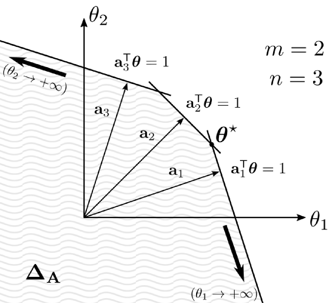
(a)

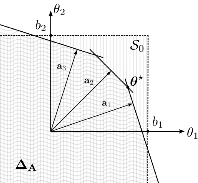
(b)

Figure 1: Motivation for the choice of ${\mathcal{S}_{0}}$ set in the $\beta_{1.5}$-divergence case with $\mathcal{I}_{0}=\emptyset$. a) The thick arrows show directions along which $\theta_{i}\to+\infty$ and, as a consequence, the singular values of the Hessian $\nabla^{2}D_{\lambda}(\bm{\mathrm{\theta}})$ tend to zero. b) Upper-bounding $\theta_{i}$ solves the problem.

The resulting local strong concavity bounds $\alpha_{\Delta_{\mathbf{A}}\cap{\mathcal{S}_{0}}}$ (Proposition 28) and $\alpha_{\mathcal{B}(\bm{\mathrm{\theta}},r)\cap{\mathcal{S}_{0}}}$ (Proposition 29) are presented in Table 1. The dual update discussed in Section 4.1 is also adapted in view of ${\mathcal{S}_{0}}$ (Proposition 30).

4.2.2 $\beta=1$ Kullback-Leibler Divergence Case

For the Kullback-Leibler divergence case, the $i$-th eigenvalue of the Hessian $\nabla^{2}D_{\lambda}(\bm{\mathrm{\theta}})$ is given by (see Section D.4) :

$$\sigma_{i}(\theta_{i})=-\lambda^{2}\frac{y_{i}}{(1+\lambda\theta_{i})^{2}}.$$ (40)

One can see that the eigenvalues are all non-positive, but may vanish in two cases: 1) when $|\theta_{i}|\rightarrow+\infty$. 2) when $y_{i}=0$. This means that, like before, the dual function is not globally strongly concave. The first problem is prevented when we restrict ourselves to any bounded set, which is the case for both $\mathcal{B}(\bm{\mathrm{\theta}},r)$ and $\Delta_{\mathbf{A}}$. We recall that in this particular case $\Delta_{\mathbf{A}}=\{\bm{\mathrm{\theta}}\in\mathbb{R}^{m}~{}|~{}\mathbf{A}^{\sf T}\bm{\mathrm{\theta}}\leq\bm{\mathrm{1}},~{}\bm{\mathrm{\theta}}\geq-\bm{\mathrm{1}}/\lambda\}$ is indeed bounded under the assumptions made on $\mathbf{A}$ (see equation (183) in Section D.4). However, the case $y_{i}=0$ remains a problem and, once again, the application of the proposed local approach requires the definition of some additional constraint set ${\mathcal{S}_{0}}$.

Fortunately, for coordinates $i\in\mathcal{I}_{0}$, the dual solution is trivially determined. Indeed, the primal-dual link in optimality condition (9) gives that $\theta_{i}^{\star}=-1/\lambda$ (see equation (168) in Section D.4). This leads us to the following constraint set (Proposition 34):

$${\mathcal{S}_{0}}=\{\bm{\mathrm{\theta}}\in\mathbb{R}^{m}~{}|~{}\bm{\mathrm{\theta}}_{\mathcal{I}_{0}}=-\bm{\mathrm{1}}/\lambda\}.$$ (41)

Note that ${\mathcal{S}_{0}}$ reduces to a singleton on coordinates $i\in\mathcal{I}_{0}$ and, from Proposition 11, the corresponding eigenvalues of $\nabla^{2}D_{\lambda}$ can be neglected. Moreover, $\bm{\mathrm{\theta}}^{\star}\in{\mathcal{S}_{0}}$, as required. This set ${\mathcal{S}_{0}}$ allows us to compute the local bounds $\alpha_{\Delta_{\mathbf{A}}\cap{\mathcal{S}_{0}}}$ (Proposition 35) and $\alpha_{\mathcal{B}(\bm{\mathrm{\theta}},r)\cap{\mathcal{S}_{0}}}$ (Proposition 36). Additionally, the dual update is adapted considering ${\mathcal{S}_{0}}$ in Proposition 37 and an improved screening test is defined in Proposition 38. All these quantities are reported in Table 1.

In a previous paper (Dantas et al., 2021), we addressed the KL particular case and proposed a local bound $\alpha_{\Delta_{\mathbf{A}}\cap{\mathcal{S}_{0}}}$ for a screening approach similar to Algorithm 2. However, the bound proposed here is far superior than the previous one, as this will be demonstrated in the experimental section. Moreover, the iterative refinement approach in Algorithm 3 was not a part of Dantas et al. (2021) and no bound $\alpha_{\mathcal{B}(\bm{\mathrm{\theta}},r)\cap{\mathcal{S}_{0}}}$ was provided.

4.2.3 Logistic Case

In this case, the $i$-th eigenvalue of the Hessian $\nabla^{2}D_{\lambda}(\bm{\mathrm{\theta}})$ is given by (see Section D.2):

$$\sigma_{i}\left(\theta_{i}\right)=-\frac{\lambda^{2}}{(y_{i}-\lambda\theta_{i})(1-y_{i}+\lambda\theta_{i})}.$$ (42)

Similarly to the quadratic case, the dual function is globally strongly concave as the eigenvalues never vanish. For this reason, we can simply take ${\mathcal{S}_{0}}=\mathbb{R}^{m}$. On the other hand, differently from the quadratic case, the eigenvalues are not constant and the proposed local approach may lead to better strong-concavity bounds.

Indeed, the local strong-concavity bound $\alpha_{\Delta_{\mathbf{A}}}$ (Proposition 22) does improve upon the global bound depending on the regularization parameter $\lambda$. More precisely, it improves upon the global constant $\alpha=4\lambda^{2}$ (see Table 1) for all

$$\lambda<\frac{1}{2\|\mathbf{A}^{\dagger}\|_{1}}.$$

where $\mathbf{A}^{\dagger}$ denotes the right pseudo-inverse of $\mathbf{A}$. It is important to mention that the proposed $\alpha_{\Delta_{\mathbf{A}}}$ uses the supplementary assumption that $\mathbf{A}$ is full rank with $\operatorname{rank}(\mathbf{A})=\min(n,m)$. If this hypothesis is not fullfiled, one can always initialize Algorithms 2 and 3 with the global bound $\alpha=4\lambda^{2}$. When deploying Algorithm 3, this bound will be automatically refined during the iterations thanks to the local bound $\alpha_{\mathcal{B}(\bm{\mathrm{\theta}},r)}$ (Proposition 23).

	$\beta=2$ (quadratic)	$\beta=1.5$	$\beta=1$ (Kullback-Leibler)	Logistic
$F(\mathbf{A}\bm{\mathrm{x}})$	$\frac{1}{2}\|\bm{\mathrm{y}}-\mathbf{A}\bm{\mathrm{x}}\|_{2}^{2}$	$\begin{array}[]{r}\frac{4}{3}\|\bm{\mathrm{y}}\|_{1.5}^{1.5}+\frac{2}{3}\|\mathbf{A}\bm{\mathrm{x}}+\epsilon\|_{1.5}^{1.5}\\ -2\bm{\mathrm{y}}^{\sf T}(\mathbf{A}\bm{\mathrm{x}}+\epsilon)^{0.5}\end{array}$	$\bm{\mathrm{y}}^{\sf T}\log(\frac{\bm{\mathrm{y}}}{\mathbf{A}\bm{\mathrm{x}}+\epsilon})+\bm{\mathrm{1}}^{\sf T}(\mathbf{A}\bm{\mathrm{x}}+\epsilon-\bm{\mathrm{y}})$	$\bm{\mathrm{1}}^{\sf T}\log\left(1+{\rm e}^{\mathbf{A}\bm{\mathrm{x}}}\right)-\bm{\mathrm{y}}^{\sf T}\mathbf{A}\bm{\mathrm{x}}$
$\mathcal{C}$	$\mathbb{R}^{n}$	$\mathbb{R}_{+}^{n}$	$\mathbb{R}_{+}^{n}$	$\mathbb{R}^{n}$
$D_{\lambda}(\bm{\mathrm{\theta}})$	$\frac{1}{2}\left(\|\bm{\mathrm{y}}\|_{2}^{2}-\|\bm{\mathrm{y}}-\lambda\bm{\mathrm{\theta}}\|_{2}^{2}\right)$	$\begin{array}[]{l}\frac{1}{6}\|\lambda\bm{\mathrm{\theta}}\|_{3}^{3}-\frac{1}{6}\|(\lambda\bm{\mathrm{\theta}})^{2}+4\bm{\mathrm{y}}\|_{1.5}^{1.5}\\ \qquad+\lambda\bm{\mathrm{\theta}}^{\sf T}\bm{\mathrm{y}}+\frac{4}{3}\|\bm{\mathrm{y}}\|_{1.5}^{1.5}-\epsilon\lambda\bm{\mathrm{\theta}}^{\sf T}\bm{\mathrm{1}}\end{array}$	$\bm{\mathrm{y}}^{\sf T}\log(1+\lambda\bm{\mathrm{\theta}})-\lambda\epsilon\bm{\mathrm{\theta}}^{\sf T}\bm{\mathrm{1}}$	$\begin{array}[]{l}(\bm{\mathrm{y}}\!-\!\lambda\bm{\mathrm{\theta}}\!-\!1)^{\sf T}\log(1\!-\!\bm{\mathrm{y}}\!+\!\lambda\bm{\mathrm{\theta}})\\ \qquad-(\bm{\mathrm{y}}\!-\!\lambda\bm{\mathrm{\theta}})^{\sf T}\log(\bm{\mathrm{y}}\!-\!\lambda\bm{\mathrm{\theta}})\end{array}$
$\operatorname{dom}(D_{\lambda})$	$\mathbb{R}^{m}$	$\mathbb{R}^{m}$	$\{\bm{\mathrm{\theta}}\in\mathbb{R}^{m}~{}|~{}\bm{\mathrm{\theta}}\geq-\bm{\mathrm{1}}/\lambda\}$	$\{\bm{\mathrm{\theta}}\in\mathbb{R}^{m}~{}|~{}\bm{\mathrm{y}}-1\leq\lambda\bm{\mathrm{\theta}}\leq\bm{\mathrm{y}}\}$
$\Delta_{\mathbf{A}}$	$\{\bm{\mathrm{\theta}}\!\in\!\mathbb{R}^{m}|~{}\|\mathbf{A}^{\sf T}\bm{\mathrm{\theta}}\|_{\infty}\!\leq\!1\}$	$\{\bm{\mathrm{\theta}}\in\mathbb{R}^{m}~{}|~{}\mathbf{A}^{\sf T}\bm{\mathrm{\theta}}\leq\bm{\mathrm{1}}\}$	$\{\bm{\mathrm{\theta}}\in\mathbb{R}^{m}~{}|~{}\mathbf{A}^{\sf T}\bm{\mathrm{\theta}}\leq\bm{\mathrm{1}},\bm{\mathrm{\theta}}\geq-\bm{\mathrm{1}}/\lambda\}$	$\begin{array}[]{l}\{\bm{\mathrm{\theta}}\in\mathbb{R}^{m}~{}|~{}\|\mathbf{A}^{\sf T}\bm{\mathrm{\theta}}\|_{\infty}\leq 1,\\ \qquad\qquad\;\;\bm{\mathrm{y}}-1\leq\lambda\bm{\mathrm{\theta}}\leq\bm{\mathrm{y}}\}\end{array}$
${\mathcal{S}_{0}}$	$\mathbb{R}^{m}$	$\begin{array}[]{ll}&\{\bm{\mathrm{\theta}}\in\mathbb{R}^{m}~{}|~{}\lambda\bm{\mathrm{\theta}}\leq\min(\bm{\mathrm{b}},\frac{\bm{\mathrm{y}}-\epsilon}{\sqrt{\epsilon}})\}\\ &b_{i}=\lambda\min_{j}\left(\frac{1-c\|\bm{\mathrm{a}}_{j}\|_{1}}{a_{ij}}\right)+\lambda c\\ &c=-\frac{1}{\lambda}\sqrt[3]{\frac{4\|\bm{\mathrm{y}}\|_{1.5}^{1.5}+2(m-1)\epsilon^{1.5}+3\epsilon}{1-3\epsilon}}\end{array}$	$\begin{array}[]{ll}\{\bm{\mathrm{\theta}}\in\mathbb{R}^{m}~{}|~{}\bm{\mathrm{\theta}}_{\mathcal{I}_{0}}=-\bm{\mathrm{1}}/\lambda\}\\ \text{with }\mathcal{I}_{0}=\{i\in[m]~{}|~{}y_{i}\!=\!0\}\end{array}$	$\mathbb{R}^{m}$
Primal-dual link	$\lambda\bm{\mathrm{\theta}}^{\star}=\bm{\mathrm{y}}-\mathbf{A}\bm{\mathrm{x}}^{\star}$	$\lambda\bm{\mathrm{\theta}}^{\star}=\frac{\bm{\mathrm{y}}}{\sqrt{\mathbf{A}\bm{\mathrm{x}}^{\star}+\epsilon}}-\sqrt{\mathbf{A}\bm{\mathrm{x}}^{\star}+\epsilon}$	$\lambda\bm{\mathrm{\theta}}^{\star}=\frac{\bm{\mathrm{y}}}{\mathbf{A}\bm{\mathrm{x}}^{\star}+\epsilon}-\bm{\mathrm{1}}$	$\lambda\bm{\mathrm{\theta}}^{\star}=\bm{\mathrm{y}}-\frac{{\rm e}^{\mathbf{A}\bm{\mathrm{x}}^{\star}}}{1+{\rm e}^{\mathbf{A}\bm{\mathrm{x}}^{\star}}}$
$\lambda_{\max}$	$\|\mathbf{A}^{\sf T}\bm{\mathrm{y}}\|_{\infty}$	$\max\left(\mathbf{A}^{\sf T}(\bm{\mathrm{y}}-\epsilon)\right)/\sqrt{\epsilon}$	$\max\left(\mathbf{A}^{\sf T}(\bm{\mathrm{y}}-\epsilon)\right)/\epsilon$	$\|\mathbf{A}^{\sf T}(\bm{\mathrm{y}}-\frac{1}{2})\|_{\infty}$
10cmDual update
$\bm{\mathrm{\Theta}}(\bm{\mathrm{x}})\!\in\!\Delta_{\mathbf{A}}\!\cap{\mathcal{S}_{0}}$	$\bm{\mathrm{\Xi}}\left((\bm{\mathrm{y}}-\mathbf{A}\bm{\mathrm{x}})/\lambda\right)$	$\min\left(\left[\bm{\mathrm{\Xi}}\left(\frac{\bm{\mathrm{y}}-\mathbf{A}\bm{\mathrm{x}}-\epsilon}{\lambda\sqrt{\mathbf{A}\bm{\mathrm{x}}+\epsilon}}\right)\right]_{i},~{}\frac{b_{i}}{\lambda},~{}\frac{y_{i}-\epsilon}{\lambda\sqrt{\epsilon}}\right)$	$\left\{\begin{array}[]{ll}\left[\bm{\mathrm{\Xi}}\left(\frac{1}{\lambda}\left(\frac{\bm{\mathrm{y}}}{\mathbf{A}\bm{\mathrm{x}}+\epsilon}-\bm{\mathrm{1}}\right)\right)\right]_{i}&\text{if }i\in\mathcal{I}_{0}^{\complement}\\ -\frac{1}{\lambda}&\text{if }i\in\mathcal{I}_{0}\end{array}\right.$	$\bm{\mathrm{\Xi}}\left(\frac{1}{\lambda}\left(\bm{\mathrm{y}}-\frac{{\rm e}^{\mathbf{A}\bm{\mathrm{x}}}}{1+{\rm e}^{\mathbf{A}\bm{\mathrm{x}}}}\right)\right)$
$\nabla^{2}D_{\lambda}(\bm{\mathrm{\theta}})$	$-\lambda^{2}\mathrm{Diag}\left(1,\dots,1\right)$	$-\lambda^{2}\mathrm{Diag}\left(\left[\frac{(\lambda\theta_{i})^{2}+2y_{i}}{\sqrt{(\lambda\theta_{i})^{2}+4y_{i}}}-\lambda\theta_{i}\right]_{i}\right)$	$-\lambda^{2}\mathrm{Diag}\left(\left[\frac{y_{i}}{(1+\lambda\theta_{i})^{2}}\right]_{i}\right)$	$-\lambda^{2}\mathrm{Diag}\left(\left[\frac{4}{1-4(\lambda\theta_{i}-y_{i}+\frac{1}{2})^{2}}\right]_{i}\right)$
$\alpha$ (global)	$\lambda^{2}$	–	–	$4\lambda^{2}$
$\alpha_{\Delta_{\mathbf{A}}\cap{\mathcal{S}_{0}}}$	$\lambda^{2}$	$\begin{array}[]{l}\min_{i\in[m]}-\sigma_{i}\left(\frac{1}{\lambda}\min\left(b_{i},\frac{y_{i}-\epsilon}{\sqrt{\epsilon}}\right)\right)\\ \sigma_{i}(\frac{z_{i}}{\lambda})=-\lambda^{2}\left(\frac{z_{i}^{2}+2y_{i}}{\sqrt{z_{i}^{2}+4y_{i}}}-z_{i}\right)\end{array}$	$\lambda^{2}\min_{i\in\mathcal{I}_{0}^{\complement}}\frac{y_{i}}{\left(\min_{j}\left(\frac{\lambda+\|\bm{\mathrm{a}}_{j}\|_{1}}{a_{ij}}\right)\right)^{2}}$	$\frac{4\lambda^{2}}{1-4\left(\min(\lambda\|\mathbf{A}^{\dagger}\|_{1},\frac{1}{2})-\frac{1}{2}\right)^{2}}$
$\alpha_{\mathcal{B}(\bm{\mathrm{\theta}},r)\cap{\mathcal{S}_{0}}}$	$\lambda^{2}$	$\begin{array}[]{l}\min_{i\in[m]}-\sigma_{i}(d_{i}/\lambda)\\ d_{i}=\min\left(\lambda(\theta_{i}+r),\;b_{i},\;\frac{y_{i}-\epsilon}{\sqrt{\epsilon}}\right)\end{array}$	$\lambda^{2}\min_{i\in\mathcal{I}_{0}^{\complement}}\frac{y_{i}}{(1+\lambda(\theta_{i}+r))^{2}}$	$\frac{4\lambda^{2}}{1-4([\min_{i}(|\lambda\theta_{i}-y_{i}+\frac{1}{2}|)-\lambda r]^{+})^{2}}$
10cmScreening test
($\Omega(\bm{\mathrm{x}})=\|\bm{\mathrm{x}}\|_{1}$)	$|\bm{\mathrm{a}}_{j}^{\sf T}\bm{\mathrm{\theta}}|+r\|\bm{\mathrm{a}}_{j}\|_{2}<1$	$\bm{\mathrm{a}}_{j}^{\sf T}\bm{\mathrm{\theta}}+r\|\bm{\mathrm{a}}_{j}\|_{2}<1$	$\bm{\mathrm{a}}_{j}^{\sf T}\bm{\mathrm{\theta}}+r\|[\bm{\mathrm{a}}_{j}]_{\mathcal{I}_{0}^{\complement}}\|_{2}<1$	$|\bm{\mathrm{a}}_{j}^{\sf T}\bm{\mathrm{\theta}}|+r\|\bm{\mathrm{a}}_{j}\|_{2}<1$

Table 1: Screening with three instances of $\beta$-divergence and logistic regression.

5 Experiments

In this section, our objective is to evaluate the proposed techniques in a diverse range of scenarios and provide essential insights for efficiently applying such techniques to other problems and settings. To that end, a wide range of experiments have been performed but only a representative subset of the results are presented in this section for the sake of conciseness and readability. The complete Matlab code is made available by the authors for the sake of reproducibility. Different simulation scenarios (not reported here) are also available for the interested reader.

Solvers.

For each of the three problems described in Section 4, namely logistic regression, KL divergence, and $\beta_{1.5}$-divergence, we deploy some popular solvers from the literature in their standard form (i.e., without screening) as well as within the three mentioned screening approaches: the existing dynamic Gap Safe approach in Algorithm 1 (when applicable) and the proposed screening methods with local strong concavity bounds in Algorithms 2 and 3. Screening is performed at every iteration after the solver update. Three different categories of solvers are used: coordinate descent (CoD) (Friedman et al., 2010; Hsieh and Dhillon, 2011; Yuan et al., 2010), multiplicative update (MU) yielding from majorization-minimization (Févotte and Idier, 2011) and proximal gradient algorithms (Harmany et al., 2012). The chosen solvers and the corresponding variations for each particular case are listed in Table 2.

Data Sets.

Well-suited data sets have been chosen according to each considered problem (see Table 2). The Leukemia binary classification data set (Golub et al., 1999) is used for the logistic regression case. For the KL case, the NIPS papers word count data set (Globerson et al., 2007) is considered. For the $\beta$-divergence case, we use the Urban hyperspectral image data set (Jia and Qian, 2007), since the $\beta$-divergence (especially with $\beta=1.5$) was reported to be well-suited for this particular type of data (Févotte and Dobigeon, 2015). Additional details are given in the following respective sections.

Problem	Solvers	Variations	Data
Logistic	CoD	[c][1cm][c]10cmNo screening, Alg. 1 (DGS),
Alg. 2 (G-DGS), Alg. 3 (R-DGS)	10cmBinary classification
(Leukemia data set)
KL	10cmMU, CoD,
Prox. Grad.	[c][1cm][c]10cmNo screening,
Alg. 2 (G-DGS), Alg. 3 (R-DGS)	10cmCount data
(NIPS papers data set)
$\beta=1.5$	MU	[c][1cm][c]10cmNo screening,
Alg. 2 (G-DGS), Alg. 3 (R-DGS)	10cmHyperspectral data
(Urban image)

Table 2: Experimental scenarios

Evaluation.

To compare the tested approaches, two main performance measures are used

1. Screening rate: how many (and how quickly) inactive coordinates are identified and eliminated by the compared screening strategies.

2. Execution time: the impact of screening in accelerating the solver’s convergence.

Table 3 specifies the explored values of two parameters with decisive impact in the performance measures. We set the “smoothing” parameter of $\beta_{1.5}$ and KL divergence to $\epsilon=10^{-6}$. Remaining problem parameters are fixed by the choice of the data set: problem dimensions ($m,n$) and data distribution (both the input vector $\bm{\mathrm{y}}$ and matrix $\mathbf{A}$).

Parameter	Range
Regularization ($\lambda/\lambda_{\max}$)	$[10^{-3},1]$
Stopping criterion ($\varepsilon_{\operatorname{gap}}$)	$\{10^{-7},10^{-5}\}$

Table 3: Simulation parameters and explored values.

This section is organized as follows: the particular cases of logistic regression, $\beta_{1.5}$-divergence and Kullback-Leibler divergence are treated respectively in Sections 5.1, 5.2 and 5.3. Other worth-mentioning properties of the proposed approaches are discussed in Section 5.4, notably the robustness of Algorithm 3 to the initialization of the strong concavity bound.

5.1 Logistic Regression

This example is particularly interesting as it allows to compare all screening approaches (Algorithms 1, 2 and 3). The classic Leukemia binary classification data set is used in the experiments, leading to a matrix $\mathbf{A}$ with dimensions $(m\times n)=(71\times 7129)$, whose columns are re-normalized to unit-norm. Vector $\bm{\mathrm{y}}$ contains the binary labels $\{0,1\}$ of each sample. A coordinate descent algorithm (Tseng and Yun, 2009) is used to optimize problem (24)—same as used by Ndiaye et al. (2017).

Figures 2(a) and 2(b) show the screening ratio (number of screened coordinates divided by the total number of coordinates) as a function of the iteration number, Figures 2(c) and 2(d) show the convergence rate (duality gap) as a function of the execution time and Figure 3 depicts relative execution times (where the solver without screening is taken as the reference) as a function of the regularization parameter. Figures 2(a) and 2(b) show a clear hierarchy between Algorithms 1, LABEL:, 2 and 3 in terms of screening performance, from worst to best. The difference is particularly pronounced at lower regularizations—cf. plot with $\lambda/\lambda_{\max}=10^{-3}$. As regularization grows, Algorithms 1 and 2 become equivalent ($\lambda/\lambda_{\max}=10^{-2}$) and later, around $\lambda/\lambda_{\max}=10^{-1}$, all approaches become equivalent. The first mentioned transition point, where Algorithms 1 and 2 become equivalent, can be theoretically predicted at $\lambda=(2\|\mathbf{A}^{\dagger}\|_{1})^{-1}$, as discussed in Section 4.2.3. In the reported example this corresponds to $\lambda=1.2\!\times\!10^{-2}\lambda_{\max}$. This threshold is depicted as a vertical dotted line in Figure 3 and it accurately matches the experimental results.

The discussed screening performances translate quite directly in terms of execution times, as shown in Figures 2(c) and 2(d). Figure 3 shows the relative execution times, where the basic solver (without screening) is taken as the reference, for a range of regularisation values at given convergence threshold ($\varepsilon_{\operatorname{gap}}=\{10^{-5},10^{-7}\}$). A typical behavior of screening techniques is observed: the smaller the convergence tolerance, the more advantageous screening becomes. Indeed, a smaller convergence tolerance leads to a larger number of iterations in the final optimization stage, where most coordinates are already screened out. A considerable speedup is obtained with Algorithm 3 in comparison to the other approaches in a wide range of regularization values and, in worst-case scenario, it is equivalent to other screening approaches (i.e., no significant overhead is observed). These results indicate that the proposed Algorithm 3 (R-DGS) should be preferred over the other approaches in this particular problem.

Similar results were obtained with other binary classification data sets from LIBSVM like the colon-cancer data set and the Reuters Corpus Volume I (rcv1.binary) data set.

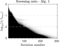
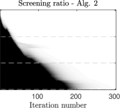
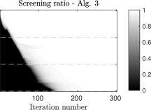
(a) Screening ratio against iterations for $\lambda/\lambda_{\max}\in[10^{-1},10^{-3}]$ (the lighter, the more screened coordinates), for Algorithms 1 to 3.

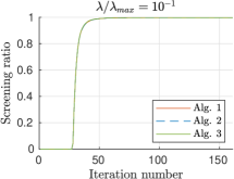
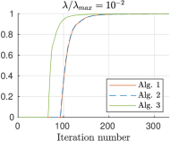
(b) Screening ratio against iterations for fixed regularization $\lambda/\lambda_{\max}=\{10^{-1},10^{-2},10^{-3}\}$, corresponding to the dotted slices in Figure 2(a).

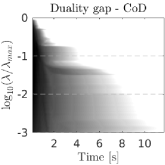
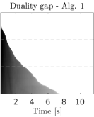
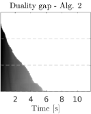
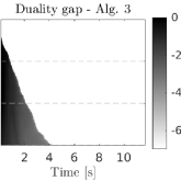
(c) Convergence rate (duality gap) against execution time for $\lambda/\lambda_{\max}\in[10^{-1},10^{-3}]$ (the lighter, the closer to convergence). Left to right: Coordinate Descent solver alone and in Algorithms 1 to 3.

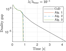
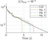
(d) Duality gap against time for fixed regularization $\lambda/\lambda_{\max}=\{10^{-1},10^{-2},10^{-3}\}$, corresponding to dotted slices in Figure 2(c).

Figure 2: Sparse logistic regression of Leukemia data set using Coordinate Descent and screening.

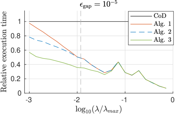
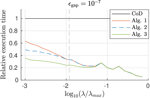
Figure 3: Sparse logistic regression on Leukemia data set using Coordinate Descent and screening. Relative execution times for $\lambda/\lambda_{\max}\in[10^{-3},1]$ (the smaller value, the faster) with convergence criterion $\varepsilon_{\operatorname{gap}}=10^{-5}$ (left) and $\varepsilon_{\operatorname{gap}}=10^{-7}$ (right).

5.2 $\beta_{1.5}$ Divergence

In this section, we use the Urban data set which is a ($307\times 307$)-pixel hyperspectral image with $162$ spectral bands per pixel. For the experiments, the input signal $\bm{\mathrm{y}}\in\mathbb{R}^{162}$ is given by a randomly-selected pixel from the image and the dictionary matrix $\mathbf{A}\in\mathbb{R}^{162\times 5000}$ is made of a uniformly-distributed random subset of $5000$ of the remaining pixels. Therefore, the goal is to reconstruct a given pixel (in $\bm{\mathrm{y}}$) as a sparse combination of other pixels from the same image, akin to archetypal analysis (Cutler and Breiman, 1994). The multiplicative MM algorithm described in (Févotte and Idier, 2011) is used to solve problem (22).

Figures 4(a) and 4(b) show the screening performance for Algorithms 2 and 3. Here, there is an even more pronounced difference between the two approaches (compared to the logistic regression case in Section 5.1) for the entire range of regularization values. Note that Algorithm 2 does not screen at all for $\lambda/\lambda_{\max}\leq 10^{-2}$, as opposed to Algorithm 3. This means that the refinement strategy in the latter approach manages to significantly improve, along the iterations, the initial strong-concavity bound (kept constant by the former). Even in highly-regularized scenarios, the screening ratio grows significantly faster with Algorithm 3.

A similar behavior is observed in Figures 4(c) and 4(d) regarding execution times. Because no screening is performed by Algorithm 2 at regularization $\lambda/\lambda_{\max}=10^{-2}$ (and below), no speedup is obtained w.r.t. the basic solver—there is even a slight overhead due to unfruitful screening tests calculations. Algorithm 2 only provides speedup over the basic solver for more regularized scenarios. Algorithm 3, in turn, provides acceleration over the entire regularization range and significantly outperforms both the basic solver and Algorithm 2. The previous observations are summarized in Figure 4(e) for normalized execution times.

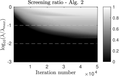
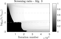
(a) Screening ratio against iterations for $\lambda/\lambda_{\max}\in[10^{-1},10^{-3}]$ (the lighter, the more screened coordinates) for Algorithms 2 and 3.

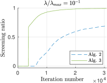
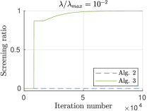
(b) Screening ratio against iterations for fixed regularization $\lambda/\lambda_{\max}=10^{-1}$ (left) and $\lambda/\lambda_{\max}=10^{-2}$ (right), corresponding to the dotted slices in Figure 4(a).

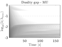
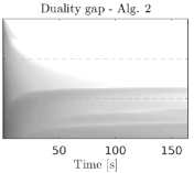
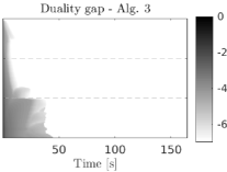
(c) Convergence rate (duality gap) against execution time for $\lambda/\lambda_{\max}\in[10^{-1},10^{-3}]$ (the lighter, the closer to convergence). From left to right: MU solver alone and Algorithms 2 and 3.

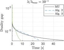
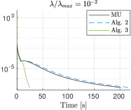
(d) Duality gap against time for regularization $\lambda/\lambda_{\max}=10^{-1}$ (left) and $\lambda/\lambda_{\max}=10^{-2}$ (right), corresponding to the dotted slices in Figure 4(c).

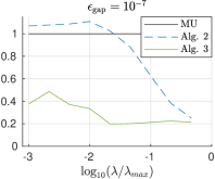
(e) Relative execution times for $\lambda/\lambda_{\max}\in[10^{-3},1]$.

Figure 4: Sparse non-negative hyperspectral decomposition using the Urban data set with $\beta=1.5$ and MU.

5.3 Kullback-Leibler Divergence

We here consider the NIPS papers word counts data set (Globerson et al., 2007). The input vector $\bm{\mathrm{y}}$ is a randomly selected column of the data matrix. The remaining data forms matrix $\mathbf{A}$ (of size $2483\times 14035$), after removing any all-zero rows and renormalizing all columns to unit-norm. Three standard optimization algorithms of distinct types have been used to solve problem (23): the multiplicative MM algorithm of Lee and Seung (2001); Févotte and Idier (2011), the coordinate descent of Hsieh and Dhillon (2011) and the proximal gradient descent of Harmany et al. (SPIRAL, 2012). As the different solvers lead to qualitatively similar results, we have chosen to only report the results for the SPIRAL method in order to avoid redundancy. Yet, for completeness, speedup results for all solvers are summarized in Table 4.

Differently from the previous cases, there is no difference between Algorithms 2 and 3 here. This indicates that: 1) the strong concavity constant does not vary significantly within the dual feasible set while approaching the dual solution and 2) the initial bound for $\alpha_{\Delta_{\mathbf{A}}\cap{\mathcal{S}_{0}}}$ given in Proposition 35 is nearly tight. This fact is verified both in terms of screening performance in Figures 5(a) and 5(b) and convergence time in Figures 5(c) and 5(d).

Nonetheless, we still observe significant speedups w.r.t. the basic solver, which proves the interest of the proposed techniques (see Figures 5(c) and 5(d) and Table 4). Acceleration by a factor of 20 are reported in Table 4 with remarkably stable results across the different regularization regimes. The obtained results are also about 3 times better than those reported in our previous work (Dantas et al., 2021), which corresponds to Algorithm 2 with a different bound for $\alpha_{\Delta_{\mathbf{A}}\cap{\mathcal{S}_{0}}}$. This indicates that the new strong concavity bound derived in the present paper is significantly tighter than the one given in (Dantas et al., 2021). Indeed, a difference of around two orders of magnitude was observed experimentally between the two bounds.

(a) Screening ratio against iterations for $\lambda/\lambda_{\max}\in[10^{-1},10^{-3}]$ (the lighter, the more screened coordinates), for Algorithms 2 and 3.

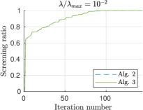
(b) Screening ratio against iterations for fixed regularization $\lambda/\lambda_{\max}=10^{-1}$ (left) and $\lambda/\lambda_{\max}=10^{-2}$ (right), corresponding to the dotted slices in Figure 5(a).

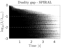
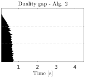
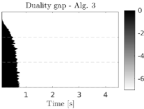
(c) Convergence rate (duality gap) against execution time for $\lambda/\lambda_{\max}\in[10^{-1},10^{-3}]$ (the lighter, the closer to convergence). From left to right: SPIRAL solver alone and in Algorithms 2 and 3.

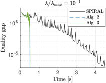
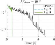
(d) Duality gap against time for regularization $\lambda/\lambda_{\max}=10^{-1}$ (left) and $\lambda/\lambda_{\max}=10^{-2}$ (right) corresponding to the dotted slices in Figure 5(c).

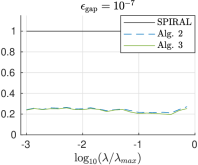
(e) Relative execution times for $\lambda/\lambda_{\max}\in[10^{-3},1]$.

Figure 5: Sparse KL regression using NIPS papers word count data set and the SPIRAL solver.

	$\lambda/\lambda_{\max}$	$10^{-1}$		$10^{-2}$		$10^{-3}$
	$\varepsilon_{\operatorname{gap}}$	$10^{-5}$	$10^{-7}$	$10^{-5}$	$10^{-7}$	$10^{-5}$	$10^{-7}$
	(Dantas et al., 2021)	2.77	3.21	2.50	2.83	2.26	2.53
SPIRAL	Algorithm 2	8.81	9.61	8.68	9.69	8.54	9.36
	Algorithm 3	8.75	9.55	8.61	9.61	8.44	9.24
	(Dantas et al., 2021)	4.19	5.35	4.06	5.13	4.12	5.06
CoD	Algorithm 2	17.03	19.70	16.45	18.73	15.95	18.26
	Algorithm 3	17.68	20.57	16.38	18.66	16.18	18.51
	(Dantas et al., 2021)	6.71	8.88	6.67	9.52	5.74	7.31
MU	Algorithm 2	17.24	23.56	20.46	26.58	18.28	23.73
	Algorithm 3	16.56	24.76	19.17	24.89	17.40	22.42

Table 4: Sparse KL regression: Average speedups (ratio of execution times without and with screening) using the NIPS papers data set. Dantas et al. (2021) is equivalent to Alg. 2 but with a worse $\alpha_{\Delta_{\mathbf{A}}\cap{\mathcal{S}_{0}}}$ constant.

5.4 A Deeper Look

5.4.1 Strong concavity bound evolution and robustness to initialization

Figure 6 shows the value of the strong concavity bound $\alpha$ over the iterations in the logistic regression scenario. While it is kept constant in Algorithms 1 and 2, it is progressively refined in Algorithm 3. To evaluate the robustness of the proposed refinement approach, we run Algorithm 3 with two different initializations: the global constant $\alpha_{\mathbb{R}^{m}}$ and the local constant $\alpha_{\Delta_{\mathbf{A}}\cap{\mathcal{S}_{0}}}$ (used respectively in Algorithms 1 and 2).

The left plot in Figure 6 shows that even with a poor initialization of $\alpha$, the proposed refinement approach will quickly improve the provided bound to match the better initialization, even though there is about one order of magnitude difference between both initializations. This indicates that the proposed refinement approach makes Algorithm 3 quite robust to the initialization of $\alpha$ and that the global $\alpha_{\mathbb{R}^{m}}$ constant can be used as an initialization of Algorithm 3 instead of the proposed $\alpha_{\Delta_{\mathbf{A}}\cap{\mathcal{S}_{0}}}$. This can be useful, for instance, when the additional full-rank assumption required by the latter bound is not met. More broadly, it suggests that Algorithm 3 can be applied to a new problem at hand without requiring an accurate initial estimation of the problem’s strong-concavity constant (provided, obviously, that one is capable of performing the refinement step, i.e., computing the bounds over $\mathcal{B}(\bm{\mathrm{\theta}},r)\cap{\mathcal{S}_{0}}$, which tends to be easier).

In the example depicted in Figure 6 the poor initialization of $\alpha$ is compensated dozens of iterations before screening even starts to take place and, as a consequence, no performance loss is inflicted by the poor initialization. Obviously, in other cases, this compensation might not be as quick, causing some harm to the final execution time. Yet, in any case, the proposed refinement approach significantly mitigates the impact of a poor initialization on the overall screening performance (and execution time).

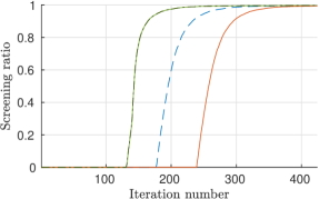
Figure 6: Left: evolution of the strong concavity bound $\alpha$ against iterations for the logistic regression problem, $\lambda/\lambda_{\max}=10^{-3}$. Algorithm 3 is initialized with local $\alpha_{\Delta_{\mathbf{A}}\cap{\mathcal{S}_{0}}}$ (solid light green line) and global $\alpha_{\mathbb{R}^{m}}$ (dash-dotted dark green line) bounds. Right: impact of the initialization over the screening performance.

5.4.2 Support identification for MU solver

Finally, we discuss and illustrate the power of screening for MU solvers using a small-size synthetic experiment (for readability). Multiplicative updates are very standard in (sparse) NMF, in particular with the general $\beta$-divergence (Févotte and Idier, 2011) but suffer from a well-known limitation. Because each coordinate (either of the dictionary or activation matrix) is multiplied by a strictly positive factor, convergence to zero values can only be asymptotical. This is shown in the left plot of Figure 7 which shows the value of each coordinate $x_{j}$ of the primal estimate $\bm{\mathrm{x}}$ over the iterations for the MU solver on the $\beta_{1.5}$-divergence case with dimensions $m=10$ and $n=20$. In practice, some arbitrary thresholding may be performed to force some entries to zero. However, such an ad-hoc operation may mistakenly cancel coordinates that belong to the support but happen to have small values. Conversely, the value of some coordinates might decrease very slowly with the iterations (see for instance the yellow line in Figure 7(a)) and may be mistakenly kept by such an arbitrary thresholding procedure. The proposed screening approach (Figure 7(b)) tackles this issue by introducing actual zeros to the solution with theoretical guarantees. Application of such strategies in NMF settings is an exciting and potentially fruitful perspective of this work.

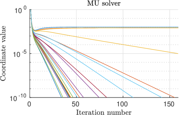
(a)

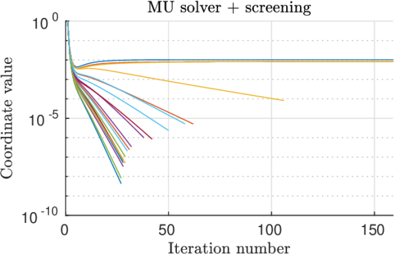
(b)

Figure 7: Coordinate values over the iterations of an MU solver, $\lambda/\lambda_{\max}=10^{-2}$ (a) without screening and (b) with screening. Each colored line corresponds to one coordinate, the line stops when the coordinate is screened.

6 Conclusion

In this paper, we proposed a safe screening framework that improves upon the existing Gap Safe screening approach, while extending its application to a wider range of problems—in particular, problems whose associated dual problem is not globally strongly concave.

Two screening algorithms have been proposed in this new framework, exploiting local properties of the involved functions. First, we defined a direct extension of the conventional dynamic screening approach, by replacing the global strong concavity bound $\alpha_{\mathbb{R}^{m}}$ by a local one $\alpha_{\Delta_{\mathbf{A}\cap{\mathcal{S}_{0}}}}$ in Algorithm 2. Noting that a reinforcement loop arises between the current safe sphere and the strong concavity bound within the sphere itself, we proposed the iterative refinement approach in Algorithm 3. By construction, the latter approach can only improve the initial strong-concavity bound, which makes it strictly superior to the former (the computational overhead due to the extra refinement loop was empirically observed to be negligible). Both proposed approaches lead to considerable speedups on several existing solvers and for various simulation scenarios.

Algorithm 3 can be superior to Algorithm 2 for two main reasons: 1) The strong concavity constant varies significantly within the dual feasible set. Therefore, refining it on the Gap Safe sphere (which shrinks over the iterations) may lead to significant improvements. 2) The initial strong concavity bound is loose (for instance, because it cannot be computed exactly and no tighter estimation is available). This initial handicap will then be progressively compensated by the refinement procedure in Algorithm 3.

The proposed framework is quite generic and not restricted to the four treated cases. Its application to other problems demands the completion of the following few steps: 1) the possible definition of a subset ${\mathcal{S}_{0}}$ (only for most challenging objective functions whose dual is not strongly concave on the entire dual feasible set); 2) the computation of an initial strong concavity bound $\alpha$ such that $\alpha\leq\alpha_{\Delta_{\mathbf{A}}\cap{\mathcal{S}_{0}}}$ (as observed experimentally, this bound does not need to be very precise); 3) the ability to compute the strong concavity bound on a $\ell_{2}$-ball (which possibly intersects with ${\mathcal{S}_{0}}$) for the refinement step. Other data-fidelity functions that could benefit from this framework include, for instance, the Huber loss, the Hinge (and squared Hinge) loss, or the Log-Cosh loss.

Although we restricted ourselves to the dynamic screening setting, nothing prevents this idea to be applied to more advanced Gap Safe screening configurations such as sequential screening (Ndiaye et al., 2017), working sets (Massias et al., 2017), dual extrapolation techniques (Massias et al., 2020), or even the stable safe screening framework (Dantas and Gribonval, 2019) in which approximation errors are tolerated in the data matrix.

Acknowledgments

This work was supported by the European Research Council (ERC FACTORY-CoG-6681839).

A Dual Problem and Optimality Conditions

A.1 Preliminaries

In order to prove Theorem 1 and its ensuing particular cases, we will use the classical result of Borwein and Lewis (2000, Theorem 3.3.5) or Rockafellar (1970, Theorem 31.3) which relates generic primal and dual problems with the Fenchel conjugates of the composing functions.

Generic Primal.

Consider a generic primal problem of the form:

$$\bm{\mathrm{x}}^{\star}\in\operatorname*{argmin}_{\bm{\mathrm{x}}\in\mathbb{R}^{n}}\underbrace{F(\mathbf{A}\bm{\mathrm{x}})+\lambda G(\bm{\mathrm{x}})}_{:=P_{\lambda}(\bm{\mathrm{x}})}$$ (43)

with $F$ (resp $G$) a closed proper and convex function on $\mathbb{R}^{m}$ (resp. $\mathbb{R}^{n}$). We denote by $P_{\lambda}$ the primal cost function.

Generic Dual.

The associated Lagrangian dual problem can be shown to be given by Borwein and Lewis (2000, Theorem 3.3.5)

$$\bm{\mathrm{\theta}}^{\star}\in \operatorname*{argmax}_{\bm{\mathrm{\theta}}\in\mathbb{R}^{m}}\underbrace{-F^{*}(-\lambda\bm{\mathrm{\theta}})-\lambda G^{*}({A^{\sf T}\bm{\mathrm{\theta}}})}_{=:D_{\lambda}(\bm{\mathrm{\theta}})}$$ (44)

where $D_{\lambda}(\bm{\mathrm{\theta}})$ denotes the dual (cost) function.

The optimality conditions are given by the following result (Bauschke and Combettes, 2011, Theorem 19.1).

Theorem 13.

Let $F:\mathbb{R}^{m}\to(-\infty,+\infty]$ and $G:\mathbb{R}^{n}\to(-\infty,+\infty]$ be convex lower semi-continuous, and let the linear operator $\mathbf{A}\in\mathbb{R}^{m\times n}$ be such that $\operatorname{dom}(G)\cap\mathbf{A}\operatorname{dom}(F)\neq\emptyset$. Then the following assertions are equivalent:

1. $\bm{\mathrm{x}}^{\star}$ is a primal solution, $\bm{\mathrm{\theta}}^{\star}$ is a dual solution and $P_{\lambda}(\bm{\mathrm{x}}^{\star})=D_{\lambda}(\bm{\mathrm{\theta}}^{\star})$ (i.e. strong duality holds).

2. $\mathbf{A}^{\sf T}\bm{\mathrm{\theta}}^{\star}\in\partial G(\bm{\mathrm{x}}^{\star})$ and $-\lambda\bm{\mathrm{\theta}}^{\star}\in\partial F(\mathbf{A}\bm{\mathrm{x}}^{\star})$.

Other useful results are given below.

Proposition 14 (Separable sum property of the Fenchel conjugate).

(Hiriart-Urruty and Lemaréchal, 1993b, Ch. X, Proposition 1.3.1 (ix)) Let $F=\sum_{i=1}^{m}f_{i}$ be coordinate-wise separable, then

$$F^{*}(\bm{\mathrm{u}})=\sum_{i=1}^{m}f_{i}^{*}(u_{i})$$

Proposition 15.

Let $F=\sum_{i=1}^{m}f_{i}$ be differentiable, then its gradient $\nabla F:\mathbb{R}^{m}\to\mathbb{R}^{m}$ is given by the (scalar) derivatives of $f_{i}$ as follows

$$\nabla F(\bm{\mathrm{z}})=[f_{1}^{\prime}(z_{1}),\dots,f_{m}^{\prime}(z_{m})]^{\sf T}\in\mathbb{R}^{m}.$$

Proposition 16 (Dual norm of a group-decomposable norm).

(Ndiaye, 2018, Proposition 21) Let $\mathcal{G}$ be a partition of $[n]$ and $\Omega(\bm{\mathrm{u}})=\sum_{g\in\mathcal{G}}\Omega_{g}(\bm{\mathrm{u}}_{g})$ be a group-decomposable norm. Its dual norm is given by $\overline{\Omega}(\bm{\mathrm{u}})=\max_{g\in\mathcal{G}}\overline{\Omega}_{g}(\bm{\mathrm{u}}_{g})$ where $\overline{\Omega}_{g}$ is the dual norm of $\Omega_{g}$

Proof  The result follows from Proposition 14: $\Omega^{*}(\bm{\mathrm{u}})=\sum_{g\in\mathcal{G}}\Omega_{g}^{*}(\bm{\mathrm{u}}_{g})=\sum_{g\in\mathcal{G}}\mathds{1}_{\overline{\Omega}_{g}(\bm{\mathrm{u}}_{g})\leq 1}=\mathds{1}_{\{\bm{\mathrm{u}}~{}|~{}\forall g\in\mathcal{G},~{}\overline{\Omega}_{g}(\bm{\mathrm{u}}_{g})\leq 1\}}=\mathds{1}_{\max_{g\in\mathcal{G}}\left(\overline{\Omega}_{g}(\bm{\mathrm{u}}_{g})\right)\leq 1}$. Since $\Omega^{*}(\cdot)=\mathds{1}_{\overline{\Omega}(\cdot)\leq 1}$ we conclude that $\overline{\Omega}(\bm{\mathrm{u}})=\max_{g\in\mathcal{G}}\left(\overline{\Omega}_{g}(\bm{\mathrm{u}}_{g})\right)$, which finishes the proof.  

A.2 Proof of Theorem 1

Note that in formulation (43), there are no constraints on the primal variable $\bm{\mathrm{x}}$. To make Problem (1) fit to this setting, we reformulate it as an unconstrained problem by using the indicator function $\mathds{1}_{\mathcal{C}}(\bm{\mathrm{x}})$. This strategy was used in Wang et al. (2019) for the non-negative Lasso problem and is extended here to a broader class of problems.

$$\bm{\mathrm{x}}^{\star}\in\operatorname*{argmin}_{\bm{\mathrm{x}}\in\mathbb{R}^{n}}\sum_{i=1}^{m}f_{i}([\mathbf{A}\bm{\mathrm{x}}]_{i})+\lambda\left(\Omega(\bm{\mathrm{x}})+\mathds{1}_{\mathcal{C}}(\bm{\mathrm{x}})\right).$$ (45)

Comparing (45) to (43), we have the following direct correspondences:

• $F(\mathbf{A}\bm{\mathrm{x}})=\sum_{i=1}^{m}f_{i}([\mathbf{A}\bm{\mathrm{x}}]_{i})$

• $G(\bm{\mathrm{x}})=G_{1}(\bm{\mathrm{x}})+G_{2}(\bm{\mathrm{x}})=\Omega(\bm{\mathrm{x}})+\mathds{1}_{\mathcal{C}}(\bm{\mathrm{x}})$

In this section, we address both cases $\mathcal{C}=\mathbb{R}^{n}$ and $\mathcal{C}=\mathbb{R}^{n}_{+}$, but we emphasize that the former case was previously treated in the literature (see Ndiaye (2018) for instance).

A.2.1 Dual problem

The dual problem in (4) is a direct application of the generic result in (44). We just need to evaluate the Fenchel conjugates $F^{*}$ and $G^{*}$ in our particular case described above.

$F=\sum_{i=1}^{m}f_{i}$ being coordinate-wise separable, we can apply Proposition 14:

$$F(\bm{\mathrm{z}})=\sum_{i=1}^{m}f_{i}(z_{i})~{}\Rightarrow~{}F^{*}(\bm{\mathrm{u}})=\sum_{i=1}^{m}f_{i}^{*}(u_{i})$$ (46)

Furthermore, we know that the Fenchel conjugate of a norm $\Omega$ is the indicator on the unit-ball of its corresponding dual norm $\overline{\Omega}$ (see for instance Bauschke and Combettes, 2011, Example 13.32):

$$G_{1}(\bm{\mathrm{x}})=\Omega(\bm{\mathrm{x}})~{}~{}\Rightarrow~{}~{}G_{1}^{*}(\bm{\mathrm{u}})=\mathds{1}_{\overline{\Omega}(\bm{\mathrm{u}})\leq 1}.$$

To conclude the proof, we need to consider the indicator function corresponding to the constraint set $\mathcal{C}$. The case $\mathcal{C}=\mathbb{R}^{n}$ is trivial since $\mathds{1}_{\mathbb{R}^{n}}(\bm{\mathrm{x}})\equiv 0$ and the Fenchel conjugate $G^{*}=G_{1}^{*}$ is given above. For the non-negativity contraint, $\mathcal{C}=\mathbb{R}_{+}^{n}$, we have (Wang et al., 2019, Lemma 18 (i)):

$$G_{2}(\bm{\mathrm{x}})=\mathds{1}_{\mathbb{R}_{+}^{n}}(\bm{\mathrm{x}})~{}~{}\Rightarrow~{}~{}G_{2}^{*}(\bm{\mathrm{u}})=\mathds{1}_{\mathbb{R}_{-}^{n}}(\bm{\mathrm{u}}).$$ (47)

Now, to calculate the conjugate of the sum $\Omega(\bm{\mathrm{x}})+\mathds{1}_{\mathbb{R}_{+}^{n}}(\bm{\mathrm{x}})$, we use a property that relates the conjugate of a sum to the so-called infimal convolution, denoted $\boxdot$, of the individual conjugates (Bauschke and Combettes, 2011, Proposition 15.2).

$$G^{*}(\bm{\mathrm{u}})=(G_{1}+G_{2})^{*}(\bm{\mathrm{u}})=(G_{1}^{*}\boxdot G_{2}^{*})(\bm{\mathrm{u}})=\mathds{1}_{\overline{\Omega}(\bm{\mathrm{u}})\leq 1}\boxdot\mathds{1}_{\mathbb{R}_{-}^{n}}(\bm{\mathrm{u}}).$$ (48)

Then, we use the fact that the infimal convolution of two indicator functions is the indicator of the Minkowski sum of both sets (Bauschke and Combettes, 2011, Example 12.3):

$$G^{*}(\bm{\mathrm{u}})=\mathds{1}_{\overline{\Omega}(\bm{\mathrm{u}})\leq 1}\boxdot\mathds{1}_{\mathbb{R}_{-}^{n}}(\bm{\mathrm{u}})=\mathds{1}_{\{\bm{\mathrm{u}}=\bm{\mathrm{a}}+\bm{\mathrm{b}}~{}|~{}\overline{\Omega}(\bm{\mathrm{a}})\leq 1,~{}\bm{\mathrm{b}}\leq 0\}}=\mathds{1}_{\overline{\Omega}([\bm{\mathrm{u}}]^{+})\leq 1}.$$ (49)

Remark 17.

The last step applies only because both conjugates $G^{*}_{1}$ and $G^{*}_{2}$ are indicator functions. This is no longer the case when we assume, for instance, a bounded-variable constraint of the form $x_{j}\in[-a_{j},b_{j}],~{}j\in[n]$.

This leads to the following results:

• For $\mathcal{C}=\mathbb{R}^{n}$, we have $G^{*}(\bm{\mathrm{u}})=G^{*}_{1}(\bm{\mathrm{u}})=\mathds{1}_{\overline{\Omega}(\bm{\mathrm{u}})\leq 1}$.

• For $\mathcal{C}=\mathbb{R}_{+}^{n}$, we have $G^{*}(\bm{\mathrm{u}})=(G_{1}+G_{2})^{*}(\bm{\mathrm{u}})=\mathds{1}_{\overline{\Omega}([\bm{\mathrm{u}}]^{+})\leq 1}$.

These can be written in a compact form using the non-linearity function $\phi$ as defined in (8):

$$G^{*}(\bm{\mathrm{u}})=\mathds{1}_{\overline{\Omega}(\phi(\bm{\mathrm{u}}))\leq 1}$$ (50)

Applying Proposition 16 for the dual of a group-separable norm $\overline{\Omega}(\phi(\bm{\mathrm{u}}))\!=\!\max_{g\in\mathcal{G}}\!\left(\overline{\Omega}_{g}(\phi(\bm{\mathrm{u}}_{g}))\right)$:

$$G^{*}(\bm{\mathrm{u}})=\mathds{1}_{\max_{g\in\mathcal{G}}\left(\overline{\Omega}_{g}(\phi(\bm{\mathrm{u}}_{g}))\right)\leq 1}.$$ (51)

The resulting dual problem is thus obtained by replacing $F^{*}$ (46) and $G^{*}$ (51) in the generic dual problem (44), that is

$$D_{\lambda}(\bm{\mathrm{\theta}})=-F^{*}(-\lambda\bm{\mathrm{\theta}})-\mathds{1}_{\overline{\Omega}(\phi(\mathbf{A}^{\sf T}\bm{\mathrm{\theta}}))\leq 1}.$$ (52)

Although in (44) the dual solution is not guaranteed to be unique, our assumption that $F$ is differentiable implies that $D_{\lambda}$ is strictly concave (Bauschke and Combettes, 2011, Proposition 18.10) which, in turn, implies the uniqueness of the dual solution.

Remark 18.

The constraint set being coordinate separable, we can always treat each group separately by restricting ourselves to the set of $n_{g}$ coordinates on group $g$. For simplicity, we derive the remaining results for $\Omega$ on $\mathbb{R}^{n}$ (the extension for groups with $\Omega_{g}$ being straightforward).

A.2.2 Optimality conditions

Optimality conditions (9) and (14) are a direct application of Theorem 13. Applying our definitions of $F$ and $G$, and knowing that $\partial F(\bm{\mathrm{z}})\!=\!\{\nabla F(\bm{\mathrm{z}})\}$ (a singleton as, by assumption, $F$ is differentiable) we have:

$$-\lambda\bm{\mathrm{\theta}}^{\star} =\nabla F(\mathbf{A}\bm{\mathrm{x}}^{\star})\!=\!\left[f_{1}^{\prime}([\mathbf{A}\bm{\mathrm{x}}^{\star}]_{1}),\dots,f_{m}^{\prime}([\mathbf{A}\bm{\mathrm{x}}^{\star}]_{m})\right]^{\sf T}$$ (53)

$$\mathbf{A}^{\sf T}\bm{\mathrm{\theta}}^{\star} \in\partial G(\bm{\mathrm{x}}^{\star})=\partial\Omega(\bm{\mathrm{x}}^{\star})+\partial\mathds{1}_{\mathcal{C}}(\bm{\mathrm{x}}^{\star})$$ (54)

To obtain (14) explicitly, the sum of subdifferentials in equation (54) is further developed below.

A.2.3 Sum of subdifferentials: $\partial\Omega(\mathbf{x})+\partial\mathds{1}_{\mathcal{C}}(\mathbf{x})$

Let us further develop the second optimality condition (54). It requires computing the subdifferentials of both $\Omega$ and $\mathds{1}_{\mathcal{C}}$, which are discussed below:

Proposition 19 (Subdifferential of a Norm).

(Bach et al., 2012, Proposition 1.2) The subdifferential of a norm $\Omega:\mathbb{R}^{n}\rightarrow\mathbb{R}$ at $\bm{\mathrm{x}}$ is given by

$$\partial\Omega(\bm{\mathrm{x}})=\left\{\begin{array}[]{lr}\{\bm{\mathrm{z}}\in\mathbb{R}^{n}~{}|~{}\overline{\Omega}(\bm{\mathrm{z}})\leq 1\},&~{}\text{if }~{}\bm{\mathrm{x}}=\bm{\mathrm{0}}\\ \{\bm{\mathrm{z}}\in\mathbb{R}^{n}~{}|~{}\overline{\Omega}(\bm{\mathrm{z}})=1~{}\text{ and }~{}\bm{\mathrm{z}}^{\sf T}\bm{\mathrm{x}}=\Omega(\bm{\mathrm{x}})\},&~{}\text{otherwise.}\end{array}\right.$$ (57)

Proposition 20 (Subdifferential of an indicator function).

(Bauschke and Combettes, 2011, Example 16.13) The subdifferential at point $\bm{\mathrm{x}}$ of the indicator of a set $\mathcal{C}$ is given by the normal cone of $\mathcal{C}$ at $\bm{\mathrm{x}}$, denoted $N_{\mathcal{C}}(\bm{\mathrm{x}})$:

$$\partial\mathds{1}_{\mathcal{C}}(\bm{\mathrm{x}})=N_{\mathcal{C}}(\bm{\mathrm{x}})=\left\{\begin{array}[]{lr}\{\bm{\mathrm{z}}\in\mathbb{R}^{n}~{}|~{}\bm{\mathrm{z}}^{\sf T}\bm{\mathrm{x}}\geq\bm{\mathrm{z}}^{\sf T}\bm{\mathrm{w}},~{}\forall\bm{\mathrm{w}}\in\mathcal{C}\}&\text{if }\bm{\mathrm{x}}\in\mathcal{C}\\ \emptyset&\text{otherwise.}\end{array}\right.$$ (60)

In particular, $N_{\mathcal{C}}(\bm{\mathrm{x}})=\{\bm{\mathrm{0}}\},\forall\bm{\mathrm{x}}\in\operatorname*{int}(\mathcal{C})$.

When it comes to the constraint sets considered in this paper, we have:

$$\partial\mathds{1}_{\mathbb{R}^{n}}\equiv\{0\}.$$ (61)

$$\partial\mathds{1}_{R_{+}^{n}}(\bm{\mathrm{x}})=J_{1}\times\dots\times J_{n}, J_{j}=\left\{\begin{array}[]{ll}\emptyset&\text{if }x_{j}<0\\ (-\infty,0]&\text{if }x_{j}=0\\ \{0\}&\text{if }x_{j}>0.\end{array}\right.$$ with (65)

The case $\mathcal{C}=\mathbb{R}^{n}$ is trivial, since $\partial\mathds{1}_{\mathbb{R}^{n}}(\bm{\mathrm{x}})\equiv\{\bm{\mathrm{0}}\}$ and therefore $\partial\Omega(\bm{\mathrm{x}})+\partial\mathds{1}_{\mathbb{R}^{n}}(\bm{\mathrm{x}})=\partial\Omega(\bm{\mathrm{x}})$, which is given in equation (57). Let us now analyze the case $\mathcal{C}=\mathbb{R}_{+}^{n}$. First of all, note that the subdifferential $\partial\mathds{1}_{\mathbb{R}_{+}^{n}}(\bm{\mathrm{x}})$ in equation (65) can be rewritten in the following form:

$$\partial\mathds{1}_{R_{+}^{n}}(\bm{\mathrm{x}}) =\left\{\begin{array}[]{lll}\emptyset&\text{if }\bm{\mathrm{x}}\notin\mathbb{R}_{+}^{n}&\\ \{\bm{\mathrm{z}}\in\mathbb{R}^{n}~{}|~{}\bm{\mathrm{z}}\leq\bm{\mathrm{0}}\}=\mathbb{R}_{-}^{n}&\text{if }\bm{\mathrm{x}}=\bm{\mathrm{0}}&\\ \{\bm{\mathrm{z}}\in\mathbb{R}^{n}~{}|~{}\bm{\mathrm{z}}\leq\bm{\mathrm{0}}\text{ and }\bm{\mathrm{z}}^{\sf T}\bm{\mathrm{x}}=0\}&\text{otherwise}&\text{(i.e. }\bm{\mathrm{x}}\geq\bm{\mathrm{0}}\text{ and }\bm{\mathrm{x}}\neq\bm{\mathrm{0}}\text{).}\end{array}\right.$$ (69)

Therefore, the (Minkowski) sum of the subdifferential sets in equations (57) and (69) gives:

$$\partial\Omega(\bm{\mathrm{x}})+\partial\mathds{1}_{\mathbb{R}_{+}^{n}}(\bm{\mathrm{x}}) =\left\{\begin{array}[]{lll}\emptyset&~{}\text{if }~{}\bm{\mathrm{x}}\notin\mathbb{R}_{+}^{n}&\\ \{\bm{\mathrm{z}}=\bm{\mathrm{z}}_{1}+\bm{\mathrm{z}}_{2}~{}|~{}\overline{\Omega}(\bm{\mathrm{z}}_{1})\leq 1,~{}\bm{\mathrm{z}}_{2}\leq 0\},&~{}\text{if }~{}\bm{\mathrm{x}}=\bm{\mathrm{0}}&\\ \{\bm{\mathrm{z}}=\bm{\mathrm{z}}_{1}+\bm{\mathrm{z}}_{2}~{}|~{}\overline{\Omega}(\bm{\mathrm{z}}_{1})=1,~{}\bm{\mathrm{z}}_{1}^{\sf T}\bm{\mathrm{x}}=\Omega(\bm{\mathrm{x}}),\bm{\mathrm{z}}_{2}\leq 0,~{}\bm{\mathrm{z}}_{2}^{\sf T}\bm{\mathrm{x}}=0\},&~{}\text{otherwise}&\end{array}\right.$$ (73)

$$=\left\{\begin{array}[]{lll}\emptyset&~{}\text{if }~{}\bm{\mathrm{x}}\notin\mathbb{R}_{+}^{n}&\\ \{\bm{\mathrm{z}}\in\mathbb{R}^{n}~{}|~{}\overline{\Omega}([\bm{\mathrm{z}}]^{+})\leq 1\},&~{}\text{if }~{}\bm{\mathrm{x}}=\bm{\mathrm{0}}&\\ \{\bm{\mathrm{z}}\in\mathbb{R}^{n}~{}|~{}\overline{\Omega}([\bm{\mathrm{z}}]^{+})=1,~{}\bm{\mathrm{z}}^{\sf T}\bm{\mathrm{x}}=\Omega(\bm{\mathrm{x}})\},&~{}\text{otherwise}&\end{array}\right.$$ (77)

where, in the last equality, we have used the fact that $\bm{\mathrm{z}}_{1}^{\sf T}\bm{\mathrm{x}}=(\bm{\mathrm{z}}-\bm{\mathrm{z}}_{2})^{\sf T}\bm{\mathrm{x}}=\bm{\mathrm{z}}^{\sf T}\bm{\mathrm{x}}$, since $\bm{\mathrm{z}}_{2}^{\sf T}\bm{\mathrm{x}}=0$.

Comparing equations (57) and (77) respectively for $\mathcal{C}=\mathbb{R}^{n}$ and $\mathcal{C}=\mathbb{R}_{+}^{n}$, we can see that the sum $\partial\Omega+\partial\mathds{1}_{\mathcal{C}}$ for the considered constraint sets writes compactly as:

$$\partial\Omega(\bm{\mathrm{x}})+\partial\mathds{1}_{\mathcal{C}}(\bm{\mathrm{x}})=\left\{\begin{array}[]{lrl}\emptyset&~{}\text{if }~{}\bm{\mathrm{x}}\notin\mathcal{C}&\\ \{\bm{\mathrm{z}}\in\mathbb{R}^{n}~{}|~{}\overline{\Omega}(\phi(\bm{\mathrm{z}}))\leq 1\},&~{}\text{if }~{}\bm{\mathrm{x}}=\bm{\mathrm{0}}&\\ \{\bm{\mathrm{z}}\in\mathbb{R}^{n}~{}|~{}\overline{\Omega}(\phi(\bm{\mathrm{z}}))=1,~{}\bm{\mathrm{z}}^{\sf T}\bm{\mathrm{x}}=\Omega(\bm{\mathrm{x}})\},&~{}\text{otherwise}&\end{array}\right.$$ (81)

where $\phi$ is defined as in (8).

Applying the above results to equation (54), it takes the following form which corresponds to (14)

$$\left\{\begin{array}[]{lrl}\overline{\Omega}(\phi(\mathbf{A}^{\sf T}\bm{\mathrm{\theta}}^{\star}))\leq 1,&~{}\text{if }~{}\bm{\mathrm{x}}^{\star}=\bm{\mathrm{0}}&\\ \overline{\Omega}(\phi(\mathbf{A}^{\sf T}\bm{\mathrm{\theta}}^{\star}))=1,~{}~{}(\mathbf{A}^{\sf T}\bm{\mathrm{\theta}}^{\star})^{\sf T}\bm{\mathrm{x}}^{\star}=\Omega(\bm{\mathrm{x}}^{\star}),&~{}\text{otherwise}&\end{array}\right.$$ (84)

B Proof of Theorem 5

In this section we prove Theorem 5, i.e. given any feasible primal-dual pair $(\bm{\mathrm{x}},\bm{\mathrm{\theta}})\in{(\operatorname{dom}(P_{\lambda})\cap\mathcal{C})}\times(\Delta_{A}\cap\mathcal{S})$ and supposing $D_{\lambda}$ to be $\alpha_{\mathcal{S}}$-strongly concave on $\mathcal{S}$, we prove that a region

$$\mathcal{B}(\bm{\mathrm{\theta}},r),\quad\text{with }r=\sqrt{\frac{2\operatorname{Gap}_{\lambda}({\bm{\mathrm{x}}},{\bm{\mathrm{\theta}}})}{\alpha_{\mathcal{S}}}}$$ (85)

is safe, i.e. $\bm{\mathrm{\theta}}^{\star}\in\mathcal{B}(\bm{\mathrm{\theta}},r)$. Equivalently, we prove that $\|{\bm{\mathrm{\theta}}}-\bm{\mathrm{\theta}}^{\star}\|_{2}\leq r.$

The proof follows quite similarly to Ndiaye et al. (2017, Theorem 6). (except that we assume strong concavity of $D_{\lambda}$ exclusively on $\mathcal{S}$ instead of $\mathbb{R}^{m}$). From the $\alpha_{\mathcal{S}}$-strong concavity of $D_{\lambda}$ on $\mathcal{S}$ we have:

$$\forall(\bm{\mathrm{\theta}}^{\prime},\bm{\mathrm{\theta}}^{\prime\prime})\in\mathcal{S}\times\mathcal{S},\quad D_{\lambda}(\bm{\mathrm{\theta}}^{\prime\prime})\leq D_{\lambda}(\bm{\mathrm{\theta}}^{\prime})+\langle\nabla D_{\lambda}(\bm{\mathrm{\theta}}^{\prime}),\bm{\mathrm{\theta}}^{\prime\prime}-\bm{\mathrm{\theta}}^{\prime}\rangle-\frac{\alpha_{\mathcal{S}}}{2}\|\bm{\mathrm{\theta}}^{\prime\prime}-\bm{\mathrm{\theta}}^{\prime}\|_{2}^{2}.$$

In particular, we can take $\bm{\mathrm{\theta}}^{\prime}=\bm{\mathrm{\theta}}^{\star}$, $\bm{\mathrm{\theta}}^{\prime\prime}={\bm{\mathrm{\theta}}}$ (since we suppose ${\bm{\mathrm{\theta}}}\in\mathcal{S}$ and $\bm{\mathrm{\theta}}^{\star}\in\mathcal{S}$):

$$D_{\lambda}({\bm{\mathrm{\theta}}})\leq D_{\lambda}(\bm{\mathrm{\theta}}^{\star})+\langle\nabla D_{\lambda}(\bm{\mathrm{\theta}}^{\star}),{\bm{\mathrm{\theta}}}-\bm{\mathrm{\theta}}^{\star}\rangle-\frac{\alpha_{\mathcal{S}}}{2}\|\bm{\mathrm{\theta}}-{\bm{\mathrm{\theta}}}^{\star}\|_{2}^{2}.$$

By definition $\bm{\mathrm{\theta}}^{\star}$ maximizes $D_{\lambda}$ on $\Delta_{\mathbf{A}}$ and hence $\langle\nabla D_{\lambda}(\bm{\mathrm{\theta}}^{\star}),{\bm{\mathrm{\theta}}}-\bm{\mathrm{\theta}}^{\star}\rangle\leq 0$ (otherwise, ${\bm{\mathrm{\theta}}}-\bm{\mathrm{\theta}}^{\star}$ would be a feasible direction of improvement), which implies:

$$D_{\lambda}({\bm{\mathrm{\theta}}})\leq D_{\lambda}(\bm{\mathrm{\theta}}^{\star})-\frac{\alpha_{\mathcal{S}}}{2}\|\bm{\mathrm{\theta}}-{\bm{\mathrm{\theta}}}^{\star}\|_{2}^{2}.$$

By weak duality $D_{\lambda}(\bm{\mathrm{\theta}}^{\star})\leq P_{\lambda}(\bm{\mathrm{x}}^{\prime})$, $\forall\bm{\mathrm{x}}^{\prime}\in\operatorname{dom}(P_{\lambda})\cap\mathcal{C}$, and in particular for $\bm{\mathrm{x}}^{\prime}={\bm{\mathrm{x}}}$, giving:

$$D_{\lambda}({\bm{\mathrm{\theta}}}) \leq P_{\lambda}({\bm{\mathrm{x}}})-\frac{\alpha_{\mathcal{S}}}{2}\|\bm{\mathrm{\theta}}-\bm{\mathrm{\theta}}^{\star}\|_{2}^{2}$$

$$\underbrace{D_{\lambda}({\bm{\mathrm{\theta}}})-P_{\lambda}({\bm{\mathrm{x}}})}_{-G_{\lambda}({\bm{\mathrm{x}}},{\bm{\mathrm{\theta}}})} \leq-\frac{\alpha_{\mathcal{S}}}{2}\|\bm{\mathrm{\theta}}-{\bm{\mathrm{\theta}}}^{\star}\|_{2}^{2}$$

$$\frac{2}{\alpha_{\mathcal{S}}}G_{\lambda}({\bm{\mathrm{x}}},{\bm{\mathrm{\theta}}}) \geq\|\bm{\mathrm{\theta}}-{\bm{\mathrm{\theta}}}^{\star}\|_{2}^{2}$$

which holds for all ${\bm{\mathrm{x}}}\in\operatorname{dom}(P_{\lambda})\cap\mathcal{C},{\bm{\mathrm{\theta}}}\in\Delta_{\mathbf{A}}\cap\mathcal{S}$, concluding the proof.

C Proofs of Section 4.1

C.1 Proof of Proposition 9

Statement. 

$$\bm{\mathrm{0}}\in\operatorname*{argmin}_{\bm{\mathrm{x}}\in\mathcal{C}}P_{\lambda}(\bm{\mathrm{x}})\iff\lambda\geq\lambda_{\max}:=\overline{\Omega}\left(\phi\left(-\mathbf{A}^{\sf T}\nabla F(\bm{\mathrm{0}})\right)\right)$$ (86)

Proof  Writing our primal problem in an equivalent unconstrained form, we have

$$\operatorname*{argmin}_{\bm{\mathrm{x}}\in\mathbb{R}^{n}}F(\mathbf{A}\bm{\mathrm{x}})+\lambda\left(\Omega(\bm{\mathrm{x}})+\mathds{1}_{\mathcal{C}}(\bm{\mathrm{x}})\right):=P^{\operatorname{unc}}_{\lambda}(\bm{\mathrm{x}})$$

denoting $P^{\operatorname{unc}}_{\lambda}$ the unconstrained objective function, with $\operatorname*{argmin}_{\bm{\mathrm{x}}\in\mathbb{R}^{n}}P^{\operatorname{unc}}_{\lambda}(\bm{\mathrm{x}})\!=\!\operatorname*{argmin}_{\bm{\mathrm{x}}\in\mathcal{C}}P_{\lambda}(\bm{\mathrm{x}})$. From Fermat’s rule we have that

$$\bm{\mathrm{0}}\in\operatorname*{argmin}_{\bm{\mathrm{x}}\in\mathbb{R}^{n}}P^{\operatorname{unc}}_{\lambda}(\bm{\mathrm{x}}) \iff\bm{\mathrm{0}}\in\partial P^{\operatorname{unc}}_{\lambda}(\bm{\mathrm{0}})=\{\mathbf{A}^{\sf T}\nabla F(\bm{\mathrm{0}})\}+\lambda\left(\partial\Omega(\bm{\mathrm{0}})+\partial\mathds{1}_{\mathcal{C}}(\bm{\mathrm{0}})\right)$$

$$\iff-\mathbf{A}^{\sf T}\nabla F(\bm{\mathrm{0}})/\lambda\in\partial\Omega(\bm{\mathrm{0}})+\partial\mathds{1}_{\mathcal{C}}(\bm{\mathrm{0}}).$$

Using the expression of $\partial\Omega(\bm{\mathrm{x}})+\partial\mathds{1}_{\mathcal{C}}(\bm{\mathrm{x}})$ given in (81) we obtain

$$\bm{\mathrm{0}}\in\operatorname*{argmin}_{\bm{\mathrm{x}}\in\mathbb{R}^{n}}P^{\operatorname{unc}}_{\lambda}(\bm{\mathrm{x}})\iff\overline{\Omega}\left(\phi(-\mathbf{A}^{\sf T}\nabla F(\bm{\mathrm{0}}))\right)\leq\lambda,$$

which completes the proof.  

C.2 Proof of Lemma 10

Statement.  Assume that $\operatorname{dom}(D_{\lambda})$ is stable by contraction and let $\bm{\mathrm{\Xi}}:\mathbb{R}^{m}\rightarrow\mathbb{R}^{m}$ be the scaling operator defined by

$$\bm{\mathrm{\Xi}}(\bm{\mathrm{z}}):=\frac{\bm{\mathrm{z}}}{\max\left(\overline{\Omega}(\phi(\mathbf{A}^{\sf T}\bm{\mathrm{z}})),1\right)}.$$ (87)

Then, for any point $\bm{\mathrm{z}}\in\operatorname{dom}(D_{\lambda})$, we have $\bm{\mathrm{\Xi}}(\bm{\mathrm{z}})\in\Delta_{\mathbf{A}}$. Moreover, for any primal point $\bm{\mathrm{x}}\in\operatorname{dom}(P_{\lambda})$, we have that $\bm{\mathrm{z}}=(-\nabla F(\mathbf{A}\bm{\mathrm{x}})/\lambda)\in\operatorname{dom}(D_{\lambda})$ and therefore

$$\bm{\mathrm{\Xi}}(-\nabla F(\mathbf{A}\bm{\mathrm{x}})/\lambda)\in\Delta_{\mathbf{A}}.$$ (88)

Finally, if $F\in C^{1}$, then $\bm{\mathrm{\Xi}}(-\nabla F(\mathbf{A}\bm{\mathrm{x}})/\lambda)\rightarrow\bm{\mathrm{\theta}}^{\star}$ as $\bm{\mathrm{x}}\rightarrow\bm{\mathrm{x}}^{\star}$.

Proof  By definition of $\bm{\mathrm{\Xi}}$, one can see that $\bm{\mathrm{\Xi}}(\bm{\mathrm{z}})\leq\bm{\mathrm{z}}$ and, given the assumption that $\operatorname{dom}(D_{\lambda})$ is stable by contraction, we get that $\forall\bm{\mathrm{z}}\in\operatorname{dom}(D_{\lambda})$, $\bm{\mathrm{\Xi}}(\bm{\mathrm{z}})\in\operatorname{dom}(D_{\lambda})$. Combining this with the fact that $\overline{\Omega}\left(\phi(\mathbf{A}^{\sf T}\bm{\mathrm{\Xi}}(\bm{\mathrm{z}}))\right)\leq 1$ (by definition of $\bm{\mathrm{\Xi}}$), we obtain

$$\forall\bm{\mathrm{z}}\in\operatorname{dom}(D_{\lambda}),\;\bm{\mathrm{\Xi}}(\bm{\mathrm{z}})\in\Delta_{\mathbf{A}},$$ (89)

where we recall that $\Delta_{\mathbf{A}}=\{\bm{\mathrm{\theta}}\in\mathbb{R}^{m}~{}|~{}\overline{\Omega}(\phi(\mathbf{A}^{\sf T}\bm{\mathrm{\theta}}))\leq 1\}\cap\operatorname{dom}(D_{\lambda})$.

To complete the proof, it remains to show that, for any primal point $\bm{\mathrm{x}}\in\operatorname{dom}(P_{\lambda})$, $(-\nabla F(\mathbf{A}\bm{\mathrm{x}})/\lambda)\in\operatorname{dom}(D_{\lambda})$. Because $D_{\lambda}=-F^{*}(-\lambda\cdot)$, we get that $\bm{\mathrm{\theta}}\in\operatorname{dom}(D_{\lambda})\,\Longleftrightarrow\,-\lambda\bm{\mathrm{\theta}}\in\operatorname{dom}(F^{*})$. Now, let $\bm{\mathrm{x}}\in\operatorname{dom}(P_{\lambda})$, then

$$F^{*}(\nabla F(\mathbf{A}\bm{\mathrm{x}}))=\sup_{\bm{\mathrm{z}}\in\mathbb{R}^{m}}\left<\bm{\mathrm{z}},\nabla F(\mathbf{A}\bm{\mathrm{x}})\right>-F(\bm{\mathrm{z}})=\left<\mathbf{A}\bm{\mathrm{x}},\nabla F(\mathbf{A}\bm{\mathrm{x}})\right>-F(\mathbf{A}\bm{\mathrm{x}})<\infty.$$ (90)

(The sup is attained for vector(s) $\bm{\mathrm{z}}\in\mathbb{R}^{m}$ such that $\nabla F(\mathbf{A}\bm{\mathrm{x}})-\nabla F(\bm{\mathrm{z}})=0$, such as $\bm{\mathrm{z}}=\mathbf{A}\bm{\mathrm{x}}$.) This shows that $\nabla F(\mathbf{A}\bm{\mathrm{x}})\in\operatorname{dom}(F^{*})$ and thus that $(-\nabla F(\mathbf{A}\bm{\mathrm{x}})/\lambda)\in\operatorname{dom}(D_{\lambda})$.

Lastly, assuming that $F\in C^{1}$, we get by continuity of $\nabla F(\mathbf{A}\bm{\mathrm{x}})$ that $\nabla F(\mathbf{A}\bm{\mathrm{x}})\rightarrow\nabla F(\mathbf{A}\bm{\mathrm{x}}^{\star})$ as $\bm{\mathrm{x}}\rightarrow\bm{\mathrm{x}}^{\star}$ and, from the primal-dual link in optimality condition (9) we have that $-\nabla F(\mathbf{A}\bm{\mathrm{x}}^{\star})=\lambda\bm{\mathrm{\theta}}^{\star}$. Then, because $\bm{\mathrm{\theta}}^{\star}\in\Delta_{\mathbf{A}}$, the scaling factor in $\bm{\mathrm{\Xi}}$ is equal to 1 (by definition) which leads to $\bm{\mathrm{\Xi}}(-\nabla F(\mathbf{A}\bm{\mathrm{x}}^{\star})/\lambda)=-\nabla F(\mathbf{A}\bm{\mathrm{x}}^{\star})/\lambda=\bm{\mathrm{\theta}}^{\star}$. Finally, by continuity of $\bm{\mathrm{\Xi}}$ (which is a composition of continuous functions), we conclude that $\bm{\mathrm{\Xi}}(-\nabla F(\mathbf{A}\bm{\mathrm{x}})/\lambda)\rightarrow\bm{\mathrm{\theta}}^{\star}$ as $\bm{\mathrm{x}}\rightarrow\bm{\mathrm{x}}^{\star}$.  

C.3 Proof of Proposition 11

Statement.  Assume that $D_{\lambda}$ given in Theorem 1 is twice differentiable. Let $\mathcal{S}\in\mathbb{R}^{m}$ be a convex set and $\mathcal{I}=\{i\in[m]:\forall(\bm{\mathrm{\theta}},\bm{\mathrm{\theta}}^{\prime})\in\mathcal{S}^{2},\theta_{i}=\theta_{i}^{\prime}\}$ a (potentially empty) set of coordinates in which $\mathcal{S}$ reduces to a singleton. Then, $D_{\lambda}$ is $\alpha_{\mathcal{S}}$-strongly concave on $\mathcal{S}$ if and only if

$$0<\alpha_{\mathcal{S}}\leq\min_{i\in\mathcal{I}^{\complement}}\;-\sup_{\bm{\mathrm{\theta}}\in\mathcal{S}}\;\sigma_{i}(\theta_{i}),$$ (91)

where $\sigma_{i}(\theta_{i})=-\lambda^{2}(f_{i}^{*})^{\prime\prime}(-\lambda\theta_{i})$ is the (negative) i-th eigenvalue of the Hessian matrix $\nabla^{2}D_{\lambda}(\bm{\mathrm{\theta}})$.

Proof  First of all, let us recall that, from Theorem 1, $D_{\lambda}(\bm{\mathrm{\theta}})=-\sum_{i}f_{i}^{*}(-\lambda\theta_{i})$. Then by definition of strong concavity, $D_{\lambda}$ is $\alpha$-strongly concave on a set $\mathcal{S}\subset\mathbb{R}^{m}$ if and only if, $\forall(\bm{\mathrm{\theta}}^{\prime},\bm{\mathrm{\theta}})\in\mathcal{S}^{2}$,

$$\;D_{\lambda}(\bm{\mathrm{\theta}})\leq D_{\lambda}(\bm{\mathrm{\theta}}^{\prime})+\langle\nabla D_{\lambda}(\bm{\mathrm{\theta}}^{\prime}),\bm{\mathrm{\theta}}-\bm{\mathrm{\theta}}^{\prime}\rangle-\frac{\alpha^{2}}{2}\|\bm{\mathrm{\theta}}-\bm{\mathrm{\theta}}^{\prime}\|_{2}^{2}$$ (92)

$$\Longleftrightarrow \;D_{\lambda}|_{\mathcal{I}^{\complement}}(\bm{\mathrm{\theta}}_{\mathcal{I}^{\complement}})\leq D_{\lambda}|_{\mathcal{I}^{\complement}}(\bm{\mathrm{\theta}}^{\prime}_{\mathcal{I}^{\complement}})+\langle\nabla D_{\lambda}|_{\mathcal{I}^{\complement}}(\bm{\mathrm{\theta}}^{\prime}_{\mathcal{I}^{\complement}}),\bm{\mathrm{\theta}}_{\mathcal{I}^{\complement}}-\bm{\mathrm{\theta}}^{\prime}_{\mathcal{I}^{\complement}}\rangle-\frac{\alpha^{2}}{2}\|\bm{\mathrm{\theta}}_{\mathcal{I}^{\complement}}-\bm{\mathrm{\theta}}^{\prime}_{\mathcal{I}^{\complement}}\|_{2}^{2}$$ (93)

where, for $\bm{\mathrm{u}}\in\mathbb{R}^{|\mathcal{I}^{\complement}|}$, $D_{\lambda}|_{\mathcal{I}^{\complement}}(\bm{\mathrm{u}})=-\sum_{i\in\mathcal{I}^{\complement}}f_{i}^{*}(-\lambda u_{i})$ is the restriction of $D_{\lambda}$ to the coordinates that belong to $\mathcal{I}^{\complement}$. The second inequality has been obtained from the definition of $\mathcal{I}$ which implies that $\forall(\bm{\mathrm{\theta}}^{\prime},\bm{\mathrm{\theta}})\in\mathcal{S}^{2}$, $\theta_{i}=\theta_{i}^{\prime}$ for all $i\in\mathcal{I}$. Hence, we have that $D_{\lambda}$ is $\alpha$-strongly concave on $\mathcal{S}$ if and only if its restriction $D_{\lambda}|_{\mathcal{I}^{\complement}}$ is $\alpha$-strongly concave on $\mathcal{S}|_{\mathcal{I}^{\complement}}=\{\bm{\mathrm{u}}\in\mathbb{R}^{|\mathcal{I}^{\complement}|}:\exists\bm{\mathrm{\theta}}\in\mathcal{S}\text{ such that }\bm{\mathrm{\theta}}_{\mathcal{I}^{\complement}}=\bm{\mathrm{u}}\}$. From Hiriart-Urruty and Lemaréchal (1993a, Chapter IV, Theorem 4.3.1 and Remark 4.3.2), as $\mathrm{int}(\mathcal{S}|_{\mathcal{I}^{\complement}})\neq\emptyset$, the latter is equivalent to

$$\alpha\leq\min_{i\in\{1,\ldots,|\mathcal{I}^{\complement}|\}}\;-\sup_{\bm{\mathrm{u}}\in\mathcal{S}|_{\mathcal{I}^{\complement}}}\;\sigma_{i}(\nabla^{2}D_{\lambda}|_{\mathcal{I}^{\complement}}(\bm{\mathrm{u}}))$$ (94)

where $\sigma_{i}(\nabla^{2}D_{\lambda}|_{\mathcal{I}^{\complement}}(\bm{\mathrm{u}}))$ denotes the i-th eigenvalue of the Hessian matrix $(\nabla^{2}D_{\lambda}|_{\mathcal{I}^{\complement}}(\bm{\mathrm{u}}))\in\mathbb{R}^{|\mathcal{I}^{\complement}|\times|\mathcal{I}^{\complement}|}$. By definition of $D_{\lambda}|_{\mathcal{I}^{\complement}}$, we have that for $\bm{\mathrm{\theta}}\in\mathcal{S}$, $\nabla^{2}D_{\lambda}|_{\mathcal{I}^{\complement}}(\bm{\mathrm{\theta}}_{\mathcal{I}^{\complement}})=[\nabla^{2}D_{\lambda}]_{\mathcal{I}^{\complement},\mathcal{I}^{\complement}}(\bm{\mathrm{\theta}})$ where

$$\nabla^{2}D_{\lambda}(\bm{\mathrm{\theta}})=-\lambda^{2}\mathrm{Diag}\left((f_{1}^{*})^{\prime\prime}(-\lambda\theta_{1}),\dots,(f_{m}^{*})^{\prime\prime}(-\lambda\theta_{m})\right).$$ (95)

Then, it follows that

$$\alpha\leq\min_{i\in\mathcal{I}^{\complement}}\;-\sup_{\bm{\mathrm{\theta}}\in\mathcal{S}}\;\sigma_{i}(\theta_{i}),$$ (96)

where $\sigma_{i}(\theta_{i})=-\lambda^{2}(f_{i}^{*})^{\prime\prime}(-\lambda\theta_{i})$. This completes the proof.  

D Particular Cases of Section 4: Calculation Details

In this appendix, we provide details on the derivation of the quantities that are summarized in Table 1.

D.1 Quadratic Distance ($\beta$-Divergence with $\beta=2$)

This corresponds to the standard Lasso problem (when combined with an $\ell_{1}$-norm regularization) and its group-variants. The data-fidelity term in this case is:

$$F(\mathbf{A}\bm{\mathrm{x}})=\frac{1}{2}\|\bm{\mathrm{y}}-\mathbf{A}\bm{\mathrm{x}}\|_{2}^{2} f_{i}([\mathbf{A}\bm{\mathrm{x}}]_{i})=\frac{1}{2}(y_{i}-[\mathbf{A}\bm{\mathrm{x}}]_{i})^{2}$$ (97)

with gradient given by

$$\nabla F(\mathbf{A}\bm{\mathrm{x}})=\mathbf{A}\bm{\mathrm{x}}-\bm{\mathrm{y}} f^{\prime}_{i}([\mathbf{A}\bm{\mathrm{x}}]_{i})=[\mathbf{A}\bm{\mathrm{x}}]_{i}-y_{i}.$$ (98)

We then deduce from Theorem 1 that the first-order optimality condition (9) (primal-dual link) is given by:

$$\lambda\bm{\mathrm{\theta}}^{\star}=\bm{\mathrm{y}}-\mathbf{A}\bm{\mathrm{x}}^{\star} \lambda\theta_{i}^{\star}=y_{i}-[\mathbf{A}\bm{\mathrm{x}}]_{i}^{\star},~{}~{}\forall i\in[m]$$ (99)

The maximum regularization parameter $\lambda_{\max}$ is obtained by substituting $\nabla F(\bm{\mathrm{0}})=-\bm{\mathrm{y}}$ in (28):

$$\lambda_{\max}=\|\mathbf{A}^{\sf T}\bm{\mathrm{y}}\|_{\infty}$$ (100)

The dual function $D_{\lambda}(\bm{\mathrm{\theta}})=-\sum_{i=1}^{m}f^{*}_{i}(-\lambda\theta_{i})$ is given by:

$$D_{\lambda}(\bm{\mathrm{\theta}})=\frac{\|\bm{\mathrm{y}}\|_{2}^{2}-\|\bm{\mathrm{y}}-\lambda\bm{\mathrm{\theta}}\|_{2}^{2}}{2}=\sum_{i=1}^{m}\frac{y_{i}^{2}-(y_{i}-\lambda\theta_{i})^{2}}{2}.$$ (101)

with $\operatorname{dom}(D_{\lambda})=\mathbb{R}^{m}$. Then, we get from Theorem 1, $\mathcal{C}=\mathbb{R}^{n}$, and (25) (dual norm of the $\ell_{1}$-norm) that the dual feasible set is given by:

$$\Delta_{\mathbf{A}}=\{\bm{\mathrm{\theta}}\in\mathbb{R}^{m}~{}|~{}\|\mathbf{A}^{\sf T}\bm{\mathrm{\theta}}\|_{\infty}\leq 1\}.$$ (102)

The Hessian $\nabla^{2}D_{\lambda}(\bm{\mathrm{\theta}})$ and corresponding eigenvalues $\sigma_{i}(\theta_{i})$ are given by

$$\nabla^{2}D_{\lambda}(\bm{\mathrm{\theta}})=\mathrm{Diag}\left([\sigma_{i}(\theta_{i})]_{i\in[m]}\right), \sigma_{i}\left(\theta_{i}\right)=-\lambda^{2}$$ (103)

Hence, from Proposition 11 we get that $D_{\lambda}$ is strongly concave on $\mathbb{R}^{m}$ with global constant $\alpha=\lambda^{2}$.

The fact that the dual function is quadratic implies that its second derivative is a constant. Hence, the local strong concavity bound on any subset of $\mathbb{R}^{m}$ is also $\lambda^{2}$. The proposed local approach thus reduces to the standard Gap Safe screening in this particular case.

Dual Update.

The residual w.r.t. a primal estimate $\bm{\mathrm{x}}$ is given by $\bm{\mathrm{\rho}}(\bm{\mathrm{x}})=-\nabla F(\mathbf{A}\bm{\mathrm{x}})=\bm{\mathrm{y}}-\mathbf{A}\bm{\mathrm{x}}$. Because ${\mathcal{S}_{0}}=\mathbb{R}^{m}$, given any primal feasible point $\bm{\mathrm{x}}\in\mathbb{R}^{n}\left(=\mathcal{C}\cap\operatorname{dom}(P_{\lambda})\right)$, we get from Lemma 10 that

$$\bm{\mathrm{\Theta}}(\bm{\mathrm{x}})=\bm{\mathrm{\Xi}}\left((\bm{\mathrm{y}}-\mathbf{A}\bm{\mathrm{x}})/\lambda\right).$$ (104)

is such that $\bm{\mathrm{\Theta}}(\bm{\mathrm{x}})\in\Delta_{\mathbf{A}}$. Moreover, $\bm{\mathrm{\Theta}}(\bm{\mathrm{x}})\rightarrow\bm{\mathrm{\theta}}^{\star}$ as $\bm{\mathrm{x}}\rightarrow\bm{\mathrm{x}}^{\star}$.

D.2 Logistic Regression

We consider the two-class logistic regression as formulated in Bühlmann and van de Geer (2011, Chapter 3). The observation vector entries $y_{i}\in\{0,1\}$ are binary class labels.

The data-fidelity term in this case is:

$$F(\mathbf{A}\bm{\mathrm{x}})=\bm{\mathrm{1}}^{\sf T}\log\left(1+{\rm e}^{\mathbf{A}\bm{\mathrm{x}}}\right)-\bm{\mathrm{y}}^{\sf T}\mathbf{A}\bm{\mathrm{x}} f_{i}([\mathbf{A}\bm{\mathrm{x}}]_{i})=\log\left(1+{\rm e}^{[\mathbf{A}\bm{\mathrm{x}}]_{i}}\right)-y_{i}[\mathbf{A}\bm{\mathrm{x}}]_{i}$$ (105)

and $\mathcal{C}=\mathbb{R}^{n}$. The gradient of $F$ is given by

$$\nabla F(\mathbf{z})=\frac{{\rm e}^{\mathbf{z}}}{1+{\rm e}^{\mathbf{z}}}-\bm{\mathrm{y}} f^{\prime}_{i}(z_{i})=\frac{{\rm e}^{z_{i}}}{1+{\rm e}^{z_{i}}}-y_{i}$$ (106)

We then deduce from Theorem 1 that the first-order optimality condition (9) (primal-dual link) is given by:

$$\lambda\bm{\mathrm{\theta}}^{\star}=\bm{\mathrm{y}}-\frac{{\rm e}^{\mathbf{A}\bm{\mathrm{x}}^{\star}}}{1+{\rm e}^{\mathbf{A}\bm{\mathrm{x}}^{\star}}} \lambda\theta_{i}^{\star}=y_{i}-\frac{{\rm e}^{[\mathbf{A}\bm{\mathrm{x}}^{\star}]_{i}}}{1+{\rm e}^{[\mathbf{A}\bm{\mathrm{x}}^{\star}]_{i}}},~{}~{}\forall i\in[m]$$ (107)

The maximum regularization parameter $\lambda_{\max}$ is obtained by substituting $\nabla F(\bm{\mathrm{0}})=\frac{1}{2}-\bm{\mathrm{y}}$ in (28):

$$\lambda_{\max}=\left\lVert\mathbf{A}^{\sf T}\left(\bm{\mathrm{y}}-1/2\right)\right\rVert_{\infty}$$ (108)

Proposition 21.

(Ndiaye et al., 2017) The Fenchel conjugate of the logistic regression data term in equation (105) is given by $F^{*}(\bm{\mathrm{u}})=\sum_{i=1}^{m}f_{i}^{*}(u_{i})$ where

$$f_{i}^{*}(u)=(y_{i}+u)\log(y_{i}+u)+(1-y_{i}-u)\log(1-y_{i}-u)$$ (109)

with $\operatorname{dom}(f_{i}^{*})=[-y_{i},1-y_{i}]$.

The dual function $D_{\lambda}(\bm{\mathrm{\theta}})=-\sum_{i=1}^{m}f^{*}_{i}(-\lambda\theta_{i})$ is given by

$$D_{\lambda}(\bm{\mathrm{\theta}})=-(\bm{\mathrm{y}}-\lambda\bm{\mathrm{\theta}})^{\sf T}\log(\bm{\mathrm{y}}-\lambda\bm{\mathrm{\theta}})-(1-\bm{\mathrm{y}}+\lambda\bm{\mathrm{\theta}})^{\sf T}\log(1-\bm{\mathrm{y}}+\lambda\bm{\mathrm{\theta}})$$ (110)

with $\operatorname{dom}(D_{\lambda})=\{\bm{\mathrm{\theta}}~{}|~{}\bm{\mathrm{y}}-1\leq\lambda\bm{\mathrm{\theta}}\leq\bm{\mathrm{y}}\}$. It is also known as the (binary) entropy function. Then, we get from Theorem 1, $\mathcal{C}=\mathbb{R}^{n}$, and (25) (dual norm of the $\ell_{1}$-norm) that

$$\Delta_{\mathbf{A}}=\{\bm{\mathrm{\theta}}\in\mathbb{R}^{m}~{}|~{}\|\mathbf{A}^{\sf T}\bm{\mathrm{\theta}}\|_{\infty}\leq 1,\bm{\mathrm{y}}-1\leq\lambda\bm{\mathrm{\theta}}\leq\bm{\mathrm{y}}\}$$ (111)

The Hessian $\nabla^{2}D_{\lambda}(\bm{\mathrm{\theta}})$ and corresponding eigenvalues $\sigma_{i}(\theta_{i})$ are given by

$$\nabla^{2}D_{\lambda}(\bm{\mathrm{\theta}})=\mathrm{Diag}\left([\sigma_{i}(\theta_{i})]_{i\in[m]}\right), \sigma_{i}\left(\theta_{i}\right) =-\frac{\lambda^{2}}{(y_{i}-\lambda\theta_{i})(1-y_{i}+\lambda\theta_{i})}$$ (112)

$$=-\frac{4\lambda^{2}}{1-4(\lambda\theta_{i}-y_{i}+\frac{1}{2})^{2}}$$ (113)

The eigenvalues $\sigma_{i}(\theta_{i})$ are all negative with maximum value $-4\lambda^{2}$ attained at $\lambda\theta_{i}=(2y_{i}-1)/2$. Therefore, the dual function is strongly concave on $\operatorname{dom}(D_{\lambda})$ with a global constant

$$\alpha=4\lambda^{2}.$$

Let us now examine the dual function restricted to some particular subsets $\mathcal{S}$ of the domain $\operatorname{dom}(D_{\lambda})$.

D.2.1 Strong-Concavity Bound on $\Delta_{\mathbf{A}}\cap{\mathcal{S}_{0}}$

In this section we evaluate the strong concavity of $D_{\lambda}$ on the set $\mathcal{S}=\Delta_{\mathbf{A}}$ or equivalently $\mathcal{S}=\Delta_{\mathbf{A}}\cap{\mathcal{S}_{0}}$ with ${\mathcal{S}_{0}}=\mathbb{R}^{m}$.

Proposition 22.

Assuming that $\operatorname{rank}(\mathbf{A})=\min(m,n)$, the dual function $D_{\lambda}$ as defined in (110) is $\alpha_{\Delta_{\mathbf{A}}}$ strongly concave on $\Delta_{\mathbf{A}}$ with constant:

$$\alpha_{\Delta_{\mathbf{A}}} =\frac{4\lambda^{2}}{1-4\left(\min(\lambda\|\mathbf{A}^{\dagger}\|_{1},\frac{1}{2})-\frac{1}{2}\right)^{2}}$$ (114)

where $\mathbf{A}^{\dagger}$ denotes the right pseudo-inverse of $\mathbf{A}$ such that $\mathbf{A}\mathbf{A}^{\dagger}=\mathbf{I}$, and $\|\mathbf{A}^{\dagger}\|_{1}$ is the maximum absolute column sum of $\mathbf{A}^{\dagger}$.
Moreover, the local bound $\alpha_{\Delta_{\mathbf{A}}}$ in (114) improves upon the global bound $\alpha=4\lambda^{2}$ for all $\lambda<\frac{1}{2\|\mathbf{A}^{\dagger}\|_{1}}.$

Proof  From Proposition 11 (with $\mathcal{I}=\emptyset$) we have to prove that

$$\alpha_{\Delta_{\mathbf{A}}}\leq\min_{i\in[m]}-\sup_{\bm{\mathrm{\theta}}\in\Delta_{\mathbf{A}}}\sigma_{i}(\theta_{i}).$$ (115)

where $\sigma_{i}(\theta_{i})=-\frac{\lambda^{2}}{(y_{i}-\lambda\theta_{i})(1-y_{i}+\lambda\theta_{i})}$ is the $i$-th eigenvalue of $\nabla^{2}D_{\lambda}(\bm{\mathrm{\theta}})$. Given that $y_{i}\in\{0,1\}$, we can compactly rewrite $\sigma_{i}(\theta_{i})$ as follows:

$$\sigma_{i}(\theta_{i}) =\left\{\begin{array}[]{cc}-\frac{\lambda^{2}}{(1-\lambda\theta_{i})(\lambda\theta_{i})}\quad\forall\lambda\theta_{i}\in(0,1)&\text{ if }y_{i}=1\\ -\frac{\lambda^{2}}{(-\lambda\theta_{i})(1+\lambda\theta_{i})}\quad\forall\lambda\theta_{i}\in(-1,0)&\text{ if }y_{i}=0\end{array}\right.$$ (118)

$$=-\frac{\lambda^{2}}{\lambda|\theta_{i}|(1-\lambda|\theta_{i}|)}\quad\forall|\lambda\theta_{i}|\in(0,1)$$ (119)

First, note that if $\lambda\|\bm{\mathrm{\theta}}\|_{\infty}\geq 1/2$ then the global maximum of $\sigma_{i}(\theta_{i})$ is attained for some $i$. Indeed, the global maximum is attained for $\lambda|\theta_{i}|=1/2$:

$$\lambda\theta_{i}=y_{i}-\frac{1}{2}=\left\{\begin{array}[]{cc}1/2&\text{if }y_{i}=1\\ -1/2&\text{if }y_{i}=0\end{array}\right.$$

For $\lambda|\theta_{i}|\leq 1/2$, one can see that $\sigma_{i}(\theta_{i})$ is increasing with $|\theta_{i}|$, which implies that

$$\min_{i\in[m]}-\sup_{\|\bm{\mathrm{\theta}}\|_{\infty}\leq a}\sigma_{i}(\theta_{i})=\frac{\lambda^{2}}{\min(\lambda a,\frac{1}{2})(1-\min(\lambda a,\frac{1}{2}))}=\left\{\begin{array}[]{cc}\frac{\lambda}{a(1-\lambda a)}&\text{if }\lambda a<\frac{1}{2}\\ 4\lambda^{2}&\text{otherwise}\end{array}\right.$$ (122)

Now, we can bound $\|\bm{\mathrm{\theta}}\|_{\infty}$ on $\Delta_{\mathbf{A}}$ as follows, knowing that $\|\mathbf{A}^{\sf T}\bm{\mathrm{\theta}}\|_{\infty}\leq 1$ and $\operatorname{rank}(\mathbf{A})=\min(m,n)$:

$$\|\bm{\mathrm{\theta}}\|_{\infty} =\max_{i\in[m]}|\theta_{i}|=\max_{i\in[m]}\left|\left[(\mathbf{A}\mathbf{A}^{\dagger})^{\sf T}\bm{\mathrm{\theta}}\right]_{i}\right|=\max_{i\in[m]}|\langle(\mathbf{A}^{\dagger})_{i},\mathbf{A}^{\sf T}\bm{\mathrm{\theta}}\rangle|$$

$$\leq\max_{i\in[m]}\|(\mathbf{A}^{\dagger})_{i}\|_{1}\|\mathbf{A}^{\sf T}\bm{\mathrm{\theta}}\|_{\infty}=\|\mathbf{A}^{\dagger}\|_{1}\|\mathbf{A}^{\sf T}\bm{\mathrm{\theta}}\|_{\infty}\leq\|\mathbf{A}^{\dagger}\|_{1}$$

Hence, we have that $\Delta_{\mathbf{A}}\subseteq\{\bm{\mathrm{\theta}}\in\mathbb{R}^{m}~{}|~{}\|\bm{\mathrm{\theta}}\|_{\infty}\leq\|\mathbf{A}^{\dagger}\|_{1}\}$ and

$$\min_{i\in[m]}-\sup_{\bm{\mathrm{\theta}}\in\Delta_{\mathbf{A}}}\sigma_{i}(\theta_{i})\geq\min_{i\in[m]}-\sup_{\|\bm{\mathrm{\theta}}\|_{\infty}\leq\|\mathbf{A}^{\dagger}\|_{1}}\sigma_{i}(\theta_{i}) =\frac{\lambda^{2}}{\min(\lambda\|\mathbf{A}^{\dagger}\|_{1},\frac{1}{2})(1-\min(\lambda\|\mathbf{A}^{\dagger}\|_{1},\frac{1}{2}))}$$

$$=\frac{4\lambda^{2}}{1-4\left(\min(\lambda\|\mathbf{A}^{\dagger}\|_{1},\frac{1}{2})-\frac{1}{2}\right)^{2}}$$

$$=\alpha_{\Delta_{\mathbf{A}}},$$

where the first equality is obtained by taking $a=\|\mathbf{A}^{\dagger}\|_{1}$ in equation (122) Finally, one can easily verify that $\alpha_{\Delta_{\mathbf{A}}}>4\lambda^{2}\iff\lambda<\frac{1}{2\|\mathbf{A}^{\dagger}\|_{1}}$.  

D.2.2 Strong-Concavity Bound on $\mathcal{B}({\bm{\mathrm{\theta}}},r)\cap{\mathcal{S}_{0}}$

Proposition 23.

For any ball $\mathcal{B}(\bm{\mathrm{\theta}},r)$ with $\bm{\mathrm{\theta}}\in\operatorname{dom}(D_{\lambda})$, the dual function $D_{\lambda}$ as defined in (110) is $\alpha_{\mathcal{B}(\bm{\mathrm{\theta}},r)}$ strongly concave on $\mathcal{B}(\bm{\mathrm{\theta}},r)$ with constant:

$$\alpha_{\mathcal{B}(\bm{\mathrm{\theta}},r)} =\frac{4\lambda^{2}}{1-4([\min_{i}(|\lambda\theta_{i}-y_{i}+\frac{1}{2}|)-\lambda r]^{+})^{2}}$$ (123)

Proof  From Proposition 11 (with $\mathcal{I}=\emptyset$) we have to prove that

$$\alpha_{\mathcal{B}(\bm{\mathrm{\theta}},r)}\leq\min_{i\in[m]}-\sup_{\bm{\mathrm{\theta}}^{\prime}\in\mathcal{B}(\bm{\mathrm{\theta}},r)}\sigma_{i}(\theta_{i}^{\prime}).$$ (124)

where the $i$-th eigenvalue of $\nabla^{2}D_{\lambda}(\bm{\mathrm{\theta}})$ is given by

$$\sigma_{i}(\theta_{i})=-\frac{\lambda^{2}}{(y_{i}-\lambda\theta_{i})(1-y_{i}+\lambda\theta_{i})}=-\frac{4\lambda^{2}}{1-4(\lambda\theta_{i}-y_{i}+\frac{1}{2})^{2}},\quad\lambda\theta_{i}\in(y_{i}-1,y_{i})$$

The maximum value $\sup\sigma_{i}(\theta_{i})=4\lambda^{2}$ attained at $\lambda\theta_{i}=y_{i}-\frac{1}{2}:=a^{\star}$. Also note that $\sigma_{i}(\theta_{i})$ symmetric w.r.t. $a^{\star}/\lambda$ and a decreasing function w.r.t. $|\theta_{i}-a^{\star}/\lambda|$ (i.e. $\sigma_{i}(\theta_{i})$ only decreases as $\lambda\theta_{i}$ gets further away from $a^{\star}$).

Now we evaluate $\sup_{\bm{\mathrm{\theta}}^{\prime}\in\mathcal{B}(\bm{\mathrm{\theta}},r)}\sigma_{i}(\theta_{i}^{\prime})=\sup_{|\theta_{i}-\theta_{i}^{\prime}|\leq r}\sigma_{i}(\theta_{i}^{\prime})$ for the i-th eigenvalue. If $|\theta_{i}-a^{\star}/\lambda|<r$, the global maximum is attained as $a^{\star}/\lambda$ lies inside the interval. Otherwise, the maximum lies on the border of the interval which is closest to $a^{\star}/\lambda$, i.e. $\theta_{i}^{\prime}=\theta_{i}-r$ if $\theta_{i}>a^{\star}/\lambda+r$ and $\theta_{i}^{\prime}=\theta_{i}+r$ if $\theta_{i}<a^{\star}/\lambda-r$.

$$\sup_{|\theta_{i}-\theta_{i}^{\prime}|\leq r}\sigma_{i}(\theta_{i}^{\prime}) =\left\{\begin{array}[]{ll}-4\lambda^{2}&\text{if }-r<\theta_{i}-a^{\star}/\lambda<r\\ -\frac{4\lambda^{2}}{1-4(\lambda(\theta_{i}-r)-a^{\star})^{2}}&\text{if }\theta_{i}-a^{\star}/\lambda\geq r\\ -\frac{4\lambda^{2}}{1-4(\lambda(\theta_{i}+r)-a^{\star})^{2}}&\text{if }\theta_{i}-a^{\star}/\lambda\leq-r\\ \end{array}\right.$$

$$=\left\{\begin{array}[]{ll}-4\lambda^{2}&\text{if }|\lambda\theta_{i}-a^{\star}|<\lambda r\\ -\frac{4\lambda^{2}}{1-4(|\lambda\theta_{i}-a^{\star}|-\lambda r)^{2}}&\text{if }|\lambda\theta_{i}-a^{\star}|\geq\lambda r\\ \end{array}\right.$$

Finally, $\alpha_{B(\bm{\mathrm{\theta}},r)}$ is obtained by

$$\alpha_{B(\bm{\mathrm{\theta}},r)} \leq\min_{i\in[m]}-\sup_{|\theta_{i}-\theta_{i}^{\prime}|\leq r}\sigma_{i}(\theta_{i}^{\prime})$$

$$=\left\{\begin{array}[]{ll}4\lambda^{2}&\text{if }\min_{i}(|\lambda\theta_{i}-a^{\star}|)<\lambda r\\ \frac{4\lambda^{2}}{1-4(\min_{i}|\lambda\theta_{i}-a^{\star}|-\lambda r)^{2}}&\text{if }\min_{i}(|\lambda\theta_{i}-a^{\star}|)\geq\lambda r\\ \end{array}\right.$$

$$=\left\{\begin{array}[]{ll}4\lambda^{2}&\text{if }\min_{i}(|\lambda\theta_{i}-y_{i}+\frac{1}{2}|)\leq\lambda r\\ \frac{4\lambda^{2}}{1-4(\min_{i}(|\lambda\theta_{i}-y_{i}+\frac{1}{2}|)-\lambda r)^{2}}&\text{otherwise.}\end{array}\right.$$

$$=\frac{4\lambda^{2}}{1-4([\min_{i}(|\lambda\theta_{i}-y_{i}+\frac{1}{2}|)-\lambda r]^{+})^{2}}$$

This completes the proof.  

D.2.3 Dual Update

The generalized residual w.r.t. a primal estimate $\bm{\mathrm{x}}$ is given by

$$\bm{\mathrm{\rho}}(\bm{\mathrm{x}}):=-\nabla F(\mathbf{A}\bm{\mathrm{x}})=\bm{\mathrm{y}}-\frac{{\rm e}^{\mathbf{A}\bm{\mathrm{x}}}}{1+{\rm e}^{\mathbf{A}\bm{\mathrm{x}}}}.$$

Because ${\mathcal{S}_{0}}=\mathbb{R}^{m}$, given any primal feasible point $\bm{\mathrm{x}}\in\mathcal{C}\cap\operatorname{dom}(P_{\lambda})$, we get from Lemma 10 that

$$\bm{\mathrm{\Theta}}(\bm{\mathrm{x}})=\bm{\mathrm{\Xi}}\left(\frac{1}{\lambda}\left(\bm{\mathrm{y}}-\frac{{\rm e}^{\mathbf{A}\bm{\mathrm{x}}}}{1+{\rm e}^{\mathbf{A}\bm{\mathrm{x}}}}\right)\right)$$ (125)

is such that $\bm{\mathrm{\Theta}}(\bm{\mathrm{x}})\in\Delta_{\mathbf{A}}$. Moreover, $\bm{\mathrm{\Theta}}(\bm{\mathrm{x}})\rightarrow\bm{\mathrm{\theta}}^{\star}$ as $\bm{\mathrm{x}}\rightarrow\bm{\mathrm{x}}^{\star}$.

D.3 $\beta$-Divergence with $\beta\in(1,2)$

The data fidelity term is given by the $\beta$-divergence between the input signal $\bm{\mathrm{y}}\in\mathbb{R}^{m}_{+}$ and its reconstruction $\mathbf{A}\bm{\mathrm{x}}$, i.e.

$$F(\mathbf{A}\bm{\mathrm{x}})=\frac{1}{\beta(\beta-1)}\left(\|\bm{\mathrm{y}}\|_{\beta}^{\beta}+(\beta-1)\|\mathbf{A}\bm{\mathrm{x}}+\epsilon\|_{\beta}^{\beta}-\beta\bm{\mathrm{y}}^{\sf T}(\mathbf{A}\bm{\mathrm{x}}+\epsilon)^{\beta-1}\right)$$ (126)

$$f_{i}([\mathbf{A}\bm{\mathrm{x}}]_{i})=\frac{1}{\beta(\beta-1)}\left(y_{i}^{\beta}+(\beta-1)([\mathbf{A}\bm{\mathrm{x}}]_{i}+\epsilon)^{\beta}-\beta y_{i}([\mathbf{A}\bm{\mathrm{x}}]_{i}+\epsilon)^{\beta-1}\right)$$ (127)

Note that we introduce an $\epsilon$-smoothing factor ($\epsilon>0$) on the second variable. This is a common practice in the literature (Harmany et al., 2012) to avoid singularities around zero.

For the above equations to be well-defined we need that $\mathbf{A}\bm{\mathrm{x}}+\epsilon\geq 0$ for all $\bm{\mathrm{x}}\in\mathcal{C}$. We therefore take $\mathcal{C}=\mathbb{R}^{n}_{+}$. Moreover, we consider that $\mathbf{A}\in\mathbb{R}^{m\times n}_{+}$.

The first derivative is given by:

$$\nabla F(\bm{\mathrm{z}})=(\bm{\mathrm{z}}+\epsilon)^{\beta-2}(\bm{\mathrm{z}}+\epsilon-\bm{\mathrm{y}}) f^{\prime}_{i}(z_{i})=(z_{i}+\epsilon)^{\beta-2}(z_{i}+\epsilon-y_{i})$$ (128)

We then deduce from Theorem 1 that the first-order optimality condition (9) (primal-dual link) is given by:

$$\lambda\theta_{i}^{\star}=([\mathbf{A}\bm{\mathrm{x}}^{\star}]_{i}+\epsilon)^{\beta-2}(y_{i}-[\mathbf{A}\bm{\mathrm{x}}^{\star}]_{i}-\epsilon),~{}~{}\forall i\in[m]$$ (129)

The maximum regularization parameter $\lambda_{\max}$ is obtained by substituting $\nabla F(\bm{\mathrm{0}})=\epsilon^{\beta-2}(\epsilon-\bm{\mathrm{y}})$ in (28):

$$\lambda_{\max}=\epsilon^{\beta-2}\max(\mathbf{A}^{\sf T}(\bm{\mathrm{y}}-\epsilon))$$ (130)

Proposition 24.

The Fenchel conjugate of the $\beta$-divergence data-fidelity function defined in (126) is given by $F^{*}(\bm{\mathrm{u}})=\sum_{i=1}^{m}f_{i}^{*}(u_{i})$ where

$$f^{*}_{i}(u_{i})=\left\{\begin{array}[]{lr}-\epsilon u_{i},&~{}\text{if }~{}y_{i}=0,u_{i}\leq 0\\ u_{i}\hat{z_{i}}-f(\hat{z_{i}}),&~{}\text{otherwise}\\ \end{array}\right.$$ (133)

with $\hat{z_{i}}\geq 0$ such that

$$(\hat{z_{i}}+\epsilon)^{\beta-2}(\hat{z_{i}}+\epsilon-y_{i})=u_{i}$$ (134)

Proof  Given that $\operatorname{dom}(f_{i})=\{z_{i}\in\mathbb{R}~{}|~{}z_{i}+\epsilon\geq 0\}$, the Fenchel conjugate of $f_{i}$ is given by

$$f_{i}^{*}(u_{i}) =\sup_{z_{i}\in\mathbb{R}}\;\underbrace{z_{i}u_{i}-f_{i}(z_{i})}_{\varphi(z_{i})}=\sup_{z_{i}+\epsilon\geq 0}\varphi(z_{i}).$$ (135)

Because $f_{i}$ is a convex function, we have that $\varphi$ is concave. Hence, every stationary point $\hat{z}_{i}$ such that $\hat{z}_{i}+\epsilon\geq 0$ and $0=\varphi^{\prime}(\hat{z_{i}})=u_{i}-(\hat{z_{i}}+\epsilon)^{\beta-2}(\hat{z_{i}}+\epsilon-y_{i})$ is a global maximum. We now distinguish two cases:

• When $y_{i}>0$, $\varphi^{\prime}(z_{i})\rightarrow+\infty$ as $z_{i}\rightarrow-\epsilon$ and $\varphi^{\prime}(z_{i})\rightarrow-\infty$ as $z_{i}\rightarrow+\infty$, which combined to the fact that $\varphi^{\prime}$ is continuous implies that there exists $\hat{z_{i}}\geq-\epsilon$ such that $\varphi^{\prime}(\hat{z_{i}})=0$.

• When $y_{i}=0$, we have $\varphi(z_{i})=z_{i}u_{i}-\frac{1}{\beta}(z_{i}+\epsilon)^{\beta}$. The equation $\varphi^{\prime}({z}_{i})=0\,\Longleftrightarrow\,u_{i}=(z_{i}+\epsilon)^{\beta-1}$ admits a solution $\hat{z}_{i}$ that satisfies the constraint $\hat{z}_{i}+\epsilon\geq 0$ if and only if $u_{i}\geq 0$. In contrast, when $u_{i}<0$, because $\varphi^{\prime}$ is decreasing (as $\varphi$ is concave) the sup in (135) is attained at $z_{i}+\epsilon=0$ with value $-\epsilon u_{i}$.

This completes the proof.  

Unfortunately, equation (134) does not admit an explicit closed-form expression without fixing a value for $\beta$. This prevents the derivation of an explicit form of $f^{*}_{i}$ in function of $\beta$. We thus focus on the case $\beta=1.5$ in the remainder of this section.

D.3.1 Particular Case of $\beta=1.5$

Taking $\beta=1.5$ on the previous results we obtain:

$$F(\mathbf{A}\bm{\mathrm{x}})=\frac{4}{3}\left(\|\bm{\mathrm{y}}\|_{1.5}^{1.5}+\frac{1}{2}\|\mathbf{A}\bm{\mathrm{x}}+\epsilon\|_{1.5}^{1.5}-\frac{3}{2}\bm{\mathrm{y}}^{\sf T}(\mathbf{A}\bm{\mathrm{x}}+\epsilon)^{0.5}\right)$$ (136)

$$f_{i}([\mathbf{A}\bm{\mathrm{x}}]_{i})=\frac{4}{3}\left(y_{i}^{1.5}+\frac{1}{2}([\mathbf{A}\bm{\mathrm{x}}]_{i}+\epsilon)^{1.5}-\frac{3}{2}y_{i}([\mathbf{A}\bm{\mathrm{x}}]_{i}+\epsilon)^{0.5}\right)$$ (137)

with first derivative is given by

$$\nabla F(\bm{\mathrm{z}})=\sqrt{\bm{\mathrm{z}}+\epsilon}-\frac{\bm{\mathrm{y}}}{\sqrt{\bm{\mathrm{z}}+\epsilon}} f_{i}^{\prime}(z_{i})=\sqrt{z_{i}+\epsilon}-\frac{y_{i}}{\sqrt{z_{i}+\epsilon}}.$$ (138)

The first optimality condition becomes:

$$\lambda\theta_{i}^{\star}=\frac{y_{i}}{\sqrt{[\mathbf{A}\bm{\mathrm{x}}^{\star}]_{i}+\epsilon}}-\sqrt{[\mathbf{A}\bm{\mathrm{x}}^{\star}]_{i}+\epsilon},~{}~{}\forall i\in[m]$$ (139)

The maximum regularization parameter $\lambda_{\max}$ is obtained by substituting $\nabla F(\bm{\mathrm{0}})=\frac{\epsilon-\bm{\mathrm{y}}}{\sqrt{\epsilon}}$ in (28):

$$\lambda_{\max}=\max(\mathbf{A}^{\sf T}(\bm{\mathrm{y}}-\epsilon)/\sqrt{\epsilon})$$ (140)

Proposition 25.

The Fenchel conjugate of the $\beta$-divergence with $\beta=1.5$ in equation (136) is given by $F^{*}(\bm{\mathrm{u}})=\sum_{i=1}^{m}f_{i}^{*}(u_{i})$ where

$$f_{i}^{*}(u_{i})=\frac{u_{i}^{3}}{6}+\frac{1}{6}(u_{i}^{2}+4y_{i})^{1.5}+u_{i}y_{i}-\frac{4}{3}y_{i}^{1.5}-\epsilon u_{i}$$ (141)

with $\operatorname{dom}(f_{i}^{*})=\mathbb{R}$.

Proof  According to Proposition 24, the Fenchel conjugate for $\beta=1.5$ is given by

$$f^{*}_{i}(u_{i})=\left\{\begin{array}[]{lr}-\epsilon u_{i},&~{}\text{if }~{}y_{i}=0,u_{i}\leq 0\\ u_{i}\hat{z_{i}}-f(\hat{z_{i}}),&~{}\text{otherwise}\\ \end{array}\right.$$

where $\hat{z_{i}}$ is the solution of the following equation:

$$\frac{(\hat{z}_{i}+\epsilon-y_{i})}{\sqrt{\hat{z}_{i}+\epsilon}}=u_{i}.$$ (142)

It gives a quadratic equation on $\sqrt{\hat{z_{i}}+\epsilon}$ with solution

$$\sqrt{\hat{z_{i}}+\epsilon}=\frac{u_{i}\pm\sqrt{u_{i}^{2}+4y_{i}}}{2}\implies\hat{z_{i}}=\left(\frac{u_{i}+\sqrt{u_{i}^{2}+4y_{i}}}{2}\right)^{2}-\epsilon$$ (143)

since $u_{i}\leq\sqrt{u_{i}^{2}+4y_{i}}$ for $y_{i}\geq 0$. Plugging $\hat{z_{i}}$ in (D.3.1) we obtain after some calculation:

$$f^{*}_{i}(u_{i})=\left\{\begin{array}[]{lr}-\epsilon u_{i},&~{}\text{if }~{}y_{i}=0,u_{i}\leq 0\\ \frac{u_{i}^{3}}{6}+\frac{1}{6}(u_{i}^{2}+4y_{i})^{1.5}+u_{i}y_{i}-\frac{4}{3}y_{i}^{1.5}-\epsilon u_{i},&~{}\text{otherwise}\\ \end{array}\right.$$ (146)

Finally, note that taking $y_{i}=0$ and $u_{i}\leq 0$ in (141) we obtain $f_{i}^{*}(u_{i})=-\epsilon u_{i}$, in accordance with equation (146). Therefore, (141) alone summarizes both cases depicted in (146).  

The dual function $D_{\lambda}(\bm{\mathrm{\theta}})=\sum_{i=1}^{m}-f^{*}_{i}(-\lambda\theta_{i})$ is given by:

$$D_{\lambda}(\bm{\mathrm{\theta}})= \sum_{i=1}^{m}\frac{1}{6}(\lambda\theta_{i})^{3}-\frac{1}{6}\left((\lambda\theta_{i})^{2}+4y_{i}\right)^{1.5}+\lambda\theta_{i}y_{i}+\frac{4}{3}y_{i}^{1.5}-\epsilon\lambda\theta_{i}$$ (147)

with $\operatorname{dom}(D_{\lambda})=\mathbb{R}^{m}$. Then, we get from Theorem 1, $\mathcal{C}=\mathbb{R}^{n}_{+}$, and (25) (dual norm of the $\ell_{1}$-norm) that the dual feasible set is given by:

$$\Delta_{\mathbf{A}}=\{\bm{\mathrm{\theta}}\in\mathbb{R}^{m}~{}|~{}\mathbf{A}^{\sf T}\bm{\mathrm{\theta}}\leq\bm{\mathrm{1}}\}$$ (148)

The Hessian $\nabla^{2}D_{\lambda}(\bm{\mathrm{\theta}})$ and corresponding eigenvalues $\sigma_{i}(\theta_{i})$ are given by

$$\nabla^{2}D_{\lambda}(\bm{\mathrm{\theta}})=\mathrm{Diag}\left([\sigma_{i}(\theta_{i})]_{i\in[m]}\right), \sigma_{i}\left(\theta_{i}\right)=-\lambda^{2}\left(\frac{(\lambda\theta_{i})^{2}+2y_{i}}{\sqrt{(\lambda\theta_{i})^{2}+4y_{i}}}-\lambda\theta_{i}\right)$$ (149)

Although the eigenvalues are all non-positive, they tend to zero as $\theta_{i}$ tends to infinity. Note that $\sigma_{i}(\theta_{i})$ also vanishes when $y_{i}=0$ and $\theta_{i}\geq 0$. Therefore $D_{\lambda}(\bm{\mathrm{\theta}})$ is not globally strongly concave and the standard Gap Safe approach cannot be applied in this case.

In the following sections we find local strong concavity bounds that allows us to deploy the proposed screening strategy (Algorithms 2 and 3).

Proposition 26.

The eigenvalues $\sigma_{i}(\theta_{i})$ in (149) are an increasing (resp. strictly increasing) function of $\theta_{i}$ for any $y_{i}\geq 0$ (resp. $y_{i}>0$).

Proof  Indeed, its first derivative is non-negative

$$\sigma_{i}^{\prime}(\theta_{i})=\lambda^{3}\frac{((\lambda\theta_{i})^{2}+4y_{i})^{1.5}-(\lambda\theta_{i})^{3}-6y_{i}\lambda\theta_{i}}{((\lambda\theta_{i})^{2}+4y_{i})^{1.5}}\geq 0$$ (150)

since (let us recall that $\bm{\mathrm{y}}\in\mathbb{R}^{m}_{+}$) for $\lambda\theta_{i}\leq 0$ we have $((\lambda\theta_{i})^{2}+4y_{i})^{1.5}\geq 0\geq(\lambda\theta_{i})^{3}+6y_{i}\lambda\theta_{i}$ and for $\lambda\theta_{i}>0$ one can easily verify that $\left(((\lambda\theta_{i})^{2}+4y_{i})^{1.5}\right)^{2}\geq\left((\lambda\theta_{i})^{3}+6y_{i}\lambda\theta_{i}\right)^{2}$ with strict inequalities when $y_{i}>0$.  

D.3.2 Validity of the Set ${\mathcal{S}_{0}}$

In order to be able to derive local strong concavity bounds (see Sections D.3.3 and D.3.4 hereafter), we need to use the set ${\mathcal{S}_{0}}$ below (see discussion in Section 4.2.1). To comply with Theorem 5, we need to show that $\bm{\mathrm{\theta}}^{\star}\in{\mathcal{S}_{0}}$.

Proposition 27.

For any $\mathbf{A}\in\mathbb{R}_{+}^{m\times n}$ with no all-zero row, $\bm{\mathrm{y}}\in\mathbb{R}_{+}^{m}$, the set

$${\mathcal{S}_{0}}=\left\{\bm{\mathrm{\theta}}\in\mathbb{R}^{m}~{}\middle|~{}\lambda\bm{\mathrm{\theta}}\leq\min(\bm{\mathrm{b}},(\bm{\mathrm{y}}-\epsilon)/\sqrt{\epsilon})\right\}$$ (151)

with $$b_{i}:=\lambda\min_{\{j\in[n]~{}|~{}a_{ij}\neq 0\}}\left(\frac{1-c\|\bm{\mathrm{a}}_{j}\|_{1}}{a_{ij}}\right)+\lambda c,~{}~{}i\in[m]$$

$$c:=-\frac{1}{\lambda}\sqrt[3]{\frac{4\|\bm{\mathrm{y}}\|_{1.5}^{1.5}+2(m-1)\epsilon^{1.5}+3\epsilon}{1-3\epsilon}}.$$

is such that $\bm{\mathrm{\theta}}^{\star}\in{\mathcal{S}_{0}}$.

Proof  Because $\mathbf{A}\in\mathbb{R}_{+}^{m\times n}$ and $\bm{\mathrm{x}}^{\star}\in\mathbb{R}^{n}_{+}$, we get from the optimality condition (139) that

$$\lambda\bm{\mathrm{\theta}}^{\star}=\frac{\bm{\mathrm{y}}-\mathbf{A}\bm{\mathrm{x}}^{\star}-\epsilon}{\sqrt{\mathbf{A}\bm{\mathrm{x}}^{\star}+\epsilon}}\leq\frac{\bm{\mathrm{y}}-\epsilon}{\sqrt{\epsilon}}$$

In particular, for coordinates $\mathcal{I}_{0}=\{i\in[m]~{}|~{}y_{i}=0\}$, this inequality simplifies to $\lambda\bm{\mathrm{\theta}}_{\mathcal{I}_{0}}\leq-\sqrt{\epsilon}$ (which is strictly negative, as desired to prevent Hessian eigenvalues from vanishing). Let us emphasize that defining ${\mathcal{S}_{0}}=\left\{\bm{\mathrm{\theta}}\in\mathbb{R}^{m}~{}\middle|~{}\lambda\bm{\mathrm{\theta}}\leq(\bm{\mathrm{y}}-\epsilon)/\sqrt{\epsilon}\right\}$ is already a valid choice. However, combining it with the tricky bound $\mathbf{b}$ (derived hereafter) can lead to improved strong concavity bounds, which are particularly relevant for Algorithm 2.

Then, to show that $\lambda\theta_{i}^{\star}\leq b_{i}$ we will start by finding a lower bound $c_{i}\leq\theta_{i}^{\star}$ which, combined with the definition of the feasible set, will directly lead to the desired upper bounds $b_{i}$. Consider the dual point $\bm{\mathrm{\theta}}=\bm{\mathrm{0}}$, which is always feasible, then we have:

$$D_{\lambda}(\bm{\mathrm{\theta}}^{\star})\geq D_{\lambda}(\bm{\mathrm{0}})=0$$ (152)

Also, denoting for simplicity $d_{i}(\theta_{i})\!=\!-f_{i}^{*}(-\lambda\theta_{i})$ such that $D_{\lambda}(\bm{\mathrm{\theta}})\!=\!\sum_{i}d_{i}(\theta_{i})$, one can verify that:

$$\sup_{\theta_{i}}d_{i}(\theta_{i})=\frac{4}{3}y_{i}^{1.5}-2y_{i}\sqrt{\epsilon}+\frac{2}{3}\epsilon^{1.5}\leq\frac{4}{3}y_{i}^{1.5}+\frac{2}{3}\epsilon^{1.5}$$ (153)

Indeed, $d_{i}(\theta_{i})$ being concave we have that the stationary point $\theta_{i}=\frac{y_{i}-\epsilon}{\sqrt{\epsilon}}$ (obtained by setting $d^{\prime}_{\lambda}(\theta_{i})=0$ with the help of some symbolic calculation tool) is the global maximum, with value $d_{i}(\theta_{i})=\frac{4}{3}y_{i}^{1.5}-2y_{i}\sqrt{\epsilon}+\frac{2}{3}\epsilon^{1.5}$. Combining (152) and (153) we obtain

$$d_{i}(\theta_{i}^{\star}) =D_{\lambda}(\bm{\mathrm{\theta}}^{\star})-\sum_{i^{\prime}\neq i}d_{i^{\prime}}(\theta_{i^{\prime}}^{\star})\geq 0-\sum_{i^{\prime}\neq i}d_{i^{\prime}}(\theta_{i^{\prime}}^{\star})$$

$$\geq-\sum_{i^{\prime}\neq i}\left(\frac{4}{3}y_{i^{\prime}}^{1.5}+\frac{2}{3}\epsilon^{1.5}\right)=-\frac{4}{3}(\|\bm{\mathrm{y}}\|_{1.5}^{1.5}-y_{i}^{1.5})-\frac{2}{3}(m-1)\epsilon^{1.5}$$

Since $d_{i}(\theta_{i})$ is concave, continuous, and $\lim_{\theta_{i}\rightarrow-\infty}d_{i}(\theta_{i})=-\infty$, it implies that there exists a $\hat{c}_{i}\leq\theta_{i}^{\star}$ such that $d_{i}(\hat{c}_{i})=-\frac{4}{3}(\|\bm{\mathrm{y}}\|_{1.5}^{1.5}-y_{i}^{1.5})-\frac{2}{3}(m-1)\epsilon^{1.5}$ and which can be obtained by solving the resulting equation for $\hat{c}_{i}$.

This, however, leads to a cumbersome calculation. Instead, we provide another bound $c_{i}\leq\hat{c}_{i}\leq\theta_{i}^{\star}$. To do so, we use an upper bound $g\geq d_{i}$ and define $c_{i}$ such that $g(c_{i})=d_{i}(\hat{c}_{i})$. We then have $g(c_{i})=d_{i}(\hat{c}_{i})\leq g(\hat{c}_{i})$ and because we choose $g$ an increasing function, it implies that $c_{i}\leq\hat{c}_{i}$ as desired. Noting that $\hat{c}_{i}\leq 0$ since $-\frac{4}{3}(\|\bm{\mathrm{y}}\|_{1.5}^{1.5}-y_{i}^{1.5})-\frac{2}{3}(m-1)\epsilon^{1.5}\leq 0=d_{i}(0)$, we use the following bound on $d_{i}$ valid for any $\theta_{i}\leq 0$:

$$(\forall~{}\theta_{i}\leq 0)~{}~{}d_{i}(\theta_{i}) =\frac{1}{6}(\lambda\theta_{i})^{3}-\frac{1}{6}\left((\lambda\theta_{i})^{2}+4y_{i}\right)^{1.5}+\lambda\theta_{i}y_{i}+\frac{4}{3}y_{i}^{1.5}-\epsilon\lambda\theta_{i}$$

$$\leq\frac{1}{6}(\lambda\theta_{i})^{3}-\frac{1}{6}|\lambda\theta_{i}|^{3}+\lambda\theta_{i}y_{i}+\frac{4}{3}y_{i}^{1.5}-\epsilon\lambda\theta_{i}$$

$$\leq\frac{1}{3}(\lambda\theta_{i})^{3}+\frac{4}{3}y_{i}^{1.5}-\epsilon\lambda\theta_{i}$$

$$\leq\left(\frac{1}{3}-\epsilon\right)(\lambda\theta_{i})^{3}+\frac{4}{3}y_{i}^{1.5}+\epsilon=g(\theta_{i})$$

where in the last step we used the fact that $-\epsilon\lambda\theta_{i}\leq-\epsilon\left((\lambda\theta_{i})^{3}-1\right)$, $\forall\theta_{i}\leq 0$. We can now compute $c_{i}$ such that $g(c_{i})=d_{i}(\hat{c}_{i})=-\frac{4}{3}(\|\bm{\mathrm{y}}\|_{1.5}^{1.5}-y_{i}^{1.5})-\frac{2}{3}(m-1)\epsilon^{1.5}$ by solving the following equation for $c_{i}$:

$$\left(\frac{1}{3}-\epsilon\right)(\lambda c_{i})^{3}+\frac{4}{3}y_{i}^{1.5}+\epsilon=-\frac{4}{3}(\|\bm{\mathrm{y}}\|_{1.5}^{1.5}-y_{i}^{1.5})-\frac{2}{3}(m-1)\epsilon^{1.5}$$

$$\Longrightarrow\;c:=c_{i}=-\frac{1}{\lambda}\sqrt[3]{\frac{4\|\bm{\mathrm{y}}\|_{1.5}^{1.5}+2(m-1)\epsilon^{1.5}+3\epsilon}{1-3\epsilon}}\leq\theta_{i}^{\star}.$$

As $c_{i}$ turns out to be independent of $i$, we denote simply $c$ such that $c\leq\theta_{i}^{\star}$ for all $i\in[m]$.

Now, we can upper bound $\theta_{i}^{\star}$ for any $i\in[m]$ by combining the above lower bound with fact that $\mathbf{A}^{\sf T}\bm{\mathrm{\theta}}^{\star}\leq\bm{\mathrm{1}}$ (since $\bm{\mathrm{\theta}}^{\star}\in\Delta_{\mathbf{A}}$). For all $i\in[m]$ and $\mathbf{A}\in\mathbb{R}^{m\times n}_{+}$ we have:

$$\forall j\in[n],~{}~{}1\geq\bm{\mathrm{a}}_{j}^{\sf T}\bm{\mathrm{\theta}}^{\star}=\sum_{i^{\prime}=1}^{m}a_{i^{\prime}j}\theta_{i^{\prime}}^{\star}=a_{ij}\theta_{i}^{\star}+\sum_{i^{\prime}\neq i}a_{i^{\prime}j}\theta_{i^{\prime}}^{\star}\geq a_{ij}\theta_{i}^{\star}+\sum_{i^{\prime}\neq i}a_{i^{\prime}j}c$$

which leads to the following upper bound $b_{i}$ for $\lambda\theta_{i}^{\star}$, with $i\in[m]$:

$$\forall j\in[n],~{}~{} a_{ij}\theta_{i}^{\star}\leq 1-\sum_{i^{\prime}\neq i}a_{i^{\prime}j}c=1-c(\|\bm{\mathrm{a}}_{j}\|_{1}-a_{ij})$$ (154)

$$\iff~{}~{} \theta_{i}^{\star}\leq\min_{\{j\in[n]~{}|~{}a_{ij}\neq 0\}}\left(\frac{1-c\|\bm{\mathrm{a}}_{j}\|_{1}}{a_{ij}}\right)+c:=b_{i}/\lambda$$ (155)

where our assumption that $\mathbf{A}$ has no all-zero row implies that the set $\{j\in[n]~{}|~{}a_{ij}\neq 0\}$ is non-empty. Finally, because $b_{i}>0~{}\forall i$, the inequality $\lambda\bm{\mathrm{\theta}}_{\mathcal{I}_{0}}\leq-\sqrt{\epsilon}$ is always more restrictive for coordinates $i\in\mathcal{I}_{0}$.  

D.3.3 Strong-Concavity Bound on $\Delta_{\mathbf{A}}\cap{\mathcal{S}_{0}}$

Proposition 28.

Let ${\mathcal{S}_{0}}$ be the set defined in Proposition 27 and $\mathbf{A}\in\mathbb{R}_{+}^{m\times n}$. Then the dual function $D_{\lambda}$ as defined in (147) is $\alpha_{\Delta_{\mathbf{A}}\cap{\mathcal{S}_{0}}}$ strongly concave on $\Delta_{\mathbf{A}}\cap{\mathcal{S}_{0}}$ with constant:

$$\alpha_{\Delta_{\mathbf{A}}\cap{\mathcal{S}_{0}}}=\min_{i\in[m]}-\sigma_{i}\left(\frac{1}{\lambda}\min\left(b_{i},\frac{y_{i}-\epsilon}{\sqrt{\epsilon}}\right)\right),$$ (156)

where the $b_{i}$ are quantities that define ${\mathcal{S}_{0}}$.

Proof  From Proposition 11 (with $\mathcal{I}=\emptyset$) we have to prove that

$$\alpha_{\Delta_{\mathbf{A}}\cap{\mathcal{S}_{0}}}\leq\min_{i\in[m]}-\sup_{\bm{\mathrm{\theta}}\in\Delta_{\mathbf{A}}\cap{\mathcal{S}_{0}}}\sigma_{i}(\theta_{i}).$$ (157)

Here, we have $\Delta_{\mathbf{A}}\cap{\mathcal{S}_{0}}=\{\bm{\mathrm{\theta}}\in\mathbb{R}^{m}~{}|~{}\mathbf{A}^{\sf T}\bm{\mathrm{\theta}}\leq\bm{\mathrm{1}},~{}\lambda\bm{\mathrm{\theta}}\leq\bm{\mathrm{b}},\lambda\bm{\mathrm{\theta}}\leq\frac{\bm{\mathrm{y}}-\epsilon}{\sqrt{\epsilon}}\}$.

Within ${\mathcal{S}_{0}}$ the coordinates $\theta_{i}$ are upper bounded with $\lambda\theta_{i}\leq\min\left(b_{i},\frac{y_{i}-\epsilon}{\sqrt{\epsilon}}\right)$ (cf. (151)). Using the fact that $\sigma_{i}$ is an increasing function of $\theta_{i}$ (Proposition 26) and that $\Delta_{\mathbf{A}}\cap{\mathcal{S}_{0}}\subset{\mathcal{S}_{0}}$, we have that $\sup_{\bm{\mathrm{\theta}}\in\Delta_{\mathbf{A}}\cap{\mathcal{S}_{0}}}\sigma_{i}(\theta_{i})\leq\sup_{\bm{\mathrm{\theta}}\in{\mathcal{S}_{0}}}\sigma_{i}(\theta_{i})=\sigma_{i}\left(\frac{1}{\lambda}\min\left(b_{i},\frac{y_{i}-\epsilon}{\sqrt{\epsilon}}\right)\right)$ for all $i\in[m]$. This leads to the following result:

$$\alpha_{\Delta_{\mathbf{A}}\cap{\mathcal{S}_{0}}}=\min_{i\in[m]}-\sigma_{i}\left(\frac{1}{\lambda}\min\left(b_{i},\frac{y_{i}-\epsilon}{\sqrt{\epsilon}}\right)\right)\leq\min_{i\in[m]}-\sup_{\bm{\mathrm{\theta}}\in\Delta_{\mathbf{A}}\cap{\mathcal{S}_{0}}}\sigma_{i}(\theta_{i}).$$

which concludes the proof.  

D.3.4 Strong-Concavity Bound on $\mathcal{B}({\bm{\mathrm{\theta}}},r)\cap{\mathcal{S}_{0}}$

Proposition 29.

Let ${\mathcal{S}_{0}}$ be the set defined in Proposition 27. Then, for any ball $\mathcal{B}(\bm{\mathrm{\theta}},r)$ with $\bm{\mathrm{\theta}}\in\operatorname{dom}(D_{\lambda})\cap{\mathcal{S}_{0}}$, the dual function $D_{\lambda}$ as defined in (147) is $\alpha_{\mathcal{B}(\bm{\mathrm{\theta}},r)\cap{\mathcal{S}_{0}}}$ strongly concave on $\mathcal{B}(\bm{\mathrm{\theta}},r)\cap{\mathcal{S}_{0}}$ with constant:

$$\alpha_{\mathcal{B}(\bm{\mathrm{\theta}},r)\cap{\mathcal{S}_{0}}}=\min_{i\in[m]}-\sigma_{i}(d_{i}/\lambda)$$ (158)

with $$d_{i}=\min\left(\lambda(\theta_{i}+r),\;b_{i},\;\frac{y_{i}-\epsilon}{\sqrt{\epsilon}}\right).$$ (159)

where the $b_{i}$ are quantities that define ${\mathcal{S}_{0}}$.

Proof  From Proposition 11 (with $\mathcal{I}=\emptyset$) we have to prove that

$$\alpha_{\mathcal{B}(\bm{\mathrm{\theta}},r)\cap{\mathcal{S}_{0}}}\leq\min_{i\in[m]}-\sup_{\bm{\mathrm{\theta}}^{\prime}\in\mathcal{B}(\bm{\mathrm{\theta}},r)\cap{\mathcal{S}_{0}}}\sigma_{i}(\theta_{i}^{\prime}).$$ (160)

By definition of ${\mathcal{S}_{0}}$ in (151) we have that

$$\bm{\mathrm{\theta}}^{\prime}\in\mathcal{B}(\bm{\mathrm{\theta}},r)\cap{\mathcal{S}_{0}}\,\Longleftrightarrow\,\forall i\in[m],\theta_{i}^{\prime}\in\left[\theta_{i}-r,\;\min\left(\theta_{i}+r,\;\frac{b_{i}}{\lambda},\;\frac{y_{i}-\epsilon}{\lambda\sqrt{\epsilon}}\right)\right].$$ (161)

Combining that with the fact that $\sigma_{i}$ is an increasing function of $\theta_{i}$ (Proposition 26), we obtain

$$\sup_{\bm{\mathrm{\theta}}^{\prime}\in\mathcal{B}(\bm{\mathrm{\theta}},r)\cap{\mathcal{S}_{0}}}\sigma_{i}(\theta_{i}^{\prime})=\sigma_{i}\left(\min\left(\theta_{i}+r,\;\frac{b_{i}}{\lambda},\;\frac{y_{i}-\epsilon}{\lambda\sqrt{\epsilon}}\right)\right),$$ (162)

which completes the proof.  

D.3.5 Dual Update

The so-called generalized residual (Ndiaye et al., 2017) is given by

$$\bm{\mathrm{\rho}}(\bm{\mathrm{x}}):=-\nabla F(\mathbf{A}\bm{\mathrm{x}})=\frac{\bm{\mathrm{y}}}{\sqrt{\mathbf{A}\bm{\mathrm{x}}+\epsilon}}-\sqrt{\mathbf{A}\bm{\mathrm{x}}+\epsilon}$$

and the dual feasible point $\bm{\mathrm{\theta}}\in\Delta_{\mathbf{A}}$ defined via scaling in equation (32) becomes:

$$\bm{\mathrm{\theta}}=\bm{\mathrm{\Xi}}(\bm{\mathrm{\rho(\bm{\mathrm{x}})}}/\lambda)=\bm{\mathrm{\Xi}}\left(\frac{1}{\lambda}\left(\frac{\bm{\mathrm{y}}}{\sqrt{\mathbf{A}\bm{\mathrm{x}}+\epsilon}}-\sqrt{\mathbf{A}\bm{\mathrm{x}}+\epsilon}\right)\right)$$ (163)

When using Algorithms 2 and 3, the computation of the dual feasible point should also take into account ${\mathcal{S}_{0}}$. A dual feasible point $\bm{\mathrm{\Theta}}(\bm{\mathrm{x}})\in\Delta_{\mathbf{A}}\cap{\mathcal{S}_{0}}$ can be computed as shown in Proposition 30.

Proposition 30.

Let ${\mathcal{S}_{0}}$ be the set defined in Proposition 27 and $\mathbf{A}\in\mathbb{R}_{+}^{m\times n}$. Let $\bm{\mathrm{x}}\in\mathbb{R}_{+}^{n}$ be a primal feasible point and $\bm{\mathrm{\rho}}(\bm{\mathrm{x}})\in\mathbb{R}^{m}$ the corresponding residual. Then $\bm{\mathrm{\Theta}}(\bm{\mathrm{x}})\in\mathbb{R}^{m}$ defined as follows

$$[\bm{\mathrm{\Theta}}(\bm{\mathrm{x}})]_{i} =\min\left([\bm{\mathrm{\Xi}}\left(\bm{\mathrm{\rho}}(\bm{\mathrm{x}})/\lambda\right)]_{i},~{}\frac{b_{i}}{\lambda},~{}\frac{y_{i}-\epsilon}{\lambda\sqrt{\epsilon}}\right)$$ (164)

is such that $\bm{\mathrm{\Theta}}(\bm{\mathrm{x}})\in\Delta_{\mathbf{A}}\cap{\mathcal{S}_{0}}$. Moreover, we have $\bm{\mathrm{\Theta}}(\bm{\mathrm{x}})\rightarrow\bm{\mathrm{\theta}}^{\star}$ as $\bm{\mathrm{x}}\rightarrow\bm{\mathrm{x}}^{\star}$

Proof  First, note that $\bm{\mathrm{\Theta}}(\bm{\mathrm{x}})\in{\mathcal{S}_{0}}$ by construction, since $\lambda[\bm{\mathrm{\Theta}}(\bm{\mathrm{x}})]_{i}\leq b_{i}$ and $\lambda[\bm{\mathrm{\Theta}}(\bm{\mathrm{x}})]_{i}\leq\frac{y_{i}-\epsilon}{\sqrt{\epsilon}}$ for all $i\in[m]$. To show that $\bm{\mathrm{\Theta}}(\bm{\mathrm{x}})\in\Delta_{\mathbf{A}}=\{\bm{\mathrm{\theta}}\in\mathbb{R}^{m}~{}|~{}\mathbf{A}^{\sf T}\bm{\mathrm{\theta}}\leq\bm{\mathrm{1}}\}$, we use the fact that $\bm{\mathrm{\Theta}}(\bm{\mathrm{x}})\leq\bm{\mathrm{\Xi}}(\bm{\mathrm{\rho}}(\bm{\mathrm{x}})/\lambda)$ and, multiplying both sides by $\mathbf{A}^{\sf T}$, we obtain $\mathbf{A}^{\sf T}\bm{\mathrm{\Theta}}(\bm{\mathrm{x}})\leq\mathbf{A}^{\sf T}\bm{\mathrm{\Xi}}(\bm{\mathrm{\rho}}(\bm{\mathrm{x}})/\lambda)\leq\bm{\mathrm{1}}$ using the definition of $\bm{\mathrm{\Xi}}$ (see (33)) for the last inequality.

Moreover, because $F\in C^{1}$, we have from Lemma 10 that $\bm{\mathrm{\Xi}}(-\bm{\mathrm{\rho(\bm{\mathrm{x}})}}/\lambda)\rightarrow\bm{\mathrm{\theta}}^{\star}$ as $\bm{\mathrm{x}}\rightarrow\bm{\mathrm{x}}^{\star}$. Then, because $\bm{\mathrm{\theta}}^{\star}\in{\mathcal{S}_{0}}$, we have that $\min\left([\bm{\mathrm{\Xi}}(\bm{\mathrm{\rho}}(\bm{\mathrm{x}}^{\star})/\lambda)]_{i},~{}\frac{b_{i}}{\lambda},~{}\frac{y_{i}-\epsilon}{\lambda\sqrt{\epsilon}}\right)=[\bm{\mathrm{\Xi}}(\bm{\mathrm{\rho}}(\bm{\mathrm{x}}^{\star})/\lambda)]_{i}=\theta_{i}^{\star}$ for all $i\in[m]$. Hence, by continuity of the operator $\bm{\mathrm{\Theta}}$ in (164) (which is the $\min$ of two continuous functions), we conclude that $\bm{\mathrm{\Theta}}(\bm{\mathrm{x}})\rightarrow\bm{\mathrm{\theta}}^{\star}$ as $\bm{\mathrm{x}}\rightarrow\bm{\mathrm{x}}^{\star}$.  

Remark 31.

Because $\bm{\mathrm{\theta}}=\bm{\mathrm{\Theta}}(\bm{\mathrm{x}})$ in eq. (164) is no longer a simple scaling of $\bm{\mathrm{\rho}}(\bm{\mathrm{x}})$, the quantity $\bm{\mathrm{a}}_{j}^{\sf T}\bm{\mathrm{\theta}}$ required by the screening test cannot be obtained directly from $\bm{\mathrm{a}}_{j}^{\sf T}\bm{\mathrm{\rho}}(\bm{\mathrm{x}})$ (which is often available from the solver’s update step). Obviously, calculating $\bm{\mathrm{a}}_{j}^{\sf T}\bm{\mathrm{\theta}}$ from scratch is always an option, which may remain interesting if the computational savings provided by screening compensates this computational overhead on the screening test computation. Another option (the one adopted in our experiments) is to use $\bm{\mathrm{\theta}}^{\prime}=\bm{\mathrm{\Xi}}(\bm{\mathrm{\rho(\bm{\mathrm{x}})}}/\lambda)$ in eq. (163) for the purpose of the screening test only. This way, $\bm{\mathrm{a}}_{j}^{\sf T}\bm{\mathrm{\theta}}^{\prime}$ is just a scaling of $\bm{\mathrm{a}}_{j}^{\sf T}\bm{\mathrm{\rho}}(\bm{\mathrm{x}})$ and the screening test remains safe since $\bm{\mathrm{a}}_{j}^{\sf T}\bm{\mathrm{\theta}}^{\prime}\geq\bm{\mathrm{a}}_{j}^{\sf T}\bm{\mathrm{\theta}}$ (indeed, $\theta_{i}^{\prime}=[\bm{\mathrm{\Xi}}(\bm{\mathrm{\rho(\bm{\mathrm{x}})}}/\lambda)]_{i}\geq[\bm{\mathrm{\Theta}}(\bm{\mathrm{x}})]_{i}=\theta_{i}~{}\forall i\in[m]$).

D.4 Kullback-Leibler Divergence ($\beta$-Divergence with $\beta=1$)

The data fidelity term is given by the Kullback Leibler divergence between the input signal $\bm{\mathrm{y}}\in\mathbb{R}^{m}_{+}$ and its reconstruction $\mathbf{A}\bm{\mathrm{x}}$, i.e.

$$F(\mathbf{A}\bm{\mathrm{x}})=\bm{\mathrm{y}}^{\sf T}\log\left(\frac{\bm{\mathrm{y}}}{\mathbf{A}\bm{\mathrm{x}}+\epsilon}\right)+\bm{\mathrm{1}}^{\sf T}(\mathbf{A}\bm{\mathrm{x}}+\epsilon-\bm{\mathrm{y}})$$ (165)

$$f_{i}([\mathbf{A}\bm{\mathrm{x}}]_{i})=y_{i}\log\left(\frac{y_{i}}{[\mathbf{A}\bm{\mathrm{x}}]_{i}+\epsilon}\right)+[\mathbf{A}\bm{\mathrm{x}}]_{i}+\epsilon-y_{i}$$ (166)

where, just like in the previous case of $\beta\in(1,2)$, we introduce an $\epsilon$-smoothing factor ($\epsilon>0$) on the second variable. Also, similarly to Section D.3, we set $\mathcal{C}=\mathbb{R}^{n}_{+}$ and we consider that $\mathbf{A}\in\mathbb{R}^{m\times n}_{+}$.

Its first derivative is given by:

$$\nabla F(\bm{\mathrm{z}})=-\frac{\bm{\mathrm{y}}}{\bm{\mathrm{z}}+\epsilon}+\bm{\mathrm{1}} f_{i}^{\prime}(z_{i})=-\frac{y_{i}}{z_{i}+\epsilon}+1$$ (167)

We then deduce from Theorem 1 that the first-order optimality condition (9) (primal-dual link) is given by:

$$\lambda\bm{\mathrm{\theta}}^{\star}=\frac{\bm{\mathrm{y}}}{\mathbf{A}\bm{\mathrm{x}}^{\star}+\epsilon}-\bm{\mathrm{1}} \lambda\theta_{i}^{\star}=\frac{y_{i}}{[\mathbf{A}\bm{\mathrm{x}}^{\star}]_{i}+\epsilon}-1,~{}~{}\forall i\in[m]$$ (168)

The maximum regularization parameter $\lambda_{\max}$ is obtained by substituting $\nabla F(\bm{\mathrm{0}})=\frac{\epsilon-\bm{\mathrm{y}}}{\epsilon}$ in (28):

$$\lambda_{\max}=\max(\mathbf{A}^{\sf T}(\bm{\mathrm{y}}-\epsilon)/\epsilon)$$ (169)

Proposition 32.

The Fenchel conjugate of the KL-divergence in equation (165) is given by $F^{*}(\bm{\mathrm{u}})=\sum_{i=1}^{m}f_{i}^{*}(u_{i})$ where

$$f_{i}^{*}(u)=-y_{i}\log(1-u)-\epsilon u$$ (170)

with $\operatorname{dom}(f_{i}^{*})=(-\infty,1)$.

Proof  The Fenchel conjugate $f_{i}^{*}$ of the scalar function $f_{i}=d_{\operatorname{KL}}$ is given by

$$f_{i}^{*}(u) =\sup_{z\in\mathbb{R}}\;zu-f_{i}(z)$$

$$=\sup_{z+\epsilon\geq 0}zu-y_{i}\log\left(\frac{y_{i}}{z+\epsilon}\right)+y_{i}-z-\epsilon$$

$$=y_{i}-\epsilon+\sup_{z+\epsilon\geq 0}\underbrace{z(u-1)-y_{i}\log\left(\frac{y_{i}}{z+\epsilon}\right)}_{\varphi(z)}$$ (171)

To solve this supremum problem, we distinguish two cases.

• When $y_{i}>0$, the result follows by solving $\varphi^{\prime}(z^{\star})=u-1+\frac{y_{i}}{z^{\star}+\epsilon}=0\iff z^{\star}=\frac{y_{i}}{1-u}-\epsilon$, which is a global maximum as $\varphi$ is strictly concave with $\varphi^{\prime\prime}(z)=-\frac{y_{i}}{(z+\epsilon)^{2}}<0$. Plugging $z^{\star}$ into (171) we obtain:

  $$f_{i}^{*}(u)=-y_{i}\log(1-u)-\epsilon u.$$ (172)

  with domain given by $\operatorname{dom}(f_{i}^{*})=(-\infty,1)$.

• When $y_{i}=0$, one can easily verify that

  $$f_{i}^{*}(u)=-\epsilon+\sup_{z+\epsilon\geq 0}z(u-1)=\left\{\begin{array}[]{ll}-\epsilon u&\text{if }u<1\\ +\infty&\text{otherwise.}\end{array}\right.$$ (173)

  with the supremum being attained at $z^{\star}=-\epsilon$ in the case $u<1$. Then, note that the same result is retrieved by taking $y_{i}=0$ in equation (172), which can therefore be used in all cases.

This completes the proof.  

The dual function $D_{\lambda}(\bm{\mathrm{\theta}})=-\sum_{i=1}^{m}f^{*}_{i}(-\lambda\theta_{i})$ is given by:

$$D_{\lambda}(\bm{\mathrm{\theta}})=\sum_{i=1}^{m}y_{i}\log(1+\lambda\theta_{i})-\epsilon\lambda\theta_{i}$$ (174)

with domain given by $\operatorname{dom}(D_{\lambda})=\{\bm{\mathrm{\theta}}\in\mathbb{R}^{m}~{}|~{}\bm{\mathrm{\theta}}\geq-\bm{\mathrm{1}}/\lambda\}$. Then, we get from Theorem 1, $\mathcal{C}=\mathbb{R}^{n}_{+}$, and (25) (dual norm of the $\ell_{1}$-norm) that

$$\Delta_{\mathbf{A}}=\{\bm{\mathrm{\theta}}\in\mathbb{R}^{m}~{}|~{}\mathbf{A}^{\sf T}\bm{\mathrm{\theta}}\leq\bm{\mathrm{1}},\bm{\mathrm{\theta}}\geq-\bm{\mathrm{1}}/\lambda\}$$ (175)

The Hessian $\nabla^{2}D_{\lambda}(\bm{\mathrm{\theta}})$ and corresponding eigenvalues $\sigma_{i}(\theta_{i})$ are given by

$$\nabla^{2}D_{\lambda}(\bm{\mathrm{\theta}})=\mathrm{Diag}\left([\sigma_{i}(\theta_{i})]_{i\in[m]}\right), \sigma_{i}\left(\theta_{i}\right)=-\frac{\lambda^{2}y_{i}}{(1+\lambda\theta_{i})^{2}}$$ (176)

Although the eigenvalues are all non-positive, they tend to zero as $|\theta_{i}|$ tends to infinity. Moreover, $\sigma_{i}(\theta_{i})$ also vanishes when $y_{i}=0$. Therefore $D_{\lambda}(\bm{\mathrm{\theta}})$ is not globally strongly concave and the standard Gap Safe approach cannot be applied in this case.

In the following sections we find local strong concavity bounds that allows us to deploy the proposed screening strategy (Algorithms 2 and 3).

Proposition 33.

The eigenvalues $\sigma_{i}(\theta_{i})$ in (176) are an increasing (resp. strictly increasing) function of $\theta_{i}$ on $[-1/\lambda,+\infty)$ for any $y_{i}\geq 0$ (resp. $y_{i}>0$).

Proof  Indeed, its first derivative is non-negative

$$\sigma_{i}^{\prime}(\theta_{i})=\lambda^{3}\frac{2y_{i}}{(1+\lambda\theta_{i})^{3}}\geq 0$$ (177)

since $\bm{\mathrm{y}}\in\mathbb{R}^{m}_{+}$ and $\theta_{i}\geq-1/\lambda\implies 1+\lambda\theta_{i}\geq 0$.  

D.4.1 Validity of the Set ${\mathcal{S}_{0}}$

In order to be able to derive local strong concavity bounds (see Sections D.4.2 and D.4.3 hereafter), we need to use the set ${\mathcal{S}_{0}}$ below (see discussion in Section 4.2.2). To comply with Theorem 5, we need to show that $\bm{\mathrm{\theta}}^{\star}\in{\mathcal{S}_{0}}$.

Proposition 34.

Let $\mathcal{I}_{0}=\{i\in[m]~{}|~{}y_{i}=0\}$. Then, for any $\mathbf{A}\in\mathbb{R}_{+}^{m\times n}$, $\bm{\mathrm{y}}\in\mathbb{R}_{+}$, the set

$${\mathcal{S}_{0}}=\{\bm{\mathrm{\theta}}\in\mathbb{R}^{m}~{}|~{}\bm{\mathrm{\theta}}_{\mathcal{I}_{0}}=-\bm{\mathrm{1}}/\lambda\}$$ (178)

is such that $\bm{\mathrm{\theta}}^{\star}\in{\mathcal{S}_{0}}$.

Proof  Optimality condition (168) directly implies that the dual solution takes the value $\theta_{i}^{\star}=-1/\lambda$ for all coordinates $i\in\mathcal{I}_{0}$, i.e. all coordinates $i$ such that $y_{i}=0$.  

With that in hand, we are now able to compute local strong concavity bounds on both $\Delta_{\mathbf{A}}\cap{\mathcal{S}_{0}}$ and $\mathcal{B}(\bm{\mathrm{\theta}},r)\cap{\mathcal{S}_{0}}$.

D.4.2 Strong-Concavity Bound on $\Delta_{\mathbf{A}}\cap{\mathcal{S}_{0}}$

Proposition 35.

Let ${\mathcal{S}_{0}}$ be the set defined in Proposition 34 and $\mathbf{A}\in\mathbb{R}_{+}^{m\times n}$ with no all-zero row. Then, the dual function $D_{\lambda}$ as defined in (174) is $\alpha_{\Delta_{\mathbf{A}}\cap{\mathcal{S}_{0}}}$ strongly concave on $\Delta_{\mathbf{A}}\cap{\mathcal{S}_{0}}$ with:

$$\alpha_{\Delta_{\mathbf{A}}\cap{\mathcal{S}_{0}}}=\lambda^{2}\min_{i\in\mathcal{I}_{0}^{\complement}}\frac{y_{i}}{\left(\min_{\{j\in[n]~{}|~{}a_{ij}\neq 0\}}\left(\frac{\lambda+\|\bm{\mathrm{a}}_{j}\|_{1}}{a_{ij}}\right)\right)^{2}}$$ (179)

Proof  From Proposition 11 (with $\mathcal{I}=\mathcal{I}_{0}$) we have to prove that

$$\alpha_{\Delta_{\mathbf{A}}\cap{\mathcal{S}_{0}}}\leq\min_{i\in\mathcal{I}_{0}^{\complement}}-\sup_{\bm{\mathrm{\theta}}\in\Delta_{\mathbf{A}}\cap{\mathcal{S}_{0}}}\sigma_{i}(\theta_{i})$$ (180)

where $\sigma_{i}(\theta_{i})=-\frac{\lambda^{2}y_{i}}{(1+\lambda\theta_{i})^{2}}$ denotes the $i$-th eigenvalue of $\nabla^{2}D_{\lambda}(\bm{\mathrm{\theta}})$. Let $\bm{\mathrm{\theta}}\in\Delta_{\mathbf{A}}\cap{\mathcal{S}_{0}}=\{\bm{\mathrm{\theta}}\in\mathbb{R}^{m}~{}|~{}\mathbf{A}^{\sf T}\bm{\mathrm{\theta}}\leq\bm{\mathrm{1}},~{}\bm{\mathrm{\theta}}\geq-1/\lambda,~{}\bm{\mathrm{\theta}}_{\mathcal{I}_{0}}=-\bm{\mathrm{1}}/\lambda\}$. Then, for all $i\in[m]$, we have

$$1\geq\bm{\mathrm{a}}_{j}^{\sf T}\bm{\mathrm{\theta}}=\sum_{i^{\prime}=1}^{m}a_{i^{\prime}j}\theta_{i^{\prime}}=a_{ij}\theta_{i}+\sum_{i^{\prime}\neq i}a_{i^{\prime}j}\theta_{i^{\prime}}\geq a_{ij}\theta_{i}-\sum_{i^{\prime}\neq i}a_{i^{\prime}j}\frac{1}{\lambda},\ \forall j\in[n],$$ (181)

using the facts that $\mathbf{A}\in\mathbb{R}_{+}^{m\times n}$ and $\theta_{i}\geq-1/\lambda$, for all $i\in[m]$. Reorganising the terms in the above inequalities and using the definition of $\operatorname{dom}(D_{\lambda})$ (with $\theta_{i}\geq-1/\lambda$) we obtain, for all $i\in[m]$,

$$-\frac{1}{\lambda}\leq\theta_{i}\leq\frac{1+\sum_{i^{\prime}\neq i}a_{i^{\prime}j}\frac{1}{\lambda}}{a_{ij}}=\frac{\lambda+\|\bm{\mathrm{a}}_{j}\|_{1}}{\lambda a_{ij}}-\frac{1}{\lambda},~{}~{}\forall j\in[n]\text{ s.t. }a_{ij}\neq 0$$ (182)

$$\iff~{}~{}0\leq 1+\lambda\theta_{i}\leq\min_{\{j\in[n]~{}|~{}a_{ij}\neq 0\}}\left(\frac{\lambda+\|\bm{\mathrm{a}}_{j}\|_{1}}{a_{ij}}\right)$$ (183)

where our assumption that $\mathbf{A}$ has no all-zero row implies that the set $\{j\in[n]~{}|~{}a_{ij}\neq 0\}$ is non-empty. As $\sigma_{i}$ is an increasing function of $\theta_{i}$ (Proposition 33), we get that the sup in (180) is attained for $1+\lambda\theta_{i}=\min_{\{j\in[n]~{}|~{}a_{ij}\neq 0\}}\left(\frac{\lambda+\|\bm{\mathrm{a}}_{j}\|_{1}}{a_{ij}}\right)$, which completes the proof.  

D.4.3 Strong-Concavity Bound on $\mathcal{B}({\bm{\mathrm{\theta}}},r)\cap{\mathcal{S}_{0}}$

Proposition 36.

Let ${\mathcal{S}_{0}}$ be the set defined in Proposition 34. Then, for any ball $\mathcal{B}(\bm{\mathrm{\theta}},r)$ with $\bm{\mathrm{\theta}}\in\operatorname{dom}(D_{\lambda})\cap{\mathcal{S}_{0}}$, the dual function $D_{\lambda}$ as defined in (174) is $\alpha_{\mathcal{B}(\bm{\mathrm{\theta}},r)\cap{\mathcal{S}_{0}}}$ strongly concave on $\mathcal{B}(\bm{\mathrm{\theta}},r)\cap{\mathcal{S}_{0}}$ with:

$$\alpha_{\mathcal{B}(\bm{\mathrm{\theta}},r)\cap{\mathcal{S}_{0}}}=\lambda^{2}\min_{i\in\mathcal{I}_{0}^{\complement}}\frac{y_{i}}{(1+\lambda(\theta_{i}+r))^{2}}.$$ (184)

Proof  From Proposition 11 (with $\mathcal{I}=\mathcal{I}_{0}$) we have to prove that

$$\alpha_{\mathcal{B}(\bm{\mathrm{\theta}},r)\cap{\mathcal{S}_{0}}} \leq\min_{i\in\mathcal{I}_{0}^{\complement}}-\sup_{\bm{\mathrm{\theta}}^{\prime}\in\mathcal{B}(\bm{\mathrm{\theta}},r)\cap{\mathcal{S}_{0}}}\sigma_{i}(\theta_{i}^{\prime})$$ (185)

$$=\min_{i\in\mathcal{I}_{0}^{\complement}}-\sup_{\bm{\mathrm{\theta}}^{\prime}\in\mathcal{B}(\bm{\mathrm{\theta}},r)\cap{\mathcal{S}_{0}}}-\frac{\lambda^{2}y_{i}}{(1+\lambda\theta_{i}^{\prime})^{2}}$$ (186)

$$=\lambda^{2}\min_{i\in\mathcal{I}_{0}^{\complement}}\inf_{|\theta_{i}^{\prime}-\theta_{i}|\leq r}\frac{y_{i}}{(1+\lambda\theta_{i}^{\prime})^{2}}$$ (187)

$$=\lambda^{2}\min_{i\in\mathcal{I}_{0}^{\complement}}\frac{y_{i}}{(1+\lambda(\theta_{i}+r))^{2}}$$ (188)

where we used the facts that $y_{i}>0$ and $1+\lambda\theta_{i}\geq 0$ (using the definition of $\operatorname{dom}(D_{\lambda})$ since $\bm{\mathrm{\theta}}\in\operatorname{dom}(D_{\lambda})$) to conclude that the infimum is attained for $\theta_{i}+r$ rather than $\theta_{i}-r$.  

D.4.4 Dual Update

The generalized residual w.r.t. a primal estimate $\bm{\mathrm{x}}$ is given by

$$\bm{\mathrm{\rho}}(\bm{\mathrm{x}}):=-\nabla F(\mathbf{A}\bm{\mathrm{x}})=\frac{\bm{\mathrm{y}}}{\mathbf{A}\bm{\mathrm{x}}+\epsilon}-\bm{\mathrm{1}}$$

and the dual feasible point $\bm{\mathrm{\theta}}\in\Delta_{\mathbf{A}}$ obtained via scaling in equation (32) is given by:

$$\bm{\mathrm{\theta}}=\bm{\mathrm{\Xi}}(\bm{\mathrm{\rho(\bm{\mathrm{x}})}}/\lambda)=\bm{\mathrm{\Xi}}\left(\frac{1}{\lambda}\left(\frac{\bm{\mathrm{y}}}{\mathbf{A}\bm{\mathrm{x}}+\epsilon}-\bm{\mathrm{1}}\right)\right)$$ (189)

However, this is not sufficient in order to apply Algorithms 2 and 3. Indeed, one needs to compute a dual point $\bm{\mathrm{\theta}}\in\Delta_{\mathbf{A}}\cap{\mathcal{S}_{0}}$.

Proposition 37.

Let ${\mathcal{S}_{0}}$ be the set defined in Proposition 34 and $\mathbf{A}\in\mathbb{R}_{+}^{m\times n}$. Let $\bm{\mathrm{x}}\in\mathbb{R}_{+}^{n}$ be a primal feasible point and $\bm{\mathrm{\rho}}(\bm{\mathrm{x}})\in\mathbb{R}^{m}$ the corresponding residual. Then $\bm{\mathrm{\Theta}}(\bm{\mathrm{x}})\in\mathbb{R}^{m}$ defined as follows

$$[\bm{\mathrm{\Theta}}(\bm{\mathrm{x}})]_{i}=\left\{\begin{array}[]{ll}\left[\bm{\mathrm{\Xi}}(\bm{\mathrm{\rho}}(\bm{\mathrm{x}})/\lambda)\right]_{i}&\text{if}\ \ i\in\mathcal{I}_{0}^{\complement}\\ -\frac{1}{\lambda}&\text{if}\ \ i\in\mathcal{I}_{0}\end{array}\right.$$ (190)

is such that $\bm{\mathrm{\Theta}}(\bm{\mathrm{x}})\in\Delta_{\mathbf{A}}\cap{\mathcal{S}_{0}}$. Moreover, we have $\bm{\mathrm{\Theta}}(\bm{\mathrm{x}})\rightarrow\bm{\mathrm{\theta}}^{\star}$ as $\bm{\mathrm{x}}\rightarrow\bm{\mathrm{x}}^{\star}$.

Proof  By construction, we have $\bm{\mathrm{\Theta}}(\bm{\mathrm{x}})\in{\mathcal{S}_{0}}$. It remains to show that $\bm{\mathrm{\Theta}}(\bm{\mathrm{x}})\in\Delta_{\mathbf{A}}=\{\bm{\mathrm{\theta}}\in\mathbb{R}^{m}~{}|~{}\mathbf{A}^{\sf T}\bm{\mathrm{\theta}}\leq\bm{\mathrm{1}},\lambda\bm{\mathrm{\theta}}\geq-\bm{\mathrm{1}}\}$, where the second inequality corresponds to the domain of the dual function. Because $\mathbf{A}\in\mathbb{R}_{+}^{m\times n}$, $\bm{\mathrm{x}}\in\mathbb{R}_{+}^{n}$, and $\bm{\mathrm{y}}\in\mathbb{R}_{+}^{m}$, we have that $\bm{\mathrm{\rho}}(\bm{\mathrm{x}})/\lambda\geq-\bm{\mathrm{1}}/\lambda$. From the definition of the scaling $\bm{\mathrm{\Xi}}$ in (33), –the scaling factor always being on the interval $(0,1]$– we obtain that $\bm{\mathrm{\Xi}}(\bm{\mathrm{\rho}}(\bm{\mathrm{x}})/\lambda)\geq\bm{\mathrm{\Theta}}(\bm{\mathrm{x}})\geq-\bm{\mathrm{1}}/\lambda$ . Multiplying the left and right hand side of the first inequality by $\mathbf{A}^{\sf T}$, we obtain $\mathbf{A}^{\sf T}\bm{\mathrm{\Theta}}(\bm{\mathrm{x}})\leq\mathbf{A}^{\sf T}\bm{\mathrm{\Xi}}(\bm{\mathrm{\rho}}(\bm{\mathrm{x}})/\lambda)\leq\bm{\mathrm{1}}$ (by the definition of $\bm{\mathrm{\Xi}}$ in (33) for the second inequality) which shows that $\bm{\mathrm{\Theta}}(\bm{\mathrm{x}})\in\Delta_{\mathbf{A}}$.
Moreover, from the optimality condition (168) we have $[\bm{\mathrm{\Theta}}(\bm{\mathrm{x}})]_{\mathcal{I}_{0}}=\bm{\mathrm{\theta}}^{\star}_{\mathcal{I}_{0}}$ regardless of $\bm{\mathrm{x}}$ and for the remaining coordinates we obtain from Lemma 10 (since $F\in C^{1}$) that $\bm{\mathrm{\Xi}}(-\bm{\mathrm{\rho(\bm{\mathrm{x}})}}/\lambda)\rightarrow\bm{\mathrm{\theta}}^{\star}$ as $\bm{\mathrm{x}}\rightarrow\bm{\mathrm{x}}^{\star}$ which concludes the proof that $\bm{\mathrm{\Theta}}(\bm{\mathrm{x}})\rightarrow\bm{\mathrm{\theta}}^{\star}$ as $\bm{\mathrm{x}}\rightarrow\bm{\mathrm{x}}^{\star}$.  

D.4.5 Improved Screening Test

An improved screening test can be defined on a Gap Safe sphere when intersected with ${\mathcal{S}_{0}}$.

Proposition 38.

Let $\mathcal{I}_{0}=\{i\in[m]:y_{i}=0\}$. Let $\bm{\mathrm{\theta}}\in{\mathcal{S}_{0}}$ and $r>0$ be such that $\bm{\mathrm{\theta}}^{\star}\in\mathcal{B}(\bm{\mathrm{\theta}},r)$. Then,

$$\bm{\mathrm{a}}_{j}^{\sf T}\bm{\mathrm{\theta}}+r\|[\bm{\mathrm{a}}_{j}]_{\mathcal{I}_{0}^{\complement}}\|_{2}<1\quad\implies\quad x_{j}^{\star}=0.$$ (191)

Proof  First of all, one can see from (168) that the dual solution takes the value $\theta^{\star}_{i}=-1/\lambda$ for all coordinates $i\in\mathcal{I}_{0}$. Hence, by definition of ${\mathcal{S}_{0}}$, we have $\bm{\mathrm{\theta}}^{\star}\in{\mathcal{S}_{0}}$ and thus $\bm{\mathrm{\theta}}^{\star}\in\mathcal{B}(\bm{\mathrm{\theta}},r)\cap{\mathcal{S}_{0}}$. Therefore, from Proposition 3, we have that

$$\sup_{\bm{\mathrm{\xi}}\in\mathcal{B}(\bm{\mathrm{\theta}},r)\cap{\mathcal{S}_{0}}}\bm{\mathrm{a}}_{j}^{\sf T}\bm{\mathrm{\xi}}<1\;\implies\;\bm{\mathrm{a}}_{j}^{\sf T}\bm{\mathrm{\theta}}^{\star}<1\;\implies\;x_{j}^{\star}=0.$$

Finally, we have

$$\sup_{\bm{\mathrm{\xi}}\in\mathcal{B}(\bm{\mathrm{\theta}},r)\cap{\mathcal{S}_{0}}}\bm{\mathrm{a}}_{j}^{\sf T}\bm{\mathrm{\xi}} =\bm{\mathrm{a}}_{j}^{\sf T}\bm{\mathrm{\theta}}+r\sup_{\bm{\mathrm{u}}\in\mathcal{B}(\bm{\mathrm{0}},1),\bm{\mathrm{u}}_{\mathcal{I}_{0}}=\bm{\mathrm{0}}}\bm{\mathrm{a}}_{j}^{\sf T}\bm{\mathrm{u}}$$

$$=\bm{\mathrm{a}}_{j}^{\sf T}\bm{\mathrm{\theta}}+r\|[\bm{\mathrm{a}}_{j}]_{\mathcal{I}_{0}^{\complement}}\|_{2}$$

which completes the proof.  

Remark 39.

When using $\bm{\mathrm{\theta}}=\bm{\mathrm{\Theta}}(\bm{\mathrm{x}})$ in eq. (190), the quantity $\bm{\mathrm{a}}_{j}^{\sf T}\bm{\mathrm{\theta}}$ required for the screening test can be obtained with mild computational effort from $\bm{\mathrm{a}}_{j}^{\sf T}\bm{\mathrm{\rho}}(\bm{\mathrm{x}})$ (which is usually calculated in the solver’s update step) even if $\bm{\mathrm{\Theta}}(\bm{\mathrm{x}})$ is no longer a simple scaled version of $\bm{\mathrm{\rho}}(\bm{\mathrm{x}})$. Indeed, we have:

$$\bm{\mathrm{a}}_{j}^{\sf T}\bm{\mathrm{\Theta}}(\bm{\mathrm{x}}) =\sum_{i^{\prime}\in\mathcal{I}_{0}^{\complement}}a_{i^{\prime}j}[\bm{\mathrm{\Xi}}(\bm{\mathrm{\rho}}(\bm{\mathrm{x}})/\lambda)]_{i^{\prime}}+\sum_{i\in\mathcal{I}_{0}}a_{ij}\left(-\frac{1}{\lambda}\right)$$

$$=\bm{\mathrm{a}}_{j}^{\sf T}\bm{\mathrm{\Xi}}(\bm{\mathrm{\rho}}(\bm{\mathrm{x}})/\lambda)-\sum_{i\in\mathcal{I}_{0}}a_{ij}\left(\frac{1}{\lambda}+[\bm{\mathrm{\Xi}}(\bm{\mathrm{\rho}}(\bm{\mathrm{x}})/\lambda)]_{i}\right)$$

$$=s\;\bm{\mathrm{a}}_{j}^{\sf T}\bm{\mathrm{\rho}}(\bm{\mathrm{x}})/\lambda-\frac{1}{\lambda}\left(1-s\right)\|[\bm{\mathrm{a}}_{j}]_{\mathcal{I}_{0}}\|_{1}$$

where we denoted $s$ the scaling factor in $\bm{\mathrm{\Xi}}$, such that $\bm{\mathrm{\Xi}}(\bm{\mathrm{z}})=s\bm{\mathrm{z}}$, and in the last equality we used the fact that $[\bm{\mathrm{\Xi}}(\bm{\mathrm{\rho}}(\bm{\mathrm{x}})/\lambda)]_{\mathcal{I}_{0}}=-s\frac{\bm{\mathrm{1}}}{\lambda}$. The final expression can be computed efficiently, since the norms $\|[\bm{\mathrm{a}}_{j}]_{\mathcal{I}_{0}}\|_{1}$ can be precomputed and all remaining operations are scalar sums and multiplications.

References

- Bach et al. (2012) Francis Bach, Rodolphe Jenatton, Julien Mairal, and Guillaume Obozinski. Optimization with sparsity-inducing penalties. Foundations and Trends® in Machine Learning, 4(1):1–106, 2012. ISSN 1935-8237. doi: 10.1561/2200000015. URL http://dx.doi.org/10.1561/2200000015.
- Basu et al. (1998) Ayanendranath Basu, Ian R. Harris, Nils L. Hjort, and M. C. Jones. Robust and efficient estimation by minimising a density power divergence. Biometrika, 85(3):549–559, 1998. ISSN 00063444. URL http://www.jstor.org/stable/2337385.