Neutrino Energy Loss Rates in 3-3-1 Models

Abstract

The stellar energy-loss rates $\mathcal{Q}$ due to the production of neutrino pair in the framework of 3-3-1 models are presented. The energy loss rate $\mathcal{Q}$ is evaluated for different values of $\beta=\pm\frac{1}{\sqrt{3}},\pm\frac{2}{\sqrt{3}},\pm\sqrt{3}$ in which $\beta$ is a parameter used to define the charge operator in the 3-3-1 models. The correction to the rate which is compared with that of the Standard Model ($\delta\mathcal{Q}$) is also evaluated. We show that the correction does not exceed 14% and gets the highest with $\beta=-\sqrt{3}$. The contribution of dipole moment to the energy loss rate is small compared to the contribution of new natural gauge boson $Z^{\prime}$ and this sets constraints for the mass of Z’ $m_{Z^{\prime}}\leq 4000$ GeV. This mass range is within the searching range for $Z^{\prime}$ boson at LHC.

I Introduction

Cooling rate is an important factor that affects the stellar evolution. In their life time, stars can emit energy in the form of radiation, flux of neutrinos Particle-Astro ; Axion-Eloss-Raffelt ; neutrino-Eloss-Beaudet ; neutrino-Eloss-esposito2002 ; neutrino-Eloss-esposito2003 ; Neutrino-Gamow-1 ; Neutrino-Gamow-2 ; Neutrino-Pontecorvo , gravitational wave Gwave-emission-1 ; Gwave-emission-2 and axion Axion-Flux-1 ; Axion-Flux-2 ; Axion-Flux-3 . It is well known that cooling by neutrino emission plays an important role in a variety of stellar systems, from neutron stars and core-collapse supernovae (CCSNe), from low-mass red giants (RG) and horizontal branch (HB) stars to white dwarfs (WDs). Despite of the fact that neutrinos interact extremely weakly, once produced they easily escape from stellar interiors carrying away energy. The neutrino production is main process (99%) while photoproduction is tiny one (1-2 %) in a massive star collapse.

There are mainly four interaction mechanisms for the energy loss due to neutrino emissions: (i) pair annihilation      $e^{+}+e^{-}\rightarrow\nu+\bar{\nu}$; (ii) $\nu$ photoproduction      $\gamma+e^{\pm}\rightarrow e^{\pm}+\nu+\bar{\nu}$ ; (iii) plasmon decay      $\gamma^{*}\rightarrow\nu+\bar{\nu}$; and (iv) Bremsstrahlung on nuclei      $e^{\pm}+Z\rightarrow e^{\pm}+Z+\nu+\bar{\nu}$. Each of these processes will give a dominant contribution to the energy loss rate ($\mathcal{Q}$) in a particular region of temperature and density ( corresponding to a certain evolution period of the star. The pair annihilation process dominates in a high temperature ($T\geq 10^{9}$ K) and not too high density ($\rho$). The $\nu$ photoproduction on the other hand give leading contribution in regions where $10^{8}\textrm{K}\leq T\leq 10^{10}$ K and low densities ($\rho\leq 10^{5}\;\mathrm{gcm^{-3}}$). Finally, plasmon decay and bremsstrahlung on nuclei are dominants process for large ($\rho\geq 10^{6}\;\mathrm{gcm^{-3}}$) and very large ($\rho\geq$$10^{9}gcm^{-3}$) core densities respectively with temperature in range $10^{8}\textrm{K}\leq T\leq 10^{10}$K.

In the Standard Model (SM) frame work SM-Glashow ; SM-Weinberg ; SM-Salam , the energy loss rate (ELR) due to neutrino emission ($\mathcal{Q}^{\nu}$) receives contributions from both weak nuclear reactions and purely leptonic processes. However, in many models beyond the SM (BSM) new interactions or new contributions from new particles can change the rate at which neutrinos are produced therefore the evolution of star may be modified. The stellar energy loss rate was calculated in the frame works of the SM QSM-Dicus1972 and the $U(1)_{B-L}$ extension model of SM QBSM-Hernandez .

In the SM, neutrinos are massless therefore neutrinos photon interaction at tree level do not exits. However, neutrinos oscillation experiment SNO ; ATM imply that neutrinos do have mass. In some beyond SM models, neutrino can be massive. Consequently, there exist dipole moments. The interaction of neutrino with photon via dipole moment can affect the ELR Dipole-Eloss-Heger2009 ; Dipole-Eloss-Kerimov1992 ; QBSM-Hernandez .

New natural gauge boson $Z^{\prime}$ appears naturally in some extension models of the SM such as the Left-Right symmetric model G.Senjanovic ; G.Senjanovic1 , the model of composite boson Baur . One of the simplest and attractive extension of the SM is the $SU(3)_{L}$ extension of the SM ppf-1 ; ppf-2 ; ppf-3 ; r331-1 ; r331-2 ; r331-3 ; r331-4 ; r331-5 ; 331beta1 ; 331beta2 , where the SM fermion doublets are assigned as $SU(3)_{L}$ triplets or antitriplets including new exotic fermions or positrons in the third components of the $SU(3)_{L}$ (anti) triplets. In this work we pay attention to the 3-3-1 model with an arbitrary parameter $\beta$ (3-3-1$\beta$) containing exotic fermions with electric charges defined by the charge operator characterized by $\beta$. In general the class of 331 models have the same characteristics as follows: 1) The anomaly in 3-3-1 model is canceled when all fermion generations are considered, 2) Peccei-Quinn (PQ) symmetry Peccei-Quin is a result of gauge invariance in the model 3) As the extension of the gauge group there appears new natural gauge boson $Z^{\prime}$, 4) One generation of quark is different from the other two ones, leading to the appearance of the tree level Flavor Changing Neutral Current (FCNC) through the mixing $Z-Z^{\prime}$. Also, the interactions of the $Z^{\prime}$ and neutrinos will affect the production rates of neutrinos and modify the energy loss rate predicted by the SM.

There are may works on the stellar energy loss in the frame work of the SM QSM-Dicus1972 and extension models of the SM QBSM-Hernandez ; QBSM-Bugarin . In this work we will investigate the effect of magnetic dipole moment and new $Z^{\prime}$ boson on the ELR of a stellar. In our work, we will investigate the ELR through the process $e^{+}e^{-}\rightarrow(\gamma,W,Z,Z^{\prime})\rightarrow\nu\bar{\nu}$. We investigate the energy loss rate of the $331\beta$ model and its relative correction compared with the SM.

Our work is organized as follows: in section II we will briefly review the $331\beta$. In section III we will calculate the $e^{+}e^{-}\rightarrow\nu\overline{\nu}$ amplitude, derive its analytical approximation in different limits. Lastly, section IV and V are the numerical discussion and conclusion.

II The model 3-3-1$\beta$

The model 3-3-1$\beta$ is constructed based on the gauge group $SU(3)_{c}\times SU(3)_{L}\times U(1)_{X}$. One common feature of the class of $SU(3)_{L}$ model is that the extension of the gauge group from $SU(2)_{L}\rightarrow SU(3)_{L}$ requires new fermions. Normaly, the left-handed fermions are arranged into the third components of the triplets, while the right ones are in the $SU(3)_{L}$ singlets. The anomaly cancellation requires that the number of fermion triplets equals the number of fermion antitriplets, leading to the consequence that one quark family must have the same $SU(3)_{L}$ representation as the three lepton families and different from the remaining quark families. The electric charges of all particles in the 3-3-1$\beta$ are determined by the following charge operator

$$Q=I_{3}+\beta\,I_{8}+X\,,$$ (1)

where $I_{3}$, $I_{8}$ are the $SU(3)$ generators. The models are characterized by the parameter $\beta$ in the charge operator $Q$. The lepton representation can be represented as follows 331beta1 ; 331beta2 :

$$L^{\prime}_{aL}=\left(\begin{array}[]{c}e^{\prime}_{a}\\ -\nu^{\prime}_{a}\\ E^{\prime}_{a}\\ \end{array}\right)_{L}\sim\left(1,3^{*}~{},-\frac{1}{2}+\frac{\beta}{2\sqrt{3}}\right),\hskip 14.22636pta=1,2,3,$$ (5)

$$e^{\prime}_{aR}\sim\left(1,1~{},-1\right),\hskip 14.22636pt\nu^{\prime}_{aR}\sim\left(1,~{}1~{},0\right),\hskip 14.22636ptE^{\prime}_{aR}\sim\left(1,~{}1~{},-\frac{1}{2}+\frac{\sqrt{3}\beta}{2}\right).$$ (6)

In particular, the left-handed leptons are assigned to anti-triplets while the right-handed leptons to singlets. The model predicts three exotic leptons $E^{\prime a}_{L,R}$ which are much heavier than the ordinary leptons. The right-handed neutrinos $\nu^{\prime}_{aR}$ is needed to generate Dirac mass for active neutrinos The prime denotes flavor states to be distinguished with mass eigenstates will be introduced later. The numbers in the parentheses are to label the representation of $SU(3)_{C}\otimes SU(3)_{L}\otimes U(1)_{X}$ group.

For our purpose of this work, the quark sector is irrelevant therefore we do not present it here. It has been discussed in details in many previous works 331beta1 ; 331beta2 ; 331beta3 ; Buras:2012jb .

The detail calculation of gauge and Higgs interactions has been shown in 331beta1 ; 331beta2 ; 331beta3 ; Buras:2012jb . Within nine EW gauge bosons, the covariant derivative is defined as follows

$$D_{\mu}\equiv\partial_{\mu}-igI^{a}W^{a}_{\mu}-ig_{X}XI^{9}X_{\mu},$$ (7)

where $I^{9}=\frac{\mathbb{1}}{\sqrt{6}}$, $g$ and $g_{X}$ are coupling constants corresponding to the two groups $SU(3)_{L}$ and $U(1)_{X}$, respectively. The matrix $W^{a}I^{a}$ for a triplet can be written as

$$W^{a}_{\mu}I^{a}=\frac{1}{2}\left(\begin{array}[]{ccc}W^{3}_{\mu}+\frac{1}{\sqrt{3}}W^{8}_{\mu}&\sqrt{2}W^{+}_{\mu}&\sqrt{2}Y^{+A}_{\mu}\\ \sqrt{2}W^{-}_{\mu}&-W^{3}_{\mu}+\frac{1}{\sqrt{3}}W^{8}_{\mu}&\sqrt{2}V^{+B}_{\mu}\\ \sqrt{2}Y^{-A}_{\mu}&\sqrt{2}V^{-B}_{\mu}&-\frac{2}{\sqrt{3}}W^{8}_{\mu}\\ \end{array}\right),$$ (11)

where we have denoted the charged gauge bosons as

$$W^{\pm}_{\mu}=\frac{1}{\sqrt{2}}\left(W^{1}_{\mu}\mp iW^{2}_{\mu}\right),$$

$$Y^{\pm A}_{\mu}=\frac{1}{\sqrt{2}}\left(W^{4}_{\mu}\mp iW^{5}_{\mu}\right),$$

$$V^{\pm B}_{\mu}=\frac{1}{\sqrt{2}}\left(W^{6}_{\mu}\mp iW^{7}_{\mu}\right).$$ (12)

From (1), the electric charges of the gauge bosons are given by

$$A=\frac{1}{2}+\beta\frac{\sqrt{3}}{2},\hskip 14.22636ptB=-\frac{1}{2}+\beta\frac{\sqrt{3}}{2}.$$ (13)

The scalar sector contains three scalar triplets as follows

$$\chi=\left(\begin{array}[]{c}\chi^{+A}\\ \chi^{+B}\\ \chi^{0}\\ \end{array}\right)\sim\left(1,3~{},\frac{\beta}{\sqrt{3}}\right),\hskip 14.22636pt\eta=\left(\begin{array}[]{c}\eta^{0}\\ \eta^{-}\\ \eta^{-A}\\ \end{array}\right)\sim\left(1,3~{},-\frac{1}{2}-\frac{\beta}{2\sqrt{3}}\right)$$ (20)

$$\rho=\left(\begin{array}[]{c}\rho^{+}\\ \rho^{0}\\ \rho^{-B}\\ \end{array}\right)\sim\left(1,3~{},\frac{1}{2}-\frac{\beta}{2\sqrt{3}}\right),$$ (24)

where $A,B$ denote electric charges as determined in (13). Only the vacuum expectation values (VEV) of the neutral Higgs components are non zero and defined as follows: $\langle\chi^{0}\rangle=\omega/\sqrt{2}$, $\langle\rho^{0}\rangle=v/\sqrt{2}$, and $\langle\eta^{0}\rangle=u/\sqrt{2}$. They are enoungh to generate masses for all particles in the model.

As usual, the symmetry breaking happens in two steps: $SU(3)_{L}\otimes U(1)_{X}\xrightarrow{\omega}SU(2)_{L}\otimes U(1)_{Y}\xrightarrow{v,u}U(1)_{Q}$. Therefore, it is reasonable to assume that $\omega\gg v,u$. There are well-known relations between the gauge couplings of the 3-3-1$\beta$ model and the SM, namely

$$g_{2}=g,\hskip 14.22636pt\frac{g_{X}^{2}}{g^{2}}=\frac{6s_{W}^{2}}{1-(1+\beta^{2})s_{W}^{2}},,$$ (25)

where $g_{2}$ and $g_{1}$ are the couplings corresponding to $SU(2)_{L}$ and $U(1)_{Y}$ subgroups, respectively. The weak mixing angle is defined as $\sin\theta_{W}\equiv s_{W}$, $\tan\theta_{W}\equiv t_{W}=\frac{g_{1}}{g_{2}}$, and so forth.

The equation in (25) leads to an interesting constraint of the parameter $\beta$:

$$|\beta|\leq\sqrt{3}\,.$$ (26)

With the above VEVs, the charged gauge boson masses are

$$m^{2}_{Y^{\pm A}}=\frac{g^{2}}{4}(\omega^{2}+u^{2}),\hskip 14.22636ptm^{2}_{V^{\pm B}}=\frac{g^{2}}{4}(\omega^{2}+v^{2}),\hskip 14.22636ptm^{2}_{W}=\frac{g^{2}}{4}(v^{2}+u^{2})\,.$$ (27)

Let us now discuss the mixings of leptons. In the 3-3-1$\beta$ with heavy exotic leptons, we will ignore the mixing betweent the SM leptons and these new leptons in the case that they have the same electric charges. The Yukawa interations related to the above mentioned mixings given by

$$-\mathcal{L}^{\text{Yuk}}_{\mathrm{lepton}}=Y^{e}_{ab}\overline{L^{\prime}}_{aL}\eta^{*}e^{\prime}_{bR}+Y^{\nu}_{ab}\overline{L^{\prime}}_{aL}\rho^{*}\nu^{\prime}_{bR}+Y^{E}_{ab}\overline{L^{\prime}}_{aL}\chi^{*}E^{\prime}_{bR}+\mathrm{H.c.},$$ (28)

where $a,b=e,\mu,\tau$ are family indices. This Largangian generates consistent masses for leptons. Hereafter, without loss of generality, ones will work in the basis where the SM charged leptons are in their mass eigenstates. Ones can therefore set $Y^{e}_{ab}$ to be diagonal and $e^{\prime}=e$ in Eqs. (28). The SM lepton masses are $m_{e_{a}}=Y^{e}_{aa}u/\sqrt{2}$. The mass term and mixing of the Dirac neutrinos are derived as follows:

$$-\mathcal{L}^{\text{mass}}_{\nu}=\frac{Y^{\nu}_{ab}v}{\sqrt{2}}\overline{\nu^{\prime}}_{aL}\nu^{\prime}_{bR}+\mathrm{H.c.},\hskip 14.22636pt\nu^{\prime}_{aL}=U^{L}_{ab}\nu_{bL},\hskip 14.22636pt\nu^{\prime}_{aR}=U^{R}_{ab}\nu_{bR},$$ (29)

where $U^{L,R}$ are $3\times 3$ unitary matrices the neutrinos, respectively. It can be identified that $U^{L}=U_{\text{PMNS}}$ are the well-known lepton mixing matrix.

The Higgs sector does not involve our work. The mass and eigenstates of the all Higgs in the 3-3-1$\beta$ model were given detailedly previously, for example ref. 331beta2 . Hence, we will not repeat here. We stress that the scalar sector contains six charged Higgs bosons, one neutral pseudoscalar Higgs and three neutral scalar Higgs bosons, which one of them can be identified with the standard model-like Higgs found by experiments at LHC.

The neutral currents mediated by $Z$ and $Z^{\prime}$ bosons relating with the lepton sector used in our calculation are given by:

$$i\,L_{int}^{Z}=\frac{ig}{2c_{W}}Z^{\mu}\sum_{\ell=e,\mu,\tau}\left[{\bar{\nu}}_{\ell\,L}\gamma_{\mu}\nu_{\ell L}-(1-2s_{W}^{2}){\bar{\ell}}_{L}\gamma_{\mu}\ell_{L}+2s_{W}^{2}{\bar{\ell}}_{R}\gamma_{\mu}\ell_{R}\right],$$ (30)

and

$$i\,L_{int}^{Z^{\prime}}= i\frac{gZ^{\prime\mu}}{2\sqrt{3}c_{W}\sqrt{1-(1+\beta^{2})s_{W}^{2}}}$$

$$\times\sum_{\ell=e,\mu,\tau}\left\{\left[1-(1+\sqrt{3}\beta)s_{W}^{2}\right]\left({\bar{\nu}}_{\ell\,L}\gamma_{\mu}\nu_{\ell\,L}+{\bar{\ell}}_{L}\gamma_{\mu}\ell_{L}\right)-2\sqrt{3}\beta s_{W}^{2}{\bar{\ell}}_{R}\gamma_{\mu}\ell_{R}\right\}.$$ (31)

The common $V-A$ form of the interaction of the Z bosons with $e,\nu_{e}$ are 331beta3

$$\mathcal{L}_{Z^{i}ff}=\frac{g}{2c_{W}}\bar{f}\gamma_{\mu}[g^{Z^{i}}_{V}(f)-g^{Z^{i}}_{A}(f)\gamma_{5}]fZ_{i}^{\mu}$$ (32)

where $Z_{i}=Z,Z^{\prime}$ and the $g^{Z^{i}}_{V}(f)$, $g^{Z^{i}}_{A}(f)$ are given in Table 1.

The common $V-A$ form of the Lagrangian of the interactions of the neutral gauge bosons with $e,\nu_{e}$ are

$$\mathcal{L}_{Z^{i}ff}=\frac{g}{2c_{W}}\bar{f}\gamma^{\mu}[g^{Z^{i}}_{V}(f)-g^{Z^{i}}_{A}(f)\gamma_{5}]fZ^{i}_{\mu}\,,$$ (33)

where $Z^{i}=Z,Z^{\prime}$. The $g^{Z^{i}}_{V}(f)$, $g^{Z^{i}}_{A}(f)$ are given in Table 1.

$f|Z^{i}$	$g^{Z}_{V}(f)$	$g^{Z}_{A}(f)$	$g^{Z^{\prime}}_{V}(f)$	$g^{Z^{\prime}}_{A}(f)$
$\nu$	$\frac{1}{2}$	$\frac{1}{2}$	$\frac{1}{2\sqrt{3}}\frac{[1-(1+\sqrt{3}\beta)s_{w}^{2}]}{\sqrt{1-(1+\beta^{2})s_{w}^{2}}}$	$\frac{1}{2\sqrt{3}}\frac{[1-(1+\sqrt{3}\beta)s_{w}^{2}]}{\sqrt{1-(1+\beta^{2})s_{w}^{2}}}$
$e$	$-\frac{1}{2}+2s^{2}_{W}$	$-\frac{1}{2}$	$\frac{1}{2\sqrt{3}}\frac{[1-(1+3\sqrt{3}\beta)s_{w}^{2}]}{\sqrt{1-(1+\beta^{2})s_{w}^{2}}}$	$\frac{1}{2\sqrt{3}}\frac{[1-(1-\sqrt{3}\beta)s_{w}^{2}]}{\sqrt{1-(1+\beta^{2})s_{w}^{2}}}$

Table 1: The couplings of $Z$ and $Z^{\prime}$ with $e,\nu_{e}$.

III Stellar ELRs through annihilation of electron-positron pair into electron neutrino and antineutrino

Let us consider the process inside star, namely the annihilation of electron-positron pair into electron neutrino and antineutrino:

$$e^{+}\left(p_{1}\right)e^{-}\left(p_{2}\right)\rightarrow(\gamma,W,Z_{a})\to\nu_{i}\left(k_{1},\lambda_{3}\right)\bar{\nu}_{i}\left(k_{2},\lambda_{4}\right).$$ (34)

The Feynman diagrams contributing to the process given by Eq. (34) are shown in Fig.1 where $Z_{a}=Z,Z^{\prime}$ and $\nu_{i}=\nu_{e},\nu_{\mu},\nu_{\tau}$, respectively. Here, $p_{1},p_{2}$ are the momentum of the incoming electron, positron and $k_{1},k_{2}$ are the momentum of the outgoing $\nu\bar{\nu}$ pair while $\lambda_{3,4}$ is the neutrino helicity.

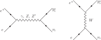
Figure 1: Feynman diagrams contributing to $e^{+}e^{-}\rightarrow\nu\bar{\nu}$

In Fig.1, the coupling between neutrinos and photon arises at the quantum level from loop diagrams. The general expression for the electromagnetic form factors of a massive neutrino is as follows Neutrino-FFactor-Kayser ; Neutrino-FFactor-Nieves ; Neutrino-FFactor-Broggini ; EMproperties-Neutrino

$$\Gamma^{\mu}(q)=eF_{1}(q^{2})\gamma^{\mu}+\frac{ie}{2m_{\nu}}F_{2}(q^{2})\sigma^{\mu\nu}q_{\nu}+\frac{e}{2m_{\nu}}F_{3}(q^{2})\gamma_{5}\sigma^{\mu\nu}q_{\nu}+eF_{4}(q^{2})\gamma_{5}\left(\gamma^{\mu}-\frac{q\hbox to0.0pt{\hss/}q^{\mu}}{q^{2}}\right),$$ (35)

where $q^{\mu}$ is the photon momentum, and $F_{i}(q^{2}),\,,\,i=1,2,3,4$ are the electromagnetic form factors of the neutrino. In this analysis, we are interested in the anomalous magnetic moment (AMM) and the electric dipole moment (EDM) of the neutrino, which are defined in terms of the $F_{2}$ and $F_{3}$ form factors at $q^{2}=0$ as follows:

$$\mu_{\nu}=\frac{m_{e}}{m_{\nu}}F_{2}|_{q^{2}=0},\hskip 14.22636ptd_{\nu}=\frac{e}{2m_{\nu}}F_{3}|_{q^{2}=0}\,.$$ (36)

III.1 Low energy amplitudes

For our purpose, the low energy limit where the propagator of gauge bosons takes a form $\frac{-ig_{\mu\nu}}{M^{2}}$ is applicable. In the mentioned limit, the amplitudes are thus given by:

$$i\mathcal{M}^{\gamma}_{fi} = \bar{u}\left(k_{2},\lambda_{4}\right)\Gamma^{\mu}v\left(k_{1},\lambda_{3}\right)\frac{g_{\mu\nu}}{\left(p_{1}+p_{2}\right)^{2}}\bar{v}\left(p_{1}\right)e\gamma^{\nu}u\left(p_{2}\right),$$ (37)

$$i\mathcal{M}^{Z}_{fi} = -\left(\frac{g^{2}}{8\cos^{2}{\theta_{W}}M_{Z}^{2}}\right)\bar{u}\left(k_{2},\lambda_{4}\right)\gamma^{\mu}\left[1-\gamma_{5}\right]v\left(k_{1},\lambda_{3}\right)$$ (38)

$$\times \bar{v}\left(p_{1}\right)\gamma_{\mu}\left[g_{V}^{Z}(e)-{g_{A}^{Z}(e)}\gamma_{5}\right]u\left(p_{2}\right)$$

$$i\mathcal{M}^{W}_{fi} = -\left(\frac{g^{2}}{8M_{W}^{2}}\right)\bar{u}\left(k_{2},\lambda_{4}\right)\gamma^{\mu}\left[1-\gamma_{5}\right]u\left(k_{1},\lambda_{3}\right)$$ (39)

$$\times \bar{v}\left(p_{1}\right)\gamma_{\mu}\left[1-\gamma_{5}\right]v\left(p_{2}\right)$$

$$i\mathcal{M}^{Z^{\prime}}_{fi} = -\left(\frac{g^{2}}{4\cos^{2}{\theta_{W}}M_{Z^{\prime}}^{2}}\right)\bar{u}\left(k_{2},\lambda_{4}\right)\gamma^{\mu}\left[g_{V}^{Z^{\prime}}(\nu)-{g_{A}^{Z^{\prime}}(\nu)}\gamma_{5}\right]v\left(k_{1},\lambda_{3}\right)$$ (40)

$$\times \bar{v}\left(p_{1}\right)\gamma_{\mu}\left[g_{V}^{Z^{\prime}}(e)-{g_{A}^{Z^{\prime}}(e)}\gamma_{5}\right]u\left(p_{2}\right)\,.$$

Using Fierz transformation generalized-Fierz and summing over (38) and (39) we have

$$i\mathcal{M}^{SM}_{fi} = -\left(\frac{g^{2}}{8\cos^{2}{\theta_{W}}M_{Z}^{2}}\right)\bar{u}\left(k_{2},\lambda_{4}\right)\gamma^{\mu}\left[1-\gamma_{5}\right]v\left(k_{1},\lambda_{3}\right)$$ (41)

$$\times \bar{v}\left(p_{1}\right)\gamma_{\mu}\left[C_{V}(e)-C_{A}(e)\gamma_{5}\right]u\left(p_{2}\right)$$

where $C_{V}(e)=1+g_{V}^{Z}(e)=\frac{1}{2}+2\sin^{2}{\theta_{W}}$ and $C_{A}(e)=1+g_{A}^{Z}(e)=\frac{1}{2}$.

The final amplitude is

$$\mathcal{M}_{fi}^{331\beta}=\mathcal{M}_{fi}^{SM}+\mathcal{M}_{fi}^{\gamma}+\mathcal{M}_{fi}^{Z^{\prime}}\,.$$ (42)

Squaring (42), summing and and taking average over spin of particles in the final and initial states, respectively, we get:

$$\frac{1}{4}\sum_{s}\left|\mathcal{M}_{fi}\right|^{2}=\frac{\left(4\pi\alpha\right)^{2}}{\sin^{4}{2\theta_{W}}}\Bigg{\{}\frac{\sin^{4}{2\theta_{W}}}{\left(4\pi\alpha\right)}(\mu_{\nu}^{2}+d_{\nu}^{2})\Big{[}\frac{(p_{1}\cdot p_{2}+m_{e}^{2})(p_{1}\cdot k_{2}+m_{e}^{2})}{s}\Big{]}$$

$$+\Bigg{[}\bigg{(}\frac{1}{M_{Z}^{2}}\big{[}C_{V}(e)-C_{A}(e)\big{]}+\frac{1}{M_{Z^{\prime}}^{2}}\big{[}g_{V}^{Z^{\prime}}(e)-g_{A}^{Z^{\prime}}(e)\big{]}\big{[}g_{V}^{Z^{\prime}}(\nu)+g_{A}^{Z^{\prime}}(\nu)\big{]}\bigg{)}^{2}$$

$$+\bigg{(}\frac{1}{M_{Z^{\prime}}^{2}}\big{[}g_{V}^{Z^{\prime}}(e)+g_{A}^{Z^{\prime}}(e)\big{]}\big{[}g_{V}^{Z^{\prime}}(\nu)-g_{A}^{Z^{\prime}}(\nu)\big{]}\bigg{)}^{2}\Bigg{]}\times\left(p_{1}\cdot k_{1}\right)\left(p_{2}\cdot k_{2}\right)$$

$$+\Bigg{[}\bigg{(}\frac{1}{M_{Z}^{2}}\big{[}C_{V}(e)+C_{A}(e)\big{]}+\frac{1}{M_{Z^{\prime}}^{2}}\big{[}g_{V}^{Z^{\prime}}(e)+g_{A}^{Z^{\prime}}(e)\big{]}\big{[}g_{V}^{Z^{\prime}}(\nu)+g_{A}^{Z^{\prime}}(\nu)\big{]}\bigg{)}^{2}$$

$$+\bigg{(}\frac{1}{M_{Z^{\prime}}^{2}}\big{[}g_{V}^{Z^{\prime}}(e)-g_{A}^{Z^{\prime}}(e)\big{]}\big{[}g_{V}^{Z^{\prime}}(\nu)-g_{A}^{Z^{\prime}}(\nu)\big{]}\bigg{)}^{2}\Bigg{]}\times\left(p_{1}\cdot k_{2}\right)\left(p_{2}\cdot k_{1}\right)$$

$$+2\Bigg{[}\frac{1}{2M_{Z}^{4}}\Big{[}\left(C_{V}(e)\right)^{2}-\left(C_{A}(e)\right)^{2}\Big{]}+\frac{1}{M_{Z^{\prime}}^{4}}\Big{[}\left(g_{V}^{Z^{\prime}}(e)\right)^{2}-\left(g_{A}^{Z^{\prime}}(e)\right)^{2}\Big{]}$$

$$\times\Big{[}\left(g_{V}^{Z^{\prime}}(\nu)\right)^{2}+\left(g_{A}^{Z^{\prime}}(\nu)\right)^{2}\Big{]}$$

$$+\frac{2}{M_{Z}^{2}M_{Z^{\prime}}^{2}}\left[C_{V}(e)g_{V}^{Z^{\prime}}(e)-C_{A}(e)g_{A}^{Z^{\prime}}(e)\right]\left[\frac{1}{2}g_{V}^{Z^{\prime}}(\nu)+\frac{1}{2}(\nu)g_{A}^{Z^{\prime}}(\nu)\right]\Bigg{]}$$

$$\times\left(m_{e}^{2}\right)\left(k_{1}\cdot k_{2}\right)\Bigg{\}}$$

(43)

Denoting new coefficients defined as follows:

$$\mathcal{C}_{1} = \Bigg{[}\bigg{(}\frac{1}{M_{Z}^{2}}\big{[}C_{V}(e)-C_{A}(e)\big{]}+\frac{1}{M_{Z^{\prime}}^{2}}\big{[}g_{V}^{Z^{\prime}}(e)-g_{A}^{Z^{\prime}}(e)\big{]}\big{[}g_{V}^{Z^{\prime}}(\nu)+g_{A}^{Z^{\prime}}(\nu)\big{]}\bigg{)}^{2}$$ (44)

$$+ \bigg{(}\frac{1}{M_{Z^{\prime}}^{2}}\big{[}g_{V}^{Z^{\prime}}(e)+g_{A}^{Z^{\prime}}(e)\big{]}\big{[}g_{V}^{Z^{\prime}}(\nu)-g_{A}^{Z^{\prime}}(\nu)\big{]}\bigg{)}^{2}\Bigg{]}$$

$$\mathcal{C}_{2} = \Bigg{[}\bigg{(}\frac{1}{M_{Z}^{2}}\big{[}C_{V}(e)+C_{A}(e)\big{]}+\frac{1}{M_{Z^{\prime}}^{2}}\big{[}g_{V}^{Z^{\prime}}(e)+g_{A}^{Z^{\prime}}(e)\big{]}\big{[}g_{V}^{Z^{\prime}}(\nu)+g_{A}^{Z^{\prime}}(\nu)\big{]}\bigg{)}^{2}$$ (45)

$$+ \bigg{(}\frac{1}{M_{Z^{\prime}}^{2}}\big{[}g_{V}^{Z^{\prime}}(e)-g_{A}^{Z^{\prime}}(e)\big{]}\big{[}g_{V}^{Z^{\prime}}(\nu)-g_{A}^{Z^{\prime}}(\nu)\big{]}\bigg{)}^{2}\Bigg{]}$$

$$\mathcal{C}_{3} = 2\Bigg{[}\frac{1}{2M_{Z}^{4}}\Big{[}\left(C_{V}(e)\right)^{2}-\left(C_{A}(e)\right)^{2}\Big{]}$$ (46)

$$+ \frac{1}{M_{Z^{\prime}}^{4}}\Big{[}\left(g_{V}^{Z^{\prime}}(e)\right)^{2}-\left(g_{A}^{Z^{\prime}}(e)\right)^{2}\Big{]}\Big{[}\left(g_{V}^{Z^{\prime}}(\nu)\right)^{2}+\left(g_{A}^{Z^{\prime}}(\nu)\right)^{2}\Big{]}$$

$$+ \frac{2}{M_{Z}^{2}M_{Z^{\prime}}^{2}}\big{[}C_{V}(e)g_{V}^{Z^{\prime}}(e)-C_{A}(e)g_{A}^{Z^{\prime}}(e)\big{]}\big{[}\frac{1}{2}g_{V}^{Z^{\prime}}(\nu)+\frac{1}{2}g_{A}^{Z^{\prime}}(\nu)\big{]}\Bigg{]}\,,$$

then Eq. (43) can be rewritten as

$$\frac{1}{4}\sum_{s}\left|\mathcal{M}_{fi}\right|^{2}=\frac{\left(4\pi\alpha\right)^{2}}{\sin^{4}{2\theta_{W}}}\Bigg{\{}\frac{\sin^{4}{2\theta_{W}}}{s\left(4\pi\alpha\right)}\left(\mu_{\nu}^{2}+d_{\nu}^{2}\right)\left[\left(p_{1}\cdot p_{2}+m_{e}^{2}\right)\left(p_{1}\cdot k_{2}+m_{e}^{2}\right)\right]$$

$$+\mathcal{C}_{1}\times\left(p_{1}\cdot k_{1}\right)\left(p_{2}\cdot k_{2}\right)+\mathcal{C}_{2}\times\left(p_{1}\cdot k_{2}\right)\left(p_{2}\cdot k_{1}\right)+\mathcal{C}_{3}\left(m_{e}^{2}\right)\left(k_{1}\cdot k_{2}\right)\Bigg{\}}\,.$$ (47)

where $s=\left(p_{1}+p_{2}\right)^{2}=\left(k_{1}+2_{2}\right)^{2}$. For future presentation, let us concrete the notations: four momentum is $p_{i}=(E_{i},\vec{p}_{i}),i=1,2$ and $k_{i}=(E_{i},\vec{k}_{i}),i=1,2$.

III.2 Stellar energy loss rates

The ionized gas in thermal equilibrium with a temperature $T$ and density $\rho$ is suggested to be exist in the star content.

Due to Fermi-Dirac distributions, the number densities of the electrons and positrons are given by

$$n_{\pm}=\int dn_{\pm}=\frac{2}{(2\pi)^{3}}\int\frac{d^{3}p}{\left(e^{\frac{E\mp\mu}{kT}}+1\right)}\,,$$ (48)

where $\mu$ is the electron chemical potential.Then, the plasma mass density is given as:

$$n_{0}=n_{-}-n_{+}=N\frac{\rho}{\mu_{e}}$$ (49)

where $N$ is Avogadro’s number.

The expression for the stellar ELRs for pair-annihilation process in (34) is determined by Dipole-Eloss-Kerimov1992 ; neutrino-Eloss-esposito2002 ; Dipole-Eloss-Heger2009 ; QSM-Dicus1972 :

$$\mathcal{Q}_{\nu\bar{\nu}}^{331\beta} =\frac{4}{\left(2\pi\right)^{6}}\int_{m_{e}}^{\infty}{\frac{d^{3}\mathbf{p}_{1}}{\left[e^{\left(E_{1}-\mu\right)/T}+1\right]}\frac{d^{3}\mathbf{p}_{2}}{\left[e^{\left(E_{2}+\mu\right)/T}+1\right]}\left(E_{1}+E_{2}\right)}v\sigma_{tot}^{331\beta},$$ (50)

$$=\frac{16}{(2\pi)^{4}}\int_{m_{e}}^{\infty}{\frac{|\mathbf{p}_{1}|E_{1}dE_{1}}{\left[e^{\left(E_{1}-\mu\right)/T}+1\right]}\frac{|\mathbf{p}_{2}|E_{2}dE_{2}}{\left[e^{\left(E_{2}+\mu\right)/T}+1\right]}\left(E_{1}+E_{2}\right)}v\sigma_{tot}^{331\beta},$$

where $\sigma_{tot}$ is the process cross-section, $\left[\exp\left({\left(E_{1,2}\pm\mu\right)/T}\right)+1\right]^{-1}$ is the Fermi-Dirac distribution functions for electron/positron, $\mu$ is the electron chemical potential, $T$ is the stellar temperature and $v$ is the electron-positron relative velocity $\frac{1}{2}[s(s-4m_{e}^{2})]^{1/2}$ .

The quantity $E_{1}E_{2}v\sigma_{tot}$ is given by Dipole-Eloss-Heger2009

$$E_{1}E_{2}v\sigma_{tot}^{331\beta} = \frac{1}{4}\int{\frac{d^{3}k_{1}d^{3}k_{2}}{\left(2\pi\right)^{3}2E_{3}\left(2\pi\right)^{3}2E_{4}}}\left|\mathcal{M}_{fi}\right|^{2}\left(2\pi\right)^{4}\delta^{4}\left(p_{1}+p_{2}-k_{1}-k_{2}\right)$$

$$= \frac{\pi\alpha^{2}}{3\sin^{4}{2\theta_{W}}}\Bigg{\{}\frac{\sin^{4}\theta_{W}}{2\pi\alpha}\left(\mu_{\nu}^{2}+d_{\nu}^{2}\right)\left(2m_{e}^{2}+p_{1}\cdot p_{2}\right)+\Big{(}\mathcal{C}_{1}^{331\beta}\Big{)}\Big{[}m_{e}^{4}$$

$$+ 3m_{e}^{2}\left(p_{1}\cdot p_{2}\right)+2\left(p_{1}\cdot p_{2}\right)^{2}\Big{]}+12\Big{(}\mathcal{C}_{2}^{331\beta}\Big{)}\Big{[}m_{e}^{4}+m_{e}^{2}\left(p_{1}\cdot p_{2}\right)\Big{]}\Bigg{\}}\,,$$

where the coefficients $\mathcal{C}_{1,2}^{331\beta}$ are defined as:

$$\mathcal{C}_{1}^{331\beta}=\dfrac{1}{2M_{Z}^{4}}\Big{[}C^{2}_{V}(e)+C^{2}_{A}(e)\Big{]}+\dfrac{1}{M_{Z^{\prime}}^{4}}\Big{[}\left(g_{V}^{Z^{\prime}}(e)\right)^{2}+\left(g_{A}^{Z^{\prime}}(e)\right)^{2}\Big{]}$$

$$\times\Big{[}\left(g_{V}^{Z^{\prime}}(\nu)\right)^{2}+\left(g_{A}^{Z^{\prime}}(\nu)\right)^{2}\Big{]}+\dfrac{1}{M_{Z}^{2}M_{Z^{\prime}}^{2}}\big{[}C_{V}(e)g_{V}^{Z^{\prime}}(e)+C_{A}(e)g_{A}^{Z^{\prime}}(e)\big{]}$$

$$\times\big{[}g_{V}^{Z^{\prime}}(\nu)+g_{A}^{Z^{\prime}}(\nu)\big{]}\,,$$

$$\mathcal{C}_{2}^{331\beta}=\dfrac{1}{2M_{Z}^{4}}\Big{[}C^{2}_{V}(e)-C^{2}_{A}(e)\Big{]}+\dfrac{1}{M_{Z^{\prime}}^{4}}\Big{[}\left(g_{V}^{Z^{\prime}}(e)\right)^{2}-\left(g_{A}^{Z^{\prime}}(e)\right)^{2}\Big{]}$$

$$\times\Big{[}\left(g_{V}^{Z^{\prime}}(\nu)\right)^{2}+\left(g_{A}^{Z^{\prime}}(\nu)\right)^{2}\Big{]}+\dfrac{1}{M_{Z}^{2}M_{Z^{\prime}}^{2}}\big{[}C_{V}(e)g_{V}^{Z^{\prime}}(e)-C_{A}(e)g_{A}^{Z^{\prime}}(e)\big{]}$$

$$\times\big{[}g_{V}^{Z^{\prime}}(\nu)+g_{A}^{Z^{\prime}}(\nu)\big{]}\,.$$ (52)

The calculation of the stellar ELRs given by (50) can be fulfill by expressing in terms of the Fermi integral defined as

$$G_{n}^{\pm}(\lambda,\eta,x)=\lambda^{{3+2n}}\int_{\lambda^{-1}}^{\infty}{x^{2n+1}\frac{\sqrt{x^{2}-\lambda^{-2}}}{\left(e^{\left(x\pm\eta\right)}+1\right)}}dx,$$ (53)

where dimensionless variables $\lambda$ and $\eta$ are defined as:

$$\lambda=\frac{k_{B}T}{m_{e}},\hskip 14.22636pt\eta=\frac{\mu_{e}}{k_{B}T}.$$ (54)

Assuming $k_{B}=1$ for the Boltzmann constant and from (48) and (49) ones have:

$$G_{s}^{\pm}(\lambda,\eta,E)=\frac{1}{m_{e}^{3+2s}}\int_{m_{e}/T}^{\infty}{E^{2s+1}\frac{\sqrt{E^{2}-m_{e}^{2}}}{\left(e^{\left(E\pm\mu_{e}\right)/T}+1\right)}}dE\,,$$ (55)

and

$$N\frac{\rho}{\mu_{e}}=\frac{m_{e}^{3}}{\pi^{2}}[G_{0}^{-}-G_{0}^{+}]\,.$$ (56)

Hence, the stellar ELRs can be expressed as:

$$\mathcal{Q}^{331\beta}=\frac{\alpha^{2}m_{e}^{9}}{9\pi^{3}\sin^{4}{2\theta_{W}}}\Bigg{\{}\frac{3\sin^{4}{2\theta_{W}}}{2\pi\alpha m_{e}^{2}}\left(\mu_{\nu}^{2}+d_{\nu}^{2}\right)$$

$$\times\bigg{[}2\Big{(}G_{-1/2}^{-}G_{0}^{+}+G_{0}^{-}G_{-1/2}^{+}\Big{)}+G_{0}^{-}G_{1/2}^{+}+G_{1/2}^{-}G_{0}^{+}\bigg{]}$$

$$+4\Big{(}\mathcal{C}_{1}^{331\beta}\Big{)}\bigg{[}5\Big{(}G_{-1/2}^{-}G_{0}^{+}+G_{0}^{-}G_{-1/2}^{+}\Big{)}+7\Big{(}G_{0}^{-}G_{1/2}^{+}+G_{1/2}^{-}G_{0}^{+}\Big{)}$$

$$-2\Big{(}G_{1}^{-}G_{-1/2}^{+}+G_{-1/2}^{-}G_{1}^{+}\Big{)}+8\Big{(}G_{1}^{-}G_{1/2}^{+}+G_{1/2}^{-}G_{1}^{+}\Big{)}\bigg{]}$$

$$+36\Big{(}\mathcal{C}_{2}^{331\beta}\Big{)}\bigg{[}G_{-1/2}^{-}G_{0}^{+}+G_{0}^{-}G_{-1/2}^{+}+G_{0}^{-}G_{1/2}^{+}+G_{1/2}^{-}G_{0}^{+}\bigg{]}\Bigg{\}}.$$ (57)

To investigate the effects of dipole moments and new contribution of $Z^{\prime}$ boson on the ELR we have to evaluate the relative correction for the star ELR between 3-3-1$\beta$ model and that of the SM ($\mathcal{Q}^{SM}$) QSM-Dicus1972 given as:

$$\mathcal{Q}^{SM}=\frac{G_{F}^{2}m_{e}^{9}}{18\pi}\Biggl{\{}(7C_{V}(e)^{2}-2C_{A}(e)^{2})[G_{0}^{-}G_{1/2}^{+}+G_{-1/2}^{-}G_{0}^{+}]$$

$$+9C_{V}(e)^{2}[G_{1/2}^{-}G_{0}^{+}+G_{0}^{-}G_{1/2}^{+}]+(C_{V}(e)^{2}+C_{A}(e)^{2})[4G_{1}^{-}G_{1/2}^{+}+G_{1/2}^{-}G_{1}^{+}$$

$$-G_{1}^{-}G_{-1/2}^{+}-G_{1/2}^{-}G_{0}^{+}-G_{0}^{-}G_{1/2}^{+}-G_{-1/2}^{-}G_{1}^{+}]\Biggr{\}}\,,$$ (58)

Hence

$$\frac{\delta\mathcal{Q}^{331\beta}}{\mathcal{Q}^{SM}}=\frac{\mathcal{Q}^{331\beta}\left(\mu_{\nu},d_{\nu},\beta,M_{Z^{\prime}},\eta\right)-\mathcal{Q}^{SM}\left(\eta\right)}{\mathcal{Q}^{SM}\left(\eta\right)}.$$ (59)

Since the functions $G^{\pm}(\lambda,\eta)$ can only be defined analytically in some limiting regions of parameters $\lambda$ and $\eta$ therefore we will investigate the correction (59) in five regions

III.2.1 Region I: $\lambda\ll 1$ and $\eta\ll 1/\lambda$

In this region, temperature and densities vary between $3\times 10^{8}\,\textrm{K}\leq\textrm{T}\leq 3\times 10^{9}\,\textrm{K}$ and $\rho\leq 10^{5}gr/cm^{3}$, respectively.

The Fermi integral is

$$G_{n}^{\pm}(\lambda,\eta,x)=\lambda^{{3+2n}}\int_{\lambda^{-1}}^{\infty}{x^{2n+1}\frac{\sqrt{x^{2}-\lambda^{-2}}}{\left(e^{\left(x\pm\eta\right)}+1\right)}}dx\,.$$ (60)

Changing variable $x=z+\lambda^{-1}$ yields

$$G_{n}^{\pm}=\sqrt{2}\lambda^{3/2}e^{-\lambda^{-1}}e^{\mp\eta}\int_{0}^{\infty}dz(\lambda z+1)^{2n+1}z^{1/2}\left(1+\frac{\lambda z}{2}\right)^{1/2}e^{-z}$$ (61)

For every $\lambda$ satisfying $\lambda z\approx\epsilon$ we have

$$(\lambda z+1)^{2n+1}\hskip 14.22636pt[1+(2n+1)\lambda z],\hskip 14.22636pt\left(1+\frac{\lambda z}{2}\right)^{1/2}\approx 1+\frac{\lambda z}{4}$$

Neglecting the second order in $\lambda z$ ones get

$$G_{n}^{\pm} =\sqrt{2}\lambda^{3/2}e^{-\lambda^{-1}}e^{\mp\eta}\left[\int_{0}^{\infty}dzz^{1/2}e^{-z}+\left(2n+\frac{5}{4}\right)\lambda\int_{0}^{\infty}dzz^{3/2}e^{-z}\right]$$ (62)

$$=\sqrt{2}\lambda^{3/2}e^{-\lambda^{-1}}e^{\mp\eta}\left[\Gamma(3/2)+\left(2n+\frac{5}{4}\lambda\right)\Gamma(5/2)\right]$$

$$=\sqrt{\frac{\pi}{2}}\lambda^{3/2}e^{-\lambda^{-1}}e^{\mp\eta}\left[1+\frac{3}{2}\left(2n+\frac{5}{4}\right)\lambda\right]\,,$$

where $\Gamma(n)=\int_{0}^{\infty}z^{n-1}e^{-z}dz$.

In the case $1\ll\lambda^{-1}$ ones have

$$G_{0}^{\pm}\approx\sqrt{\frac{\pi}{2}}\lambda^{3/2}e^{-\lambda^{-1}}e^{\mp\eta}$$ (63)

and

$$G_{n}^{-}\approx G_{0}^{-}=\left(\frac{\pi}{2}\right)^{\frac{1}{2}}\lambda^{\frac{3}{2}}e^{-1/\lambda}e^{\eta}.$$ (64)

Hence, we get

$$\mathcal{Q}_{I}^{331\beta} =\frac{\alpha^{2}m_{e}^{9}}{\pi^{3}\sin^{4}{2\theta_{W}}}\Bigg{[}\frac{\sin^{4}{2\theta_{W}}}{\pi\alpha m_{e}^{2}}\left(\mu_{\nu}^{2}+d_{\nu}^{2}\right)+16(\mathcal{C}_{1}^{331\beta}+\mathcal{C}_{2}^{331\beta})\Bigg{]}G_{0}^{-}G_{0}^{+}$$ (65)

$$=\frac{\alpha^{2}m_{e}^{9}}{\pi^{3}\sin^{4}{2\theta_{W}}}\Bigg{[}\frac{\sin^{4}{2\theta_{W}}}{\pi\alpha m_{e}^{2}}\left(\mu_{\nu}^{2}+d_{\nu}^{2}\right)+16(\mathcal{C}_{1}^{331\beta}+\mathcal{C}_{2}^{331\beta})\Bigg{]}$$

$$\times\left(\frac{\pi}{2}\right)^{3/2}\left(\frac{T}{m_{e}}\right)^{3}e^{-2m_{e}/T}$$

and

$$\mathcal{Q}_{I}^{SM} =\frac{G_{F}^{2}m_{e}^{9}}{18\pi^{5}}\times 36C^{2}_{V}(e)G_{0}^{-}G_{0}^{+}$$ (66)

$$=\frac{\alpha^{2}m_{e}^{9}}{\pi^{3}\sin^{4}{2\theta_{W}}}\frac{16}{m_{Z}^{4}}C_{V}^{2}(e)G_{0}^{-}G_{0}^{+}$$

Then, the correction is given by:

$$\frac{\delta\mathcal{Q}_{I}^{331\beta}}{\mathcal{Q}_{I}^{SM}}=\frac{\Bigg{[}\frac{\sin^{4}{2\theta_{W}}}{\pi\alpha m_{e}^{2}}\left(\mu_{\nu}^{2}+d_{\nu}^{2}\right)+16(\mathcal{C}_{1}^{331\beta}+\mathcal{C}_{2}^{331\beta})\Bigg{]}-\frac{16}{m_{Z}^{4}}C_{V}^{2}(e)}{\frac{16}{m_{Z}^{4}}C_{V}^{2}(e)}$$ (67)

III.2.2 Region II: $\lambda\ll 1$ and $\frac{1}{\lambda}\ll\eta\ll\frac{2}{\lambda}$

This region is nonrelativistic and mildly degenerate, with temperatures $T\leq 10^{8}$ K and densities between $10^{4}gr/cm^{3}\,\leq\rho\leq\,10^{6}gr/cm^{3}$.

The Fermi integrals satisfy the following conditions QBSM-Hernandez ; QBSM-Hernandez ; QSM-Dicus1972 : $G_{0}^{-}\gg G_{0}^{+}$ and $G_{n}^{-}\approx G_{0}^{-}$ and

$$G_{n}^{+}\approx G_{0}^{+}=\left(\frac{\pi}{2}\right)^{\frac{1}{2}}\lambda^{\frac{3}{2}}e^{-1/\lambda}e^{-\eta},\qquad G_{n}^{-}\approx G_{0}^{-}=\left(\frac{\rho}{\mu_{e}}\right)\frac{\pi^{2}}{m_{e}^{3}}N_{A}.$$ (68)

Then ones have:

$$\mathcal{Q}_{II}^{331\beta} =\frac{\alpha^{2}m_{e}^{9}}{\pi^{3}\sin^{4}{2\theta_{W}}}\Bigg{[}\frac{\sin^{4}{2\theta_{W}}}{\pi\alpha m_{e}^{2}}\left(\mu_{\nu}^{2}+d_{\nu}^{2}\right)+16(\mathcal{C}_{1}^{331\beta}+\mathcal{C}_{2}^{331\beta})\Bigg{]}G_{0}^{-}G_{0}^{+}$$ (69)

$$=\frac{\alpha^{2}m_{e}^{6}}{\pi\sin^{4}{2\theta_{W}}}\left(\frac{\rho}{\mu_{e}}N_{A}\right)\left(\frac{\pi}{2}\right)^{1/2}\left(\frac{T}{m_{e}}\right)^{3/2}e^{-(m_{e}+\mu_{e})/T}$$

$$\times\Bigg{[}\frac{\sin^{4}{2\theta_{W}}}{\pi\alpha m_{e}^{2}}\left(\mu_{\nu}^{2}+d_{\nu}^{2}\right)+16(\mathcal{C}_{1}^{331\beta}+\mathcal{C}_{2}^{331\beta})\Bigg{]}$$

and

$$\mathcal{Q}_{II}^{SM} =\frac{G_{F}^{2}m_{e}^{9}}{18\pi^{5}}\times 36C^{2}_{V}(e)G_{0}^{-}G_{0}^{+}$$ (70)

$$=\frac{\alpha^{2}m_{e}^{9}}{\pi^{3}\sin^{4}{2\theta_{W}}}\frac{16}{m_{Z}^{4}}C_{V}^{2}(e)G_{0}^{-}G_{0}^{+}$$

$$=\frac{\alpha^{2}m_{e}^{9}}{\pi^{3}\sin^{4}{2\theta_{W}}}\frac{16}{m_{Z}^{4}}C_{V}^{2}(e)\left(\frac{\rho}{\mu_{e}}N_{A}\frac{\pi^{2}}{m_{e}^{3}}\right)\left(\frac{\pi}{2}\right)^{1/2}\left(\frac{T}{m_{e}}\right)^{3/2}e^{-(m_{e}+\mu_{e})/T}\,.$$

Therefore the correction is given as exactly as in (67) which is equal as in region I.

III.2.3 Region III: $\lambda\ll 1$ and  $1\ll\lambda\eta$

The considered region represents the relativistic and degenerate case and is valid for temperatures $T>6\times 10^{7}$ K and densities $\rho>10^{7}gr/cm^{3}$. The Fermi integrals result:

$$G_{n}^{+}\approx G_{0}^{+}=\left(\frac{\pi}{2}\right)^{\frac{1}{2}}\lambda^{\frac{3}{2}}e^{-1/\lambda}e^{-\eta},\hskip 14.22636ptG_{n}^{-}=\left(\frac{3}{2n+3}\right)\left(\lambda\eta\right)^{2n}G_{0}^{-}.$$ (71)

Then to highest power in $\lambda\eta$ ones have

$$\mathcal{Q}_{III}^{331\beta} =\frac{8\alpha^{2}m_{e}^{9}}{3\pi^{3}\sin^{4}{2\theta_{W}}}\mathcal{C}_{1}^{331\beta}G_{1}^{-}G_{0}^{+}$$ (72)

$$=\frac{8\alpha^{2}m_{e}^{9}}{3\pi^{3}\sin^{4}{2\theta_{W}}}\frac{3}{5}\left(\frac{1}{m_{e}}\frac{\mu_{e}}{T}\right)^{2}\left(\frac{\rho}{\mu_{e}}\right)\frac{\pi^{2}}{\mu^{3}_{e}}N_{A}\left(\frac{\pi}{2}\right)^{1/2}\left(\frac{T}{m_{e}}\right)^{3/2}$$

$$\times e^{-({m_{e}+\mu_{e}})/{T}}\mathcal{C}_{1}^{331\beta},$$

and

$$\mathcal{Q}^{SM}=\frac{4}{3}\frac{\alpha^{2}m_{e}^{9}}{\pi^{3}\sin^{4}{2\theta_{W}}m^{4}_{Z}}[C_{V}^{2}(e)+C^{2}_{A}(e)]G_{1}^{-}G_{0}^{+}\,.$$ (73)

The relativistic correction is given by:

$$\frac{\delta\mathcal{Q}^{331\beta}_{III}}{\mathcal{Q}^{SM}_{III}} = \frac{2m^{4}_{Z}\mathcal{C}_{1}^{331\beta}}{[C_{V}^{2}(e)+C^{2}_{A}(e)]}-1\,.$$ (74)

Since the approximation for this region only considers the terms of dominant powers, so there is no dependence on the AMM and/or EDM of the neutrino.

III.2.4 Region IV: $\lambda\gg 1$ and $\eta\ll 1$

The relativistic and nondegenerate case holds for densities $\rho>10^{7}gr/cm^{3}$. In this region we may ignore the chemical potential. Considering the dominance of the highest orders in $\lambda$, we get

$$G_{n}^{\pm}\approx\lambda^{2n+3}\Gamma\left(2n+3\right)\sum_{S=1}^{\infty}\frac{\left(-1\right)^{S+1}}{S^{2n+3}}.$$ (75)

Then, the stellar ELRs for this region is given by

$$\mathcal{Q}_{IV}^{331\beta} =\frac{64\alpha^{2}m_{e}^{9}}{9\pi^{3}\sin^{4}{2\theta_{W}}}\mathcal{C}_{1}^{331\beta}G_{1}^{-}G_{1/2}^{+}$$ (76)

$$=\frac{64\alpha^{2}m_{e}^{9}}{9\pi^{3}\sin^{4}{2\theta_{W}}}\mathcal{C}_{1}^{331\beta}\left(\frac{T}{m_{e}}\right)^{9}\Gamma(5)\xi(5)\Gamma(4)\xi(4)$$

where $\Gamma$ and $\xi$ are the Gamma and Riemann zeta functions, respectively.

For the SM the ELR is given by:

$$\mathcal{Q}^{SM}=\frac{32\alpha^{2}m_{e}^{9}}{9\pi^{3}\sin^{4}{2\theta_{W}}m^{4}_{Z}}(C^{2}_{V}(e)+C^{2}_{A}(e))G_{1}^{-}G_{1/2}^{+}\,.$$ (77)

Thus the relativistic correction is the same as in the previous region, namely

$$\frac{\delta\mathcal{Q}^{331\beta}_{IV}}{\mathcal{Q}^{SM}_{IV}} = \frac{2m_{Z}^{4}\mathcal{C}_{1}^{331\beta}}{[C_{V}^{2}(e)+C^{2}_{A}(e)]}-1.$$ (78)

III.2.5 Region V: $\lambda\gg 1$ and $\eta\gg 1$

This degenerate relativistic region holds for densities greater than $\rho>10^{8}gr/cm^{3}$ with temperatures of $T\approx 10^{10}$ K at the lowest density, extendable to a range between $10^{10}$ K and $10^{11}$ K at a density of $\rho>10^{10}gr/cm^{3}$. Here $G_{n}^{-}\gg G_{n}^{+}$, then

$$G_{n}^{+}\approx\lambda^{2n+3}\left(2n+2\right)!e^{-\eta}\hskip 14.22636ptG_{n}^{-}\approx\left(\frac{3}{2n+3}\right)\left(\lambda\eta\right)^{2n}\left(\frac{\rho}{\mu_{e}}\right)\frac{\pi^{2}}{m_{e}^{3}}N_{A}.$$ (79)

Restricting the calculation to the higher powers in $\lambda\eta$, the stellar ELRs result:

$$\mathcal{Q}^{331\beta}_{V} =\frac{32\alpha^{2}m_{e}^{9}}{9\pi^{3}\sin^{4}{2\theta_{W}}}\mathcal{C}_{1}^{331\beta}G_{1}^{-}G_{1/2}^{+}$$ (80)

$$=\frac{64\alpha^{2}m_{e}^{6}}{5\pi\sin^{4}{2\theta_{W}}}\mathcal{C}_{1}^{331\beta}\left(\frac{\rho}{\mu_{e}}N_{A}\right)\left(\frac{T}{m_{e}}\right)^{6}\left(\frac{\mu_{e}}{T}\right)^{2}e^{-\mu_{e}/{T}}$$

and

$$\mathcal{Q}^{SM}_{V} =\frac{32\alpha^{2}m_{e}^{9}}{9\pi^{3}\sin^{4}{2\theta_{W}}m_{Z}^{4}}[C_{V}^{2}(e)+C_{A}^{2}(e)]G_{1}^{-}G_{1/2}^{+}$$

and the relativistic correction is given by

$$\frac{\delta\mathcal{Q}^{331\beta}_{V}}{\mathcal{Q}^{SM}_{V}} = \frac{2m_{Z}^{4}\mathcal{C}_{1}^{331\beta}}{[C_{V}^{2}(e)+C^{2}_{A}(e)]}-1\,.$$ (82)

The above result is equal to that in Region III. Again, it becomes clear that there is an indistinguishability of treating with nondegenerate or degenerate electrons.

IV Numerical analysis

Let us investigate the pair annihilation neutrino ELR in the context of the $SU(3)_{C}\times SU(3)_{L}\times U(1)_{X}$ models. The process in (34) is one of the main mechanisms of neutrino pair production relevant for the neutrino luminosity. We investigate for both degenerate and nondegenerate Fermi gas. In the context of beyond Standard Model, at loop level the non-vanishing of AMM and EDM of neutrinos and the appearance of new neural gauge bosons with V-A interaction can contribute to the process of energy loss.

Before investigate the effect of temperature and densities on the ELR we will investigate the rate of correction of 3-3-1 models compared with the SM because with the same value of temperature and densities the parameters that distinguish models is the value of parameter of the model (the parameter $\beta$) and the mass of the new gauge bosons $m_{Z^{\prime}}$. We plot the $\mathcal{Q}$ correction for regions I, II in Figs.2 and 3. and for regions II, IV, V in Figs.4 and 5

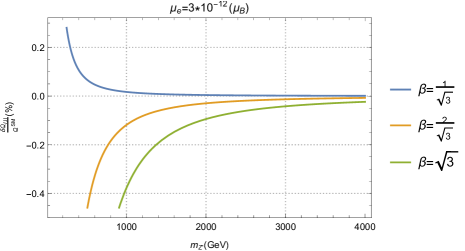
Figure 2: Q correction regions I,II with $\beta>0$

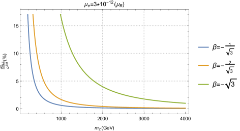
Figure 3: Q correction regions I,II with $\beta<0$

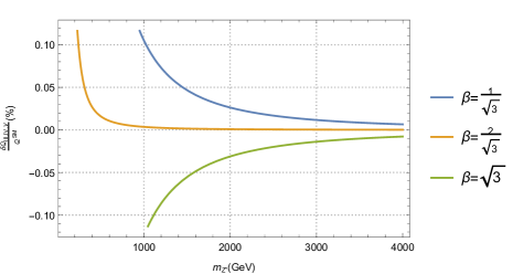
Figure 4: Q correction regions III,IV,V with $\beta>0$

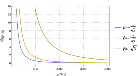
Figure 5: Q correction regions III,IV,V with $\beta<0$

The correction is plotted for all values of parameter $\beta$. For negative value of $\beta$ the correction is up to $15\%$ while positive value of $\beta$ give very small correction ($0.2\%$). For all negative $\beta$, the correction decreases with the increase of the mass of Z’ boson. For $\beta=-\frac{1}{\sqrt{3}},-\frac{2}{\sqrt{3}}$, the correction is approximated to 0% when $m_{Z^{\prime}}\geq 2000$ GeV and only increase significantly when $m_{Z^{\prime}}\approx 200$ GeV which is around the energy region of the $Z$ boson. In the case $\beta=-\sqrt{3}$, the correction is higher from 1% up to 15% in the mass range from 4000 GeV to 1000 GeV. This case is more interesting when showing that the contribution of the $Z^{\prime}$ boson in the 3-3-1 model is distinguishable with the SM. Therefore put constraints on the mass range of the $Z^{\prime}$ boson which is in agreement with searching mass range for the $Z^{\prime}$ boson at LHC PDG2016 ; Z' resonance . In the followings detail numerical analysis, we will work with the case where $\beta=-\sqrt{3}$.

In Fig.6, we plot the energy loss as a function of $M_{Z^{\prime}}$ and compare it with those in the SM. The value of temperature is set $T=3*10^{9}$K and $\mu_{\nu}=3*10^{-12}(\mu_{B})$. We plot the contribution of dipole moment and gauge boson $Z^{\prime}$ separately. In Fig.7 we plot the energy loss rate as a function of magnetic moment.

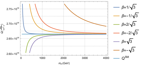
Figure 6: Energy loss rate for region I as a function of $m_{Z^{\prime}}$

Figure 7: Energy loss rate for region I as a function of magnetic dipole moment

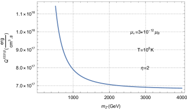
Figure 8: Energy loss rate for region II as a function of $m_{Z^{\prime}}$

To investigate the effect of only of the dipole moment we take the limit where the value of $m_{Z^{\prime}}$ very large ($\infty$). In this limit the contribution of the gauge boson $Z^{\prime}$ is small. The magnitude of $\mathcal{Q}$ increase with the value of $\mu_{\nu}$, however with current bound $\mu_{\nu}<3*10^{-12}\mu_{B}$ the value of $\mathcal{Q}<2.6675*10^{18}$ which is approximate the magnitude of those in the SM as in Fig.6 or the $\mathcal{Q}$ correction for region I-II is less than 0.1%( Fig.9) comparing with 14% of the combine contribution of both dipole moment and the $Z^{\prime}$ boson. Hence the effect of dipole moment is not clear in this case.

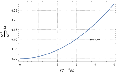
Figure 9: Energy loss rate for region I as a function of magnetic dipole moment

The Fig.10 is the case for $\mu_{\nu}=0,d_{\nu}=0$ and the value of temperature $T=3*10^{9}$ K. Plot $\mathcal{Q}$ as function of $m_{Z^{\prime}}$, for mass range of $m_{Z^{\prime}}<2000$ GeV the magnitude of energy loss $\mathcal{Q}\approx 2.8*10^{18}$ therefore the effect of gauge boson $Z^{\prime}$ is much stronger than that of dipole moment.

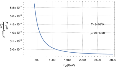
Figure 10: Energy loss rate for region I as a function of $m_{Z^{\prime}}$, for $\mu_{\nu}=0,d_{\nu}=0$, $T=3*10^{9}$ K

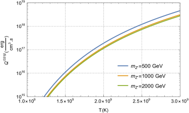
Figure 11: Energy loss rate for region I as a function of temperature

Next we plot the dependence of the energy loss on the temperature as in Fig. 11. We plot for three values of the mass of the gauge boson $m_{Z^{\prime}}=500,100,2000$ GeV. The ELR increases with the increase of the temperature. The dependence of $\mathcal{Q}$ on dimensionless parameter $\eta$ is depicted as in Fig. 12. As in the figure, $\mathcal{Q}$ decreases with the increase of $\eta$. This is what one would expect since $\eta=\frac{\mu_{e}}{k_{B}T}$ is inverse proportional to the temperature T. The dependence of $\mathcal{Q}$ on the temperature and density are plotted in Fig.13. $\mathcal{Q}$ increases in the region of high temperature and high density.

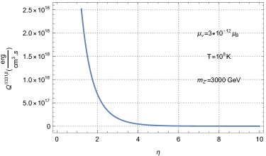
Figure 12: Energy loss rate for region II as a function of $\eta$

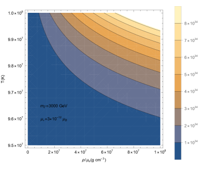
Figure 13: Energy loss rate for region II as a function of temperature and density

V Conclusions

Quantifying stellar loss energy is a priority in astrophysics and cosmology. One of most interesting possibilities is to use stars and its physical process to put set constraints on physics beyond Standard Model.

We have evaluated the stellar ELR in the frameworks of the 3-3-1$\beta$ model. The energy loss rate is in the form of neutrino emission assessed in the pair annihilation $e^{+}e^{-}\xrightarrow{\gamma,W,Z,Z^{\prime}}\nu\bar{\nu}$. We obtained the approximated formula for energy loss ($\mathcal{Q}$) and the correction $\mathcal{Q}$ in comparing with that of the SM.

We evaluated the $\mathcal{Q}$ correction for different value of $\beta=\pm\frac{1}{\sqrt{3}},\pm\frac{2}{\sqrt{3}},\pm\sqrt{3}$. The negative value of $\beta$ give higher value compared with positive value and up to 14%. We have shown that the contribution of dipole moment is small compared with that of the $Z^{\prime}$ boson. The $\mathcal{Q}$ gives the constraints on the mass range of the $Z^{\prime}$ boson $m_{Z^{\prime}}\leq 4000$ GeV which is in agreement with current searching the mass range of the $Z^{\prime}$ at LHC.

References

(1)G. G. Raffelt, Ann. Rev. Nucl. Part. Sci. 49 (1999) 163-216, arXiv:hep-ph/9903472.
(2)G. G. Raffelt, Nucl. Phys. Proc. Suppl. 72 (1999) 43-53
(3)G. Beaudet, V. Petrosian, and E. E. Salpeter, ApJ, 150, 979 (1967)
(4) S. Esposito, G. Mangano, G. Miele, I. Picardi, and O. Pisanti, Mod. Phys. Lett. A17, 491 (2002).
(5) S. Esposito, G. Mangano, G. Miele, I. Picardi, and O. Pisanti, Nucl. Phys. B658, 217 (2003).
(6)G. Gamow, Rev. Mod. Phys. 21, 367 (1949)
(7)G. Gamow, Phys. Rev. Lett. 19, 759 (1967)
(8)B. Pontecorvo, Sov. Phys. JETP 26, 984 (1968)
(9)Chris L. Fryer et al. 2002 ApJ 565 430
(10)B. P. Abbott et al., Phys. Rev. Lett. 119, 161101 (2017).
(11)T. Hatsuda, M. Yoshimura, Phys. Lett. B 203 (1988) 469-473.
(12)C. Dessert, J. W. Foster, B. R. Safdi, Phys. Rev. Lett. 125, 261102 (2020),arXiv:2008.03305.
(13)Y. Bai, Y. Hamada, Phys. Lett. B 781 (2018) 187-194, arXiv:1709.10516.
(14)S. L. Glashow, Nucl. Phys. 22, 579 (1961)
(15)S. Weinberg, Phys. Rev. Lett. 19, 1264 (1967)
(16)A. Salam, in Elementary Particle Theory: Relativistic Groups and
Analyticity (Nobel Symposium No. 8), edited by N. Svartholm (Almqvist and Wiksell, Stockholm, 1968) p. 367
(17) SNO Collab., Q. R. Ahmad et al., Phys. Rev. Lett.87
(18) SK Collab., Y. Fukuda, et al., Phys. Rev. Lett. 81
(19) A. Heger, A. Friedland, M. Giannotti, and V. Cirigliano, Astrophys. J.696, 608 (2009).
(20) B. Kerimov, S. Zeinalov, V. Alizade, and A. Mourao, Phys. Lett. B274, 477 (1992).
(21)M. A. Hernández-Ruíz, A. Gutiérrez-Rodríguez, A. González-Sánchez, Eur. Phys. J. A 53, 16 (2017).
(22) A. Llamas-Bugarín,, A. Gutiérrez-Rodríguez, A. González-Sánchez, Eur. Phys. J. Plus 135, 481 (2020).
(23) G. Senjanovic, Nucl. Phys.B 153, 334 (1979).
(24) G. Senjanovic and R. N. Mohapatra, Phys. Rev.D 12, 1502 (1975).
(25) U. Baur et al., Phys. Rev.D 35, 297 (1987).
(26) F. Pisano and V. Pleitez, Phys. Rev. D 46, 410 (1992).
(27) P. H. Frampton, Phys. Rev. Lett. 69,
2889 (1992)
(28) R. Foot et al, Phys. Rev. D 47, 4158 (1993).
(29) M. Singer, J. W. F. Valle and J. Schechter, Phys.
Rev. D 22, 738 (1980).
(30) R. Foot, H. N. Long and Tuan A.
Tran, Phys. Rev. D 50, 34 (R)(1994) [arXiv:hep-ph/9402243].
(31) J. C. Montero, F. Pisano and V. Pleitez, Phys. Rev. D 47,
2918 (1993).
(32) H. N. Long, Phys. Rev. D 54, 4691 (1996).
(33)H.N. Long, Phys. Rev. D 53, 437 (1996).
(34)R. A. Diaz, R. Martinez, F. Ochoa, Phys. Rev. D 72 (2005) 035018, arXiv:hep-ph/0411263.
(35)R. A. Diaz, R. Martinez, F. Ochoa, Phys. Rev. D 69 (2005) 095009, arXiv:hep-ph/0309280.
(36)R. A. Carcamo, R. Martinez, F. Ochoa, Phys. Rev. D 73 (2006) 035007.
(37)
A. J. Buras, F. De Fazio and J. Girrbach,
JHEP 02, 116 (2013),
arXiv:1211.1896.
(38) R. D. Peccei and H. R. Quinn, Phys. Rev. Lett. 38, 1440 (1977).
(39) P. B. Pal, Phys. Rev. D 52 (1995) 1659, [hep-ph/9411406].
(40) C. A. de S. Pires, O. P. Ravinez, Phys. Rev. D 58, 035008 (1998).
(41)
A. Doff, F. Pisano, Mod. Phys.
Lett. A 14, 1133 (1999); Phys. Rev. D 63, 097903 (2001).
(42)P. V. Dong,
H. N. Long, Int. J. Mod. Phys. A 21, 6677 (2006), arXiv:hep-ph/0507155].
(43) D. A. Dicus, Phys. Rev. D6, 941 (1972).
(44) B. Kayser and A. S. Goldhaber, Phys. Rev. D 28, 2341 (1983)
(45)J. F. Nieves, Phys. Rev. D 26, 3152 (1982).
(46)C. Broggini, C. Giunti, A. Studenikin, Advances in High Energy Physics, 2012 459526, (2012).