Quantum surface effects in strong coupling dynamics

Abstract

Plasmons in nanostructured metals are widely utilized to trigger strong light–matter interactions with quantum light sources. While the nonclassical behavior of such quantum emitters (QEs) is well-understood in this context, the role of quantum and surface effects in the plasmonic resonator is usually neglected. Here, we combine the Green’s tensor approach with the Feibelman $d$-parameter formalism to theoretically explore the influence of quantum surface effects in metal-dielectric layered nanostructures on the relaxation dynamics of a proximal two-level QE. Having identified electron spill-out as the dominant source of quantum effects in jellium-like metals, we focus our study on sodium. Our results reveal a clear splitting in the emission spectrum, indicative of having reached the strong-coupling regime, and, more importantly, non-Markovian relaxation dynamics of the emitter. Our findings establish that strong light–matter coupling is not suppressed by the emergence of nonclassical surface effects in the optical response of the metal.

Introduction — Confining light in sub-diffraction volumes via surface plasmon polaritons (SPPs) has become common practice to enhance nanoscale light–matter interactions in the past decade ozbay_sci311 . In combination with multi-level quantum emitters (QEs), plasmonic nanostructures play the role of the cavity torma_rpp78 ; Pelton_natphot ; bozhevolnyi_natphot2017 ; baumberg_natmat2019 in cavity quantum electrodynamics (QED) Mandel_Cambridge1995 ; Scully_Cambridge1997 , while the QEs, depending on the desired functionality, can be natural (atoms, molecules) or artificial (quantum wells and dots, defects in nanodiamonds, collective states in transition metal dichalcogenides or hexagonal boron nitride) akimov_nat450 ; chang_natphys3 ; goban_natcom5 ; hood_pnas113 ; fernandez_acsphot5 ; koperski_pnas117 . Advanced fabrication techniques now enable the engineering of metal cavities with characteristic dimensions below $10$ nm, as well as precise positioning of QEs within them, to produce promising templates for bright single-photon emitters manolatou_ieeejqe44 ; akselrod_natphot8 ; rose_nl14 ; chikkaraddy_nat535 ; May2020 . The plasmonic cavity is typically formed by a metallic substrate interacting with another metallic film or with dropcasted nanoparticles; separating the two plasmonic components by a thin dielectric spacer containing QEs in the form of defects, molecules, or quantum dots bogdanov_nl18 ; katzen_acsami12 ; ojambati_acsphot7 ; Ding_nanophotonics , the resulting intense electromagnetic (EM) fields, confined within minimized volumes, trigger extreme light–matter interactions.

Traditionally, in the local-response approximation (LRA) Hohenester_Springer2020 , the optical response of metals is described through the Drude model, or through experimentally measured bulk permittivities. But, as plasmonic cavities become narrower, the interaction strengths with the therein confined QEs are overestimated by LRA, as compared to experimental results ciraci_sci337 ; savage_nat491 ; scholl_nat483 , calling for amendment of the theoretical models romero_oex14 ; esteban_natcom3 ; luo_prl111 ; raza_nanophot2 ; yang_nat576 ; the main missing element is information about quantum effects in the metal. As a first extension of LRA, the hydrodynamic Drude model (HDM), which describes the motion of the compressible free-electron gas as a convective fluid, has met with considerable success moreau_prb87 ; raza_prb88 ; mortensen_natcom5 ; tserkezis_acsphot5b , yet effects associated with electron spill-out still require a self-consistent treatment toscano_natcom6 ; yan_prb2015 ; ciraci_prb93 ; ciraci2019 . However, the ultimate goal of an ab initio optical response calculation for structures with sizes of order $100$ nm at room temperature remains out of computational reach varas_nanophot5 .

A more efficient approach is based on the work of Feibelman feibelman_pss12 , who bridged EM and ab initio calculations through appropriate surface-response functions, the $d$-parameters ($d_{\perp}$ and $d_{\parallel}$), which need be calculated only once for a given surface to be implemented in a quantum-informed surface-response formalism (SRF) yan_PRL2015 ; christensen_prl118 ; yang_nat576 ; Goncalves_natcom11 ; Mortensen2021 . The full QED problem is then described by quantum-corrected mesoscopic boundary conditions at the metal surface yan_PRL2015 ; yang_nat576 . Macroscopic QED Rivera2020 ; Head-Marsden2020 allows to directly apply the rigorous Green’s function approach developed within LRA, now corrected by SRF, without invoking quantum effects in a quasi-normal mode formalism Lalanne_lpr2018 ; Dezfouli_optica2017 ; Franke_PRL2019 .

The relaxation process of a QE placed in a nanostructured environment has been extensively investigated in the context of the macroscopic QED theory. The photonic environment provides an enhanced density of optical states —often, but not restrictively, in the form of an optical resonance— at a specific energy that, when matched with the transition energy of the QE, leads to considerable QE–environment light–matter coupling-strength enhancement. Usually, the interaction is described within a Lorentzian model of the spectral density which, under strong-coupling conditions, results in a Rabi splitting in the emission spectrum and oscillations in the relaxation dynamics of the QE. However, this approach fails to describe possible partially excited state population trapping effects Yang2017 ; thanopulos_prb99 ; Yang2019 . Here, we go beyond this Lorentzian spectral density model approach, taking into account the influence of the exact QE–nanostructure spectral density on the light–matter interaction strength.

To date, focus has been mostly cast on the interaction of QEs with plasmonic nanostructures described by nonlocal dielectric functions within HDM, identifying significant differences in both weak tserkezis_nscale8 ; christensen_nn8 and strong-coupling regimes tserkezis_acsphot5a ; tserkezis_rpp83 , as compared to LRA. Here, we go one step further to explore, for the first time, the role of quantum-informed plasmonics in the population dynamics of the QE excited state under strong-coupling conditions, where QE and environment coherently exchange energy. We focus on insulator/metal (IM), insulator/metal/insulator (IMI), and metal/insulator/metal (MIM) geometries smith_nanoscale ; raza_prb88 , for which the strong-coupling regime proves reachable even when quantum corrections in the metal are taken into account.

Theory — The QE is approximated as a two-level system with ground state $|g\rangle$ and excited state $|e\rangle$, transition frequency $\omega_{0}$, and dipole moment $\boldsymbol{\mu}$. Initially, the QE is in the excited state, and the EM field is in its vacuum state $|i\rangle=|e\rangle\otimes|0\rangle$, while the final state is $|f\rangle=|g\rangle\otimes\hat{f}_{i}^{\dagger}(\mathbf{r},\omega)|0\rangle$, where the QE relaxes to the ground state by emitting a photon or exciting SPPs dressed states supported by the metallic nanostructures dung_pra65 , and $\hat{f}^{\dagger}$ denotes the bosonic creation operator of the dressed state $i$. The QE relaxation rate $\Gamma$ is given by $\Gamma(\mathbf{r},\omega)=\Gamma_{0}\tilde{\Gamma}(\mathbf{r},\omega)$, where $\Gamma_{0}=\omega^{3}\mu^{2}/3\pi c^{3}\hbar\varepsilon_{0}$ is the vacuum rate and $\tilde{\Gamma}(\mathbf{r},\omega)$ is the Purcell factor of a QE placed at $\mathbf{r}=(0,0,z)$ above a metal/dielectric interface; for a transition dipole moment perpendicular to a single insulator/metal interface, the Purcell factor has the form

$$\tilde{\Gamma}_{z}(\mathbf{r},\omega)=\sqrt{\varepsilon_{d}}-\frac{3c}{2\omega}\mathrm{Re}\Bigg{\{}\int\limits_{0}^{\infty}\text{d}k_{s}\frac{k_{s}^{3}R_{\rm TM}}{k_{d,z}k_{d}^{2}}e^{2ik_{d,z}z}\Bigg{\}},$$ (1)

where $R_{\rm TM}$ is the generalized transverse magnetic (TM) Fresnel coefficient Tai_Oxford1994 ; Scheel2009 . We note that the metal-dielectric structures considered here are as close to QED cavities as possible, dominated by a single mode, thus allowing the use of a Purcell factor without ambiguity koenderink_ol35 .

Our material of choice is sodium (Na), whose work function is lower than that of the common plasmonic metals gold and silver, so as to focus on electron spill-out effects abajo_jpcc112 ; echarri_arxiv2020 . For the single dielectric/metal interface, the TM reflection coefficients take the form (assuming $d_{\parallel}=0$, valid for Na) Goncalves_natcom11

$$R_{\rm TM}=\frac{\varepsilon_{\rm m}k_{{\rm d},z}-\varepsilon_{d}k_{{\rm m},z}+\mathrm{i}\left(\varepsilon_{\rm m}-\varepsilon_{\rm d}\right)k_{s}^{2}d_{\perp}(\omega)}{\varepsilon_{\rm m}k_{{\rm d},z}+\varepsilon_{\rm d}k_{{\rm m},z}-\mathrm{i}\left(\varepsilon_{\rm m}-\varepsilon_{\rm d}\right)k_{s}^{2}d_{\perp}(\omega)},$$ (2)

where $\varepsilon_{\rm d}$ and $\varepsilon_{\rm m}$ denote the permittivity of the dielectric ($\mathrm{d}$) and metal ($\mathrm{m}$), respectively, $k_{0}=\omega/c$ is the free-space wave vector, $k_{j}=\sqrt{\varepsilon_{j}}k_{0}$ (with $j=\mathrm{m,d}$) is the wavevector of each medium, analyzed in in-plane ($k_{\mathrm{s}}$) and normal ($k_{j,z}=\sqrt{k_{j}{2}-k_{\mathrm{s}}^{2}}$) components. For Na, we use a Drude model $\varepsilon(\omega)=1-\omega_{\rm p}^{2}/\left(\omega^{2}+\mathrm{i}\omega\gamma\right)$, with $\omega_{\rm p}$ being the plasma frequency and $\gamma$ the damping rate, taken as $\hbar\omega_{\rm p}=5.9$ eV and $\hbar\gamma=0.1$ eV, while $d_{\perp}$ is given by Lorentzian-fitted data extracted from ab initio calculations for jellium christensen_prl118 ; Goncalves_natcom11 (see Supplemental Material SupportingInformation ).

The relaxation of the quantum emitter is described by its emission spectrum vanvlack_prb85 ; Karanikolas2020

$$S(\omega,\mathbf{r})=\frac{1}{2\pi}\left|\frac{(\mu^{2}\omega^{2})(\varepsilon_{0}c^{2})\mathbf{\hat{n}}\cdot\mathbf{G}(\omega,\mathbf{r},\mathbf{r}_{d})}{\omega_{0}-\omega-\int_{0}^{\infty}\mathrm{d}\omega^{\prime}J(\omega_{0},\omega^{\prime},\mathbf{r})/(\omega^{\prime}-\omega)}\right|^{2}$$ (3)

in the frequency domain, and by the time-dependent QE excited state probability amplitude, $c_{1}(t)$, given by the solution of the integro-differential equation Tudela2014a ; Li2016PRLa ; thanopulos_prb95 ; thanopulos_prb99

$$\frac{\mathrm{d}c_{1}(t)}{\mathrm{d}t}=\mathrm{i}\int_{0}^{t}\mathrm{d}t^{\prime}K(t-t^{\prime})c_{1}(t^{\prime}).$$ (4)

The kernel of Eq. (4) is given by $K(\tau)=\mathrm{i}e^{\mathrm{i}\omega_{0}\tau}\int_{0}^{\infty}\mathrm{d}\omega J(\omega_{0},\omega,\mathbf{r})e^{-\mathrm{i}\omega\tau}$, where $J(\omega_{0},\omega,\mathbf{r})=\tilde{\Gamma}_{z}(\omega,\mathbf{r})/[2\pi\tau_{0}]$ is the spectral density, $\omega_{0}$ is the energy difference between the ground and excited QE states, and $\tau_{0}=1/\Gamma_{0}(\omega_{0})$ is its free-space lifetime Tudela2014a ; Li2016PRLa ; thanopulos_prb95 ; thanopulos_prb99 . In Eq. (3), $\mathbf{r}_{d}$ is the position where the signal is detected, and $\mathbf{r}$ is the position of the QE, while $\omega$ is the emission frequency of the combined QE–Na system vanvlack_prb85 ; Karanikolas2020 . Eq. (3) implies that, if the QE–nanostructure coupling strength is high enough, the emission spectrum will feature a doublet of emission peaks, whose energy difference defines the Rabi splitting $\hbar\Omega$. More details about the macroscopic QED model used can be found in the Supplemental Material SupportingInformation . Solving Eq. (4), the population dynamics of the QE is calculated under the rotating wave approximation (RWA), which is well-justified under the conditions considered here; as we show in SupportingInformation , results obtained by relaxing the RWA exhibit the same quantitative behavior thanopulos_prb95 ; thanopulos_prb99 .

Results and discussion — To investigate the role of spill-out on the emission properties of QE, we first revisit the simple IM case involving a single SPP resonance. We note here that, in general, there is a competition between relevant contributions from SPPs and a pseudomode stemming from EM modes with higher in-plane momentum Tudela2014a ; delga_prl112 ; effectively, which contribution dominates depends on the QE–metal separation. In Fig. 1(a) we present the Purcell factor as a function of the QE transition energy, for a QE placed $1\,$nm away from an air–Na IM interface, as evaluated within LRA and SRF. We directly observe that the highest Purcell factor value within SRF has a redshifted peak value that is one order of magnitude smaller than the corresponding LRA result, and the SPP-originated resonance around $\hbar\omega=\hbar\omega_{\rm p}/\sqrt{2}=4.125$ eV becomes significantly broader. These alterations are related to additional material losses due to surface-enabled Landau damping tserkezis_prb96 . Nevertheless, at lower frequencies, away from the SPP resonance, the SRF Purcell factor is in fact higher than the one predicted by LRA. Similar results have been discussed in Ref. Goncalves_natcom11 , thus validating the Green’s tensor formalism employed here. Interestingly, a second spectral feature appears at around $5$ eV as a shoulder in the Purcell spectrum; this is directly related to spill-out, and is known as the Bennett multipole surface plasmon bennett_prb1 ; svendsen_jpcm32 .

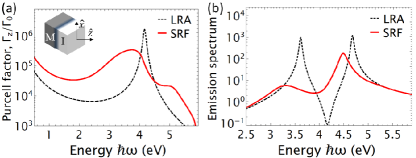
Figure 1: A QE with $z$-oriented transition dipole moment, placed $1\,$nm away from an air/Na IM interface. (a) Purcell factor and (b) emission spectrum (arbitrary units) within LRA (black dashed lines) and SRF (red solid lines).

The emission spectrum of a QE with transition energy $\hbar\omega_{0}=4.125\,$eV and free-space lifetime $\tau_{0}=0.1$ ns is presented in Fig. 1(b), where the Purcell factors of Fig. 1(a) are used. In the LRA description, the emission spectrum features two sharp peaks, splitting by $\hbar\Omega=1.06$ eV around the QE transition energy. When the quantum aspects of the response of the metal are introduced through SRF, the two emission peaks become broader, due to the higher material losses, but the Rabi splitting increases to $\hbar\Omega=1.3$ eV; the latter phenomenon stems from the dependence of the QE emission on the entire spectrum of the Purcell factor, which is higher within SRF away from the SPP resonance [Fig. 1(a)] christensen_prl118 .

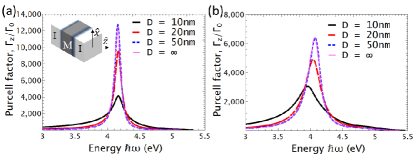
Figure 2: Purcell factor within (a) LRA and (b) SRF of a QE placed $5$ nm away from an IMI nanostructure, for different metal thicknesses $D=10$ (black solid line), 20 (red dotted line) and $50$ nm (blue dashed line). The thin purple shows the corresponding IM result.

Turning to the IMI case, where air is considered as the insulating medium, we examine the corresponding Purcell factor in Figs. 2(a) and (b) within LRA and SRF, respectively, for metal layer thicknesses $D=10,\,20$, and $50\,$nm. Specifically, we set the distance between the QE and the insulator/metal interface to $z_{\text{QE}}=5$ nm, noting that the Purcell factors calculated for the IM and the IMI geometry exhibit negligible differences for smaller values $z_{\text{QE}}\sim 2\,$ nm. In the case of LRA, the Purcell factor has its highest value at the SPP energy for all layer thicknesses. On the other hand, when SRF is taken into account, the maximum Purcell factor is roughly halved, and its peak positions redshift significantly as the metal thickness decreases. For the thinnest layer ($D=10\,$nm), the resonance within SRF has shifted by more than $\hbar\omega=0.2\,$eV compared to LRA. For increasing metal thickness (above $D=50\,$nm), the Purcell factor for the IMI case converges to the IM result.

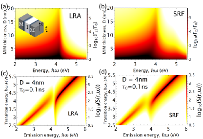
Figure 3: Contour plot of the Purcell factor of a QE, as a function of emission energy and dielectric layer thickness $D$, calculated within (a) LRA and (b) SRF, and the corresponding contours of the emission spectra (arbitrary units) as a function of the QE emission and transition energies obtained with (c) LRA and (d) SRF. The QE, with $\tau_{0}=0.1\,$ns, is placed in the middle of the insulator layer of an MIM structure with dielectric-layer thickness $D=4\,$nm.

While the IMI architecture can be instructive, in the remainder of the paper we will focus on the MIM structure, which is expected to display many of the advantages of plasmonic cavities discussed in the introduction —apart, perhaps, from the antenna effect that characterizes nanoparticle-on-mirror cavities baumberg_natmat2019 , which contain the QE within them and, when relatively large nanoparticles are involved, one can approximately assume that the QE experiences (locally) the cavity as a MIM. The investigation of QE relaxation inside MIM structures is thus an important first (exactly solvable) step towards understanding timely experimental works.

In Figs. 3(a,b) we compare LRA and SRF contour plots of the Purcell factor as a function of the QE emission energy and the thickness $D$ of the insulator layer (assumed air here) for a QE placed in the middle of the insulating gap ($z_{\text{QE}}=0$). In both plots, we observe that, for small $D$, the Purcell factor is significantly enhanced compared to the reference free-space value. In LRA, the peak of the Purcell factor coincides with the SPP resonance, while for higher energies there is a sharp drop of its value, related to the absence of plasmon polariton modes in the bandgap region of the MIM structure marocico_pra84 . On the other hand, SRF reproduces the expected redshift of the Purcell factor spectrum, while considerable enhancement is observed inside the bandgap, as a result of the quantum effects captured by the Feibelman parameters. As the thickness of the insulator increases, surface effects become less important and the spectra obtained within the two models converge. What is evident from the large Purcell-factor enhancements of Figs. 3(a,b) is that the QE–MIM interaction can enter the strong coupling regime, as verified by the emission-spectrum contour plots of Figs. 3(c,d), where clear anticrossings can be observed not only within LRA, but also in the SRF case. Naturally, the emission double-peak features are sharper in the LRA description, and are broadened when additional loss channels due to surface effects are considered, but the observed Rabi splitting clearly survives.

Having established the strong coupling regime, we turn now to the main focus of this paper, which is the QE dynamics. The QE excited-state population dynamics presented in Fig. 4 exhibits strong oscillations, with very different features from simple exponential relaxation within the Markovian (weak coupling) approximation, where memory effects in Eq. (4) are ignored. For a QE with transition energy $\hbar\omega_{0}=3\,$eV and vacuum relaxation rate $\tau_{0}=0.5\,$ns, Fig. 4(a) shows the excited state dynamics when $z_{\text{QE}}=1\,$nm in the IM geometry. In the LRA description, we observe that the relaxation follows an exponential pattern modified by rapid oscillations, where after a few of them the QE relaxes to the ground state within a time-span of $60\,$fs. Faster relaxation to the ground state is predicted in SRF, although a closer look in the inset of Fig. 4(a) reveals that in this case the excited state remains partially populated, $\left|c_{\text{nL}}\right|^{2}=0.003$, even at longer times, although is expected to fully relax due to interaction with the environment.

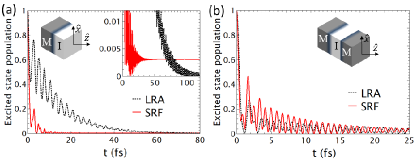
Figure 4: Population of the excited state of a two-level QE with $\hbar\omega_{0}=3\,$eV and $\tau_{0}=0.5\,$ns, as a function of time $t$. (a) The QE is placed $1\,$nm away from an IM geometry. (b) The QE is placed in the middle of a MIM geometry with dielectric-layer thickness $D=2\,$nm. In both panels, black and red lines correspond to results within LRA and SRF, respectively.

To directly compare the IM and MIM geometries, we consider a QE centered in an insulating (air) layer of $D=2\,$nm thickness sandwiched between metal regions, i.e., maintaining a $1\,$nm distance from the metal/dielectric interfaces. Here, the QE population dynamics presented in Fig. 4(b) is characterized by strong oscillatory behavior, with larger population values persisting over longer time spans. While in LRA calculations the QE eventually relaxes to the ground state within the considered time scale, the SRF calculations accounting for the quantum response predict that $\sim 3$% of the initial population remains in the excited state on the same time scale, a $10$-fold increase compared to the IM structure. The time scale of the plot is short compared to the QE lifetime, and complete relaxation will ultimately be achieved.

In Fig. 5 we present the excited-state population dynamics of a QE placed in the middle of a MIM cavity having an insulator (air) layer thickness of $D=2\,$nm when different free-space relaxation rates $\tau_{0}$ are considered. Choosing the associated QE transition energy matching the highest value shown in the Purcell factor spectra of Fig. 3, LRA and SRF models are contrasted in Figs. 5(a,b) for $\hbar\omega_{0}=4.13\,$eV and $\hbar\omega_{0}=3.43\,$eV, respectively. In both panels we observe strong and rapid Rabi oscillations; as the value of the free-space lifetime decreases from $\tau_{0}=10$ to $0.1\,$ns, the QE/MIM coupling increases, the oscillation period decreases, and non-Markovian effects become stronger, as anticipated. We also observe that the population oscillations are denser in the SRF case; the reason is that what is considered is the full Purcell-factor spectrum which, compared to the LRA case is broader, and the contribution to the bandgap region is also substantial, thus leading to a higher QE/MIM cavity interaction. The different values of $\tau$ are connected with the different possible natural or artificial QEs available for experimental manipulationBricks2018 ; Koperski2020 ; Epstein2020 .

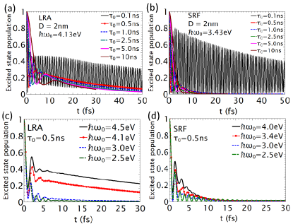
Figure 5: Population of the excited state of a two-level QE as a function of time, within LRA (a,c) and SRF (b,d). The QE is placed in the middle of a MIM geometry of thickness $D=2\,$nm. (a,b) The values of $\tau_{0}$ considered are displayed in the insets. The transition energy of the QE is $\hbar\omega_{0}=4.13\,$eV (LRA) and $\hbar\omega_{0}=3.43\,$eV (SRF). (c,d) The values of $\hbar\omega_{0}$ considered are shown in the insets, for a QE with $\tau_{0}=0.5\,$ns.

Finally, in Figs. 5(c,d) we explore the influence of the QE transition energy, $\hbar\omega_{0}$, on the population dynamics, taking a QE free-space lifetime of $\tau_{0}=0.5\,$ns. Different values of the QE transition energy are considered, including those matching the SPP energies indicated in the Purcell factor spectrum of Fig. 3. Fig. 5(c) shows the LRA calculation, where we observe that, after a few oscillations, the population dynamics remains partially trapped—although, eventually, it fully relaxes at later times. As the QE transition energy decreases, moving away from the SPP resonance energy associated with the highest Purcell factor enhancement, the partially transient trapped population steadily decreases. In the SRF case, we also observe a highly oscillatory behavior of the excited state population density, a sign that the non-Markovian signature is retained. Although the partially excited population trapping is smaller, strong oscillations are still present, with reduced period, indicating that the overall QE–MIM interaction is higher when the quantum aspects of the metal response are taken into account.

Summary — We theoretically explored the emission properties of a QE placed in proximity to IM, IMI, and MIM geometries in the weak- and strong-coupling regimes. Focusing on Na as a plasmonic metal whose nanoscopic optical response is dominated by electron spill-out, we adopted the quantum-informed SRF approach, in which the Feibelman $d$ parameters for the centroid of induced charge incorporate first-principles calculations. Although quantum effects introduce additional losses in the metal, the QE/MIM cavity system is found to operate in the strong-coupling regime, manifested as a Rabi splitting in the emission spectrum and through Rabi oscillations in the relaxation dynamics of the QE excited state, with a highly non-Markovian character. SRF bridges, therefore, ab initio approaches with classical EM calculations in a simple and elegant way, suitable not only for classical but also for quantum-optical dynamic studies at the nanoscale.

- (1) E. Ozbay, Science 311, 189 (2006).
- (2) P. Törmä and W. L. Barnes, Reports on Progress in Physics 78, 013901 (2015).
- (3) M. Pelton, Nature Photonics 9, 427 (2015).
- (4) S. I. Bozhevolnyi and J. B. Khurgin, Nature Photonics 11, 398 (2017).
- (5) J. J. Baumberg, J. Aizpurua, M. H. Mikkelsen, and D. R. Smith, Nature Materials 18, 668-678 (2019).
- (6) L. Mandel and E. Wolf, Optical Coherence and Quantum Optics (Cambridge University Press, 1995).
- (7) M. O. Scully and M. S. Zubairy, Quantum Optics (Cambridge University Press, 1997).
- (8) A. V. Akimov, A. Mukherjee, C. L. Yu, D. E. Chang, A. S. Zibrov, P. R. Hemmer, H. Park, and M. D. Lukin, Nature 450, 402 (2007).
- (9) D. E. Chang, A. S. Sørensen, E. A. Demler, and M. D. Lukin, Nature Physics 3, 807 (2007).
- (10) A. Goban, C.-L. Hung, S.-P. Yu, J. Hood, J. Muniz, J. Lee, M. Martin, A. McClung, K. Choi, D. Chang, O. Painter, and H. Kimble, Nature Communications 5, 3808 (2014).
- (11) J. D. Hood, A. Goban, A. Asenjo-Garcia, M. Lu, S.-P. Yu, D. E. Chang, and H. J. Kimble, Proceedings of the National Academy of Sciences 113, 10507 (2016).
- (12) A. I. Fernández-Domínguez, S. I. Bozhevolnyi, and N. A. Mortensen, ACS Photonics 5, 3447 (2018).
- (13) M. Koperski, D. Vaclavkova, K. Watanabe, T. Taniguchi, K. S. Novoselov, and M. Potemski, Proceedings of the National Academy of Sciences 117, 13214 (2020).
- (14) C. Manolatou and F. Rana, IEEE Journal of Quantum Electronics 44, 435 (2008).
- (15) G. M. Akselrod, C. Argyropoulos, T. B. Hoang, C. Ciracì, C. Fang, J. Huang, D. R. Smith, and M. H. Mikkelsen, Nature Photonics 8, 835 (2014).
- (16) A. Rose, T. B. Hoang, F. McGuire, J. J. Mock, C. Ciracì, D. R. Smith, and M. H. Mikkelsen, Nano Letters 14, 4797 (2014).
- (17) R. Chikkaraddy, B. de Nijs, F. Benz, S. J. Barrow, O. A. Scherman, E. Rosta, A. Demetriadou, P. Fox, O. Hess, and J. J. Baumberg, Nature 535,127 (2016).
- (18) M. A. May, D. Fialkow, T. Wu, K.-D. Park, H. Leng, J. A. Kropp, T. Gougousi, P. Lalanne, M. Pelton, and M. B. Raschke, Advanced Quad. Tech. 3, 1900087 (2020).
- (19) S. I. Bogdanov, M. Y. Shalaginov, A. S. Lagutchev, C.-C. Chiang, D. Shah, A. S. Baburin, I. A. Ryzhikov, I. A. Rodionov, A. V. Kildishev, A. Boltasseva, and V. M. Shalaev, Nano Letters 18, 4837 (2018).
- (20) J. M. Katzen, C. Tserkezis, Q. Cai, L. H. Li, J. M. Kim, G. Lee, G.-R. Yi, W. R. Hendren, E. J. G. Santos, R. M. Bowman, and F. Huang, ACS Applied Materials & Interfaces 12, 19866 (2020).
- (21) O. S. Ojambati, W. M. Deacon, R. Chikkaraddy, C. Readman, Q. Lin, Z. Koczor-Benda, E. Rosta, O. A. Scherman, and J. J. Baumberg, ACS Photonics 7, 2337 (2020).
- (22) F. Ding, Y. Yang, R. A. Deshpande, and S. I. Bozhevolnyi, Nanophotonics 7, 1129 (2018).
- (23) U. Hohenester, Nano and Quantum Optics: An Introduction to Basic Principles and Theory (Springer, 2020).
- (24) C. Ciracì, R. T. Hill, J. J. Mock, Y. Urzhumov, A. I. Fernández-Domínguez, S. A. Maier, J. B. Pendry, A. Chilkoti, and D. R. Smith, Science 337, 1072 (2012).
- (25) K. J. Savage, M. M. Hawkeye, R. Esteban, A. G. Borisov, J. Aizpurua, and J. J. Baumberg, Nature 491, 574 (2012).
- (26) J. A. Scholl, A. L. Koh, and J. A. Dionne, Nature 483, 421 (2012).
- (27) I. Romero, J. Aizpurua, G. W. Bryant, F. J. García de Abajo, Optics Express 14, 9988 (2006).
- (28) R. Esteban, A. G. Borisov, P. Nordlander and J. Aizpurua, Nature Communications 3, 825 (2012).
- (29) Y. Luo, A. I. Fernández-Domínguez, A. Wiener, S. A. Maier and J. B. Pendry, Physical Review Letters 111, 093901 (2013).
- (30) S. Raza, N. Stenger, S. Kadkhodazadeh, S. V. Fischer, N .Kostesha, A.-P. Jauho, A. Burrows, M. Wubs, and N. A. Mortensen, Nanophotonics 2, 131 (2013).
- (31) Y. Yang, D. Zhu, W. Yan, A. Agarwal, M. Zheng, J. D. Joannopoulos, P. Lalanne, T. Christensen, K. K. Berggren, and M. Soljačić, Nature 576, 248 (2019).
- (32) A. Moreau, C. Ciracì, and D. R. Smith, Physical Review B 87, 045401 (2013).
- (33) S. Raza, T. Christensen, M. Wubs, S. I. Bozhevolnyi, and N. A. Mortensen, Physical Review B 88, 115401 (2013).
- (34) N. A. Mortensen, S. Raza, M. Wubs, T. Søndergaard, and S. I. Bozhevolnyi, Nature Communications 5, 3809 (2014).
- (35) C. Tserkezis, A. T. M. Yeşilyurt, J.-S. Huang, and N. A. Mortensen, ACS Photonics 5, 5017 (2018).
- (36) G. Toscano, J. Straubel, A. Kwiatkowski, C. Rockstuhl, F. Evers, H. Xu, N. A. Mortensen and M. Wubs, Nature Communications 6, 7132 (2015).
- (37) W. Yan, Physical Review B 91, 115416 (2015).
- (38) C. Ciracì and F. Della Sala, Physical Review B 93, 205405 (2016).
- (39) C. Ciracì, R. Jurga, M. Khalid, and F. Della Sala, Nanophotonics 8, 1821 (2019).
- (40) A. Varas, P. García-González, J. Feist, F. García-Vidal, and A. Rubio, Nanophotonics 5, 409 (2016).
- (41) P. Feibelman, Progress in Surface Science 12, 287 (1982).
- (42) W. Yan, M. Wubs, and N. Asger Mortensen, Physical Review Letters 115, 137403 (2015).
- (43) T. Christensen, W. Yan, A.-P. Jauho, M. Soljačić, and N. A. Mortensen, Physical Review Letters 118, 157402 (2017).
- (44) P. A. D. Gonçalves, T. Christensen, N. Rivera, A.-P. Jauho, N. A. Mortensen, and M. Soljačić, Nature Communications 11, 366 (2020).
- (45) N. A. Mortensen, Nanophotonics 10, 2563 (2021).
- (46) N. Rivera and I. Kaminer, Nature Reviews Physics 2, 538 (2020).
- (47) K. Head-Marsden, J. Flick, C. J. Ciccarino, and P. Narang, Chemical Reviews 121 (2021), 10.1021/acs.chemrev.0c00620.
- (48) P. Lalanne, W. Yan, K. Vynck, C. Sauvan, and J.-P. Hugonin, Laser & Photonics Reviews 12, 1700113 (2018).
- (49) M. K. Dezfouli, C. Tserkezis, N. A. Mortensen, and S. Hughes, Optica 4, 1503 (2017).
- (50) S. Franke, S. Hughes, M. K. Dezfouli, P. T. Kristensen, K. Busch, A. Knorr, and M. Richter, Physical Review Letters 122, 213901 (2019).
- (51) C.-J. Yang and J.-H. An, Phys. Rev. B 95, 161408(R) (2017).
- (52) I. Thanopulos, V. Karanikolas, N. Iliopoulos, and E. Paspalakis, Physical Review B 99, 195412 (2019).
- (53) C.-J. Yang, J.-H. An, and H.-Q. Lin, Phys. Rev. Research 1, 023027, (2019).
- (54) C. Tserkezis, N. Stefanou, M. Wubs, and N. A. Mortensen, Nanoscale 8, 17532 (2016).
- (55) T. Christensen, W. Yan, S. Raza, A.-P. Jauho, N. A. Mortensen, and M. Wubs, ACS Nano 8, 1745 (2014).
- (56) C. Tserkezis, M. Wubs, and N. A. Mortensen, ACS Photonics 5, 133 (2018).
- (57) C. Tserkezis, A. I. Fernández-Domínguez, P. A. D. Gonçalves, F. Todisco, J. D. Cox, K. Busch, N. Stenger, S. I. Bozhevolnyi, N. A. Mortensen, and C. Wolff, Reports on Progress in Physics 83, 082401 (2020).
- (58) C. L. C. Smith, N. Stenger, A. Kristensen, N. A. Mortensen, and S. I. Bozhevolnyi, Nanoscale 7, 9355 (2015).
- (59) H. T. Dung, L. Knöll, and D.-G. Welsch, Physical Review A 65, 043813 (2002).
- (60) C. T. Tai, Dyadic Green Functions in Electromagnetic Theory (Oxford University Press, Oxford, 1994).
- (61) S. Scheel and S. Y. Buhmann, Acta Physical Slovaca 58 675 (2009).
- (62) A. F. Koenderink, Opt. Lett. 35, 4208 (2010).
- (63) F. J. García de Abajo, Journal of Physical Chemistry C 112, 17983 (2008).
- (64) A. Rodríguez Echarri, P. A. D. Gonçalves, C. Tserkezis, F. J. García de Abajo, N. A. Mortensen, and J. D. Cox, Optica 8, 710 (2021).
- (65) See Supplemental Material for details on the calculation of the Green’s tensor for the IM, IMI and MIM geometries including the SRF boundury conditions. The macroscopic QED theory is used to extract Eqs. (3) and (4).
- (66) C. Van Vlack, P. T. Kristensen, and S. Hughes, Physical Review B 85, 075303 (2012).
- (67) V. Karanikolas, I. Thanopulos, and E. Paspalakis, Physical Review Research 2, 033141 (2020).
- (68) A. Gonzalez-Tudela, P. A. Huidobro, L. Martín-Moreno, C. Tejedor, and F. J. García-Vidal, Physical Review B 89, 041402(R) (2014).
- (69) R.-Q. Li, D. Hernángomez-Peréz, F. J. García-Vidal, and A. I. Fernández-Domínguez, Physical Review Letters 117, 107401 (2016).
- (70) I. Thanopulos, V. Yannopapas, and E. Paspalakis, Physical Review B 95, 075412 (2017).
- (71) A. Delga, J. Feist, J. Bravo-Abad, and F. J. Garcia-Vidal, Physical Review Letters 112, 253601 (2014).
- (72) C. Tserkezis, N. A. Mortensen, and M. Wubs, Physical Review B 96, 085413 (2017).
- (73) A. J. Bennett, Phys. Rev. B 1, 203 (1970).
- (74) M. K. Svendsen, C. Wolff, A.-P. Jauho, N. A. Mortensen, and C. Tserkezis, J. Phys.: Condens. Matter 32, 395702 (2020).
- (75) C. A. Marocico and J. Knoester, Physical Review A 84, 053824 (2011).
- (76) J.L. Bricks, Y.L. Slominskii, I.D. Panas, and A.P. Demchenko, Methods Appl. Fluoresc. 6, 012001 (2018).
- (77) M. Koperski, D. Vaclavkova, K. Watanabe, T. Taniguchi, K.S. Novoselov, and M. Potemski, PNAS 117, 13214 (2020).
- (78) I. Epstein, A.J. Chaves, D.A. Rhodes, B. Frank, K. Watanabe, T. Taniguchi, H. Giessen, J.C. Hone, N.M.R. Peres, and F.H.L. Koppens, 2D Materials 7, 035031 (2020).