Enhancing gravitational-wave burst detection confidence in expanded detector networks with the BayesWave pipeline

Abstract

The global gravitational-wave detector network achieves higher detection rates, better parameter estimates, and more accurate sky localisation, as the number of detectors, $\mathcal{I}$ increases. This paper quantifies network performance as a function of $\mathcal{I}$ for BayesWave, a source-agnostic, wavelet-based, Bayesian algorithm which distinguishes between true astrophysical signals and instrumental glitches. Detection confidence is quantified using the signal-to-glitch Bayes factor, $\mathcal{B}_{\mathcal{S},\mathcal{G}}$. An analytic scaling is derived for $\mathcal{B}_{\mathcal{S},\mathcal{G}}$ versus $\mathcal{I}$, the number of wavelets, and the network signal-to-noise ratio, SNR${}_{\text{net}}$, which is confirmed empirically via injections into detector noise of the Hanford-Livingston (HL), Hanford-Livingston-Virgo (HLV), and Hanford-Livingston-KAGRA-Virgo (HLKV) networks at projected sensitivities for the fourth observing run (O4). The empirical and analytic scalings are consistent; $\mathcal{B}_{\mathcal{S},\mathcal{G}}$ increases with $\mathcal{I}$. The accuracy of waveform reconstruction is quantified using the overlap between injected and recovered waveform, $\mathcal{O}_{\text{net}}$. The HLV and HLKV network recovers $87\%$ and $86\%$ of the injected waveforms with $\mathcal{O}_{\text{net}}>0.8$ respectively, compared to $81\%$ with the HL network. The accuracy of BayesWave sky localisation is $\approx 10$ times better for the HLV network than the HL network, as measured by the search area, $\mathcal{A}$, and the sky areas contained within $50\%$ and $90\%$ confidence intervals. Marginal improvement in sky localisation is also observed with the addition of KAGRA.

I Introduction

The Laser Interferometer Gravitational-Wave Observatory (LIGO) LIGO2015 ; 2009RPPh…72g6901A ; Harry_2010 has completed three observing runs, O1 2017PhRvD..95d2003A ; 2019PhRvX…9c1040A , O2 2019PhRvD.100b4017A ; 2019PhRvX…9c1040A and O3 2020NatRP…2..222G between 2015 to 2020, including joint searches with Italian partner, Virgo 2015CQGra..32b4001A , in the final month of O2 and the whole of O3. In April 2019, Advanced LIGO commenced its third observing run in collaboration with Advanced Virgo as a three-detector network: the Hanford-Livingston-Virgo (HLV) network. The Kamioka Gravitational Wave Detector (KAGRA) 2019CQGra..36p5008A ; 2020arXiv200505574A ; 2013PhRvD..88d3007A also began observing in February 2020 2020NatRP…2..222G .

With access to these upgraded instruments, there is a burgeoning interest in detecting short-duration gravitational wave (GW) signals by combining data from multi-detector networks. These signals typically have durations of milliseconds up to a few seconds, with the most common sources being compact binary coalescences (CBCs) such as black hole or neutron star mergers, along with other potential sources like core-collapse supernovae (SNe) of massive stars 2011LRR….14….1F , pulsar glitches of astrophysical origin 2014ApJ…787..114S and cusps in cosmic strings 2005PhRvD..71f3510D . In addition to these known sources, it is also plausible to detect transient signals of unknown astrophysical origin.

Searches for generic GW transients, or burst searches, require the ability to distinguish such signals from any noise artefacts present in the detector data. Hence, it is crucial to understand the noise properties of the detector data. Results from the initial LIGO-Virgo science runs revealed non-stationary and non-Gaussian detector noise, which includes short-duration noise transients denoted by the term ‘glitches’ 2008CQGra..25r4004B ; 2015CQGra..32k5012A ; 2012CQGra..29o5002A . If not accounted for properly, these features could resemble GWs and consequently limit the ability to detect low-amplitude signals.

Since CBC signals come from known and well-studied sources, such signals are accurately modelled in most regions of parameter space and therefore can be detected with high confidence using matched-filter searches 2016CQGra..33u5004U ; 2019arXiv190108580S ; 2012PhRvD..86b4012H . Other GW bursts signals, on the other hand, may originate from either complex or unanticipated sources. Given the stochastic nature and complexity of the potential sources (e.g. core collapse supernovae), there are no robust models available to date to assist with the searches of generic burst signals, making it challenging to distinguish them from other non-Gaussian features like glitches in the detector data, as well as to accurately reconstruct the underlying signal waveform.

There are a number of unmodelled burst searches performed in LIGO and Virgo data 2017PhRvD..95j4046L ; cWB . In this work we look at an unmodelled search algorithm called BayesWave 2015PhRvD..91h4034L ; 2015CQGra..32m5012C ; BWIII , which was proposed to enable the joint detection and characterisation of GW bursts and instrumental glitches. BayesWave reconstructs both signals and glitches as a sum of sine-Gaussian wavelets, where the number of wavelets and their parameters are determined via a reversible-jump Markov chain Monte Carlo (RJMCMC) algorithm. Bayesian model selection is then used to determine the likelihood of an event being a true signal, or a noise artefact.

Previous studies have quantified the performance of BayesWave in recovering simulated waveforms from simulated noise with a two-detector network (HL network) 2016PhRvD..94d4050L ; 2016PhRvD..93b2002K . However, with Virgo joining GW searches alongside the HL-network in O2 and O3, KAGRA coming online towards the end of O3, and future detectors like LIGO-India in the planning stages 2013IJMPD..2241010U , the network of GW detectors is expanding rapidly. Expanding detector networks will increase the likelihood of detecting more events with higher confidence. These improvements are evident in previous studies and will be elaborated further in Section II.

In this paper, we aim to evaluate BayesWave’s performance in searching for GW bursts from detector data beyond the HL-network. We achieve this by using BayesWave to recover injected signals from simulated noise with the HLV and the HLKV detector networks, and comparing the outcomes with those of the HL network. We quantify the performance of BayesWave based on the following metric: (i) Bayes factor between signal and glitch models, (ii) overlap (match) between injected and recovered waveforms, and (iii) accuracy of recovered sky location. In Section III, we provide a detailed overview of the BayesWave algorithm. We derive the analytic scaling relation of the signal-to-glitch Bayes factor in Section IV. We then discuss the methods of injecting simulated waveforms into simulated detector noise samples in Section V, followed by comparisons and analyses of the metrics mentioned above: Bayes Factor in Section A, overlap in Section B and sky localisation in Section C. Finally, we present a summary of the results along with their implications in Section VII.

II Benefits of Expanding Detector Networks

Increasing the number of operational ground-based detectors has several major benefits for GW astronomy, including a higher rate of detection of GW transients, and better characterisation of those signals. Here we discuss some of the benefits of adding new detectors to the existing network.

A SNR and search volume

One major advantage of a larger detector network is the ability to confidently detect quieter events. The strain amplitude, $s^{(i)}$ in detector $i$ of the network consists of a signal, $h^{(i)}$ (if present) and detector noise, $n^{(i)}$ which can be expressed as

$$s^{(i)}=h^{(i)}+n^{(i)}.$$ (1)

The squared matched-filter signal-to-noise ratio (SNR) of signal $h^{(i)}_{s}$ in detector $i$ is then given by 1994PhRvD..49.2658C

$$\text{SNR}_{i}^{2}=\left(h^{(i)}_{s}\,\middle|\,h^{(i)}_{s}\right)$$ (2)

where $(.|.)$ on the right-hand-side of the expression is the noise-weighted inner product. We define the noise-weighted inner product between two arbitrary waveforms $h_{a}(t)$ and $h_{b}(t)$ as keppel…2009

$$\left(h_{a}\,\middle|\,h_{b}\right)=\int_{0}^{\infty}\frac{\tilde{h_{a}}^{*}(f)\tilde{h_{b}}(f)+\tilde{h_{a}}(f)\tilde{h_{b}}^{*}(f)}{S_{n}(f)}\,df.$$ (3)

where $\tilde{h}(f)$ is the Fourier-transformed waveform, $\tilde{h}^{*}(f)$ is its complex conjugate and $S_{n}(f)$ is the one-sided power spectral density (PSD) of stationary, Gaussian detector noise.

For a network with $\mathcal{I}$ detectors, the overall network SNR is given by 2016PhRvD..94d4050L

$$\text{SNR}_{\text{net}}^{2}=\sum_{i=1}^{\mathcal{I}}\text{SNR}_{i}^{2}$$ (4)

According to Equation 4, adding more detectors to the network increases the SNR of all detected GW signals. This enables detection pipelines to estimate waveform parameters more accurately 2017CQGra..34q4003G . With improved parameter estimates, more accurate models can be constructed to represent the detected waveform 2017ApJ…839…15B .

In addition, the SNR of GW signals scales with luminosity distance, $D_{L}$ as 2014arXiv1409.0522C

$$\text{SNR}_{i}\propto\frac{1}{D_{L}}.$$ (5)

By combining Equations 4 and 5 and assuming coherent searches, the overall SNR for a network of $\mathcal{I}$ detectors with equal sensitivities is given by $\text{SNR}_{\text{net}}\propto\sqrt{\mathcal{I}}/D_{L}$. Assuming that GW sources are uniformly distributed across the sky, an $\mathcal{I}$-detector network can detect $\sqrt{\mathcal{I}}$ times further and up to $\sqrt{\mathcal{I}^{3}}$ more sources compared to a single detector network since the search volume scales as $V\propto D_{L}^{3}$.

B Sky coverage

The sensitivity of a detector towards a particular sky location is determined by the antenna pattern in that given direction. Adding more detectors to the network at different geographical locations and orientations increases the sensitivity of the network to a wider region of the sky (increased sky coverage), consequently increasing the detection rate and volume along those directions 2011CQGra..28l5023S .

Reference 2012arXiv1202.4031M presented a visual comparison between the network antenna pattern across the whole sky between a three-detector (HLV) network and a four-detector (HLKV) network, where ‘K’ denotes KAGRA. As expected, results show that both networks are more sensitive to some regions in the sky than others. However, the HLKV network has higher overall network antenna power pattern and an overall increase in sky coverage is also reflected in the expansion of regions with relatively higher sensitivity.

C Observing time

Adding detectors to the existing network also increases the duty cycle where two or more detectors are functional and simultaneously observing. This consequently increases the chances of the detectors picking up a coherent astrophysical signal and leading to higher detection rates 2011CQGra..28l5023S .

D Sky localisation

Sky localisation of a GW source is of vital importance for locating and identifying any existing electromagnetic counterparts to the GW event 2018ApJ…854L..25P . Ground-based GW detectors are nearly omnidirectional, so with a single detector we are not able to impose a strict constrains to the sky location of a GW event. Nevertheless, sky localisation of GW signals improves significantly with multiple interferometers. The times of arrival at two detectors constrain the position of the source to an error ellipse in the sky map. Thus, having more detectors will reduce localisation volume by imposing stricter constraints to the location of the sources, improving the accuracy of locating the source in the sky 2018MNRAS.479..601D ; 2018ApJ…854L..25P . .

To sum up the points above, the advantages of having more detectors in the network include: (i) improvement in SNR and increased search volume, (ii) alignment-dependent sky coverage, (iii) increased rates of detection, and (iv) improved sky localisation.

III BayesWave Overview

BayesWave is a Bayesian data analysis algorithm that detects transient features in a stretch of detector data and identifies whether they are an astrophysical signal or instrumental noise. BayesWave reconstructs non-Gaussian features in the data using a sum of sine-Gaussian (also called Morlet-Gabor) wavelets. The number of wavelets and their respective parameters are sampled using a trans-dimensional Markov Chain Monte Carlo algorithm, otherwise known as the Reversible-Jump Markov Chain Monte Carlo (RJMCMC). The RJMCMC is implemented to allow for adjustable number of wavelets and hence variable model dimensions. BayesWave outputs posterior distributions and Bayesian evidences for three separate models: (i) Gaussian noise only, (ii) Gaussian noise with glitches and (iii) Gaussian noise with GW signal. The model evidences are then used for Bayesian model selection between the three scenarios.

A Wavelet Frames

BayesWave uses a sum of sine-Gaussian (also called Morlet-Gabor) wavelets to reconstruct non-Gaussian features (either signals or glitches) in the detector data. Even though Sine-Gaussian wavelets form a non-orthogonal frames, their shape is variable in time-frequency plane and can optimally reconstruct a transient GW signal with no a priori assumption on the signal source or morphology.

The number of wavelets used in the reconstruction is marginalised via the RJMCMC, where signals with complex structure in time-frequency plane will use more wavelets in the reconstruction. Previous studies 2016PhRvD..94d4050L ; 2018PhRvD..97j4057M have shown that the number of wavelets scales linearly with SNR such that

$$N\approx\gamma+\beta\text{ SNR}$$ (6)

where $\gamma$ and $\beta$ are constants which depend on waveform morphology. The results from Ref. 2016PhRvD..94d4050L show that $\beta$ and hence $N$ increase with waveform complexity. For binary black hole (BBH) waveforms, the typical numbers are $\gamma=5.6$ and $\beta=0.066$ for sine-Gaussian wavelet reconstructions 2018PhRvD..97j4057M .

In BayesWave, each wavelet in the time domain has five intrinsic parameters $t_{0},f_{0},Q,A,\phi_{0}$ which represent central time, central frequency, quality factor, amplitude and phase offset respectively. These intrinsic parameters can be expressed as a single parameter vector ${\bf\it\lambda}=\{t_{0},f_{0},Q,A,\phi_{0}\}$ and the mathematical representation of a sine-Gaussian wavelet is given by

$$\Psi(t;t_{0},f_{0},Q,A,\phi_{0})=Ae^{-\Delta t^{2}/\tau^{2}}\cos(2\pi f_{0}\Delta t+\phi_{0})$$ (7)

with $\tau=Q/(2\pi f_{0})$ and $\Delta t=t-t_{0}$ 2016PhRvD..94d4050L .

The glitch model in BayesWave is independent between detectors owing to the fact that noise artefacts are uncorrelated across different detectors. Hence, the set of glitch model parameters must contain the respective parameters for each individual detector across the network. The complete set of glitch model parameters for a network of detectors comprising Hanford, Livingston, and Virgo (HLV) can be written as 2016PhRvD..94d4050L

$${\bf\it\theta_{\mathcal{G}}}=\{{\bf\it\lambda}^{H}\cup{\bf\it\lambda}^{L}\cup{\bf\it\lambda}^{V}\}$$ (8)

with ${\bf\it\lambda}^{i}=\{{\bf\it\lambda}_{0}^{i}\cup{\bf\it\lambda}_{1}^{i}\cup\cdots\cup{\bf\it\lambda}_{N^{\mathcal{G}}_{i}}^{i}\}$ where the numerical subscripts indicate a single wavelet used in the glitch model and $N^{\mathcal{G}}$ is the total number of wavelets in the glitch model. The superscripts indicates the $i$-th detector in the network.

In contrast to the glitch model, the signal model is common across all detectors in the network. As a result, signal models should have a single set of intrinsic wavelet parameters ${\bf\it\lambda}^{\oplus}=\{{\bf\it\lambda}_{0}\cup{\bf\it\lambda}_{1}\cup\cdots\cup{\bf\it\lambda}_{N^{\mathcal{S}}}\}$, along with a set of extrinsic parameter ${\bf\it\Omega}=\{\alpha,\delta,\psi,\epsilon\}$ which sequentially describes the right ascension (RA), declination (dec), polarisation angle and ellipticity of the GW signal. The sky location (RA, dec) and polarisation angle of a source determine antenna beam patterns of the detector network, as well as provide information on the amplitude and the arrival-time delay of the signal in each detector 2004ARNPS..54..525C . Ellipticity defines the relative phase and amplitude of the plus and cross polarisations, $h_{+}$ and $h_{\times}$ respectively with $h_{\times}=\epsilon h_{+}e^{i\pi/2}$. The ellipticity parameter, $\epsilon$ takes values between $0$ to $1$ with the lower and upper bounds denoting linear to circular polarisations respectively 2015CQGra..32m5012C . Altogether a complete set of signal model parameters is given by 2016PhRvD..94d4050L

$${\bf\it\theta_{\mathcal{S}}}=\{{\bf\it\lambda}^{\oplus}\cup{\bf\it\Omega}\}.$$ (9)

BayesWave produces posterior distributions of the parameters described above. Each draw from the posterior contains a unique set of wavelet parameters (and extrinsic parameters for the signal model), which are then summed to produce a posterior on the waveform, $h(t)$. By using this basis of sine-Gaussian wavelets, $h(t)$ is reconstructed with no a priori assumption on the source of the GW signal.

B Model Selection

In addition to waveform reconstruction, BayesWave performs model selection between the signal and glitch hypotheses described above. The ratio of model evidences, otherwise known as the Bayes factor, is the key to model selection in Bayesian inference as it assesses the plausibility of two different models, $\mathcal{M}_{\alpha}$ and $\mathcal{M}_{\beta}$, parameterised by their respective parameter sets $\vec{\theta}_{\alpha}$ and $\vec{\theta}_{\beta}$. In other words, it quantifies which model is better supported by the data. The model evidence (also called the margainalised evidence) is given by

$$p(\vec{s}|\mathcal{M}_{\alpha})=\int p(\vec{\theta}_{\alpha}|\mathcal{M}_{\alpha})p(\vec{s}|\vec{\theta}_{\alpha},\mathcal{M}_{\alpha})d\vec{\theta}_{\alpha}$$ (10)

where $\vec{s}$ is the observed data, $\mathcal{M}_{\alpha}$ is the model, and $\vec{\theta}_{\alpha}$ is there parameter vector for model $\mathcal{M}_{\alpha}$. The prior probability of parameters $\vec{\theta}_{\alpha}$ before the data are observed is given by $p(\vec{\theta}_{\alpha}|\mathcal{M}_{\alpha})$, and $p(\vec{s}|\vec{\theta}_{\alpha},\mathcal{M}_{\alpha})$ is the likelihood of obtaining the observed data $\vec{s}$, given the model $\mathcal{M}_{\alpha}$. Hence, the Bayes factor between models $\mathcal{M}_{\alpha}$ and $\mathcal{M}_{\beta}$, parameterised by their respective parameter vectors $\vec{\theta}_{\alpha}$ and $\vec{\theta}_{\beta}$ is

$$\begin{split}\mathcal{B}_{\alpha,\beta}(\vec{s})&=\frac{p(\vec{s}|\mathcal{M}_{\alpha})}{p(\vec{s}|\mathcal{M}_{\beta})}.\end{split}$$ (11)

$\mathcal{B}_{\alpha,\beta}(\vec{s})>1$ implies that model $\mathcal{M}_{\alpha}$ is more strongly supported by the data than model $\mathcal{M}_{\beta}$. To reduce computational costs, the BayesWave algorithm calculates model evidence using thermodynamic integration 2009PhRvD..80f3007L .

BayesWave calculates the Bayes factor between the signal model (i.e. the data contains a real astrophysical signal), and the glitch model (i.e. the data contains an instrumetnal glitch). In Section IV we discuss how the signal-to-glitch Bayes factor scales with SNR, the number of wavelets used in the MCMC, and the number of detectors in the network.

C Overlap

In addition to distinguishing between signals and glitches, BayesWave also produces a posterior distribution of the wavelet-expanded waveforms, $h(t)$ to match the true waveform, $h_{s}(t)$. One way to quantify the agreement or similarity between $h(t)$ and $h_{s}(t)$ is through the overlap, $\mathcal{O}$. Reconstructed waveforms in BayesWave are analogous to waveform templates, hence the overlap between reconstructed models and the injected waveform can be computed the same way as the overlap in matched-filtering.

The normalised overlap between the two waveforms can be written as 2017ApJ…839…15B

$$\mathcal{O}=\frac{\left(h\,\middle|\,h_{s}\right)}{\sqrt{\left(h\,\middle|\,h\right)\left(h_{s}\,\middle|\,h_{s}\right)}}$$ (12)

where $(.|.)$ is the noise-weighted inner product as defined in Equation 3. Since Equation 12 is normalised, $\mathcal{O}$ takes values between $-1$ to $1$. When $\mathcal{O}=1$, there is a perfect match between the injected and recovered waveform; $\mathcal{O}=0$ implies that there is no match at all and $\mathcal{O}=-1$ implies a perfect anti-correlation.

Equation 12 only applies to a single detector. A network overlap, $\mathcal{O_{\text{net}}}$ is required to fully evaluate BayesWave’s performance in recovering waveforms from all the detectors combined. In order to define the network overlap, we sum each factor in Equation 12 over all $\mathcal{I}$ detectors in the network such that

$$\mathcal{O_{\text{net}}}=\frac{\sum_{i=1}^{\mathcal{I}}\left(h^{(i)}\,\middle|\,h_{s}^{(i)}\right)}{\sqrt{\sum_{i=1}^{\mathcal{I}}\left(h^{(i)}\,\middle|\,h^{(i)}\right)\sum_{i=1}^{\mathcal{I}}\left(h_{s}^{(i)}\,\middle|\,h_{s}^{(i)}\right)}},$$ (13)

where $h^{(i)}$ and $h_{s}^{(i)}$ denote the recovered waveform and waveform present in detector $i$ respectively.

IV Analytic Bayes Factor Scaling

In this work, we aim to understand the behavior of the Bayes factor between signal and glitch models for networks comprising different numbers of GW detectors. Hence it is in our interest to analytically understand the conditions of model selection. We want to know under what circumstances a model is favoured over another.

A Occam Penalty

A key to understanding Bayes factor behavior when using a trans-dimensional model as BayesWave does, is the role of the Occam penalty.

The parameter value at which the posterior distribution peaks is known as the maximum a posteriori (MAP) value, denoted as $\vec{\theta}_{\text{MAP}}$. For high SNR events, the integrand of model evidence in Equation 10 peaks sharply in the vicinity of the MAP. Following the Laplace-Fisher approximation, the integral can be estimated as

$$p(\vec{s}|\mathcal{M})\simeq p(\vec{s}|\vec{\theta}_{\text{MAP}},\mathcal{M})p(\vec{\theta}_{\text{MAP}}|\mathcal{M})(2\pi)^{D/2}\sqrt{\text{det}C}.$$ (14)

where $p(\vec{s}|\vec{\theta}_{\text{MAP}},\mathcal{M})$ is the MAP likelihood; $p(\vec{\theta}_{\text{MAP}}|\mathcal{M})$ is the prior evaluated at the MAP parameter values; $D$ is the dimension of the model; and $\det C$ is the determinant of the full covariance matrix for the $N$ wavelets used in waveform reconstruction. If the covariance matrix for a single wavelet is $C_{n}$, then we have

$$\det C=\prod^{N}_{n=1}\det C_{n},$$ (15)

assuming minimal overlap between the wavelet parameter spaces. Since the Laplace-Fisher approximation is associated with the MAP likelihood, the covariance matrix can be approximated as the inverse of the Fisher Information Matrix (FIM), $\Gamma$ doi:10.2307/3315678 . A comprehensive discussion of the FIM and its relation to wavelet parameter jump proposal is presented in Appendix A.

By definition, $\det C$ measures the variance of the likelihood. Thus, $\sqrt{\det C}$ quantifies the characteristic spread of the likelihood function. The product of $\sqrt{\det C}$ and $(2\pi)^{D/2}$, which account for the dimensionality of the model, can then be used as a measure for the volume of the uncertainty ellipsoid (posterior volume), $\Delta V_{\mathcal{M}}$ for a given model $\mathcal{M}$ 2016PhRvD..94d4050L ; 2017LRR….20….2R ; littenberg…2009 . Assuming uniform priors for all wavelet parameters, one can also write $p(\vec{\theta}_{\text{MAP}}|\mathcal{M})=1/V_{\mathcal{M}}$ where $V_{\mathcal{M}}$ represents the total parameter space volume. Hence, the last three factors of Equation 14 can collectively be interpreted as the fraction of the prior occupied by the posterior distribution, such that the model evidence is now given by

$$p(\vec{s}|\mathcal{M})\simeq p(\vec{s}|\vec{\theta}_{\text{MAP}},\mathcal{M})\frac{\Delta V_{\mathcal{M}}}{{V_{\mathcal{M}}}}.$$ (16)

where $\Delta V_{\mathcal{M}}/V_{\mathcal{M}}$ is the “Occam penalty factor”.

Following equations 11 and 16, the Bayes factor between two models can be re-expressed as

$$\mathcal{B}_{\alpha,\beta}(\vec{s})=\Lambda_{\alpha,\beta}(\vec{s})\frac{\Delta V_{\alpha}}{V_{\alpha}}\frac{V_{\beta}}{\Delta V_{\beta}}$$ (17)

where the ratio of MAP likelihoods is given by

$$\Lambda_{\alpha,\beta}(\vec{s}) =\frac{p(\vec{s}|\vec{\theta}_{\text{MAP},\alpha})}{p(\vec{s}|\vec{\theta}_{\text{MAP},\beta})}.$$ (18)

Equation 17 suggests that the Bayes factor is dependent on the likelihood ratio and the ratio of the Occam penalty factors. The Occam factor penalises models that require an unnecessarily large parameter space volume to fit the data by suppressing the model evidence. Note that Occam penalty is not an intentionally added component to the Bayes factor, rather it is inherently imposed as a result of using the Bayes Theorem.

As a heuristic explanation as to how the Occam penalty aids in BayesWave’s ability to distinguish between signals and glitches, recall that signal models ($\mathcal{S}$) for each detector share the same intrinsic parameters and four extrinsic parameters. Since there are five intrinsic parameters ($t_{0},f_{0},Q,A,\phi_{0}$) per wavelet, the dimension of signal models scales as

$$D_{\mathcal{S}}\sim 5N+4$$ (19)

where $N$ is the number of wavelets. Glitch models ($\mathcal{G}$), on the other hand, have no extrinsic parameters but the glitch model of each detector is described by a unique set of intrinsic parameters. Assuming that signal and glitch models use the same number of wavelets such that $N^{\mathcal{G}}=N^{\mathcal{S}}=N$ (see Appendix B), the dimension of glitch models scales as 2015CQGra..32m5012C

$$D_{\mathcal{G}}\sim 5N\mathcal{I}.$$ (20)

One therefore has $D_{\mathcal{G}}>D_{\mathcal{S}}$ for $\mathcal{I}\geq 2$. This implies that the total parameter space volume for the glitch model is larger than that of the signal model (i.e. $V_{\mathcal{G}}>V_{\mathcal{S}}$). If both models fit the data equally well (i.e. $\Lambda_{\mathcal{S},\mathcal{G}}\approx 1$ and $\Delta V_{\mathcal{S}}\approx V_{\mathcal{G}}$), then by Occam’s razor we should expect to see a selection bias towards the signal model as $\mathcal{I}$ increases. In other words, Equation 17 gives

$$\mathcal{B}_{\mathcal{S},\mathcal{G}}(\vec{s})=\Lambda_{B_{\mathcal{S},\mathcal{G}}}(\vec{s})\frac{\Delta V_{\mathcal{S}}}{\Delta V_{\mathcal{G}}}\frac{V_{\mathcal{G}}}{V_{\mathcal{S}}}>1$$ (21)

with increasing $\mathcal{I}$.

In Section B, we use the Laplace approximation to the Bayesian evidence to derive an analytic scaling of the Bayes factor.

B Dependence of Bayes factor on number of detectors

In Ref. 2016PhRvD..94d4050L , Littenberg et al. put forth an analytic scaling of the log signal-to-glitch Bayes factor, $\ln\mathcal{B}_{\mathcal{S},\mathcal{G}}$, in an effort to fully understand BayesWave’s ability to robustly distinguish astrophysical signals from instrumental glitches. They showed that the primary scaling of the Bayes factor goes as

$$\ln\mathcal{B}_{\mathcal{S},\mathcal{G}}\propto N\ln(\text{SNR}_{\text{net}})$$ (22)

where $N$ is the number of wavelets used in the reconstruction, which is related to the signal morphology and SNR as described in Equation 6. The dependence of Bayes factor on $N$ (and therefore the complexity of the signal in time frequency plane) differentiates BayesWave from other unmodelled searches whose detection statistics scale primarily with SNR. The scaling found in Ref. 2016PhRvD..94d4050L assumes a network comprising two GW detectors. Here we extend this work to an arbitrary number of detectors $\mathcal{I}$.

We begin with the Laplace approximation of model evidences for the signal and glitch models. From equation 14, we find

$$\ln p\left(d\,\middle|\,\mathcal{S}\right)\simeq\frac{\text{SNR}_{\text{net}}^{2}}{2}-\frac{5N^{\mathcal{S}}}{2}-N^{\mathcal{S}}\ln(V_{\lambda})+\sum_{n=1}^{N^{\mathcal{S}}}\ln\left(\frac{\bar{Q}_{n}}{\text{SNR}_{\text{net},n}^{5}}\right)+\frac{D_{\Omega}}{2}+\ln\frac{\sqrt{\det C_{\Omega}}}{V_{\Omega}}$$ (23)

$$\ln p\left(d\,\middle|\,\mathcal{G}\right)\simeq\frac{\text{SNR}_{\text{net}}^{2}}{2}-\sum_{i=1}^{\mathcal{I}}\left[\frac{5N_{i}^{\mathcal{G}}}{2}+N_{i}^{\mathcal{G}}\ln(V_{\lambda})-\sum_{n=1}^{N_{i}^{\mathcal{G}}}\ln\left(\frac{\bar{Q}_{n}}{\text{SNR}_{i,n}^{5}}\right)\right]$$ (24)

with $\bar{Q}_{n}\equiv(2\pi)^{\nicefrac{{5}}{{2}}}\frac{\sqrt{2}Q_{n}}{\pi}$. $V_{\lambda}$ is the prior volume of intrinsic parameters and $N^{x}_{i}$ is the total number of wavelets for model $x$. The subscript $i$ refers to detector $i$ in the network and $n$ labels an individual wavelet from the set of wavelets for a given model. For instance: $\text{SNR}_{i,n}$ is the SNR of wavelet $n$ in the $i$-th detector. In the last two terms of Equation 23, $D_{\Omega}$=4, $C_{\Omega}$ and $V_{\Omega}$ denote the dimension, covariance matrix and the prior volume of extrinsic parameters respectively. The full derivation from Equation 14 to Equations 23 and 24 can be found in Section III(A) of Ref. 2016PhRvD..94d4050L .

To simplify the expressions for these evidences, we follow the same assumptions used in Ref 2016PhRvD..94d4050L , and which are detailed further in Appendix B. One simplifying assumption we highlight here again is that the number of wavelets used in the signal model will be approximately the same as the glitch model, and so we set $N^{\mathcal{S}}=N^{\mathcal{G}}\equiv N$ (i.e. the $N$ in Equation 22). Upon implementing the assumptions in Appendix B, the theoretical log Bayes factor between the signal and glitch model for a network of $\mathcal{I}$ detector(s) is given by $\ln\mathcal{B}_{\mathcal{S},\mathcal{G}}\simeq\ln p\left(d\,\middle|\,\mathcal{S}\right)-\ln p\left(d\,\middle|\,\mathcal{G}\right)$:

$$\ln\mathcal{B}_{\mathcal{S},\mathcal{G}}\simeq(\mathcal{I}-1)\left[\frac{5N}{2}+N\ln(V_{\lambda})-\sum_{n=1}^{N}\ln\left(\bar{Q}_{n}\right)+5N\ln\left(\frac{\text{SNR}_{\text{net}}}{\sqrt{N}}\right)\right]-\frac{5}{2}\mathcal{I}N\ln(\mathcal{I})+\left(2+\ln\frac{\sqrt{\det C_{\Omega}}}{V_{\Omega}}\right).$$ (25)

The equation shows explicit dependence of the Bayes factor on network SNR, number of wavelets and number of detectors. We pay close attention to the scaling

$$\ln\mathcal{B}_{\mathcal{S},\mathcal{G}}\propto\mathcal{I}N\ln\text{SNR}_{\text{net}}$$ (26)

which now has an extra scaling factor of $\mathcal{I}$ compared to Equation 22.

The dependence on the number of wavelets used implies that the signal model is favoured over the glitch model with increasing waveform complexity (higher $N$). In other words, a more complex waveform is more likely to be classified as a signal 2016PhRvD..94d4050L . This analytic result agrees with the discussion in Section A where if two models fit the data equally well, the less complex model will be selected to represent the waveform. The proportionality $\ln\mathcal{B}_{\mathcal{S},\mathcal{G}}\propto\mathcal{I}$ suggests that for signals with equal SNR and $N$, the Bayes factor should increase if we increase the number of detectors in the network. Again, this result agrees with the discussion in Section A; including more detectors in the network increases the dimensionality of the glitch model and thus the signal model will be even more strongly preferred.

V Injection data set

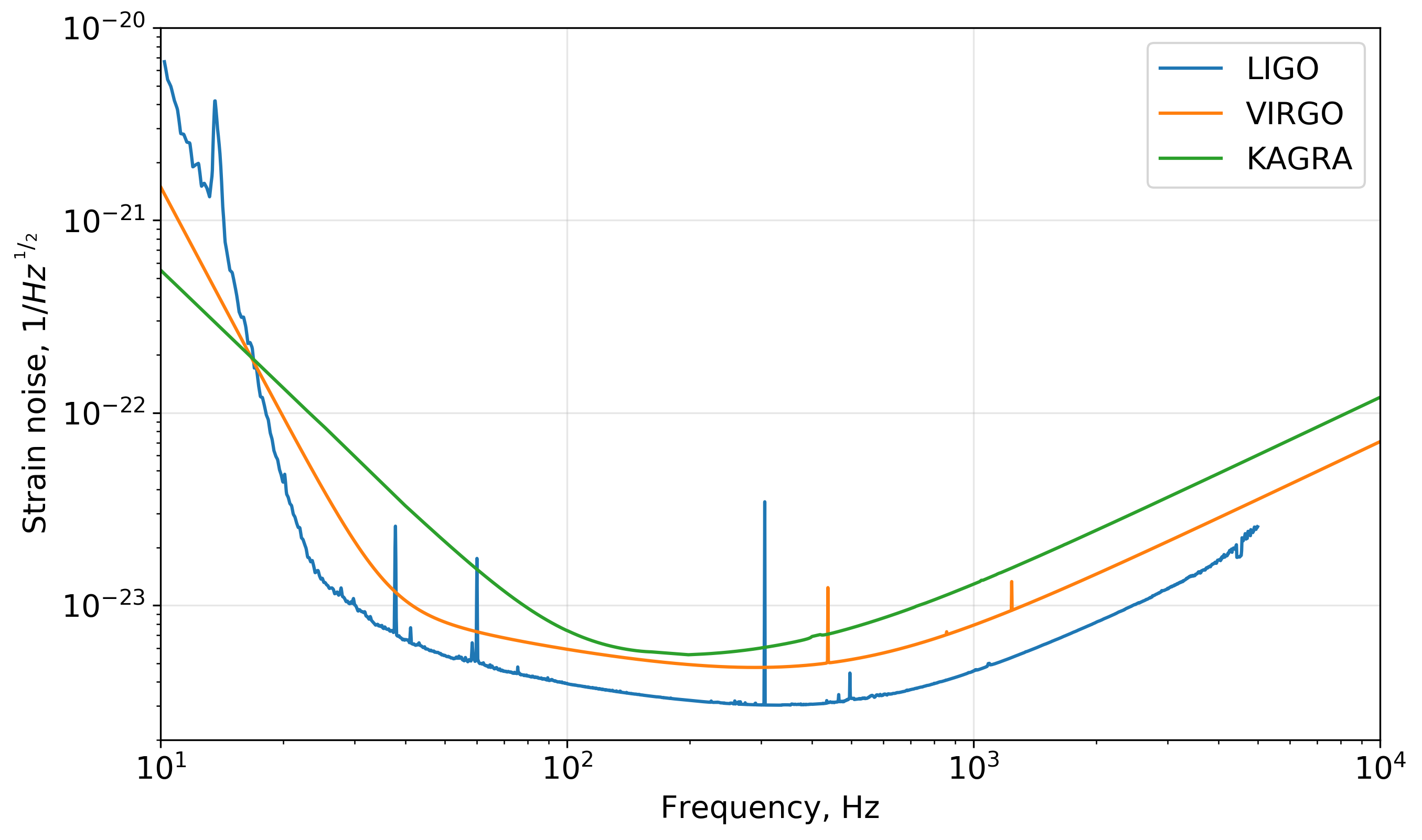
Figure 1: Projected LIGO, Virgo and KAGRA strain noise (i.e. amplitude spectral density), $\sqrt{S_{n}}$ as a function of frequency for the fourth observing run, O4. The data used to generate the noise curves above are retrieved from 2018LRR….21….3A .

To empirically test the Bayes factor scaling given by Equation 25, as well as investigate the effect on waveform reconstructions with detector networks of different sizes, we inject a set of simulated BBH signals into simulated detector noise and recover them using BayesWave. While BayesWave is a flexible algorithm that can detect a variety of signals from different sources, we use BBH waveforms as our test bed because they are well-understood sources, and have previously been used to study the performance of BayesWave 2016PhRvD..94d4050L ; 2017ApJ…839…15B ; 2020arXiv200309456G .

In this work, we use tools from the LIGO Analysis Library (lalsuite, ) to inject a set of non-spinning binary black holes (BBH) with equal component masses of $30M_{\odot}$. We use the phenomenological waveform IMRPhenomD to model spinning but non-precessing binaries using a combination of analytic post-Newtonian (PN), effective-one-body (EOB) and numerical relativity (NR) methods 2016PhRvD..93d4006H ; 2016PhRvD..93d4007K . The GW sources are distributed isotropically across the sky, and the inclinations $\iota$ are distributed uniformly in $\arccos{\iota}$. ${\rm SNR}_{\rm net}$ is distributed uniformly in SNR${}_{\text{net}}\in\{10,50\}$ where this SNR is calculated from a network comprising the HL detectors.

We inject 150 BBH signals into Gaussian noise coloured by the projected PSD of LIGO, Virgo and KAGRA for the fourth observing run, O4, as given in the LIGO, Virgo and KAGRA Observing Scenario 2018LRR….21….3A . The noise curves are shown in Figure 1.

We then recover the injected signals with BayesWave in three different scenarios: (i) Running only on Hanford and Livingston (HL) data (a two detector network), (ii) Running on the Hanford, Livingston, and Virgo (HLV) data (a three detector network) and (iii) Running on the Hanford, Livingston, KAGRA and Virgo (HLKV) data (a four detector network). All three detector configurations use the exact same injection data set.

In the two following sections, Sections A and B, we analyse two figures of merit: (i) Bayes factor and (ii) the overlap. By comparing these quantities between the HL and HLV networks, we can evaluate the performance of BayesWave in recovering the injected waveforms from detector networks of different sizes. As an extension to previous studies on sky localisation with expanded detector networks, we also compare the accuracy of BayesWave in recovering the sky location from detector networks of different sizes in Section C.

VI Results

A Recovered Bayes factors

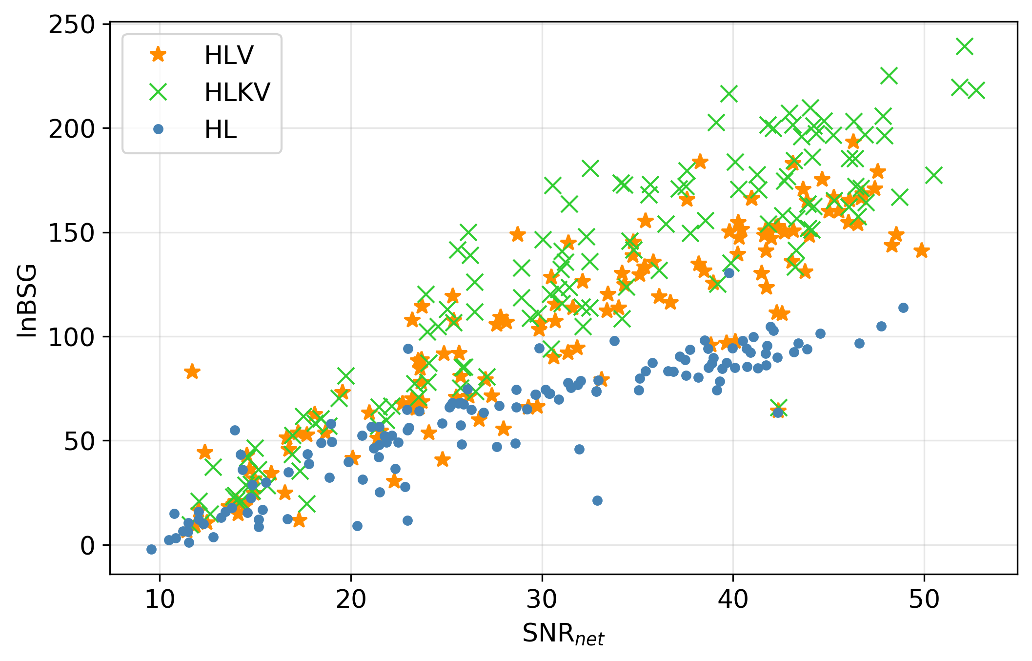
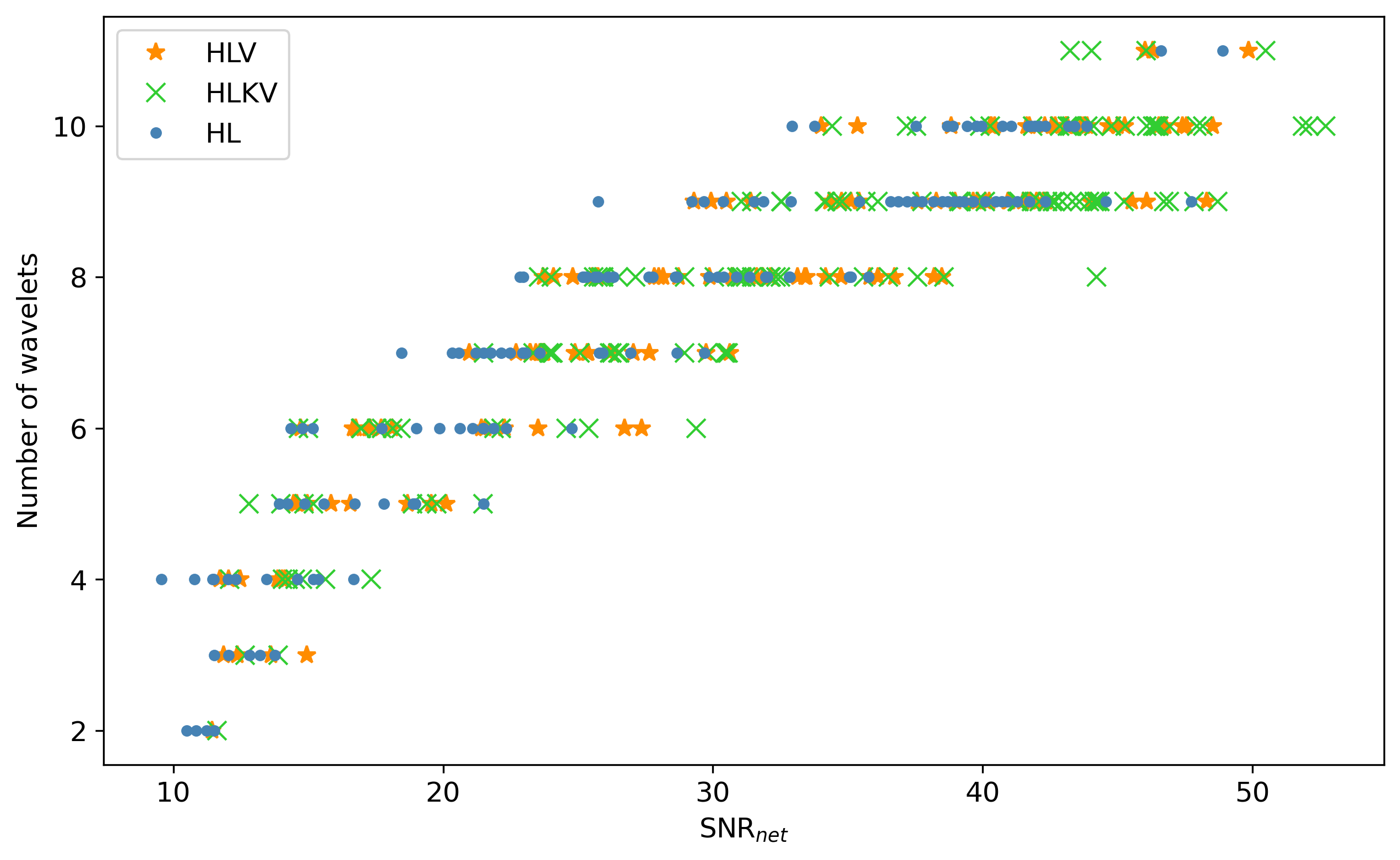
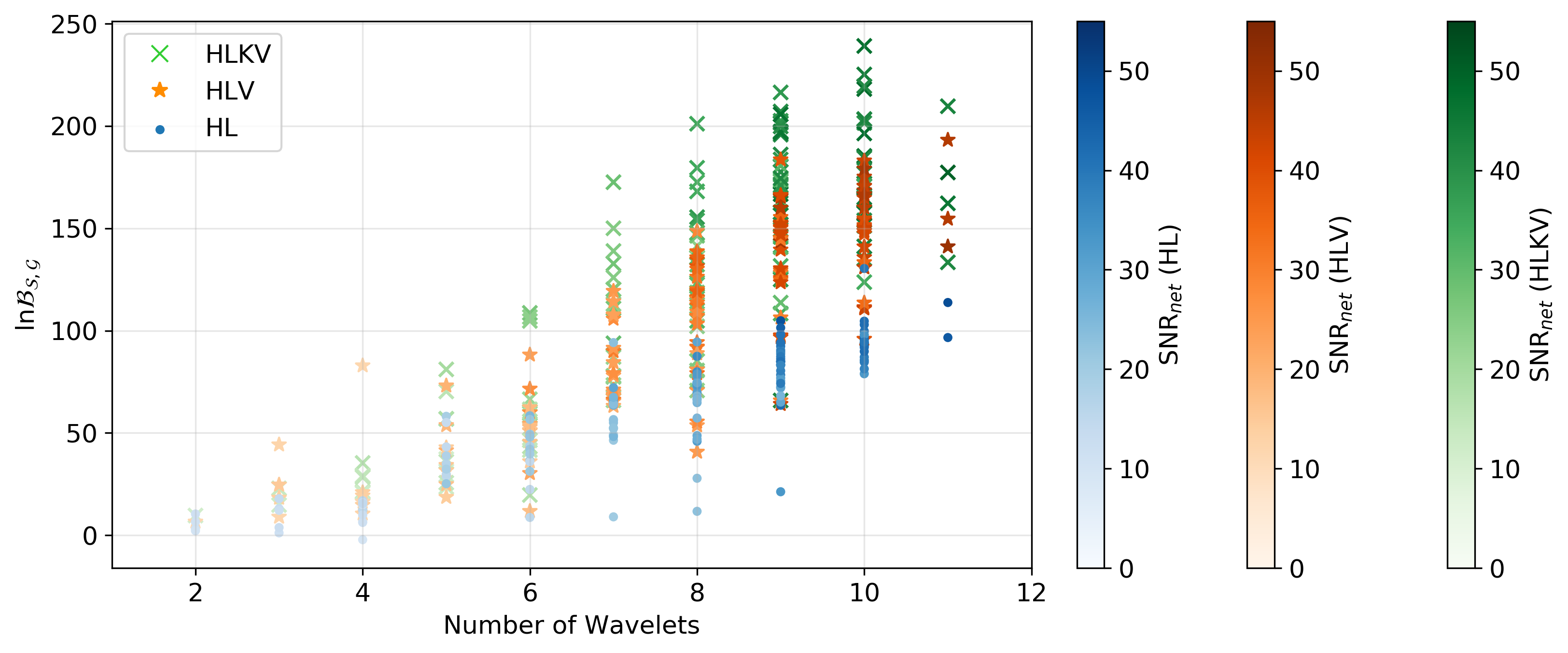
Figure 2: Top left panel shows the log signal-to-glitch Bayes Factor $\ln\mathcal{B}_{\mathcal{S},\mathcal{G}}$ of BBH injection recoveries versus network signal-to-noise ratio, SNR${}_{\text{net}}$. Each data point represents one BBH injection. Top right panel shows the median number of wavelets used in signal model reconstruction for each injection, $N$ versus SNR${}_{\text{net}}$. Bottom panel shows $\ln\mathcal{B}_{\mathcal{S},\mathcal{G}}$ versus $N$, and the three colour bars indicates the network SNR of each data point in the corresponding detector network. In the top panels, the horizontal axis corresponds three different network SNRs: (i) for the blue dot data points it corresponds to SNR${}_{\text{net}}$ of the HL network, (ii) for the orange star data points it corresponds to SNR${}_{\text{net}}$ of the HLV network, (iii) for the green cross data points it corresponds to SNR${}_{\text{net}}$ of the HLKV network.

After analysing the injections described in Section V, we use the model evidences calculated by BayesWave to understand the impact of GW detector network size on the log signal-to-glitch Bayes factor, $\ln\mathcal{B}_{\mathcal{S},\mathcal{G}}$. For all the analyses in this paper, we only injections that have been identified as inconsistent with Gaussian noise (this can be either a signal or glitch) by BayesWave. Injections indicated to be consistent with the Gaussian noise model ($\mathcal{N}$) by BayesWave are removed from the data set, since it would be meaningless to evaluate their respective signal and glitch model evidences. In other words, injections with $\ln\mathcal{B}_{\mathcal{S},\mathcal{N}}$ error bars encompassing values below zero are removed from the data set. The widths of $\ln\mathcal{B}_{\mathcal{S},\mathcal{N}}$ error bars are given by 2015CQGra..32m5012C

$$\Delta[\ln\mathcal{B}_{\mathcal{S},\mathcal{N}}]=\sqrt{\{\Delta[\ln p\left(d\,\middle|\,\mathcal{S}\right)]\}^{2}+\{\Delta[\ln p\left(d\,\middle|\,\mathcal{N}\right)]\}^{2}}$$ (27)

where $\Delta[\ln p\left(d\,\middle|\,\mathcal{M}\right)]$ is the uncertainty for the logarithmic evidence of model $\mathcal{M}$. A total of 14 data points are removed under this constraint. These events are all low SNR${}_{\text{net}}$ injections.

The top left panel of Figure 2 shows $\ln\mathcal{B}_{\mathcal{S},\mathcal{G}}$ as a function of SNR${}_{\text{net}}$ for the HL, HLV and HLKV networks. All three networks show a clear trend of increasing Bayes Factor with increasing network SNR as expected. Our results also show that the HLKV injections have the highest SNR overall, agreeing with Equation 4 which indicates that increasing $\mathcal{I}$ increases $\mathrm{SNR}_{\mathrm{net}}$. Furthermore, we can see that injections at comparable SNRs are recovered with higher $\ln\mathcal{B}_{\mathcal{S},\mathcal{G}}$ in the HLV network than the HL network. In other words, even after accounting for the increased SNR, we observe further enhancement in detection confidence for an expanded detector network, suggesting that $\ln\mathcal{B}_{\mathcal{S},\mathcal{G}}$ is related to $\mathcal{I}$, and not just the SNR of the signal as predicted by Equation 25.

The top right panel of Figure 2 shows the median number of wavelets used in the BayesWave reconstruction, $N$ versus the injected SNR in the respective detector networks, SNR${}_{\text{net}}$. The median here refers to the median of posterior distribution for $N$. We see that $N$ increases systematically with SNR${}_{\text{net}}$ in both the HL and HLV networks. This is expected since the detectors are able to pick up more complex features of the waveform at high SNR. At low SNR (SNR $\lesssim 15$) there is a slight deviation from the linear trend described by Equation 6 between $N$ and SNR in both detector networks. This is primarily due to the prior on the number of wavelets. This prior is determined empirically from runs in LIGO data after O1, and peaks around $N=3$ BWIII . $N$ also depends on waveform morphology and complexity 2016PhRvD..94d4050L ; 2018PhRvD..97j4057M . Injecting the same set of BBH waveforms into all three detector configurations result in similar trends between $N$ and SNR${}_{\text{net}}$.

Equation 25 shows that $\ln\mathcal{B}_{\mathcal{S},\mathcal{G}}$ also scales with the number of wavelets used in the reconstruction. Hence we also show empirically how the dimensionality of signal model (i.e. the number of wavelets) also contributes to the increase in $\ln\mathcal{B}_{\mathcal{S},\mathcal{G}}$ for different $\mathcal{I}$. We show this in the bottom panel of Figure 2 by plotting $\ln\mathcal{B}_{\mathcal{S},\mathcal{G}}$ versus $N$. Colour bars indicate the SNR${}_{\text{net}}$ of each data point. For all three detector configurations, $\ln\mathcal{B}_{\mathcal{S},\mathcal{G}}$ generally increases with $N$, as predicted by Equation 25. At low SNRs (i.e. SNR$<15$), detector networks recover the waveform with $N\leq 3$ and $\ln\mathcal{B}_{\mathcal{S},\mathcal{G}}\leq 50$ because low SNR injections have low amplitude features which are harder to reconstruct resulting in lower detection confidence. It is clear for injections recovered with $N>3$ that $\ln\mathcal{B}_{\mathcal{S},\mathcal{G}}$ in the HLKV network are generally higher than that of the HL and HLV networks at comparable $N$ and SNR${}_{\text{net}}$. This again emphasizes the point that the Bayes factor scales with $\mathcal{I}$.

A more thorough investigation of the relation between the empirical and analytic Bayes factor can be found in Appendix C, where we use a simplified injection set of single sine-Gaussian wavelets. By recovering sine-Gaussian wavelets with sine-Gaussian wavelets, Equation 6 reduces to $N=1$. The results show that the empirical scaling of the Bayes factor with $\mathcal{I}$ agrees with the analytical scaling in Equation 25 to a good approximation.

In summary, we show by comparing Bayes Factors between the HL, HLV and HLKV networks that expanding detector networks increases detection confidence. Our empirical results are consistent with the analytic results discussed Section IV, viz. $\ln\mathcal{B}_{\mathcal{S},\mathcal{G}}\propto\mathcal{I}N\ln\mathrm{SNR}_{\mathrm{net}}$. Heuristically, this can be understood via Occam’s razor: if coincident identical glitches are unlikely in two detectors, they are even more unlikely in three or more detectors. Therefore when identical waveforms are detected simultaneously across larger networks, they have a higher likelihood of being a signal.

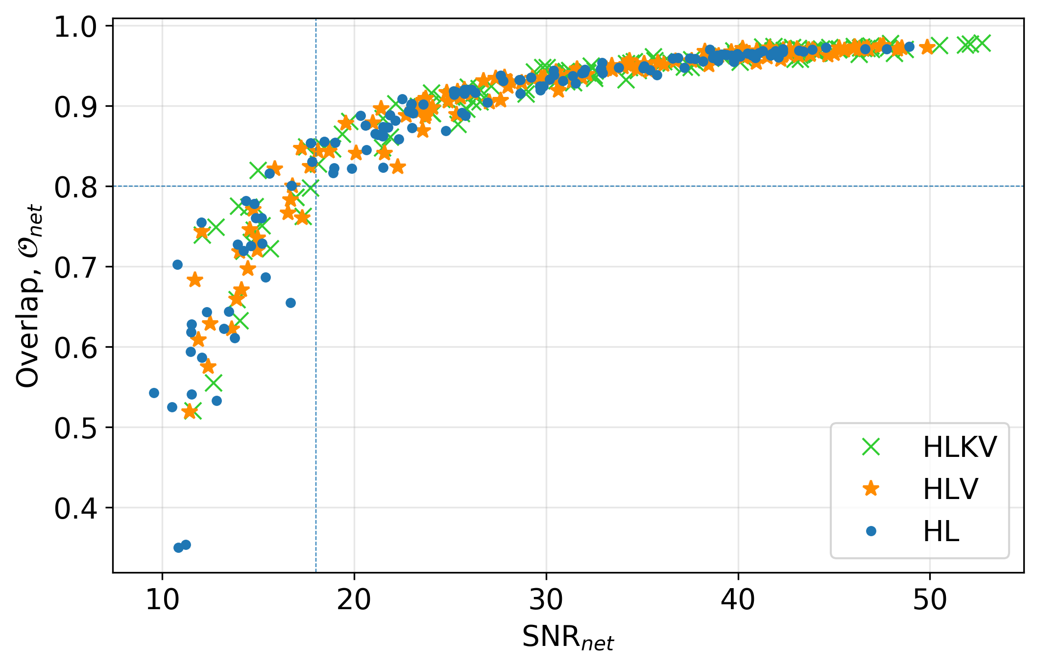
Figure 3: Median overlap between the injected and recovered waveform, $\mathcal{O}_{\text{net}}$ of the HL (blue dot) and HLV (orange star) network, as a function of SNR${}_{\text{net}}$. The horizontal blue line indicates $\mathcal{O}_{\text{net}}=0.8$ and the vertical blue line indicates SNR${}_{\text{net}}>15$.

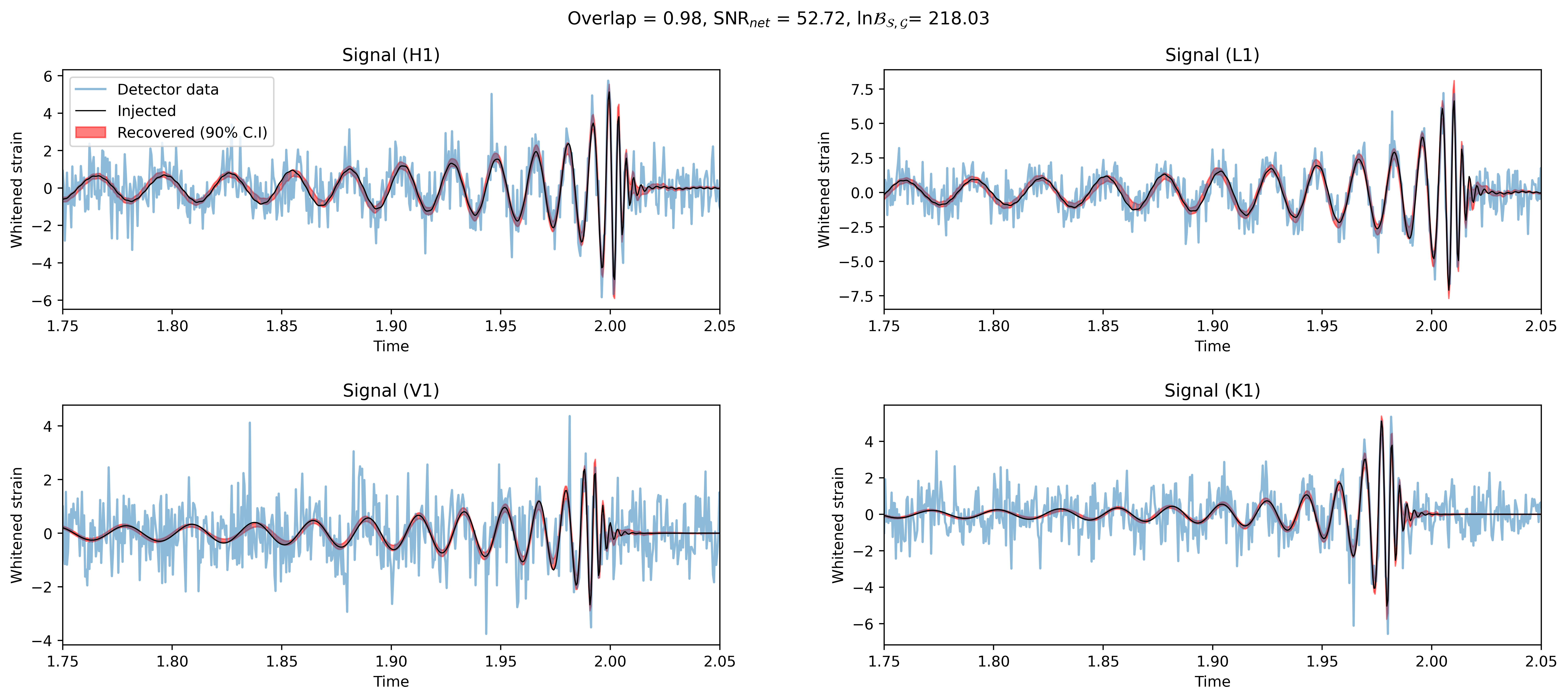
Figure 4: The top panel shows, for an injection with SNR${}_{\text{net}}=11.61$ and $\mathcal{O}=0.52$, the injected waveform (black), the detector data (blue) and the $90\%$ credible interval of the recovered waveform (red) for each detector in the HLKV network. Similarly in the bottom panel but for an injection with SNR${}_{\text{net}}=52.72$ and $\mathcal{O}=0.98$.

B Recovered Waveform Overlap

In the previous section, we showed that for a set of BBH waveforms, $\ln\mathcal{B}_{\mathcal{S},\mathcal{G}}$ increases with a larger number of detectors in the network, meaning with more detectors our confidence in detection is strengthened. In this section, we quantify the accuracy of BayesWave in waveform recovery by comparing the overlap (also sometimes called the match) between the injected and recovered waveforms for the HL, HLV and HLKV detector networks. The network overlap, $\mathbb{O}_{net}$ is given by Equation 13. For the rest of this paper, any mention of overlap refers to the network overlap.

Figure 3 shows the median overlap, $\mathbb{O}_{net}$ as a function of network SNR, where $\mathbb{O}_{net}$ of all three detector networks show positive correlation with their respective network SNR. This observation is consistent with previous results, which show that network overlap scales with SNR 2018PhRvD..97j4057M ; 2020arXiv200309456G . To illustrate how waveform reconstruction improves with SNR, Figure 4 shows the injected waveform (black), the detector data (blue) and the $90\%$ credible interval of the recovered waveform (red) for two events in the HLKV network. The top and bottom panels show the waveforms for the injection recovered with the smallest overlap ($\mathbb{O}_{\text{min}}=0.52$) and largest overlap ($\mathbb{O}_{\text{max}}=0.98$) of the whole injection data set respectively. The event with the smallest overlap has SNR${}_{\text{net}}=11.6$ and was recovered with $\ln\mathcal{B}_{\mathcal{S},\mathcal{G}}=9.66$, while the event with the largest overlap has SNR${}_{\text{net}}=52.72$ and was recovered with $\ln\mathcal{B}_{\mathcal{S},\mathcal{G}}=218.0$ This is consistent with the observed trend between overlap and network SNR in Figure 3. The similar trend between overlap and network SNR between all three detector configurations indicates that waveform reconstruction fidelity is not directly related to the number of detectors in the network.

However as noted earlier, increasing the number of detectors does increase the network SNR. By comparing the percentage of waveforms recovered with overlap above a given threshold for all three detector configurations, we show that having an additional detector allows us to better reconstruct the signal waveform. The threshold is arbitrarily defined here to be $\mathbb{O}_{\text{net}}>0.8$ and is indicated by the horizontal blue line in Figure 3. We found that $81\%$ of the injections were recovered with $\mathbb{O}_{\text{net}}>0.8$ for the HL network, $86\%$ for the HLV network and $87\%$ for the HLKV network.

While the inclusion of additional detector(s) does not have an extra benefit in the same way it does for the Bayes factor as shown in the previous section, it nonetheless allows us to better reconstruct the signal waveform due to increased SNR. However, the improvement is less significant upon the addition of KAGRA, since it is less sensitive compared to Virgo as shown in Figure 1 and therefore the increase in SNR is less compared to when Virgo is added to the network. The overall results also show that BayesWave is able to reconstruct waveforms reasonably well with all three detector configurations for injections with SNR${}_{\text{net}}>18$ as indicated by the vertical blue line in Figure 3.

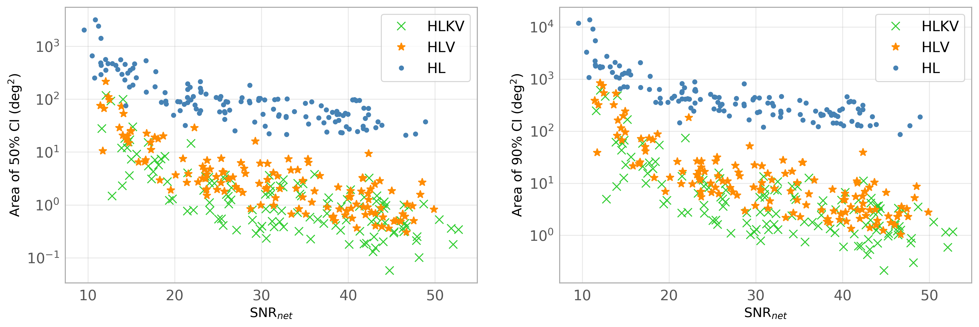
Figure 5: The left panel shows the sky area enclosed within the $50\%$ credible interval (CI) in square degrees versus the network SNR of the corresponding detector network. Similarly on the right panel, except for the $90\%$ CI.

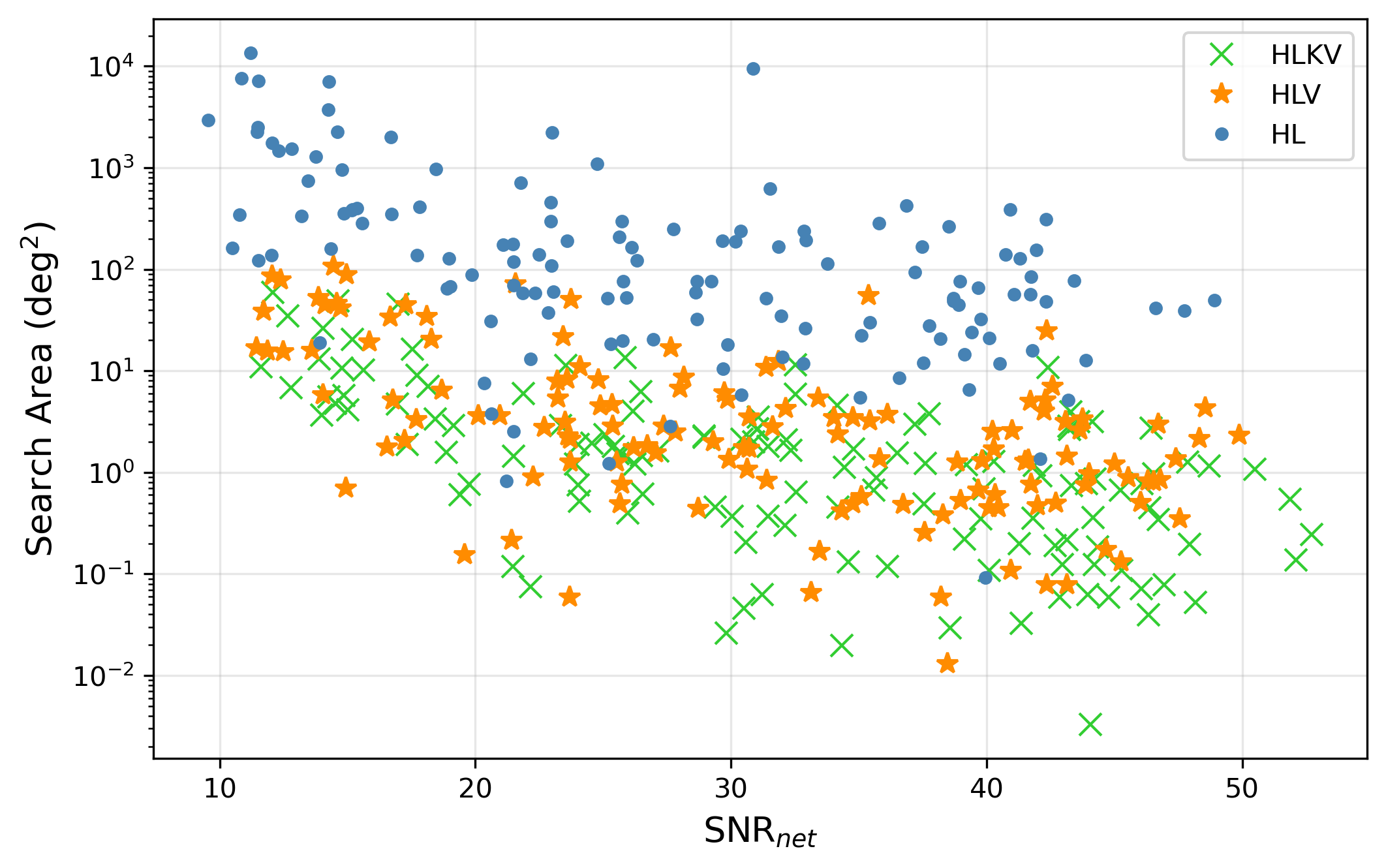
Figure 6: Search area, $\mathcal{A}$ (Equation 28) versus network SNR for the HL (blue dots) and HLV (orange stars) networks.

C Sky localisation

Expanding detector networks improves sky localisation of GW events, as has been shown by various studies on coherent network detections e.g 2011CQGra..28l5023S 2018ApJ…854L..25P and 2019PhRvD.100l4003P ; see Section II. In this section, we compare the accuracy of BayesWave in locating the source with the HL and HLV networks. We use two separate measures: (i) sky area enclosed within the $50\%$ and $90\%$ credible intervals (CI) and (ii) search area, $\mathcal{A}$.

For every injection, BayesWave produces posterior distributions for the sky location (in the form of right ascension and declination) of the GW signal. We first look at the sky area enclosed within $50\%$ and $90\%$ credible intervals (CIs) of the posterior distribution of source location. In the left panel of Figure 5, we show the plot for sky area enclosed within the $50\%$ CI versus network SNR for each injection, and similarly for the the $90\%$ CI on the right panel. For all three detector configurations, we note that the area within the $50\%$ and $90\%$ CIs measured in square degrees (deg²) fundamentally reduces with increasing network SNR due to improved accuracy in arrival time differences 2018ApJ…854L..25P . However, both sky areas are generally an order of magnitude smaller for the HLV network compared to the HL network. Upon addition of the KAGRA detector, we observe further reduction in the sky area, but not as drastic as that between the HL and HLV networks since KAGRA is less sensitive than Virgo. The areas enclosed within both $50\%$ and $90\%$ CIs reduces with increasing $\mathcal{I}$ due to the additional arrival time differences which further constrain the location of each source. These results reiterate that accuracy of sky localisation improves at fixed CI as $\mathcal{I}$ increases.

We also compare the inferred sky location with the true injected location of the source. We introduce another metric - the search area, $\mathcal{A}$, the hypothetical sky area observed by a detector before it correctly points towards the true location. To define this quantity mathematically, we first denote the posterior probability density function (PDF) of sky location as $p_{\text{sky}}(\phi,\theta)$. If the true location of the source is $(\phi_{t},\theta_{t})$ and $p_{0}=p_{\text{sky}}(\phi_{t},\theta_{t})$, then all points within $\mathcal{A}$ should have $p_{\text{sky}}\geq p_{0}$. Mathematically, we write 2015ApJ…800…81E ; 2017ApJ…839…15B

$$\mathcal{A}=\int H[p_{\text{sky}}(\phi,\theta)-p_{0}]\,d\Omega$$ (28)

where $H$ is the Heaviside step function and $d\Omega$ is the surface area element on the celestial sphere i.e. $d\Omega=\cos\delta d\theta d\phi$. In Figure 6 we plot the search area, $\mathcal{A}$ against network SNR for both the HL and HLV networks. The HLVK search area is slightly smaller than the HLV search area, which in turn is significantly smaller than the HL search area, consistent with Figure 5.

Overall, we see that sky localisation improves remarkably when a detector of high-sensitivity is added to the network. If a less sensitive detector is added, the improvements are small but not negligible.

VII Conclusion

The aim of this study is to compare the performance of BayesWave in recovering GW waveforms from detector networks of different sizes. We derive an analytic scaling for the Bayes factor between the signal and glitch models, $\mathcal{B}_{\mathcal{S},\mathcal{G}}$. We then inject a set of simulated BBH signals of fixed masses at different SNRs into simulated O4 detector data of the HL, HLV and HLKV network. We quantify BayesWave’s performance in signal identification with $\mathcal{B}_{\mathcal{S},\mathcal{G}}$ and the performance in waveform reconstruction with overlap, $\mathcal{O}_{\text{net}}$. We also compare the accuracy of sky localisation between the two networks.

We find that events of similar injected SNR analysed using the HLV and HLKV network have higher $\ln\mathcal{B}_{\mathcal{S},\mathcal{G}}$ than those using the HL network. This agrees with theoretical prediction of the Bayes factor scaling:

$$\ln\mathcal{B}_{\mathcal{S},\mathcal{G}}\propto\mathcal{I}N\ln\text{SNR}_{\text{net}}.$$ (29)

Previous work 2016PhRvD..94d4050L demonstrated that BayesWave is unique amongst GW umodelled burst searches in that the so-called “complexity” of the signal in time-frequency plane plays a crucial role in the detection statistic, rather than just the signal’s strength. This is understood through the factor of $N$ in Equation 29: a signal with more complex structure needs more wavelets to accurately reconstruct the waveform. In this work, we expose another novel feature of the BayesWave algorithm: the detection statistic is also influenced by the number of detectors i.e. the factor of $\mathcal{I}$ in Equation 29. Events of similar injected SNR (SNR${}_{\text{net}}$) analysed using larger detector networks have higher $\ln\mathcal{B}_{\mathcal{S},\mathcal{G}}$, indicating detection confidence increases more than we would expect purely from the increase in SNR${}_{\text{net}}$.

The network overlap, $\mathcal{O}_{\text{net}}$, between the injected and recovered waveforms increases with SNR${}_{\text{net}}$. We also show that $87\%$ of the HLKV network, $86\%$ of the HLV network and $81\%$ of the HL network injections have $\mathcal{O}>0.8$. Since larger detector networks can detect signals at higher SNR, they pick up more details of the true waveform. Thus, BayesWave can reconstruct the waveforms more accurately.

Finally in Section C, we quantify accuracy of sky localisation with the sky area enclosed within the $50\%$ and $90\%$ credible intervals (CI). We find that both areas decrease with increasing SNR${}_{\text{net}}$ and are generally an order of magnitude smaller for the HLV networks than the HL network. The reduction of sky area is less significant upon the addition of the KAGRA detector due to its low sensitivity compared to Virgo. The search area, $\mathcal{A}$ also decreases with increasing SNR${}_{\text{net}}$ and increasing number of detectors. The overall results suggest that increasing the number of detectors at different geographical locations improves sky localisation, consistent with previous analyses 2011CQGra..28l5023S ; 2018ApJ…854L..25P ; 2019PhRvD.100l4003P .

With the global detector network growing in size, the outlook for improving detection confidence with unmodelled burst searches is promising. Prospective work along the lines of the research presented in this paper may include injecting different waveform morphologies to compare detection confidence between detector networks of different sizes. We also recommend looking into quantifying and comparing the outcomes of BayesWave in recovering simulated signals from more realistic detector noise (i.e. in the presence of glitches) between different detector configurations.

In summary, BayesWave shows significant improvements in terms of waveform recovery and parameter estimation when working with a larger detector network. This promising result suggests that with more detectors joining the global network in the future, we will be able to reconstruct generic GW burst signals more accurately using BayesWave making detections with higher Bayes factor and hence with higher confidence.

Appendix A Fisher Information Matrix

Each wavelet has its Fisher Information Matrices (FIMs), $\Gamma$ written in terms of its five intrinsic parameters $\{t_{0},f_{0},Q,\ln A,\phi_{0}\}$

$$\Gamma=\text{SNR}^{2}\begin{pmatrix}\frac{4\pi^{2}f_{0}^{2}(1+Q^{2})}{Q^{2}}&0&0&0&-2\pi f_{0}\\ 0&\frac{3+Q^{2}}{4f_{0}^{2}}&-\frac{3}{4Qf_{0}}&-\frac{1}{2f_{0}}&0\\ 0&-\frac{3}{4Qf_{0}}&\frac{3}{4Q^{2}}&\frac{1}{2Q}&0\\ 0&-\frac{1}{2f_{0}}&\frac{1}{2Q}&1&0\\ -2\pi f_{0}&0&0&0&1\end{pmatrix}_{.}$$ (30)

FIMs contain information on local curvature of the likelihood of wavelet parameters which accelerates convergence by proposing jumps in the MCMC algorithm towards regions of higher likelihood 2015CQGra..32m5012C . BayesWave uses FIMs to update wavelet parameters by drawing proposals from a multivariate Gaussian distribution

$$q(\mathbf{y}|\mathbf{x})=\frac{\det\Gamma}{(2\pi)^{2}}\exp\left(-\frac{1}{2}\Gamma_{ij}\Delta x^{i}\Delta x^{j}\right)$$ (31)

where $\Delta x^{i}=x^{i}-y^{i}$ denotes the displacement in intrinsic parameter $i$ before and after the update.

Appendix B Assumptions for Bayes Factor Scaling

Laplace approximations for the logarithmic signal ($\mathcal{S}$) and glitch ($\mathcal{G}$) model evidences are given by Equations 23 and 24 respectively. In order to see how $\mathcal{B}_{\mathcal{S},\mathcal{G}}$ scales with the waveform parameters, we make some assumptions to simplify the two logarithmic evidences. In this work we use the same assumptions as in Ref. 2016PhRvD..94d4050L .

Loud signals typically have optimal extrinsic parameters across the detector network, so the SNR in each detector will be approximately equal such that

$$\text{SNR}_{i,n}\approx\frac{\text{SNR}_{\text{net},n}}{\sqrt{\mathcal{I}}}$$ (32)

where $\text{SNR}_{i,n}$ is the SNR of the $n$-th wavelet in detector $i$. We use a further simplifying assumption that the SNR of each wavelet is the same

$$\text{SNR}_{\text{net},n}\approx\frac{\text{SNR}_{\text{net}}}{\sqrt{N}},$$ (33)

which has been empirically validated. We assume that the glitch model in each detector uses similar reconstruction parameters as the signal model, and as such the quality factors of all wavelets are approximately equal:

$$Q^{\mathcal{G}}_{i,n}\approx Q^{\mathcal{S}}_{n}\equiv Q$$ (34)

and similarly,

$$N^{\mathcal{G}}\approx N^{\mathcal{S}}\equiv N.$$ (35)

Recall that $N^{\mathcal{G}}$ indicates the number of wavelets used in the glitch model for a single detector, so for an $\mathcal{I}$-detector network, the total number of wavelets used in glitch models across the entire network is $\mathcal{I}N$.

Equations 23 and 24 can be simplified to

$$\ln p\left(d\,\middle|\,\mathcal{S}\right)\simeq\frac{\text{SNR}_{\text{net}}^{2}}{2}-\frac{5N}{2}-N\ln(V_{\lambda})+\sum_{n=1}^{N}\ln\left(\bar{Q}_{n}\right)-5N\ln(\frac{\text{SNR}_{\text{net}}}{\sqrt{N}})+\left(2+\ln\frac{\sqrt{\det C_{\Omega}}}{V_{\Omega}}\right)$$ (36)

$$\ln p\left(d\,\middle|\,\mathcal{G}\right)\simeq\frac{\text{SNR}_{\text{net}}^{2}}{2}-\mathcal{I}\left[\frac{5N}{2}+N\ln(V_{\lambda})-\sum_{n=1}^{N}\ln\left(\bar{Q}_{n}\right)+5N\ln(\frac{\text{SNR}_{\text{net}}}{\sqrt{N\mathcal{I}}})\right].$$ (37)

Appendix C Scaling of Bayes factor with $\mathcal{I}$

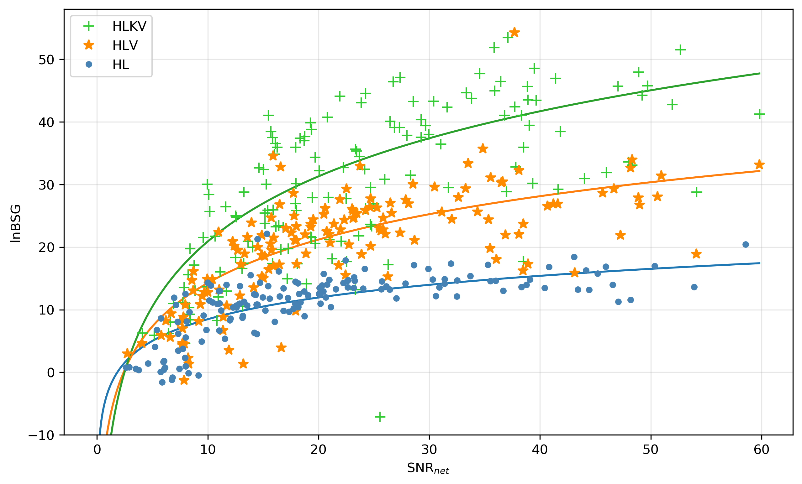
Figure 7: Log signal-to-glitch Bayes factor, $\ln\mathcal{B}_{\mathcal{S},\mathcal{G}}$ of sine-Gaussian wavelet recoveries versus network signal-to-noise ratio, SNR${}_{\text{net}}$. The solid lines with colours corresponding to the data symbols are analytic predictions of $\ln\mathcal{B}_{\mathcal{S},\mathcal{G}}$ given by Equation 39.

Our results in Section A show that $\ln\mathcal{B}_{\mathcal{S},\mathcal{G}}$ scales with SNR, $N$, and $\mathcal{I}$. As per Equation 6, $N$ itself depends on both the SNR of the signal, and the waveform morphology. In order to specifically test the scaling of $\ln\mathcal{B}_{\mathcal{S},\mathcal{G}}$ with $\mathcal{I}$ alone, we inject a set of sine-Gaussian wavelets as coherent signals into detector noise for the HL, HLV and HLKV network and then recover them using BayesWave. Because sine-Gaussian wavelets are the basis of reconstruction for BayesWave, the number of wavelets used is $N=1$, with no dependence on SNR.

The dataset used this analysis is a set of 150 single sine-Gaussian wavelets. The parameters of each wavelet are randomly drawn from the following distributions: $t_{0}\in[1.5,2.5]$ s (where $t=1\ {\rm s}$ is the center of the analysis window), $f_{0}\in[32,1000]$ Hz, $Q\in[0.1,40]$ and $\phi_{0}\in[0,2\pi]$. The SNR of the signals are drawn randomly from a uniform distribution and SNR $\in[10,50]$, and the amplitude is then found viz.

$$A=\text{SNR}\sqrt{\frac{2\sqrt{2\pi}f_{0}S_{n}(f_{0})}{Q}}$$ (38)

(see 2018PhRvD..97j4057M for details). As we are injecting a coherent signal, we also require four extrinsic parameters as described in Section A. These parameters are also drawn randomly from uniform distributions such that $\alpha\in[0,2\pi]$, $\delta\in[-\nicefrac{{\pi}}{{2}},\nicefrac{{\pi}}{{2}}]$, $\psi\in[0,2\pi]$ and $\epsilon\in[-0.99,0.99]$.

In Figure 7, we plot $\ln\mathcal{B}_{\mathcal{S},\mathcal{G}}$ of each injection against ${\rm SNR}_{\text{net}}$ for the HL, HLV and HLKV network injections. We note that $\ln\mathcal{B}_{\mathcal{S},\mathcal{G}}$ increases with SNR${}_{\text{net}}$ and is generally higher for networks with greater $\mathcal{I}$, as predicted from Equation 26. Since $N$ in this case does not depend on SNR, we can be certain that the differences in $\ln\mathcal{B}_{\mathcal{S},\mathcal{G}}$ between the different detector configurations at comparable SNR${}_{\text{net}}$ are entirely due to $\mathcal{I}$.

In order to compare the analytic and empirical scaling of $\ln\mathcal{B}_{\mathcal{S},\mathcal{G}}$ with $\mathcal{I}$, we fit analytic approximation of $\ln\mathcal{B}_{\mathcal{S},\mathcal{G}}$ for each detector network with a generalised expression

$$\ln\mathcal{B}_{\mathcal{S},\mathcal{G}}\approx(\mathcal{I}-1)[5\ln\text{SNR}_{\text{net}}+a]+\frac{5}{2}\mathcal{I}\ln\mathcal{I}+b.$$ (39)

This expression is derived from Equation 25 with $N=1$. We define the constants $a=\frac{5}{2}-\ln(V_{\lambda})+\ln(Q)$ and $b=2+\ln\frac{\sqrt{\det C_{\Omega}}}{V_{\Omega}}$. The prior volumes, $V_{\lambda}$ and $V_{\Omega}$ are respectively the same for all detector configurations. We do not have an analytic expression for $\det C_{\Omega}$ as the FIM approximations is inadequate; the extrinsic parameter space contains degeneracy between parameters, resulting in multimodal, non-Gaussian likelihood distribution which spans the full extent of the prior range (see 2016PhRvD..94d4050L for details). We present the fits as three solid lines in Figure 7, where we have determined by-eye $a=-10$ and $b=4$. The same values of $a$ and $b$ are used for all three fits and they are broadly consistent with the empirical results.

We see general agreement between the empirical results and predicted scaling for $\ln\mathcal{B}_{\mathcal{S},\mathcal{G}}$, which further confirms our results in Section A that the Bayes factor does not only depend on SNR${}_{\text{net}}$ but also on $\mathcal{I}$. We again note that these scalings are estimations, and due to the different sensitivities of the detectors we do not expect exact agreement between analytic prediction and empirical results.

References

- [1] J Aasi, B P Abbott, R Abbott, T Abbott, et al. Advanced LIGO. Classical and Quantum Gravity, 32(7):074001, mar 2015.
- [2] B. P. Abbott, R. Abbott, R. Adhikari, P. Ajith, et al. LIGO: the Laser Interferometer Gravitational-Wave Observatory. Reports on Progress in Physics, 72(7):076901, July 2009.
- [3] Gregory M Harry. Advanced LIGO: the next generation of gravitational wave detectors. Classical and Quantum Gravity, 27(8):084006, apr 2010.
- [4] B. P. Abbott, R. Abbott, T. D. Abbott, et al. All-sky search for short gravitational-wave bursts in the first Advanced LIGO run. Phys. Rev. D, 95(4):042003, February 2017.
- [5] B. P. Abbott, R. Abbott, T. D. Abbott, et al. GWTC-1: A Gravitational-Wave Transient Catalog of Compact Binary Mergers Observed by LIGO and Virgo during the First and Second Observing Runs. Physical Review X, 9(3):031040, July 2019.
- [6] B. P. Abbott, R. Abbott, T. D. Abbott, et al. All-sky search for short gravitational-wave bursts in the second Advanced LIGO and Advanced Virgo run. Phys. Rev. D, 100(2):024017, July 2019.
- [7] Iulia Georgescu. O3 highlights. Nature Reviews Physics, 2(5):222–223, April 2020.
- [8] F. Acernese, M. Agathos, K. Agatsuma, D. Aisa, N. Allemandou, et al. Advanced Virgo: a second-generation interferometric gravitational wave detector. Classical and Quantum Gravity, 32(2):024001, January 2015.
- [9] T. Akutsu, M. Ando, K. Arai, et al. First cryogenic test operation of underground km-scale gravitational-wave observatory KAGRA. Classical and Quantum Gravity, 36(16):165008, August 2019.
- [10] T. Akutsu, M. Ando, K. Arai, Y. Arai, et al. Overview of KAGRA: Detector design and construction history. arXiv e-prints, page arXiv:2005.05574, May 2020.
- [11] Yoichi Aso, Yuta Michimura, Kentaro Somiya, Masaki Ando, Osamu Miyakawa, Takanori Sekiguchi, Daisuke Tatsumi, and Hiroaki Yamamoto. Interferometer design of the KAGRA gravitational wave detector. Phys. Rev. D, 88(4):043007, August 2013.
- [12] Chris L. Fryer and Kimberly C. B. New. Gravitational Waves from Gravitational Collapse. Living Reviews in Relativity, 14(1):1, January 2011.
- [13] Elan Stopnitzky and Stefano Profumo. Gravitational Waves from Gamma-Ray Pulsar Glitches. ApJ, 787(2):114, June 2014.
- [14] Thibault Damour and Alexander Vilenkin. Gravitational radiation from cosmic (super)strings: Bursts, stochastic background, and observational windows. Phys. Rev. D, 71(6):063510, March 2005.
- [15] L. Blackburn, L. Cadonati, S. Caride, S. Caudill, S. Chatterji, et al. The LSC glitch group: monitoring noise transients during the fifth LIGO science run. Classical and Quantum Gravity, 25(18):184004, September 2008.
- [16] J. Aasi, J. Abadie, B. P. Abbott, R. Abbott, T. Abbott, et al. Characterization of the LIGO detectors during their sixth science run. Classical and Quantum Gravity, 32(11):115012, June 2015.
- [17] J. Aasi, J. Abadie, B. P. Abbott, R. Abbott, T. D. Abbott, et al. The characterization of Virgo data and its impact on gravitational-wave searches. Classical and Quantum Gravity, 29(15):155002, August 2012.
- [18] Samantha A. Usman, Alexander H. Nitz, Ian W. Harry, et al. The PyCBC search for gravitational waves from compact binary coalescence. Classical and Quantum Gravity, 33(21):215004, November 2016.
- [19] Surabhi Sachdev, Sarah Caudill, Heather Fong, et al. The GstLAL Search Analysis Methods for Compact Binary Mergers in Advanced LIGO’s Second and Advanced Virgo’s First Observing Runs. arXiv e-prints, page arXiv:1901.08580, January 2019.
- [20] Shaun Hooper, Shin Kee Chung, Jing Luan, David Blair, Yanbei Chen, and Linqing Wen. Summed parallel infinite impulse response filters for low-latency detection of chirping gravitational waves. Phys. Rev. D, 86(2):024012, July 2012.
- [21] Ryan Lynch, Salvatore Vitale, Reed Essick, Erik Katsavounidis, and Florent Robinet. Information-theoretic approach to the gravitational-wave burst detection problem. Phys. Rev. D, 95(10):104046, May 2017.
- [22] S. Klimenko, I. Yakushin, A. Mercer, and G. Mitselmakher. A coherent method for detection of gravitational wave bursts. Classical and Quantum Gravity, 25(11):114029, June 2008.
- [23] Tyson B. Littenberg and Neil J. Cornish. Bayesian inference for spectral estimation of gravitational wave detector noise. Phys. Rev. D, 91(8):084034, April 2015.
- [24] Neil J. Cornish and Tyson B. Littenberg. Bayeswave: Bayesian inference for gravitational wave bursts and instrument glitches. Classical and Quantum Gravity, 32(13):135012, July 2015.
- [25] Neil J. Cornish, Tyson B. Littenberg, Bence Bécsy, Katerina Chatziioannou, James A. Clark, Sudarshan Ghonge, and Margaret Millhouse. BayesWave analysis pipeline in the era of gravitational wave observations. Phys. Rev. D, 103(4):044006, February 2021.
- [26] Tyson B. Littenberg, Jonah B. Kanner, Neil J. Cornish, and Margaret Millhouse. Enabling high confidence detections of gravitational-wave bursts. Phys. Rev. D, 94(4):044050, August 2016.
- [27] Jonah B. Kanner, Tyson B. Littenberg, Neil Cornish, Meg Millhouse, Enia Xhakaj, Francesco Salemi, Marco Drago, Gabriele Vedovato, and Sergey Klimenko. Leveraging waveform complexity for confident detection of gravitational waves. Phys. Rev. D, 93(2):022002, January 2016.
- [28] C. S. Unnikrishnan. IndIGO and Ligo-India Scope and Plans for Gravitational Wave Research and Precision Metrology in India. International Journal of Modern Physics D, 22(1):1341010, January 2013.
- [29] Curt Cutler and Éanna E. Flanagan. Gravitational waves from merging compact binaries: How accurately can one extract the binary’s parameters from the inspiral waveform? Phys. Rev. D, 49(6):2658–2697, March 1994.
- [30] Drew Garvin Keppel. Signatures and Dynamics of Compact Binary Coalescences and a Search in LIGO’s S5 Data. PhD thesis, California Institute of Technology, April 2009.
- [31] S. M. Gaebel and J. Veitch. How would GW150914 look with future gravitational wave detector networks? Classical and Quantum Gravity, 34(17):174003, September 2017.
- [32] Bence Bécsy, Peter Raffai, Neil J. Cornish, et al. Parameter Estimation for Gravitational-wave Bursts with the BayesWave Pipeline. ApJ, 839(1):15, April 2017.
- [33] Hsin-Yu Chen and Daniel E. Holz. The Loudest Gravitational Wave Events. arXiv e-prints, page arXiv:1409.0522, September 2014.
- [34] Bernard F. Schutz. Networks of gravitational wave detectors and three figures of merit. Classical and Quantum Gravity, 28(12):125023, June 2011.
- [35] Alessandro Manzotti and Alexander Dietz. Prospects for early localization of gravitational-wave signals from compact binary coalescences with advanced detectors. arXiv e-prints, page arXiv:1202.4031, February 2012.
- [36] Chris Pankow, Eve A. Chase, Scott Coughlin, et al. Improvements in Gravitational-wave Sky Localization with Expanded Networks of Interferometers. ApJ, 854(2):L25, February 2018.
- [37] W. Del Pozzo, C. P. L. Berry, A. Ghosh, T. S. F. Haines, L. P. Singer, and A. Vecchio. Dirichlet process Gaussian-mixture model: An application to localizing coalescing binary neutron stars with gravitational-wave observations. MNRAS, 479(1):601–614, September 2018.
- [38] Margaret Millhouse, Neil J. Cornish, and Tyson Littenberg. Bayesian reconstruction of gravitational wave bursts using chirplets. Phys. Rev. D, 97(10):104057, May 2018.
- [39] Jordan B. Camp and Neil J. Cornish. Gravitational Wave Astronomy. Annual Review of Nuclear and Particle Science, 54:525–577, December 2004.
- [40] Tyson B. Littenberg and Neil J. Cornish. Bayesian approach to the detection problem in gravitational wave astronomy. Phys. Rev. D, 80(6):063007, September 2009.
- [41] Markus Abt and William J. Welch. Fisher information and maximum-likelihood estimation of covariance parameters in gaussian stochastic processes. Canadian Journal of Statistics, 26(1):127–137, 1998.
- [42] Joseph D. Romano and Neil. J. Cornish. Detection methods for stochastic gravitational-wave backgrounds: a unified treatment. Living Reviews in Relativity, 20(1):2, April 2017.
- [43] Tyson B. Littenberg. A comprehensive Bayesian approach to gravitational wave astronomy. PhD thesis, Montana State University, April 2009.
- [44] B. P. Abbott, R. Abbott, T. D. Abbott, et al. Prospects for observing and localizing gravitational-wave transients with Advanced LIGO, Advanced Virgo and KAGRA. Living Reviews in Relativity, 21(1):3, April 2018.
- [45] Sudarshan Ghonge, Katerina Chatziioannou, James A. Clark, Tyson Littenberg, Margaret Millhouse, Laura Cadonati, and Neil Cornish. Reconstructing gravitational wave signals from binary black hole mergers with minimal assumptions. arXiv e-prints, page arXiv:2003.09456, March 2020.
- [46] LIGO Scientific Collaboration. LIGO Algorithm Library - LALSuite. free software (GPL), 2018.
- [47] Sascha Husa, Sebastian Khan, Mark Hannam, Michael Pürrer, Frank Ohme, Xisco Jiménez Forteza, and Alejandro Bohé. Frequency-domain gravitational waves from nonprecessing black-hole binaries. I. New numerical waveforms and anatomy of the signal. Phys. Rev. D, 93(4):044006, February 2016.
- [48] Sebastian Khan, Sascha Husa, Mark Hannam, Frank Ohme, Michael Pürrer, Xisco Jiménez Forteza, and Alejandro Bohé. Frequency-domain gravitational waves from nonprecessing black-hole binaries. II. A phenomenological model for the advanced detector era. Phys. Rev. D, 93(4):044007, February 2016.
- [49] Hsing-Po Pan, Chun-Yu Lin, Zhoujian Cao, and Hwei-Jang Yo. Accuracy of source localization for eccentric inspiraling binary mergers using a ground-based detector network. Phys. Rev. D, 100(12):124003, December 2019.
- [50] Reed Essick, Salvatore Vitale, Erik Katsavounidis, Gabriele Vedovato, and Sergey Klimenko. Localization of Short Duration Gravitational-wave Transients with the Early Advanced LIGO and Virgo Detectors. ApJ, 800(2):81, February 2015.