Simultaneous Mode, State and Input Set-Valued Observers for Switched Nonlinear Systems

Abstract

In this paper, we study the problem of designing a simultaneous mode, input and state set-valued observer for a class of hidden mode switched nonlinear systems with bounded-norm noise and unknown input signals, where the hidden mode and unknown inputs can represent fault or attack models and exogenous fault/disturbance or adversarial signals, respectively. The proposed multiple-model design has three constituents: (i) a bank of mode-matched set-valued observers, (ii) a mode observer and (iii) a global fusion observer. The mode-matched observers recursively find the sets of compatible states and unknown inputs conditioned on the mode being the true mode, while the mode observer eliminates incompatible modes by leveraging a residual-based criterion. Then, the global fusion observer outputs the estimated sets of states and unknown inputs by taking the union of the mode-matched set-valued estimates over all compatible modes. Moreover, sufficient conditions to guarantee the elimination of all false modes (i.e., mode detectability) are provided and the effectiveness of our approach is demonstrated and compared with existing approaches using an illustrative example.

1 Introduction

Cyber-Physical Systems (CPS), which tightly couple communication and computation elements, can enhance the functionality of control systems and improve their performance. However, these features may also become a source of vulnerability to attacks or faults. On the other hand, autonomous systems, e.g., self-driving cars or robots, typically must operate without the direct knowledge of the intentions and decisions of other systems/agents. These systems, which can be conveniently considered within the general framework of hidden mode hybrid/switched systems (HMHS, see, e.g., [1, 2, 3] and references therein) with unknown inputs, are often safety-critical. Thus, the ability to estimate the states, unknown inputs and modes of such systems is important for monitoring these systems as well as for designing feedback controllers with safety and security guarantees.

Literature review. The problem of designing filters/observers for hidden mode systems, without considering unknown inputs/faults/data injection attacks, has been extensively studied, e.g., in [4, 5] and references therein. Recently, the work in [2, 3] proposed an extension to include unknown inputs for stochastic systems, aiming to obtain point estimates, i.e., the most likely or best single estimates. However, probabilistic distributions of uncertainty are often unavailable and moreover, it may also be desirable to consider set-valued uncertainties, e.g., bounded-norm noise, especially when hard guarantees or bounds are important. In the latter setting, set-membership or set-valued state observers, e.g., [6, 7, 8], have been proposed to estimate the set of compatible states, and later, extensions of this framework to include the estimation of unknown inputs have been proposed in [9, 10, 11]. Nonetheless, these approaches are not directly applicable to systems with hidden modes that are considered in this paper.

To consider hidden modes, which can be used to model/represent fault or attack models, a common approach is to construct residual signals (see, e.g., [2, 3, 4, 12, 13, 14]), where a threshold based on the residual signal is used to distinguish between consistent and inconsistent modes. In the context of resilient state estimation against sparse data injection attacks, [15] presented a robust control-inspired approach for linear systems with bounded-norm noise that consists of local estimators, residual detectors, and a global fusion detector. Similar residual-based techniques have been used for uniformly observable nonlinear systems in [16] and some classes of nonlinear systems in [17]. However, these approaches only consider sparse attacks on the sensors, which is a special case of a hidden mode system, as was discussed in our previous work for hidden mode switched linear stochastic systems in [2]. Thus, to our best knowledge, the design of an estimator for hidden mode switched nonlinear systems with unknown inputs and bounded-norm noise remains an open problem.

Contributions. To bridge this gap, this paper considers the problem of simultaneous mode, state and unknown input estimation for hidden mode switched nonlinear systems with bounded-norm noise, where the hidden mode represents a fault or attack model. To tackle this problem, our preliminary conference publication [18] proposed a multiple-model approach for switched linear systems. In this paper, we further extend this approach to hidden mode switched nonlinear systems with unknown inputs using a similar multiple-model approach, which consists of a bank of mode-matched set-valued observers and a novel elimination-based mode observer. The mode-matched set-valued observers are based on the optimally designed set-valued state and input $\mathcal{H}_{\infty}$ observers in our recent work [11], while the mode observer eliminates inconsistent modes from the bank of observers by using the upper bound of the norm of to-be-designed residual signals as a threshold. In particular, we propose a tractable method to calculate an upper bound signal for the residual’s norm by carefully over-approximating the value function of a non-concave NP-hard norm-maximization problem with a convex maximization problem over a convex set that has a finite number of extreme points in a manner that guarantees that no compatible modes are eliminated. We also prove that the upper bound signal is a convergent sequence. Furthermore, we provide sufficient conditions for mode detectability, i.e., for guaranteeing that all false modes will be eventually ruled out under some reasonable assumptions. Finally, we compare the performance of our proposed approach with an existing $\mathcal{H}_{\infty}$ observer in the literature.

Notation. $\mathbb{R}^{n}$ denotes the $n$-dimensional Euclidean space, and $\mathbb{N}$ the set of nonnegative integers. For a vector $v\in\mathbb{R}^{n}$, $\|v\|_{2}\triangleq\sqrt{v^{\top}v}$ and $\|v\|_{\infty}\triangleq\max\limits_{1\leq i\leq n}v_{i}$, and for a matrix $M\in\mathbb{R}^{p\times q}$, $\|M\|_{2}$, $\sigma_{\min}(M)$ and $M(i:j)$ denote the induced $2$-norm, the smallest non-trivial singular value and the sub-matrix consisting of the $i$-th through $j$-th columns of $M$, respectively. Further, $0_{n\times m}$ denotes an $n$-by-$m$ zero matrix.

2 Problem Statement

Consider a hidden mode switched nonlinear system with bounded-norm noise and unknown inputs (i.e., a hybrid system with nonlinear and noisy system dynamics in each mode, where the mode and some inputs are not known/measured):

$$\begin{array}[]{ll}x_{k+1}&=f^{q}(x_{k})+B^{q}u^{q}_{k}+G^{q}d^{q}_{k}+W^{q}w^{q}_{k},\\ y_{k}&=C^{q}x_{k}+D^{q}u^{q}_{k}+H^{q}d^{q}_{k}+v^{q}_{k},\end{array}$$ (3)

where $x_{k}\in\mathbb{R}^{n}$ is the continuous system state and $q\in\mathbb{Q}=\{1,2,\dots,Q\}\subset\mathbb{N}$ is the hidden discrete state or mode. For each $q\in\mathbb{Q}$, $y_{k}\in\mathbb{R}^{l}$ is the measurement output signal and $w^{q}_{k}\in\mathbb{R}^{n}$ and $v^{q}_{k}\in\mathbb{R}^{l}$ are external process and measurement disturbances with known $\ell_{2}$-norm bounds, i.e., $\|w_{k}\|_{2}\leq\eta_{w}$ and $\|v_{k}\|_{2}\leq\eta_{v}$, respectively. Moreover, $u^{q}_{k}\in U_{k}\subset\mathbb{R}^{m}$ is the known input and $d^{q}_{k}\in\mathbb{R}^{p}$ the unknown input signal (representing, e.g., the input of other agents/robots or adversarially injected data signal). It is worth mentioning that no prior ‘useful’ knowledge or assumption of the dynamics of $d^{q}_{k}$ is assumed. For each (fixed) mode $q$, the mapping $f^{q}(\cdot):\mathbb{R}^{n}\to\mathbb{R}^{n}$ and the matrices $B^{q}\in\mathbb{R}^{n\times m}$, $G^{q}\in\mathbb{R}^{n\times p}$, $C^{q}\in\mathbb{R}^{l\times n}$, $D^{q}\in\mathbb{R}^{l\times m}$ and $H^{q}\in\mathbb{R}^{l\times p}$ are the corresponding mode-dependent known state vector field and system matrices, respectively.

The above modeling framework can capture a very broad range of problems, including intention estimation, fault detection and resilient state estimation against sparse data injection and switching/mode attacks. Specifically, in the context of intention estimation or fault diagnosis, each mode represents an intent or fault model and the unknown inputs can model the inputs of other agents/robots or exogenous fault signals. On the other hand, with regard to resilient state estimation, the switching/mode attacks (e.g., attacks on circuit breakers) can be represented with a set of different $f^{q}(\cdot)$, $B^{q}$, $C^{q}$ and $D^{q}$, while the unknown attack location of sparse data injection attacks can be modeled by a set of different $G^{q}$ and $H^{q}$ that represent the different hypotheses for which actuators and sensors are attacked or not attacked. Further, the attack signal magnitudes can be modeled as the unknown inputs in this scenario.

In addition, we assume the following:

Assumption 1.

There is only one “true” mode, i.e. the true mode $q^{*}$ is constant over time.

Assumption 2.

For each $q\in\mathbb{Q}$, $f^{q}(\cdot)$ is twice continuously differentiable and Lipschitz continuous on its domain with a known Lipschitz constant $L^{q}_{f}>0$.

Using the above modeling framework, the simultaneous state, unknown input and hidden mode estimation problem based on a multiple-model framework can be stated as follows:

Problem 1.

Given a hidden mode switched nonlinear discrete-time system with unknown inputs and bounded-norm noise in the form of (3),

1. Design a bank of mode-matched observers, where each mode-matched observer, conditioned on the mode being true, optimally returns the set -valued estimates of compatible states and unknown inputs in the minimum $\mathcal{H}_{\infty}$-norm sense, i.e., with minimum average power amplification.

2. Find a threshold criterion to eliminate false modes and subsequently, develop a mode observer via elimination.

3. Derive sufficient conditions for the elimination of all false modes.

3 Proposed Observer Design

In this section, we propose a multiple-model approach for simultaneous mode, state and unknown input estimation for the system in (3), with the goal of recursively finding the sets of states $\hat{X}_{k}$, unknown inputs $\hat{D}_{k}$ and modes $\hat{\mathbb{Q}}_{k}$ that are compatible with observed outputs $y_{k}$.

3.1 Overview of Multiple-Model Approach

The multiple-model design approach consists of three steps: (i) designing a bank of mode-matched set-valued observers, (ii) developing a mode observer for eliminating incompatible modes using a residual-based threshold, and (iii) devising a global fusion observer that returns the desired set-valued mode, input and state estimates.

3.1.1 Mode-Matched Set-Valued Observer

First, based on the optimal fixed-order observer design in [11], we develop a bank of mode-matched observers, which includes $Q\in\mathbb{N}$ simultaneous state and input $\mathcal{H}_{\infty}$ set-valued observers, which can be briefly summarized as follows. For each mode-matched observer corresponding to mode $q$, following the approach in [11, Section 4], we consider set-valued fixed-order estimates in the form of $\ell_{2}$-norm balls:

$$\hat{D}^{q}_{k-1} =\{d_{k-1}\in\mathbb{R}^{p}:\|d_{k-1}-\hat{d}^{q}_{k-1}\|{\color[rgb]{0,0,0}_{2}}\leq\delta^{d,q}_{k-1}\},$$ (4)

$$\hat{X}^{q}_{k} =\{x_{k}\in\mathbb{R}^{n}:\|x_{k}-\hat{x}^{q}_{k|k}\|{\color[rgb]{0,0,0}_{2}}\leq\delta^{x,q}_{k}\},$$ (5)

where their centroids $\hat{x}^{q}_{k|k}$ and $\hat{d}^{q}_{k-1}$ are obtained with the following three-step recursive observer that is optimal in $\mathcal{H}_{\infty}$-norm sense (cf. [11, Section 4.2] for more details):

Unknown Input Estimation:

$$\begin{array}[]{rl}\hat{d}^{q}_{1,k}&=M^{q}_{1}(z^{q}_{1,k}-C^{q}_{1}\hat{x}^{q}_{k|k}-D^{q}_{1}u^{q}_{k}),\\ \hat{d}^{q}_{2,k-1}&=M^{q}_{2}(z^{q}_{2,k}-C^{q}_{2}\hat{x}^{q}_{k|k-1}-D^{q}_{2}u^{q}_{k}),\\ \hat{d}^{q}_{k-1}&=V^{q}_{1}\hat{d}^{q}_{1,k-1}+V^{q}_{2}\hat{d}^{q}_{2,k-1};\end{array}$$ (9)

Time Update:

$$\begin{array}[]{rl}\hat{x}^{q}_{k|k-1}&=f^{q}(\hat{x}^{q}_{k-1|k-1})+B^{q}u^{q}_{k-1}+G^{q}_{1}\hat{d}^{q}_{1,k-1},\\ \hat{x}^{\star,q}_{k|k}&=\hat{x}^{q}_{k|k-1}+G^{q}_{2}\hat{d}^{q}_{2,k-1};\end{array}$$ (12)

Measurement Update:

$$\hat{x}^{q}_{k|k} =\hat{x}^{\star,q}_{k|k}+\tilde{L}^{q}(z^{q}_{2,k}-C^{q}_{2}\hat{x}^{\star,q}_{k|k}-D^{q}_{2}u^{q}_{k}),\quad$$ (13)

where $C^{q}_{1}$, $C^{q}_{2}$, $D^{q}_{1}$, $D^{q}_{2}$, $G^{q}_{1}$, $G^{q}_{2}$, $V^{q}_{1}$, $V^{q}_{2}$, $z^{q}_{1,k}$ and $z^{q}_{2,k}$ can be computed by applying a similarity transformation described in A and $\tilde{L}^{q}\in\mathbb{R}^{n\times(l-p_{H^{q}})}$, $M^{q}_{1}\in\mathbb{R}^{p_{H^{q}}\times p_{H^{q}}}$ and $M^{q}_{2}\in\mathbb{R}^{(p-p_{H^{q}})\times(l-p_{H^{q}})}$ are observer gain matrices that are chosen via the following Proposition 1. This proposition is a restatement of the results in [11] that is tailored to the setting considered in this paper, where the main idea is to minimize the “volume” of the set of compatible states and unknown inputs, quantified by the radii $\delta^{d,q}_{k-1}$ and $\delta_{k}^{x,q}$.

Proposition 1.

[11, Proposition 5.16, Lemma 5.1 & Theorem 5.13] Consider system (3) and a bank of $Q$ mode-matched observers in the form of (9)–(13). Suppose that $\forall q\in\mathbb{Q}\triangleq\{1,\dots,Q\}$, ${\rm rk}(C^{q}_{2}G^{q}_{2})=p-p_{H^{q}}$ and $M^{q}_{1},M^{q}_{2}$ are chosen as $M^{q}_{1}=(\Sigma^{q})^{-1}$ and $M^{q}_{2}=(C^{q}_{2}G^{q}_{2})^{\dagger}$, where $\Sigma^{q}$ is obtained by applying singular value decomposition on $H^{q}$ (cf. A for more details). Then, the following statements hold:

1. Given mode $q\in\mathbb{Q}$, the following difference equation governs the state estimation error dynamics (i.e., the dynamics of $\tilde{x}^{q}_{k|k}\triangleq x_{k}-\hat{x}^{q}_{k|k}$):

   $$\tilde{x}^{q}_{k+1|k+1}=(I-\tilde{L}^{q}C^{q}_{2})\Phi^{q}(\Delta f_{k}^{q}-\Psi^{q}\tilde{x}^{q}_{k|k})+\mathcal{W}^{q}(\tilde{L}^{q})\overline{w}^{q}_{k},$$ (14)

   where

   $$\Delta f^{q}_{k} \triangleq f^{q}(x_{k})-f^{q}(\hat{x}^{q}_{k}),\quad\Phi^{q}\triangleq I-G^{q}_{2}M^{q}_{2}C^{q}_{2},$$

   $$\overline{w}^{q}_{k} \triangleq\begin{bmatrix}(\frac{1}{\sqrt{2}})v^{q\top}_{k}&w^{q\top}_{k}&(\frac{1}{\sqrt{2}})v^{q\top}_{k+1}\end{bmatrix}^{\top},$$

   $$R^{q} \triangleq\begin{bmatrix}-\sqrt{2}\Phi^{q}G^{q}_{1}M^{q}_{1}T^{q}_{1}&-\Phi^{q}W^{q}&-\sqrt{2}G^{q}_{2}M^{q}_{2}T^{q}_{2}\end{bmatrix},$$

   $$Q^{q} \triangleq\begin{bmatrix}0_{(l-p_{H^{q}})\times l}&0_{(l-p_{H^{q}})\times n}&-\sqrt{2}T^{q}_{2}\end{bmatrix},$$

   $$\Psi^{q} \triangleq G^{q}_{1}M^{q}_{1}C^{q}_{1},\quad\mathcal{W}^{q}(\tilde{L}^{q})\triangleq(I-\tilde{L}^{q}C^{q}_{2})R^{q}+\tilde{L}^{q}Q^{q}.$$

2. Solving the following mixed-integer SDP for each mode $q$:

   $$(\rho^{\star}_{q})^{2}=\min_{\{P\succ 0,\Gamma\succ 0,\tilde{\Gamma}\succeq 0,\breve{Q}\succeq 0,Y,\breve{Z},\rho^{2}>0,0\leq\alpha\leq 1,\varepsilon_{1}>0,\varepsilon_{2}>0,{\kappa>0},\kappa_{1}>0,\kappa_{2}>0\}}\rho^{2}$$

   $$s.t.\begin{bmatrix}P&\tilde{Y}^{q}_{1}\\ \tilde{Y}^{q\top}_{1}&\tilde{\mathbf{M}}^{q}_{1}\end{bmatrix}\succeq 0,\begin{bmatrix}P&\tilde{Y}^{q}_{2}\\ \tilde{Y}^{q\top}_{2}&\tilde{\mathbf{M}}^{q}_{2}\end{bmatrix}\succeq 0,\begin{bmatrix}P&\tilde{Y}^{q}_{1}\\ \tilde{Y}^{q\top}_{1}&\tilde{\mathbf{M}}^{q}_{3}\end{bmatrix}\succeq 0,$$

   $$\quad\ \begin{bmatrix}P&\tilde{Y}^{q}_{2}\\ \tilde{Y}^{q\top}_{2}&\ \breve{Z}\end{bmatrix}\succeq 0,\ \ \begin{bmatrix}\tilde{\Gamma}&\breve{Z}\\ \breve{Z}^{\top}&\Psi^{q\top}\breve{Q}\Psi^{q}\end{bmatrix}\succeq 0,$$

   $$\quad\ \begin{bmatrix}I-\Gamma&0&0\\ 0&P&Y\\ 0&Y^{\top}&I\end{bmatrix}\succeq 0,\ \begin{bmatrix}\mathcal{N}^{q}_{11}&*&*\\ \mathcal{N}^{q}_{21}&\mathcal{N}^{q}_{22}&*\\ \mathcal{N}^{q}_{31}&0&\mathcal{N}^{q}_{33}\end{bmatrix}\succeq 0,$$

   $$\quad\ \ \kappa_{1}I\preceq P\preceq\kappa_{2}I,\ \land\ ((\kappa_{1}\geq 1,\kappa_{2}-\kappa_{1}<1)\ \vee\ (\kappa_{2}\leq 1,\kappa_{1}>0.5)),$$

   we obtain an observer in the form of (9)–(13) with the observer gain $\tilde{L}^{q}=(P^{q})^{-1}Y^{q}$, where $(P^{q},Y^{q})$ are solutions to the above mixed-integer SDP, that

   • is quadratically stable, and

   • guarantees that

     $$\theta^{q}\triangleq\|(I-\tilde{L}^{q}C^{q}_{2})\Phi^{q}\|{\color[rgb]{0,0,0}_{2}}<1,$$ (15)

     and consequently, the upper bound sequences for the radii $\{{\delta}^{x,q}_{k},{\color[rgb]{0,0,0}^{d,q}_{k-1}}\}_{k=1}^{\infty}$, which are computed as:

     $$\begin{array}[]{ll}{\delta}^{x,q}_{k}&\triangleq\delta^{x}_{0}{\color[rgb]{0,0,0}(\theta^{q})}^{k}+\overline{\eta}^{q}\frac{1-{{\color[rgb]{0,0,0}(\theta}^{q})}^{k}}{1-\theta^{q}},\\ {\delta}^{d}_{k-1}&\triangleq\beta^{q}{\delta}^{x,q}_{k-1}+\overline{\alpha}^{q},\end{array}$$ (18)

     are convergent to some steady state value ${\delta}^{x,q}_{\infty},{\color[rgb]{0,0,0}^{d,q}_{\infty}}$ (cf. B for definitions of ${\delta}^{x,q}_{\infty}$ and ${\color[rgb]{0,0,0}^{d,q}_{\infty}}$, as well as the matrices and parameters in the above SDP and (18)).

3.1.2 Mode Observer

To estimate the set of compatible modes, we consider an elimination approach that compares the $\ell_{2}$-norm of residual signals against some thresholds. Specifically, we will eliminate a specific mode $q$, if $\|r^{q}_{k}\|_{2}>\hat{\delta}^{q}_{r,k}$, where the residual signal $r^{q}_{k}$ is defined as follows and the thresholds $\hat{\delta}^{q}_{r,k}$ will be derived in Section 3.2.

Definition 1 (Residuals).

For each mode $q$ at time step $k$, the residual signal is defined as:

$$r^{q}_{k}\triangleq z^{q}_{2,k}-C^{q}_{2}\hat{x}^{\star,q}_{k|k}-D^{q}_{2}u^{q}_{k}.$$

3.1.3 Global Fusion Observer

Finally, combining the outputs of both components above, our proposed global fusion observer will provide mode, unknown input and state set-valued estimates at each time step $k$ as:

$$\begin{array}[]{c}\hat{\mathbb{Q}}_{k}=\{q\in\mathbb{Q}\ \vline\ \|r^{q}_{k}\|_{2}\leq\hat{\delta}^{q}_{r,k}\},\\ \hat{D}_{k-1}=\cup_{q\in\hat{\mathbb{Q}}_{k}}D^{q}_{k-1},\ \hat{X}_{k}=\cup_{q\in\hat{\mathbb{Q}}_{k}}X^{q}_{k}.\end{array}$$

The multiple-model approach is summarized in Algorithm 1.

Algorithm 1 Simultaneous Mode, State and Input Estimation

1:$\hat{\mathbb{Q}}_{0}=\mathbb{Q}$;

2:for $k=1$ to $N$ do

3:    for $q\in\hat{\mathbb{Q}}_{k-1}$ do

4:$\triangleright$ Mode-Matched State and Input Set-Valued Estimates

5:     Compute $T^{q}_{2},M^{q}_{1},M^{q}_{2},\tilde{L}^{q},\hat{x}^{\star,q}_{k|k},\hat{X}^{q}_{k},\hat{D}^{q}_{k-1}$ via Proposition 1;

6:     $z^{q}_{2,k}=T^{q}_{2}y_{k}$;

7:$\triangleright$ Mode Observer via Elimination

8:     $\hat{\mathbb{Q}}_{k}=\hat{\mathbb{Q}}_{k-1}$;

9:     Compute $r^{q}_{k}$ via Definition 1 and $\hat{\delta}^{q}_{r,k}$ via Theorem 2;

10:         if $\|r^{q}_{k}\|_{2}>\hat{\delta}^{q}_{r,k}$ then $\hat{\mathbb{Q}}_{k}=\hat{\mathbb{Q}}_{k}\backslash\{q\}$;

11:         end if

12:    end for

13:$\triangleright$ State and Input Estimates

14:    $\hat{X}_{k}=\cup_{q\in\hat{\mathbb{Q}}_{k}}\hat{X}^{q}_{k}$;  $\hat{D}_{k}=\cup_{q\in\hat{\mathbb{Q}}_{k}}\hat{D}^{q}_{k}$;

15:end for

3.2 Mode Elimination Approach

We leverage a relatively simple idea to develop a criterion for elimination of false modes, as follows. We rule out a particular mode as incompatible, if the $\ell_{2}$-norm of its corresponding residual signal exceeds its upper bound conditioned on this mode being true. To do so, for each mode $q$, we first compute an upper bound ($\hat{\delta}^{q}_{r,k}$) for the $\ell_{2}$-norm of its corresponding residual at time $k$, conditioned on $q$ being the true mode. Then, comparing the $\ell_{2}$-norm of residual signal in Definition 1 with $\hat{\delta}^{q}_{r,k}$, mode $q$ can be eliminated if the residual’s $\ell_{2}$-norm is strictly greater than the upper bound. The following proposition and theorem formalize this procedure.

Proposition 2.

Consider mode $q$ at time step $k$, its residual signal $r^{q}_{k}$ (as defined in Definition 1) and the unknown true mode $q^{*}$. Then,

$$r^{q}_{k}=r^{q|*}_{k}+\Delta r^{q|q*}_{k},$$

with

$$r^{q|*}_{k}\triangleq z^{q*}_{2,k}-C^{q}_{2}\hat{x}^{\star,q}_{k|k}-D^{q}_{2}u^{q}_{k}=T^{q*}_{2}y_{k}-C^{q}_{2}\hat{x}^{\star,q}_{k|k}-D^{q}_{2}u^{q}_{k},$$

$$\Delta r^{q|q*}_{k}\triangleq(T^{q}_{2}-T^{q*}_{2})y_{k},$$

​​​​ where $r^{q|*}_{k}$ is the true mode’s residual signal (i.e., $q=q^{*}$), and $\Delta r^{q|q^{*}}_{k}$ is the residual error.

Proof.

This follows directly from plugging the above expressions into the right hand side term of Definition 1. ∎

Theorem 1.

Consider mode $q$ and its residual signal $r^{q}_{k}$ at time step $k$. Assume that $\delta^{q,*}_{r,k}$ is any signal that satisfies $\|r^{q|*}_{k}\|_{2}\leq\delta^{q,*}_{r,k}$, where $r^{q|*}_{k}$ is defined in Proposition 2. Then, mode $q$ is not the true mode, i.e., can be eliminated at time $k$, if $\|r^{q}_{k}\|_{2}>\delta^{q,*}_{r,k}.$

Proof.

To use contradiction, suppose that $\|r^{q}_{k}\|_{2}>\delta^{q,*}_{r,k}$ and let $q$ be the true mode, i.e., $q=q^{*}$ and thus, $T^{q}_{2}=T^{q*}_{2}$. By Proposition 2, $\Delta r^{q|q*}_{k}=0$ and hence, $\|r^{q}_{k}\|_{2}=\|r^{q|*}_{k}\|_{2}\leq\delta^{q,*}_{r,k}$, which contradicts with the assumption. ∎

By the above theorem, our approach guarantees that the true mode is never eliminated. However, Theorem 1 only provides a sufficient condition for mode elimination at each time step and the capability of our proposed mode observer to eliminate as many false modes as possible is dependent on the tightness of the upper bound, $\delta^{q,*}_{r,k}$.

3.3 Tractable Computation of Thresholds

To apply the sufficient condition in Theorem 1, we need a tractable approach to compute the upper bound $\delta^{q,*}_{r,k}$ that is finite-valued. This procedure is derived and described in the following.

Lemma 1.

Consider any mode $q$ with the unknown true mode being $q^{*}$. Then, at time step $k$, we have

$$r^{q|*}_{k} =C^{q}_{2}\tilde{x}^{\star,q}_{k|k}+v^{q}_{2,k}=\mathbb{A}^{q}_{k}{t}_{k},$$ (19)

where

$${t}_{k}\triangleq\begin{bmatrix}\tilde{x}^{\top}_{0|0}&v^{q\top}_{0}&\dots&v^{q\top}_{k}&w^{q\top}_{0}&\dots&w^{q\top}_{k-1}&\Delta f_{0}^{q\top}\dots\Delta f_{k-1}^{q\top}\end{bmatrix}^{\top}\in\mathbb{R}^{{(n+l)(k+1)+nk}},$$

$$\mathbb{A}^{q}_{k}\triangleq[A^{q}_{k}\ \ J^{q,1}_{k-1}\ \ (J^{q,2}_{k-1}+J^{q,1}_{k-2})\cdots(J^{q,2}_{1}+J^{q,1}_{0})\ \ J^{q,2}_{0}\ \ J^{q,3}_{k-1}\dots J^{q,3}_{0}\ \ F^{q}_{k-1}\dots F^{q}_{0}],$$

$$A^{q}_{k}\triangleq(-1)^{k}((I-\tilde{L}^{q}C^{q}_{2})\Phi^{q}\Psi^{q})^{k},$$

$$J^{q}_{i}\triangleq\begin{cases}\mathcal{Y}_{q},\hfill\text{if}\ i=0,\\ -C^{q}_{2}\Phi^{q}G^{q}_{1}M^{q}_{1}C^{q}_{1}(I-\tilde{L}^{q}C^{q}_{2})^{i-1}\mathcal{W}^{q},\quad\quad\quad\quad\quad\quad\quad\quad\quad\text{if}\ 1\leq i\leq k-1,\end{cases}$$

$$F^{q}_{i}\triangleq\begin{cases}C^{q}_{2}\Phi^{q},\quad\quad\quad\quad\quad\quad\quad\quad\quad\quad\quad\quad\quad\quad\quad\quad\quad\quad\quad\quad\quad\quad\quad\quad\ \text{if}\ i=0,\\ (-1)^{i}C^{q}_{2}\Phi^{q}G^{q}_{1}M^{q}_{1}C^{q}_{1}((I-\tilde{L}^{q}C^{q}_{2})\Psi^{q})^{i-1}(I-\tilde{L}^{q}C^{q}_{2})\Phi^{q},\ \ \text{if}\ 1\leq i\leq k-1,\end{cases}$$

$$\mathcal{Y}_{q}\triangleq\begin{bmatrix}-\sqrt{2}C^{q}_{2}\Phi^{q}G^{q}_{1}M^{q}_{1}T^{q}_{1}&C^{q}_{2}\Phi^{q}W^{q}&\sqrt{2}(I-C^{q}_{2}G^{q}_{2}M^{q}_{2})T^{q}_{2}\end{bmatrix},$$

$$J^{q,1}_{i}\triangleq J^{q}_{i}(1:l),\ J^{q,2}_{i}\triangleq J^{q}_{i}(l+1:2l),\ J^{q,3}_{i}\triangleq J^{q}_{i}(2l+1:2l+n),i=1,\dots,k-1.$$

Proof.

The first equality in (19) comes from Definition 1 and $z^{q}_{2,k}=C^{q}_{2}x_{k}+D^{q}_{2,k}u^{q}_{k}+v^{q}_{2,k}$ from (45) in A, assuming that $q$ is the true mode. To obtain the second equality, note that [11, (A.11)] returns

$$\tilde{x}^{\star,q}_{k|k} =\Phi^{q}[\Delta f^{q}_{k-1}-G^{q}_{1}M^{q}_{1}C^{q}_{1}\tilde{x}^{q}_{k-1|k-1}]+\textstyle\tilde{w}^{q}_{k},$$ (20)

$$\tilde{w}^{q}_{k} \triangleq-\Phi^{q}(G^{q}_{1}M^{q}_{1}v^{q}_{1,k-1}-W^{q}w^{q}_{k-1})-G^{q}_{2}M^{q}_{2}v^{q}_{2,k}.$$

Now, from the first equality and (20), we have

$$r^{q|*}_{k}=C^{q}_{2}\Phi^{q}(\Delta f^{q}_{k-1}-G^{q}_{1}M^{q}_{1}C^{q}_{1}\tilde{x}^{q}_{k-1|k-1})+\mathcal{Y}^{q}\overline{w}^{q}_{k-1}.$$ (21)

On the other hand, by iteratively applying (14), we obtain:

$$\tilde{x}^{q}_{k|k} =\sum_{i=1}^{i-1}[((I-\tilde{L}^{q}C^{q}_{2})\Psi^{q})^{i-1}(I-\tilde{L}^{q}C^{q}_{2})\Phi^{q}\Delta f^{q}_{k-i}+(I-\tilde{L}^{q}C^{q}_{2})^{i-1}\mathcal{W}^{q}\overline{w}^{q}_{k-i+1}]$$

$$+(-1)^{k}((I-\tilde{L}^{q}C^{q}_{2})\Phi^{q}\Psi^{q})^{k}\tilde{x}^{q}_{0|0}.$$ (22)

Combining (21) and (3.3) yields

$$r^{q|*}_{k}=A^{q}_{k}\tilde{x}^{q}_{0|0}+\sum_{i=0}^{k-1}F^{q}_{i}\Delta f^{q}_{k-1-i}+J^{q}_{i}\overline{w}^{q}_{k-i},$$

which is equivalent to the second equality in (19). ∎

Lemma 2.

For each mode $q$ at time step $k$, there exists a finite-valued upper bound $\delta^{q}_{r,k}<\infty$ for $\|r^{q|*}_{k}\|_{2}$.

Proof.

Consider the following optimization problem for $\|r^{q|*}_{k}\|_{2}$ by leveraging Lemma 1:

$$\delta^{q}_{r,k}\triangleq\max\limits_{t_{k}}\|\mathbb{A}^{q}_{k}{t}_{k}\|_{2}$$ (23)

$$s.t.\ t_{k}=\begin{bmatrix}\tilde{x}^{\top}_{0|0}&v^{q\top}_{0}&\dots&v^{q\top}_{k}&w^{q\top}_{0}&\dots&w^{q\top}_{k-1}&\Delta f_{0}^{q\top}\dots\Delta f_{k-1}^{q\top}\end{bmatrix}^{\top},$$

$$\|\tilde{x}_{0|0}\|_{2}\leq\delta^{x}_{0},\ \|v^{q}_{i}\|_{2}\leq\eta^{q}_{v},\ \|w^{q}_{j}\|_{2}\leq\eta^{q}_{w},\ \|\Delta f^{q}_{j}\|_{2}\leq L^{q}_{f}\overline{\delta}^{x,q}_{j}\leq L^{q}_{f}\overline{\delta}^{x,q},$$

$$i\in\{0,...,k\},\ j\in\{0,...,k-1\}.$$

The objective $\ell_{2}$-norm function is continuous and the constraint set is an intersection of level sets of lower dimensional norm functions, which is closed and bounded, so is compact. Hence, by the Weierstrass Theorem [19, Proposition 2.1.1], the objective function attains its maxima on the constraint set and so a finite-valued upper bound exists. ∎

Clearly, $\delta^{q}_{r,k}$ in Lemma 2, if computable, is the tightest possible upper bound for the norm of the residual signal and using this as the threshold can eliminate the most possible number of false modes. However, note that although the existence proof of a finite-valued $\delta^{q}_{r,k}$ is straightforward, the optimization problem in Lemma 2 is NP-hard [20], since it is a norm maximization (not minimization) over the intersection of level sets of lower dimensional norm functions, i.e., it is a non-concave maximization over intersection of quadratic constraints. To tackle this complexity, through the following Theorem 2, we propose a tractable over-approximation/upper bound for $\delta^{q}_{r,k}$, which we call $\hat{\delta}^{q}_{r,k}$ and is used instead as the elimination threshold.

Theorem 2.

Consider mode $q$. At time step $k$, let

$$\hat{\delta}^{q}_{r,k} \triangleq\min\{{\delta}^{q,tri}_{r,k},\delta^{q,inf}_{r,k}\},$$

$$\delta^{q,tri}_{r,k} \triangleq\sum_{i=0}^{k-2}L^{q}_{f}\|F^{q}_{i}\|_{2}\overline{\delta}^{x,q}_{k-1-i}+\frac{1}{\sqrt{2}}\eta^{q}_{v}(\|J^{q,1}_{i}\|_{2}+\|J^{q,3}_{i}\|_{2})+\eta^{q}_{w}\|J^{q,2}_{i}\|_{2}$$ (24)

$$+(\|A^{q}_{k}\|_{2}+L^{q}_{f}\|F^{q}_{k-1}\|_{2})\delta^{x}_{0}+\frac{1}{\sqrt{2}}\eta^{q}_{v}(\|J^{q,1}_{k-1}\|_{2}+\|J^{q,3}_{k-1}\|_{2})+\eta^{q}_{w}\|J^{q,2}_{k-1}\|_{2},$$

$$\delta^{q,inf}_{r,k} \triangleq\|\mathbb{A}^{q}_{k}{t}^{\star}_{k}\|_{2},$$

where $t_{k}^{\star}\triangleq\arg\max_{t_{k}\in\mathcal{T}_{k}}\|\mathbb{A}^{q}_{k}{t}_{k}\|_{2}$ and $\mathcal{T}_{k}$ is the set of all vertices of the following hypercube:

$$\begin{array}[]{l}\mathcal{X}^{q}_{k}\triangleq\big{\{}x\in\mathbb{R}^{{(n+l)(k+1)+nk}}\ \vline\\ |x(i)|\leq\begin{cases}\delta^{x}_{0},\quad\quad 1\leq i\leq n,\\ \eta^{q}_{v},\quad\quad n+1\leq i\leq n+{l(k+1)},\\ \eta^{q}_{w},\quad\quad n+{l(k+1)}+1\leq i\leq{(n+l)(k+1)},\\ L^{q}_{f}\delta^{x}_{0},\quad(n+l)(k+1)+1\leq i\leq(n+l)(k+1)+n,\\ \vdots\\ L^{q}_{f}\overline{\delta}^{x,q}_{j},\ \ (n+l)(k+1)+jn+1\leq i\leq(n+l)(k+1)+n(j+1),\\ \vdots\\ L^{q}_{f}\overline{\delta}^{x,q}_{k-1},\ (n+l)(k+1)+(k-1)n+1\leq i\leq(n+l)(k+1)+nk.\\ \end{cases}\big{\}}.\end{array}$$

Then, $\hat{\delta}^{q}_{r,k}$ is an over-approximation for $\delta^{q}_{r,k}$ in Lemma 2, i.e., $\hat{\delta}^{q}_{r,k}\geq{\delta}^{q}_{r,k}$.

Proof.

Consider the following optimization problem:

$$\delta^{q,inf}_{r,k}\triangleq\max\limits_{t_{k}}\|\mathbb{A}^{q}_{k}{t}_{k}\|_{2}$$ (25)

$$s.t.\ t_{k}=t_{k}=\begin{bmatrix}\tilde{x}^{\top}_{0|0}&v^{q\top}_{0}&\dots&v^{q\top}_{k}&w^{q\top}_{0}&\dots&w^{q\top}_{k-1}&\Delta f_{0}^{q\top}\dots\Delta f_{k-1}^{q\top}\end{bmatrix}^{\top},$$

$$\ \ \ \ \ \|\tilde{x}_{0|0}\|_{\infty}\leq\delta^{x}_{0},\ \|v^{q}_{i}\|_{\infty}\leq\eta^{q}_{v},\ \|w^{q}_{j}\|_{\infty}\leq\eta^{q}_{w},\ \|\Delta f^{q}_{j}\|_{\infty}\leq L^{q}_{f}\overline{\delta}^{x,q}_{j}$$

$$\ \ \ \ \ \forall i\in\{0,...,k\},\ \forall j\in\{0,...,k-1\}.$$

Comparing (23) with (25), the two problems have the same objective functions. Then, since $\|.\|_{\infty}\leq\|.\|_{2}$, the constraint set for (23) is a subset of the one for (25). Hence $\delta^{q}_{r,k}\leq\delta^{q,inf}_{r,k}$. Also, it is easy to see that ${\color[rgb]{0,0,0}^{q}_{r,k}}\leq\delta^{q,tri}_{r,k}$, which is obtained using triangle inequality and the sub-multiplicative property of norms. Moreover, (25) is a maximization of a convex objective function over a convex constraint (hypercube $\mathcal{X}^{q}_{k}$). By a famous result [21, Corollary 32.2.1], in such a problem, the objective function attains its maxima on some of the extreme points of the constraint set, which in this case are the vertices $\mathcal{T}_{k}$ of the hypercube $\mathcal{X}^{q}_{k}$. ∎

Theorem 2 enables us to obtain an upper bound for $\|r^{q|*}_{k}\|_{2}$, by enumerating the objective function in (25) for all vertices of the hypercube $\mathcal{X}^{q}_{k}$ and choosing the largest value as $\delta^{q,inf}_{r,k}$. Moreover, we can easily calculate $\delta^{q,tri}_{r,k}$; then, the upper bound is chosen as the minimum of the two as $\hat{\delta}^{q}_{r,k}$.

Remark 1.

The reason for not only using $\delta^{q,inf}_{r,k}$ is two-fold. First, as time increases, the number of required enumerations for $\delta^{q,inf}_{r,k}$ (i.e., the cardinality of $\mathcal{T}_{k}$) can be shown to be $|\mathcal{T}_{k}|=2^{(n+l)(k+1)+kn}$, which increases at an exponential rate. Second and more importantly, as will be shown later in Lemma 3, $\delta^{q,inf}_{r,k}$ goes to infinity as time increases, which renders it ineffective in the limit. On the other hand, Lemma 3 will show that $\delta^{q,tri}_{r,k}$ converges to some steady-state value, so it can always be used as an over-approximation for $\delta^{q}_{r,k}$ in the mode elimination process. Nonetheless, we chose to use the minimum of the two bounds, since our simulation results in Section 5 show that $\delta^{q,inf}_{r,k}$ is generally smaller than $\delta^{q,tri}_{r,k}$ in the initial time steps.

Further, the following result that we will make use of later can be easily obtained as a corollary of Theorem 2.

Corollary 1.

${t}^{\star}_{k}$ (defined in Theorem 2) has the following norm:

$$\eta^{t}_{k}\triangleq\|{t}^{\star}_{k}\|_{2}=\sqrt{n((1+{L^{q}_{f}}^{2}){\delta^{x}_{0}}^{2}+k{\eta^{q}_{w}}^{2}+{L^{q}_{f}}^{2}\sum_{j=1}^{k-1}{\overline{\delta}^{x,q}_{j}}^{2})+l(k+1){\eta^{q}_{v}}^{2}}.$$

4 Mode Detectability

In addition to the nice properties regarding the quadratic stability and boundedness of the mode-matched set -valued estimates of the state and unknown input obtained from [11], we are interested in guaranteeing the effectiveness of our mode elimination algorithm. Thus, in the following, we search for some sufficient conditions based on the properties/structures of the system dynamics and/or unknown input signals for guaranteeing that the application of Algorithm 1 can eliminate all false (i.e., not true) modes after some large enough number of time steps.

To achieve this, we first define the concept of mode detectability.

Definition 2 (Mode Detectability).

System (3) is called mode detectable if there exists a natural number $K>0$, such that for all time steps $k\geq K$, all false modes are eliminated.

Moreover, we consider two different sets of assumptions that we will use for deriving our sufficient conditions for mode detectability.

Assumption 3.

There exist known $R_{y},R_{x}\in\mathbb{R}$ such that $\forall k,y_{k}\in Y\triangleq\{y\in\mathbb{R}^{l}\vline\ \|y\|_{2}\leq R_{y}\}$ and $x_{k}\in X\triangleq\{x\in\mathbb{R}^{n}\vline\ \|x\|_{2}\leq R_{x}\}$, i.e., there exist known bounds for the whole observation/measurement and state spaces, respectively.

Assumption 4.

The state space $X$ is bounded and the unknown input signal has unlimited energy, i.e., $\displaystyle\lim_{k\to\infty}\|d^{q*}_{0:k}\|_{2}=\infty$, where $d^{q*}_{0:k}\triangleq\begin{bmatrix}d^{q*\top}_{k}&d^{q*\top}_{k-1}&\dots d^{q*\top}_{0}\end{bmatrix}^{\top}$.

Note that the unlimited energy condition in Assumption 4 is not restrictive if $f(\cdot)$, $B$, $C$ and $D$ are mode-independent, since otherwise, the unknown input signal must vanish asymptotically, which means that we effectively have a non-switched system in the limit and the mode estimation would be trivial.

Next, in order to derive the desired sufficient conditions for mode-detectability in Theorem 3, we first present the following Lemmas 3–5.

Lemma 3.

For each mode $q$,

$$\lim_{k\to\infty}\delta^{q,inf}_{r,k}=\infty.$$ (26)

$$\lim_{k\to\infty}\hat{\delta}^{q}_{r,k}=\lim_{k\to\infty}\delta^{q,tri}_{r,k}<\infty,$$ (27)

Proof.

To show (26), we first find a lower bound for $\delta^{q,inf}_{r,k}$. Then, we prove that the lower bound diverges and so does $\delta^{q,inf}_{r,k}$. Define $\tilde{t}^{\star}_{k}\triangleq\frac{t^{\star}_{k}}{\eta^{t}_{k}}$, where $\eta^{t}_{k}$ is defined in Corollary 1. Now consider

$$\eta^{t}_{k}\sigma_{min}(\mathbb{A}^{q}_{k})=\sigma_{min}(\eta^{t}_{k}\mathbb{A}^{q}_{k})=\min\limits_{\|t\|_{2}\leq 1}\|\eta^{t}_{k}\mathbb{A}^{q}_{k}t\|_{2} \leq\|\eta^{t}_{k}\mathbb{A}^{q}_{k}\tilde{t}^{\star}_{k}\|_{2}=\|\mathbb{A}^{q}_{k}t^{\star}_{k}\|_{2}\triangleq\delta^{q,inf}_{r,k},$$

where $\sigma_{min}(A)$ is the smallest non-trivial singular value of matrix $A$. The first equality holds since $\sigma_{\min}(.)$ is a linear operator and the second equality is a special case of the matrix lower bound [22] when $\ell_{2}$-norms are considered. The inequality holds since $\|\tilde{t}^{\star}_{k}\|_{2}=1$ by Corollary 1, so $\tilde{t}^{\star}_{k}$ is a feasible point for the minimization problem (i.e., $\min\limits_{\|t\|_{2}\leq 1}\|\eta^{t}_{k}\mathbb{A}^{q}_{k}t\|_{2}$) and the last equality holds by Theorem 2. So far we have shown that $\eta^{t}_{k}\sigma_{\min}(\mathbb{A}^{q}_{k})$ is a lower bound for $\delta^{q,inf}_{r,k}$. Next, we will prove that $\eta^{t}_{k}\sigma_{min}(\mathbb{A}^{q}_{k})$ is unbounded. First, it is trivial to observe that $\eta^{t}_{k}$ grows unbounded by its definition in Corollary 1. Second, $\sigma_{\min}(\mathbb{A}^{q}_{k})\leq\sigma_{\min}(\mathbb{A}^{q}_{k+1})$, since the latter is an augmentation of the former with additional columns. Hence, $\eta^{t}_{k}\sigma_{\min}(\mathbb{A}^{q}_{k})$ grows unbounded, since the product of the unbounded and positive $\sigma_{\min}(\mathbb{A}^{q}_{k})$ and the unbounded and positive $\eta^{t}_{k}$ is unbounded.

To prove (27), we show that $\{\delta^{q,tri}_{r,k}\}_{k=1}^{\infty}$ is a convergent sequence. Then, this fact, as well as (26) and the fact that $\hat{\delta}^{q}_{r,k}\triangleq\min\{{\delta}^{q,tri}_{r,k},\delta^{q,inf}_{r,k}\}$ by Theorem 2, imply (27). To show the convergence of $\{\delta^{q,tri}_{r,k}\}_{k=1}^{\infty}$, starting from (24), we first show that $\forall q\in\mathbb{Q}$, $S^{q}_{1,k}\triangleq\sum_{i=0}^{k-2}L^{q}_{f}\|F^{q}_{i}\|_{2}\overline{\delta}^{x,q}_{k-1-i}+\frac{1}{\sqrt{2}}\eta^{q}_{v}(\|J^{q,1}_{i}\|_{2}+\|J^{q,3}_{i}\|_{2})+\eta^{q}_{w}\|J^{q,2}_{i}\|_{2}$ on the right hand side of (24) converges to some steady state value. Note that $\|F^{q}_{i}\|_{2}\leq\mathcal{R}^{q}{\theta^{q}}^{i}$ by the sub-multiplicative property of norms, where

$$\mathcal{R}^{q}\triangleq L^{q}_{f}\|C^{q}_{2}\Phi^{q}G^{q}_{1}M^{q}_{1}C^{q}_{1}\|_{2}\|\Psi^{q}\|_{2}\|\Phi^{q}\|{\color[rgb]{0,0,0}_{2}}$$

and ${\theta^{q}}$ is given in (15). Combining this and (18) implies that

$$\sum_{i=0}^{k-2}L^{q}_{f}\|F^{q}_{i}\|_{2}\overline{\delta}^{x,q}_{k-1-i} \leq\mathcal{R}^{q}\left((\delta^{x}_{0}-\frac{\overline{\eta}^{q}}{1-\theta^{q}})(k-1){(\theta^{q})}^{k-1}+\frac{\overline{\eta}^{q}}{1-\theta^{q}}\frac{1-{(\theta^{q})}^{k-1}}{1-\theta^{q}}\right),$$

and the upper bound tends to $\mathcal{R}^{q}\frac{\overline{\eta}^{q}}{(1-\theta^{q})^{2}}$ as $k$ tends to $\infty$, since $0<{\color[rgb]{0,0,0}\theta^{q}}<1$ (cf. (15)) and $\lim_{k\to\infty}k{\color[rgb]{0,0,0}(\theta^{q}}){\color[rgb]{0,0,0}^{k}}=0$ when $0<{\color[rgb]{0,0,0}\theta^{q}}<1$. Moreover, it follows from the definitions of $J^{q}_{i}$ and $\theta^{q}$ (cf. Proposition 1 and Lemma 1), as well as the sub-multiplicative property of norms that:

$$\frac{1}{\sqrt{2}}\eta^{q}_{v}(\|J^{q,1}_{i}\|_{2}+\|J^{q,3}_{i}\|_{2})+\eta^{q}_{w}\|J^{q,2}_{i}\|_{2}\leq\begin{cases}O^{q},\quad\ \ \ i=0,\\ S^{q}{\theta^{q}}^{i},\quad i\geq 1,\end{cases}$$

where $O^{q}\triangleq\eta^{q}_{w}(\|C^{q}_{2}\Phi^{q}G^{q}_{1}M^{q}_{1}T^{q}_{1}\|_{2}+\|(I-C^{q}_{2}G^{q}_{2}M^{q}_{2})T^{q}_{2}\|_{2})+\eta^{q}_{v}\|C^{q}_{2}\Phi^{q}W^{q}\|_{2}$ and $S^{q}\triangleq(\eta^{q}_{w}\|C^{q}_{2}\Phi^{q}G^{q}_{1}M^{q}_{1}C^{q}_{1}\|_{2}(\|\Phi^{q}G^{q}_{1}M^{q}_{1}T^{q}_{1}\|_{2}+\|G^{q}_{2}M^{q}_{2}T^{q}_{2}\|_{2})+\eta^{q}_{v}\|\Phi^{q}W^{q}\|_{2})$. Combining this and (15) results in

$$\sum_{i=0}^{k-2}\frac{1}{\sqrt{2}}\eta^{q}_{v}(\|J^{q,1}_{i}\|_{2}+\|J^{q,3}_{i}\|_{2})+\eta^{q}_{w}\|J^{q,2}_{i}\|_{2}\leq O^{q}+S^{q}\frac{\theta^{q}-{\theta^{q}}^{k-1}}{1-\theta^{q}},$$

where the upper bound tends to $\frac{S^{q}\theta^{q}}{1-\theta^{q}}$ as $k$ tends to $\infty$. Next, it is straightforward to observe that all constitutent terms in $S^{q}_{2,k}\triangleq(\|A^{q}_{k}\|_{2}+L^{q}_{f}\|F^{q}_{k-1}\|_{2})\delta^{x}_{0}+\frac{1}{\sqrt{2}}\eta^{q}_{v}(\|J^{q,1}_{k-1}\|_{2}+\|J^{q,3}_{k-1}\|_{2})+\eta^{q}_{w}\|J^{q,2}_{k-1}\|_{2}$ (on the right hand side of (24)) are all decreasing to zero as $k$ increases, since they are all upper bounded by some terms involving $({\theta^{q}})^{k}$ by their definitions (cf. Lemma 1) and the sub-multiplicative property. Hence, $\lim_{k\to\infty}\delta^{q,tri}_{r,k}=\lim_{k\to\infty}(S^{q}_{1,k}+S^{q}_{2,k})=\lim_{k\to\infty}S^{q}_{1,k}<\infty$. ∎

Lemma 4.

Suppose that Assumption 3 holds. Consider two different modes $q\neq q^{\prime}\in Q$ and their corresponding upper bounds for their residuals’ norms, $\delta^{q}_{r,k}$ and $\delta^{q^{\prime}}_{r,k}$, at time step $k$. At least one of the two modes $q\neq q^{\prime}$ will be eliminated if

$$\|C^{q}_{2}\hat{x}^{\star,q}_{k|k}-C^{q^{\prime}}_{2}\hat{x}^{\star,q^{\prime}}_{k|k}+D^{q}_{2}u^{q}_{k}-D^{q^{\prime}}_{2}u^{q^{\prime}}_{k}\|_{2}>\delta^{q}_{r,k}+\delta^{q^{\prime}}_{r,k}+R^{q,q^{\prime}}_{z},$$ (28)

where $R^{q,q^{\prime}}_{z}\triangleq R_{y}\|T^{q}_{2}-T^{q^{\prime}}_{2}\|_{2}$.

Proof.

Suppose, for contradiction, that none of $q$ and $q^{\prime}$ are eliminated. Then

$$\|C^{q}_{2}\hat{x}^{\star,q}_{k|k}+D^{q}_{2}u^{q}_{k}-C^{q^{\prime}}_{2}\hat{x}^{\star,q^{\prime}}_{k|k}-D^{q^{\prime}}_{2}u^{q^{\prime}}_{k}\|_{2}=\|r^{q^{\prime}}_{k}-r^{q}_{k}+z^{q}_{2,k}-z^{q^{\prime}}_{2,k})\|_{2}$$

$$\leq\|r^{q^{\prime}}_{k}\|_{2}+\|r^{q}_{k}\|_{2}+\|z^{q}_{2,k}-z^{q^{\prime}}_{2,k}\|_{2}\leq\delta^{q}_{r,k}+\delta^{q^{\prime}}_{r,k}+R_{y}\|T^{q}_{2}-T^{q^{\prime}}_{2}\|_{2},$$

where the equality holds by Definition 1, the first inequality holds by triangle inequality and the last inequality holds by the assumption that none of $q$ and $q^{\prime}$ can be eliminated, as well as the boundedness assumption for the measurement space. This last inequality contradicts with the inequality in the lemma, thus the result holds. ∎

Lemma 5.

Consider any mode $q$ with the unknown true mode being $q^{*}$. Suppose without loss of generality that $f^{q}(0)=0$. Then, at time step $k$, we have

$$r^{q}_{k} =\mathbb{A}^{q}_{k}t^{q}_{k}+\alpha^{q^{*}}_{k}+\epsilon^{q^{*}}_{k},$$ (29)

with $\varepsilon^{q^{*}}_{k}$ being an error term that satisfies

$$\exists\xi_{1},\dots,\xi_{k}\in{X},\ s.t.\ \|\varepsilon^{q^{*}}_{k}\|_{2}\leq\frac{1}{2}\sum_{i=1}^{k}\|J^{q^{*}}_{f,0}\|^{k-i}_{2}\|x_{i-1}\|^{2}_{2}\|H^{q^{*}}_{f}(\xi_{i})\|_{2},$$ (30)

where

$$\alpha^{q^{*}}_{k} \triangleq(T^{q}_{2}-T^{q^{*}}_{2})(C^{q^{*}}_{f,k}x_{0}+C^{q^{*}}_{d,k}{d}^{q^{*}}_{0:k}+C^{q^{*}}_{u,k}{u}^{q^{*}}_{0:k}+C^{q^{*}}_{\tilde{w},k}\tilde{w}^{q^{*}}_{0:k})$$

$$C^{q^{*}}_{d,k} \triangleq\begin{bmatrix}H^{q^{*}}&C^{q^{*}}G^{q*}&C^{q^{*}}J^{q^{*}}_{f,0}G^{q^{*}}&\dots&C^{q^{*}}(J^{q^{*}}_{f,0})^{k-1}G^{q^{*}}\end{bmatrix},$$

$$C^{q^{*}}_{u,k} \triangleq\begin{bmatrix}D^{q^{*}}&C^{q^{*}}B^{q*}&C^{q^{*}}J^{q^{*}}_{f,0}B^{q^{*}}&\dots&C^{q^{*}}(J^{q^{*}}_{f,0})^{k-1}B^{q^{*}}\end{bmatrix},$$

$$C^{q^{*}}_{\tilde{w},k} \triangleq\begin{bmatrix}I&C^{q^{*}}W^{q*}&C^{q^{*}}J^{q^{*}}_{f,0}W^{q^{*}}&\dots&C^{q^{*}}(J^{q^{*}}_{f,0})^{k-1}W^{q^{*}}\end{bmatrix},$$

$${d}^{q^{*}}_{0:k} \triangleq\begin{bmatrix}{d}^{q^{*}\top}_{k}&\dots&{d}^{q^{*}\top}_{0}\end{bmatrix}^{\top},u^{q^{*}}_{0:k}\triangleq\begin{bmatrix}u^{q*\top}_{k}&\dots&u^{q*\top}_{0}\end{bmatrix}^{\top},C^{q^{*}}_{f,k}\triangleq C^{q^{*}}(J^{q^{*}}_{f,0})^{k},$$

$$\tilde{w}^{q^{*}}_{0:k} \triangleq\begin{bmatrix}{v}^{q^{*}\top}_{k}&{w}^{q^{*}\top}_{k-1}&\dots&{w}^{q^{*}\top}_{0}\end{bmatrix}^{\top},\epsilon^{q^{*}}_{k}\triangleq(T^{q}_{2}-T^{q^{*}}_{2})\varepsilon^{q^{*}}_{k},$$

and $J^{q^{*}}_{f,0}$ and $H^{q^{*}}_{f}(\xi)$ are the Jacobian and Hessian matrices of the vector field $f^{q^{*}}(\cdot)$ at $0$ and $\xi$, respectively.

Proof.

Recall from Proposition 2, Lemma 1 and (3) that:

$$r^{q}_{k}=\mathbb{A}^{q}_{k}t^{q}_{k}+(T^{q}_{2}-T^{q^{*}}_{2})(C^{q^{*}}x_{k}+H^{q^{*}}d^{q^{*}}_{k}+D^{q^{*}}u^{q^{*}}_{k}+v^{q^{*}}_{k}).$$ (31)

On the other hand, by applying Taylor series expansion to (3) we obtain:

$$x_{k}=J^{q^{*}}_{f,0}x_{k-1}+B^{q^{*}}u^{q^{*}}_{k-1}+G^{q^{*}}d^{q^{*}}_{k-1}+W^{q^{*}}w^{q^{*}}_{k-1}+(H.O.T)^{q^{*}}_{k},$$ (32)

where $(H.O.T)^{q^{*}}_{k}$ is an error term that satisfies $\|(H.O.T)^{q^{*}}_{k}\|_{2}\leq\frac{1}{2}H^{q^{*}}_{f}(\xi_{k})$ for some $\xi_{k}\in X$. Then, by applying (32) at time steps $k,k-1,\dots,1$, plugging them in to (31) and augmentat ing the results, we obtain (29). ∎

Theorem 3 (Sufficient Conditions for Mode Detectability).

System (3) is mode detectable, i.e., by applying Algorithm 1, all false modes will be eliminated at some large enough time step $K$, if the assumptions in Proposition 1 and either of the following hold:

1. Assumption 3 holds and $\forall q,q^{\prime}\in Q$, $q\neq q^{\prime}$,

   $$\sigma_{min}(W^{q,q^{\prime}})>\frac{\overline{\delta}^{q,tri}_{r}+\overline{\delta}^{q^{\prime},tri}_{r}+R^{{}^{\prime}q,q^{\prime}}_{y}}{\sqrt{R^{2}_{x}+\eta^{2}_{v}}},$$

   where $W^{q,q^{\prime}}\triangleq\begin{bmatrix}(C^{q}_{2}-C^{q^{\prime}}_{2})&(T^{q}_{2}-T^{q^{\prime}}_{2})&-I&I&D^{q}_{2}&-D^{q^{\prime}}_{2}\end{bmatrix}$.

2. Assumption 4 holds and $T^{q}_{2}\neq T^{q^{\prime}}_{2}$ holds $\forall q,q^{\prime}\in Q,q\neq q^{\prime}$. Moreover, $H^{q^{*}}_{f}(\cdot)$ is bounded on $X$ and $\|J^{q^{*}}_{f,0}\|_{2}<1$.

Proof.

To show that (i) is sufficient for asymptotic mode detectability, consider Lemma 4 with $\delta^{q,tri}_{r,k}$ as the upper bound. It suffices to show that $\exists K\in\mathbb{N}$, such that (28) holds for $k\geq K,\forall q\neq q^{\prime}\in\mathbb{Q}.$ Notice that by Definition 1, $C^{q}_{2}\hat{x}^{\star,q}_{k|k}=C^{q}_{2}x_{k}+T^{q}_{2}v_{k}-r^{q|*}_{k}$. Hence, by plugging this into (28), we need to show that $\exists K\in\mathbb{N}$ such that:

$$\begin{array}[]{ll}&\|W^{q,q^{\prime}}s^{q,q^{\prime}}_{k}\|_{2}>\delta^{q,tri}_{r,k}+\delta^{q^{\prime},tri}_{r,k}+R^{q,q^{\prime}}_{z},\forall k\geq K,\forall q\neq q^{\prime}\in\mathbb{Q},\end{array}$$ (34)

where $s^{q,q^{\prime}}_{k}\triangleq\begin{bmatrix}x^{\top}_{k}&v^{\top}_{k}&r^{q|*\top}_{k}&r^{q^{\prime}|*\top}_{k}&u^{q\top}_{k}&u^{q^{\prime}\top}_{k}\end{bmatrix}^{\top}$. A sufficient condition to satisfy (34) is that $\exists K\in\mathbb{N}$ such that $\forall k\geq K$, (34) holds for all $s^{q,q^{\prime}}_{k}$. Equivalently, it suffices that:

$${\color[rgb]{0,0,0}\underline{W}^{q,q^{\prime}}_{k}}>\delta^{q,tri}_{r,k}+\delta^{q^{\prime},tri}_{r,k}+R^{q,q^{\prime}}_{z},{\color[rgb]{0,0,0}\forall k\geq K,\forall q\neq q^{\prime}\in\mathbb{Q},}$$

where

$$\underline{W}^{q,q^{\prime}}_{k}\triangleq \min\limits_{x_{k},v_{k},r^{q}_{k},r^{q^{\prime}}_{k}}\|W^{q,q^{\prime}}s^{q,q^{\prime}}_{k}\|_{2}$$

$$s.t.\ \|x_{k}\|_{2}\leq R_{x},\|v_{k}\|_{2}\leq\eta_{v},\|r^{q|*}_{k}\|_{2}\leq\delta^{q,tri}_{r,k},\|r^{q^{\prime}|*}_{k}\|_{2}\leq\delta^{q^{\prime},tri}_{r,k}.$$

Finally, by expanding the constraint set, it suffices to require that $\exists K\in\mathbb{N}$ such that:

$${\color[rgb]{0,0,0}\underline{\underline{W}}^{q,q^{\prime}}_{k}}>\delta^{q,tri}_{r,k}+\delta^{q^{\prime},tri}_{r,k}+R^{q,q^{\prime}}_{z},{\color[rgb]{0,0,0}\forall k\geq K,\forall q\neq q^{\prime}\in\mathbb{Q},}$$

where

$${\color[rgb]{0,0,0}\underline{\underline{W}}^{q,q^{\prime}}_{k}\triangleq} \min\limits_{s^{q,q^{\prime}}_{k}}\|W^{q,q^{\prime}}s^{q,q^{\prime}}_{k}\|_{2}$$

$$s.t.\ \|s^{q,q^{\prime}}_{k}\|^{2}_{2}\leq R^{2}_{x}+\eta^{2}_{v}+(\delta^{q,tri}_{r,k})^{2}+(\delta^{q^{\prime},tri}_{r,k})^{2}+(u^{q}_{k})^{2}+(u^{q^{\prime}}_{k})^{2}.$$

Now, by the matrix lower bound theorem [22] and a similar argument to the proof of Lemma 3, it is sufficient to require that $\exists K\in\mathbb{N}$ such that $\forall k\geq K,\forall q\neq q^{\prime}\in\mathbb{Q}:$

$$\sigma^{2}_{min}(W^{q,q^{\prime}})>\frac{(\delta^{q,tri}_{r,k}+\delta^{q^{\prime},tri}_{r,k}+R^{q,q^{\prime}}_{z})^{2}}{R^{2}_{x}+\eta^{2}_{v}+(\delta^{q,tri}_{r,k})^{2}+(\delta^{q^{\prime},tri}_{r,k})^{2}+(u^{q}_{k})^{2}+(u^{q^{\prime}}_{k})^{2}}.$$ (35)

The result in (35) provides us a time-dependent sufficient condition for mode detectability. In order to find a time-independent sufficient condition, notice that $\frac{(\overline{\delta}^{q,tri}_{r,k}+\overline{\delta}^{q^{\prime},tri}_{r,k}+R^{q,q^{\prime}}_{z})^{2}}{R^{2}_{x}+\eta^{2}_{v}}$ is an upper bound for the right hand side of (35), since the latter’s denominator is smaller than the former’s and the numerator of the latter is an upper bound signal for the former’s by triangle inequality and the sub-multiplicative property of norms. So, a sufficient condition for (35) is that $\exists K\in\mathbb{N}$ such that $\forall k\geq K,\forall q\neq q^{\prime}\in\mathbb{Q}:$

$$\sigma^{2}_{min}(W^{q,q^{\prime}})>\frac{(\overline{\delta}^{q,tri}_{r,k}+\overline{\delta}^{q^{\prime},tri}_{r,k}+R^{q,q^{\prime}}_{z})^{2}}{R^{2}_{x}+\eta^{2}_{v}}.$$ (36)

Then, for the above to hold, it suffices that

$$\sigma^{2}_{min}(W^{q,q^{\prime}})>\lim_{k\to\infty}\frac{(\overline{\delta}^{q,tri}_{r,k}+\overline{\delta}^{q^{\prime},tri}_{r,k}+R^{q,q^{\prime}}_{z})^{2}}{R^{2}_{x}+\eta^{2}_{v}},$$

which is equivalent to (i) by (27).

As for the sufficiency of (ii), we show that the sufficient conditions in (ii) imply that if $q\neq q^{*}$, then the residual signal $r^{q}_{k}$ grows unbounded. Then, since we showed in Lemma 3 that the computed upper bound signal $\hat{\delta}^{q}_{r,k}$ is bounded, so there must exist a time step $K$ such that $r^{q}_{k}>\hat{\delta}^{q}_{r,k}$ for $k\geq K$, and hence, mode $q$ will be eliminated after time step $K$ and therefor e, mode detectability holds. To do so, we show that if (ii) holds, then the right hand side of (29) grows unbounded, and so does $r^{q}_{k}$. First, note that by Lemma 3, the first term in the right hand side of (29), i.e., $\mathbb{A}^{q}_{k}t^{q}_{k}$, is bounded. Moreover, (30) and the facts that the state space is bounded and $\|J^{q^{*}}_{f,0}\|_{2}<1$ imply that $\epsilon^{q^{*}}_{k}$, i.e., the third term in the right hand side of (29), is bounded.

Next, we show that the second term in the right hand side of (29), i.e. $\alpha^{q^{*}}_{k}$, grows unbounded. Consequently, the summation of the two bounded terms $\mathbb{A}^{q}_{k}t^{q}_{k}$ and $\epsilon^{q^{*}}_{k}$ as well as the unbounded term $\alpha^{q^{*}}_{k}$ will be unbounded. To show that $\alpha^{q^{*}}_{k}$ grows unbounded, it suffices to show that for any $c>0$, any specific mode $q$ with the true mode being $q^{*}$, there exists a large enough $K$ such that:

$$\|\alpha^{q^{*}}_{K}\|_{2}=\left\|\begin{bmatrix}\mathbb{T}^{q,q^{*}}_{K}&\mathbb{C}^{q,q^{*}}_{u,K}&\mathbb{C}^{q,q^{*}}_{d,K}\end{bmatrix}\begin{bmatrix}\zeta^{\top}_{K}&u^{q^{*}\top}_{0:k}&d^{q*\top}_{0:K}\end{bmatrix}^{\top}\right\|_{2}>c,$$

with $\mathbb{T}^{q,q^{*}}_{K}\triangleq(T^{q}-T^{q^{*}})\begin{bmatrix}C^{q^{*}}_{x,K}&C^{q^{*}}_{\tilde{w},K}\end{bmatrix}$, $\mathbb{C}^{q,q^{*}}_{u,K}\triangleq(T^{q}-T^{q^{*}}){C}^{q^{*}}_{u,K}$, $\mathbb{C}^{q,q^{*}}_{d,K}\triangleq(T^{q}-T^{q^{*}}){C}^{q^{*}}_{d,K}$ and $\zeta_{K}\triangleq\begin{bmatrix}x^{\top}_{0}&{\tilde{w}^{q^{*}\top}_{0:K}}\end{bmatrix}^{\top}$. Since $q^{*}$ is unknown, a sufficient condition to satisfy the above equality is that $\forall c>0,\forall q^{\prime}\neq q\in Q,\exists K\in\mathbb{N}$ such that:

$$\left\|\begin{bmatrix}\mathbb{T}^{q,q^{\prime}}_{K}&\mathbb{C}^{q,q^{\prime}}_{u,K}&\mathbb{C}^{q,q^{\prime}}_{d,K}\end{bmatrix}\begin{bmatrix}\zeta^{\top}_{K}&u^{q^{\prime}\top}_{0:K}&d^{q*\top}_{0:k}\end{bmatrix}^{\top}\right\|_{2}>c.$$

So it suffices that $\forall c>0,\forall q^{\prime}\neq q\in Q,\exists\overline{d}\in\mathbb{R},\exists K\in\mathbb{N}$, such that:

$$\underline{T}^{q,q^{\prime}}_{k}>c,$$

where

$${\color[rgb]{0,0,0}\underline{T}^{q,q^{\prime}}_{k}\triangleq} \min\limits_{\zeta^{\prime}_{k}}\left\|\begin{bmatrix}\mathbb{T}^{q,q^{\prime}}_{K}&\mathbb{C}^{q,q^{\prime}}_{u,K}&\mathbb{C}^{q,q^{\prime}}_{d,K}\end{bmatrix}{\zeta^{\prime}_{K}}\right\|_{2}$$

$$s.t.\ \zeta^{\prime}_{K}=\begin{bmatrix}x^{\top}_{0}&{\tilde{w}^{q^{*}\top}_{0:K}}&u^{q^{\prime}\top}_{0:K}&d^{q*\top}_{0:K}\end{bmatrix}^{\top},\|d^{q*}_{0:K}\|_{2}\geq\overline{d},$$

$$\ \ \ \ \ \|w_{i}\|_{\infty}\leq\eta_{w},\ \|v_{j}\|_{\infty}\leq\eta_{v},i\in\{0,...,K-1\},j\in\{0,...,K\}{.}$$

Once again, by the matrix lower bound theorem, a sufficient condition for the above inequality to hold is that $\exists\overline{d}\in\mathbb{R},\exists K\in\mathbb{N}$, such that:

$$\underline{\underline{T}}^{q,q^{\prime}}_{k}>\frac{c}{\sigma_{min}(\begin{bmatrix}\mathbb{T}^{q,q^{\prime}}_{K}&\mathbb{C}^{q,q^{\prime}}_{u,K}&\mathbb{C}^{q,q^{\prime}}_{d,K}\end{bmatrix})},$$

where

$${\color[rgb]{0,0,0}\underline{\underline{T}}^{q,q^{\prime}}_{k}\triangleq} \min\limits_{\tilde{w}^{q^{*}}_{0:K},d^{q^{*}}_{0:K}}\|\zeta^{\prime}_{K}\|_{2}$$ (37)

$$s.t.\ \zeta^{\prime}_{K}=\begin{bmatrix}x^{\top}_{0}&{\tilde{w}^{q^{*}\top}_{0:K}}&u^{q^{\prime}\top}_{0:k}&d^{q*\top}_{0:K}\end{bmatrix}^{\top},\|d^{q*}_{0:K}\|_{2}\geq\overline{d},$$

$$\ \ \ \ \ \ \|w_{i}\|_{\infty}\leq\eta_{w},\ \|v_{j}\|_{\infty}\leq\eta_{v},i\in\{0,...,K-1\},j\in\{0,...,K\}.$$

Finally, since

$$\|\zeta^{\prime}_{K}\|_{2}=\left\|\begin{bmatrix}x^{\top}_{0}&{\tilde{w}^{q^{*}\top}_{0:k}}&u^{q^{\prime}\top}_{0:K}&d^{q*\top}_{0:K}\end{bmatrix}\right\|_{2}\geq\sqrt{0^{2}+0^{2}+0^{2}+\|d^{q*\top}_{0:K}\|^{2}_{2}}=\|d^{q*\top}_{0:K}\|_{2},$$

then a sufficient condition for (37) to hold is that

$$\|d^{q*\top}_{0:K}\|_{2}>\frac{c}{\sigma_{min}{(}\begin{bmatrix}\mathbb{T}^{q,q^{\prime}}_{K}&\mathbb{C}^{q,q^{\prime}}_{u,K}&\mathbb{C}^{q,q^{\prime}}_{d,K}\end{bmatrix}{)}}.$$ (38)

Now, suppose that $T^{q}_{2}\neq T^{q^{\prime}}_{2}$ (otherwise the matrix in the denominator of (38) is zero and it never holds). Then, the right hand side of (38) converges asymptotically to $\tilde{\delta}\triangleq\max\{0,\frac{c}{\overline{\sigma}^{q,q^{\prime}}}\}$, since the smallest singular value in the denominator either diverges, or converges to some steady value $\overline{\sigma}^{q,q^{\prime}}$. So we set $\overline{d}$ to be equal to any real number that is strictly greater than $\tilde{\delta}$. By the unlimited energy assumption for the unknown input signal, at some large enough time step $K$, the monotone ly increasing function $\|d^{q*}_{0:k}\|_{2}$ will exceed $\overline{d}$ and so, the system will be mode detectable. ∎

5 Simulation Results

In this section, we evaluate the effectiveness of our Simultaneous Mode, Input, and State Set-Valued Observer (SMIS), by comparing its performance with the LMI-based $\mathcal{H}_{\infty}$-observer in [23] that obtains point state estimates. For comparison, we apply the two observers on a modified version of the discrete-time nonlinear switched system in [23], where we increase the number of modes (subsystems) to five, i.e., $Q=5$. The considered system is in the form of (3), with the following parameters: $n=l=2,m=p=1$ and $\forall q=1,\dots,5$:

$$B^{q}=D^{q}=0_{2\times 1},\ f^{q}(x)=\tilde{A}^{q}\gamma(x)+\hat{A}^{q}x,$$

where $\gamma(x)\triangleq\frac{1}{2}\begin{bmatrix}\sin(x_{1})&\sin(x_{2})\end{bmatrix}^{\top}$. Moreover,

$$\hat{A}^{1} =\begin{bmatrix}0.3&0\\ 0.4&-0.7\end{bmatrix},\tilde{A}^{1}=\begin{bmatrix}0.8&-0.4\\ 0.4&-0.8\end{bmatrix},C^{1}=\begin{bmatrix}0.8&0.1\\ 0.8&0.1\end{bmatrix},H^{1}=\begin{bmatrix}0.5\\ 0.5\end{bmatrix},G^{1}=\begin{bmatrix}0.4\\ -0.1\end{bmatrix},$$

$$\hat{A}^{2} =\begin{bmatrix}-0.5&0\\ 1&-0.5\end{bmatrix},\tilde{A}^{2}=\begin{bmatrix}0.6&-0.1\\ 0.1&-0.6\end{bmatrix},C^{2}=\begin{bmatrix}0.5&-0.1\\ 0.6&-0.1\end{bmatrix},H^{2}=\begin{bmatrix}0.6\\ -0.5\end{bmatrix},G^{2}=\begin{bmatrix}-0.2\\ 0.1\end{bmatrix},$$

$$\hat{A}^{3} =\begin{bmatrix}0.6&-0.2\\ -0.4&0.7\end{bmatrix},\tilde{A}^{3}=\begin{bmatrix}0.4&-0.8\\ -0.2&-0.4\end{bmatrix},C^{3}=\begin{bmatrix}0.2&0.7\\ -0.8&0.2\end{bmatrix},H^{3}=\begin{bmatrix}-0.5\\ 0.5\end{bmatrix},G^{3}=\begin{bmatrix}0.5\\ 0.2\end{bmatrix},$$

$$\hat{A}^{4} =\begin{bmatrix}-0.6&-0.2\\ 0.4&0.7\end{bmatrix},\tilde{A}^{4}=\begin{bmatrix}-0.4&0.9\\ 0.2&-0.3\end{bmatrix},C^{4}=\begin{bmatrix}0.3&-0.7\\ 0.8&-0.6\end{bmatrix},H^{4}=\begin{bmatrix}-0.4\\ 0.9\end{bmatrix},G^{4}=\begin{bmatrix}0.9\\ 0.3\end{bmatrix},$$

$$\hat{A}^{5} =\begin{bmatrix}-0.2&0.9\\ -0.1&0.3\end{bmatrix},\tilde{A}^{5}=\begin{bmatrix}-0.8&0.1\\ 0.3&-0.7\end{bmatrix},C^{5}=\begin{bmatrix}-0.3&-0.1\\ -0.8&1\end{bmatrix},H^{5}=\begin{bmatrix}-0.1\\ 0.1\end{bmatrix},G^{5}=\begin{bmatrix}0.6\\ 0.1\end{bmatrix}.$$

The initial state estimate and noise signals satisfy $\|x_{0}\|{\color[rgb]{0,0,0}_{2}}\leq\delta_{x}=0.5$, $\|w_{k}\|{\color[rgb]{0,0,0}_{2}}\leq\eta_{w}=0.02$ and $\|v_{k}\|{\color[rgb]{0,0,0}_{2}}\leq\eta_{w}=0.02$. Furthermore, we assume that $\hat{x}_{0|0}=\begin{bmatrix}0.4&0.4\end{bmatrix}^{\top}$.

We consider two scenarios for the unknown input. In the first ( Scenario I), the unknown input is a random signal with bounded norm, i.e., $\|d_{k}\|_{2}\leq 0.4$, while $d_{k}$ in the second scenario ( Scenario II) is a time-varying signal that becomes unbounded as time increases. As is demonstrated in Figure 2, in the first scenario, i.e., with bounded unknown inputs, the set estimates of our approach (i.e., SMIS estimates) converge to steady-state values and the point estimates of the approach in [23] are within the predicted upper bounds and exhibit convergent behavior.

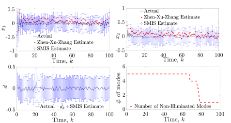
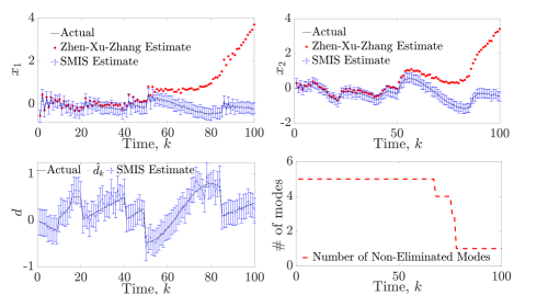
Figure 1: Actual states $x_{1}$, $x_{2}$, and their estimates, as well as the unknown input $d$ and its estimates, and the number of non-eliminated modes at each time step in the bounded unknown input scenario (Scenario I), when applying the observer in [23] (Zhen-Xu-Zhang Estimate) and our proposed observer (SMIS Estimate).

Figure 2: Actual states $x_{1}$, $x_{2}$, and their estimates, as well as the unknown input $d$ and its estimates, and the number of non-eliminated modes at each time step in the unbounded unknown input scenario (Scenario II), when applying the observer in [23] (Zhen-Xu-Zhang Estimate) and our proposed observer (SMIS Estimate).

More interestingly, considering the second scenario, i.e., with unbounded unknown inputs, Figure 2 shows that our set-valued estimates still converge, i.e., our observer remains stable, while the estimates of the approach in [23] exceed the boundaries of the compatible sets of states and inputs of our approach after some time steps and display a divergent behavior (cf. Figure 2).

Table 1: Different modes and their $T^{q}_{2}$ in Scenario I (i.e., with bounded $d_{k}$).

Mode	$T_{2}^{q}$
$q=1$	[0.3629 -0.2179 ]⊤
$q=2$	[0.1191 0.8715 ]⊤
$q=3$	[-0.6468 0.8390 ]⊤
$q=4$	[0.8103 -0.6681 ]⊤
$q=5$	[0.2780 -0.6793 ]⊤

Table 2: Different modes and their $T^{q}_{2}$ in Scenario II (i.e., with unbounded $d_{k}$).

Mode	$T_{2}^{q}$
$q=1$	[0.4730 -0.3280 ]⊤
$q=2$	[0.2202 0.9826 ]⊤
$q=3$	[-0.7579 0.9401 ]⊤
$q=4$	[0.9214 -0.7792 ]⊤
$q=5$	[0.3891 -0.7804 ]⊤

Further, Tables 2 and 2 show the matrix $T^{q}_{2}$ for each mode $q$ for Scenarios I and II, respectively. It can be verified that the second set of sufficient conditions in Theorem 3 holds, i.e., $T^{q}_{2}\neq T^{q^{\prime}}_{2}$ for all $q\neq q^{\prime}$, for both scenarios. Hence, we expect that all false modes are eliminated, i.e., exactly one (true) mode remains, after some large enough time in both scenarios, which is indeed what we observe in Figures 2 and 2, where the number of non-eliminated modes at each time step is shown.

Moreover, for each mode $q$, the signals $\|r^{q}_{k}\|_{2}$, $\|r^{q|*}_{k}\|_{2}$, $\delta^{q,tri}_{r,k}$ and $\delta^{q,inf}_{r,k}$ are depicted in Figures 4 and 4 for Scenarios I and II, respectively. In both scenarios, we observe that $\delta^{q,inf}_{r,k}$ is smaller than $\delta^{q,tri}_{r,k}$ up until approximately 40 time steps, after which $\delta^{q,tri}_{r,k}$ is smaller/tighter. This is one of the main reasons we considered the minimum of both as the threshold in our mode elimination algorithm (also see Remark 1). Furthermore, for all modes, $\delta^{q,tri}_{r,k}$ is eventually convergent while $\delta^{q,inf}_{r,k}$ diverges, as proven in Lemma 3. So, after some large enough time, $\delta^{q,tri}_{r,k}$ can be used as our upper bound threshold, while $\delta^{q,inf}_{r,k}$ becomes ineffective.

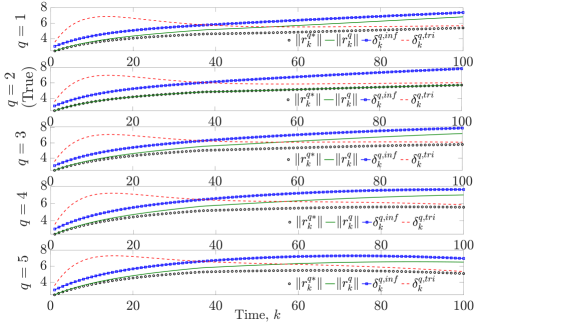
Figure 3: $\|r^{q}_{r,k}\|_{2}$,$\|r^{q|*}_{r,k}\|_{2}$ and their upper bounds for different modes in the bounded unknown input scenario (Scenario I).

Figure 4: $\|r^{q}_{r,k}\|_{2}$,$\|r^{q|*}_{r,k}\|_{2}$ and their upper bounds for different modes in the unbounded unknown input scenario (Scenario II).

6 Conclusion

This paper introduced a novel multiple-model approach for simultaneous mode, unknown input and state estimation for hidden mode switched nonlinear systems with bounded-norm noise and unknown inputs. The proposed approach consists of a bank of mode-matched state and unknown input observer that is optimal in the $\mathcal{H}_{\infty}$ sense and a mode observer, which eliminates inconsistent modes and their corresponding observers at each time step. The proposed mode elimination criterion is based on the use of a provably finite-valued upper bound for the norm of a residual signal as the threshold. Moreover, we provided a tractable approach to compute the threshold signal and proved the convergence of the upper bound /threshold signal as well as derived sufficient conditions for eventually eliminating all false modes when using our mode elimination algorithm. Finally, we demonstrated the effectiveness of our observer using an illustrative example, where we compared our approach with an existing $\mathcal{H}_{\infty}$ observer in the literature under two different scenarios.

References

Appendices

Appendix A System Transformation [11, Appendix A.1]

For $q\in\mathbb{Q}$, let $p_{H^{q}}\triangleq{\rm rk}(H^{q})$. Using singular value decomposition, we rewrite the direct feedthrough matrix $H^{q}$ as $H^{q}=\begin{bmatrix}U^{q}_{1}&U^{q}_{2}\end{bmatrix}\begin{bmatrix}\Sigma^{q}&0\\ 0&0\end{bmatrix}\begin{bmatrix}V_{1}^{q\top}\\ V_{2}^{q\top}\end{bmatrix}$, where $\Sigma^{q}\in\mathbb{R}^{p_{H^{q}}\times p_{H^{q}}}$ is a diagonal matrix of full rank, $U^{q}_{1}\in\mathbb{R}^{l\times p_{H^{q}}}$, $U^{q}_{2}\in\mathbb{R}^{l\times(l-p_{H^{q}})}$, $V^{q}_{1}\in\mathbb{R}^{p\times p_{H^{q}}}$ and $V^{q}_{2}\in\mathbb{R}^{p\times(p-p_{H^{q}})}$, while $U^{q}\triangleq\begin{bmatrix}U^{q}_{1}&U^{q}_{2}\end{bmatrix}$ and $V^{q}\triangleq\begin{bmatrix}V^{q}_{1}&V^{q}_{2}\end{bmatrix}$ are unitary matrices. When there is no direct feedthrough, $\Sigma^{q}$, $U^{q}_{1}$ and $V^{q}_{1}$ are empty matrices, and $U^{q}_{2}$ and $V^{q}_{2}$ are arbitrary unitary matrices, while when $p_{H^{q}}=p=l$, $U^{q}_{2}$ and $V^{q}_{2}$ are empty matrices, and $U^{q}_{1}$ and $\Sigma^{q}$ are identity matrices. Then, we decouple the unknown input into two orthogonal components and since $V^{q}$ is unitary, we obtain:

$$d^{q}_{1,k}=V_{1}^{q\top}d^{q}_{k},\quad d^{q}_{2,k}=V_{2}^{q\top}d^{q}_{k},\quad d^{q}_{k}=V^{q}_{1}d^{q}_{1,k}+V^{q}_{2}d^{q}_{2,k}.$$ (39)

So, we can represent system (3) as:

$$\begin{array}[]{rl}x^{q}_{k+1}&=f^{q}(x_{k})+B^{q}u^{q}_{k}+G^{q}_{1}d^{q}_{1,k}+G^{q}_{2}d^{q}_{2,k}+W^{q}w^{q}_{k},\\ y_{k}&={C}^{q}x_{k}+D^{q}_{k}u^{q}_{k}+H^{q}_{1}d^{q}_{1,k}+v^{q}_{k},\end{array}$$ (42)

where $G^{q}_{1}\triangleq G^{q}V^{q}_{1}$, $G^{q}_{2}\triangleq G^{q}V^{q}_{2}$ and $H^{q}_{1}\triangleq H^{q}V^{q}_{1}=U^{q}_{1}\Sigma^{q}$. Next, the output $y_{k}$ is decoupled using a nonsingular transformation $T^{q}=\begin{bmatrix}T_{1}^{q\top}&T_{2}^{q\top}\end{bmatrix}^{\top}\triangleq U^{q\top}=\begin{bmatrix}U^{q}_{1}&U^{q}_{2}\end{bmatrix}^{\top}$ to obtain $z^{q}_{1,k}\in\mathbb{R}^{p_{H^{q}}}$ and $z^{q}_{2,k}\in\mathbb{R}^{l-p_{H^{q}}}$ given by

$$\begin{array}[]{lll}z^{q}_{1,k}&\triangleq T^{q}_{1}y_{k}=U_{1}^{q\top}y_{k}={C}^{q}_{1}x_{k}+\Sigma^{q}d^{q}_{1,k}+{D}^{q}_{k,1}u^{q}_{k}+{v}^{q}_{1,k},\\ z^{q}_{2,k}&\triangleq T^{q}_{2}y_{k}=U_{2}^{q\top}y_{k}={C}^{q}_{2}x_{k}+{D}^{q}_{k,2}u^{q}_{k}+{v}^{q}_{2,k},\end{array}$$ (45)

where ${C}^{q}_{1}\triangleq U_{1}^{q\top}{C}^{q}$, ${C}^{q}_{2}\triangleq U_{2}^{q\top}{C}^{q}$, ${D}^{q}_{k,1}\triangleq U_{1}^{q\top}{D}^{q}_{k}$, ${D}^{q}_{k,2}\triangleq U_{2}^{q\top}{D}^{q}_{k}$, ${v}^{q}_{1,k}\triangleq U_{1}^{q\top}{v}^{q}_{k}$ and ${v}^{q}_{2,k}\triangleq U_{2}^{q\top}{v}^{q}_{k}$. This transformation is also chosen such that

$$\left\|\begin{bmatrix}{{v}^{q}_{1,k}}^{\top}&{{v}^{q}_{2,k}}^{\top}\end{bmatrix}^{\top}\right\|_{2}=\|U^{q\top}{v}^{q}_{k}\|{\color[rgb]{0,0,0}_{2}}=\|{v}^{q}_{k}\|_{2}.$$

Appendix B Matrices and Parameters in Proposition 1

$$\tilde{Y}^{q}_{1} \triangleq(P-YC^{q}_{2})\Phi^{q},\quad\tilde{Y}^{q}_{2}\triangleq-(P-YC^{q}_{2})\Phi^{q}\Psi^{q},$$

$$\tilde{\mathbf{M}}_{1} \triangleq-{\kappa}I-\breve{Q},\quad\tilde{\mathbf{M}}_{2}\triangleq-{\kappa}{(L_{f}^{q})}^{2}I+(1-\alpha)P-\tilde{\Gamma},\quad\tilde{\mathbf{M}}_{3}\triangleq{\kappa}I,$$

$$\mathcal{N}^{q}_{21} \triangleq\Psi^{q\top}\Phi^{q\top}(PR^{q}-Y\Omega^{q}-C^{q\top}_{2}Y^{\top}R^{q}),$$

$$\mathcal{N}^{q}_{11} \triangleq\rho^{2}I+2R^{q\top}Y\Omega^{q}-R^{q\top}PR^{q}-\Omega^{q\top}(\Gamma+(\varepsilon^{-1}_{1}+\varepsilon^{-1}_{2})I)\Omega^{q},$$

$$\mathcal{N}^{q}_{31} \triangleq\Phi^{q\top}(Y\Omega^{q}+C^{q\top}_{2}Y^{\top}R^{q}-PR^{q}),$$

$$\mathcal{N}^{q}_{33} \triangleq-\varepsilon_{2}\Phi^{q\top}C^{q\top}_{2}C^{q}_{2}\Phi^{q}+I,$$

$$\mathcal{N}^{q}_{22} \triangleq-I+\alpha P-\varepsilon_{1}\Psi^{q\top}\Phi^{q\top}C^{q\top}_{2}C^{q}_{2}\Phi^{q}\Psi^{q}-{L_{f}^{q}}^{2}I,$$

$${\delta}_{\infty}^{x} \triangleq\begin{cases}{{\delta}_{\infty,1}^{x,q}},&\text{if}\ \theta^{q}_{1}<1,\theta^{q}_{2}\geq 1,\\ {{\delta}_{\infty,2}^{x,q}},&\text{if}\ \theta^{q}_{1}\geq 1,\theta^{q}_{2}<1,\\ \min({{\delta}_{\infty,1}^{x,q},{\delta}_{\infty,2}^{q,x}}),&\text{if}\ \theta^{q}_{1}<1,\theta^{q}_{2}<1,\end{cases},$$

$${\delta}_{\infty,1}^{x,q} \triangleq\rho^{\star}_{q}\sqrt{\frac{{\eta^{q}_{w}}^{2}+{\eta^{q}_{v}}^{2}}{{\lambda_{\min}(P^{q})(1-\theta^{q}_{1})}}},$$

$${\delta}_{\infty,2}^{x,q} \triangleq\frac{\overline{\eta}^{q}}{1-\theta^{q}_{2}},$$

$$\theta^{q}_{1} \triangleq{{\textstyle\frac{|\lambda_{\max}(P^{q})-1|}{\lambda_{\min}(P^{q})}}},$$

$${\theta_{2}}^{q} \triangleq(L^{q}_{f}+\|\Psi^{q}\|_{2})\|(I-\tilde{L}^{q}C^{q}_{2})\Phi^{q}\|_{2},$$

$$\overline{\eta}^{q} \triangleq\|\Re^{q}\|_{2}\eta^{q}_{v}+\|\Psi^{q}\Phi^{q}W^{q}\|_{2}\eta^{q}_{w},$$

$$\Omega^{q} \triangleq C^{q}_{2}R^{q}-Q^{q},$$

$${\delta}^{d,q}_{\infty} \triangleq\beta^{q}{\delta}^{x,q}_{\infty}+\overline{\alpha}^{q},$$

$$\Re^{q} \triangleq-(\Psi^{q}\Phi^{q}G^{q}_{1}M^{q}_{1}T^{q}_{1}+\Psi^{q}G^{q}_{2}M^{q}_{2}T^{q}_{2}+\tilde{L}^{q}T^{q}_{2}),$$

$$\beta^{q} \triangleq\|V_{1}^{q}M^{q}_{1}C^{q}_{1}-V^{q}_{2}M^{q}_{2}C^{q}_{2}\Psi^{q}\|_{2}+L^{q}_{f}\|V^{q}_{2}M^{q}_{2}C^{q}_{2}\|_{2},$$

$$\overline{\alpha}^{q} \triangleq\|V^{q}_{2}M^{q}_{2}C^{q}_{2}\|_{2}\eta^{q}_{w}+\big{[}\|(V^{q}_{2}M^{q}_{2}C^{q}_{2}G^{q}_{1}-V^{q}_{1})M^{q}_{1}T^{q}_{1}\|{\color[rgb]{0,0,0}_{2}}+\|V^{q}_{2}M^{q}_{2}T^{q}_{2}\|{\color[rgb]{0,0,0}_{2}}\big{]}\eta^{q}_{v}.$$

References

- [1] R. Verma, D. Del Vecchio, Safety control of hidden mode hybrid systems, IEEE Transactions on Automatic Control 57 (1) (2011) 62–77.
- [2] S. Z. Yong, M. Zhu, E. Frazzoli, Switching and data injection attacks on stochastic cyber-physical systems: Modeling, resilient estimation, and attack mitigation, ACM Transactions on Cyber-Physical Systems 2 (2) (2018) 9.
- [3] S. Z. Yong, M. Zhu, E. Frazzoli, Simultaneous mode, input and state estimation for switched linear stochastic systems, International Journal of Robust and Nonlinear Control 31 (2) (2021) 640–661.
- [4] Y. Bar-Shalom, T. Kirubarajan, X. Li, Estimation with Applications to Tracking and Navigation, John Wiley & Sons, Inc., New York, NY, USA, 2002.
- [5] E. Mazor, A. Averbuch, Y. Bar-Shalom, J. Dayan, Interacting multiple model methods in target tracking: a survey, IEEE Transactions on Aerospace and Electronic Systems 34 (1) (1998) 103–123.
- [6] M. Dahleh, I. Diaz-Bobillo, Control of uncertain systems: a linear programming approach, Prentice-Hall, Inc., 1994.
- [7] J. Shamma, K. Tu, Set-valued observers and optimal disturbance rejection, IEEE Trans. on Automatic Control 44 (2) (1999) 253–264.
- [8] F. Blanchini, M. Sznaier, A convex optimization approach to synthesizing bounded complexity filters, IEEE Transactions on Automatic Control 57 (1) (2012) 216–221.
- [9] S. Z. Yong, Simultaneous input and state set-valued observers with applications to attack-resilient estimation, in: 2018 Annual American Control Conference (ACC), IEEE, 2018, pp. 5167–5174.
- [10] M. Khajenejad, S. Z. Yong, Simultaneous input and state set-valued -observers for linear parameter-varying systems, in: American Control Conference, 2019, pp. 4521–4526.
- [11] M. Khajenejad, S. Z. Yong, Simultaneous state and unknown input set-valued observers for some classes of nonlinear dynamical systems, Submitted to Automatica, Under Review, arXiv preprint arXiv:2001.10125.
- [12] R. Patton, P. Frank, R. Clark, Issues of fault diagnosis for dynamic systems, Springer Science & Business Media, 2013.
- [13] J. Giraldo, D. Urbina, A. Cardenas, J. Valente, M. Faisal, J. Ruths, N. O. Tippenhauer, H. Sandberg, R. Candell, A survey of physics-based attack detection in cyber-physical systems, ACM Computing Surveys (CSUR) 51 (4) (2018) 1–36.
- [14] F. Pasqualetti, F. Dörfler, F. Bullo, Attack detection and identification in cyber-physical systems, IEEE Transactions on Automatic Control 58 (11) (2013) 2715–2729.
- [15] Y. Nakahira, Y. Mo, Attack-resilient , , and state estimator, IEEE Transactions on Automatic Control 63 (12) (2018) 4353–4360.
- [16] J. Kim, C. Lee, H. Shim, Y. Eun, J. Seo, Detection of sensor attack and resilient state estimation for uniformly observable nonlinear systems having redundant sensors, IEEE Transactions on Automatic Control 64 (3) (2018) 1162–1169.
- [17] M. Chong, H. Sandberg, J. Hespanha, A secure state estimation algorithm for nonlinear systems under sensor attacks, in: 2020 59th IEEE Conference on Decision and Control (CDC), IEEE, 2020, pp. 5743–5748.
- [18] M. Khajenejad, S. Z. Yong, Simultaneous mode, input and state set-valued observers with applications to resilient estimation against sparse attacks, in: 2019 IEEE 58th Conference on Decision and Control (CDC), IEEE, 2019, pp. 1544–1550.
- [19] D. Bertsekas, A. Nedic, A. Ozdaglar, Convex analysis and optimization, ser, Athena Scientific optimization and computation series. Athena Scientific.
- [20] H. Bodlaender, P. Gritzmann, V. Klee, J. Van Leeuwen, Computational complexity of norm-maximization, Combinatorica 10 (2) (1990) 203–225.
- [21] R. Rockafellar, Convex analysis, Princeton university press, 2015.
- [22] J. Grcar, A matrix lower bound, Linear Algebra and its Applications 433 (1) (2010) 203–220.
- [23] Q. Zheng, S. Xu, Z. Zhang, Asynchronous non-fragile filtering for discrete-time nonlinear switched systems with quantization, Nonlinear Analysis: Hybrid Systems 37 (2020) 100911.