Distributional data analysis via quantile functions and its application to modelling digital biomarkers of gait in Alzheimer’s Disease

Abstract

With the advent of continuous health monitoring with wearable devices, users now generate their unique streams of continuous data such as minute-level step counts or heartbeats. Summarizing these streams via scalar summaries often ignores the distributional nature of wearable data and almost unavoidably leads to the loss of critical information. We propose to capture the distributional nature of wearable data via user-specific quantile functions (QF) and use these QFs as predictors in scalar-on-quantile-function-regression (SOQFR). As an alternative approach, we also propose to represent QFs via user-specific L-moments, robust rank-based analogs of traditional moments, and use L-moments as predictors in SOQFR (SOQFR-L). These two approaches provide two mutually consistent interpretations: in terms of quantile levels by SOQFR and in terms of L-moments by SOQFR-L. We also demonstrate how to deal with multi-modal distributional data via Joint and Individual Variation Explained (JIVE) using L-moments. The proposed methods are illustrated in a study of association of digital gait biomarkers with cognitive function in Alzheimer’s disease (AD). Our analysis shows that the proposed methods demonstrate higher predictive performance and attain much stronger associations with clinical cognitive scales compared to simple distributional summaries. Wearable data; Quantile functions; L-Moments; Scalar-on-quantile-function regression; JIVE; Alzheimer’s disease; Gait.

1 Introduction

Wearables now generate continuous streams of data that capture minute-level physical activity, heart rhythms and other physiological signals. These streams are a rich source of information and can be used for a deeper understanding of human behaviours and their influence on human health and disease. Common analytical practice in many epidemiological and clinical studies employing wearables is to use simple scalar summaries such as total activity count (TAC), minutes of moderate-to-vigorous-intensity physical activity (MVPA) (Varma and others, 2017; Bakrania and others, 2017) or total step count (TSC) (Reider and others, 2020; Mc Ardle and others, 2020). However, collapsing the entire stream of data into a single metric completely ignores temporal (diurnal or time of the day) and distributional aspects of wearable data.

Temporal aspect of wearable data can be accounted for with functional data analysis (FDA) that treats wearable data streams as functional observations recorded over 24 hours (Morris and others, 2006; Xiao and others, 2015; Goldsmith and others, 2016, 2015). Association between accelerometry-estimated temporal functional profiles and variables of interest such as health outcomes, age, BMI, and others can be studied within FDA using scalar-on-function (SOFR) or function-on-scalar (FOSR) regression (Morris, 2015) models. In addition to diurnal (over 24-hour) modelling, FDA approaches help to model weekly and seasonal variation in accelerometric signal (Huang and others, 2019; Xiao and others, 2015). Co-registration (or warping) is often a desirable pre-processing step to make sure the amplitude and phase variations are properly separated during diurnal modelling (Dryden and Mardia, 2016; Wrobel and others, 2019).

Distributional aspect of wearable data can be captured via modelling user-specific distributions. Augustin and others (2017) proposed to summarize accelerometry activity counts recorded over 24-hours with user-specific histograms. They proposed to use these histograms as predictors in scalar-on-function regression. The main limitations of this approach include i) possibly unequal (effective) support across user-specific histograms, ii) inability to model specific quantiles of the distribution, which, as it will be demonstrated below, could be of a great practical interest, iii) scale-dependence. McKeague and Chang (2019) developed an empirical likelihood based functional ANOVA test for comparing groups of subjects based on their ordered activity profiles to model the amounts of time spent by subjects doing activity above a certain threshold. Compositional data analysis (CoDA) (Aitchison, 1982; Dumuid and others, 2019, 2020) is another group of methods to model continuously measured wearable data. Petersen and Müller (2016) and Hron and others (2016) developed functional compositional methods to analyse samples of densities. Petersen and others (2021) provides a nice accessible tutorial style review of recent developments in that area. Distribution-on-distribution regression models were suggested by Chen and others (2021) and Ghodrati and Panaretos (2021) who used Wasserstein-distances and optimal transport ideas. Additionally, Talská and others (2021) developed a compositional scalar-on-function regression method using a centred logratio transformation (Aitchison, 1982) of subject-specific densities. This has been done by mapping densities from the Bayes space of density functions (Van den Boogaart and others, 2014) to a Hilbert $L^{2}$ space and then performing traditional functional data modelling. Matabuena and others (2021) proposed to use subject-specific densities of glucose measures collected with continuous glucose monitoring (CGM) as predictors (as well as response) and demonstrated advantages of this approach over the use of summary measures typically employed in CGM studies. Specifically, a non-parametric kernel functional regression model was developed that employed a 2-Wasserstein distance to model scalar outcomes and glucodensity predictors.

In this article, we put forward an alternative to the above compositional functional approaches and propose to use subject-specific quantile functions to capture the distributional nature of wearable data. Our approach overcomes the limitations i) and ii) as in (Augustin and others, 2017) and provides a more flexible way to summarize distributional properties of wearable data. Matabuena and Petersen (2021) used a quantile-function representation of NHANES 2003-2006 accelerometry data to predict health outcomes using survey weighted nonparametric regression model that employed a 2-Wasserstein distance. Note that compared to analyzing density functions in a nonlinear space (Talská and others, 2021) or using nonparametric methods based on distances or kernels (Matabuena and Petersen, 2021), our method is semiparametric and offers direct interpretability in terms of the quantile-levels of subject-specific distribution. There is rich literature on quantile functions (Gilchrist, 2000; Powley, 2013) in statistical modelling and decision theoretic analysis. Quantile functions enjoy many mathematical properties, which make them particularly useful for distributional modelling. Quantile representations have been used in symbolic data literature for regression modelling of both quantile functions responses and predictors. The approach is based on the use of $\ell_{2}$ Wasserstein distance (Irpino and Verde, 2013; Verde and Irpino, 2010). Zhang and Müller (2011) proposed a method for density function estimation using a quantile synchronization approach, instead of using the cross-sectional average density which does not incorporate time-warping. Recently, Yang and others (2020) proposed quantile-function-on-scalar regression approaches for modelling quantile functions as outcomes. Having quantile functions as outcomes imposes constraints on the regression that requires a regression approximant to be a valid quantile function Yang (2020). In our regression applications, we do not have these constraints because user-specific quantile functions are used as functional predictors.

As a motivating study, we will focus on continuous accelerometry data collected over one week in a sample of $86$ community-dwelling older adults with mild Alzheimer’s disease (AD) and cognitively normal controls (CNC)(Varma and Watts, 2017; Varma and others, 2021). AD is the most common form of dementia and cases are projected to more than double in the next 40 years (Alzheimer’s Association, 2020; Hebert and others, 2013) in the United States. The absence of any permanent treatment to cure AD makes early detection of cognitive impairment paramount. Digital biomarkers have recently been considered for early detection of AD as an alternative to more invasive and expensive fluid and imaging markers (Kourtis and others, 2019). Specifically, digital biomarkers that reflect alterations in gait may help to predict AD due to the close relationship between complex cognitive functions and gait (Yogev-Seligmann and others, 2008; Mc Ardle and others, 2019; Varma and others, 2021). In our study, subjects wore an accelerometer on their hip in order to measure continuous, community activity over 7 days. Using a validated processing pipeline (Weiss and others, 2014), we measured 52, domain-specific gait parameters during identified episodes of sustained walking (defined as walking longer than 60 seconds) over the course of the 7-day data collection period.

Figure 1 shows the user-specific quantile functions of accelerometry-estimated step velocity for mild-AD and CNC group. Interestingly, for each group, the average quantile function is directly related to the Wasserstein barycenter of their respective distribution (Bigot and others, 2018). The average quantile functions, therefore, can be highly informative and can identify parts of the distribution that are most discriminative between groups of interest. The largest difference between the two groups can be seen in the upper quantiles of step velocity. This supports the point that quantile functions can be useful for distributional representations.

Three main methodological contributions of this article are as follows. First, we propose to capture the distributional aspect of wearable data via user-specific quantile functions and use them as predictors in scalar-on-quantile-function regression (SOQFR). This allows us to apply inferential tools of functional data analysis to make inference about the specific quantile levels of distributional predictors. This approach is further generalized using functional generalized additive model (McLean and others, 2014) which can capture possible nonlinear effects of the quantile functions. Such models have strong mathematical interpretations as linear functional of quantile functions or its transformation is known to encode several important characteristics of a continuous distribution (Powley, 2013). Second, we propose to use L-moments to represent user-specific quantile functions via functional decompositions that also preserve distributional information and encode this information via moments. L-moments introduced in Hosking (1990) are robust rank based analogs of traditional moments and they fully define the distribution. We show that SOQFR model can be reduced to a generalized linear model with L-moments (SOQFR-L). These two approaches provide two mutually consistent interpretations: in terms of quantile levels by SOQFR and in terms of L-moments by SOQFR-L. Third, in our motivating application, there are multiple digital biomarkers that can be grouped into five gait domains including Amplitude, Pace, Rhythm, Symmetry, and Variability. Thus, this gives rise to a design with multi-modal distributional data. We demonstrate how L-moments can be used for analyzing joint and individual sources of variation using JIVE (Joint and Individual Variation Explained) (Lock and others, 2013) method.

The rest of this article is organized as follows. In Section 2, we present our modelling framework, introduce the mathematical background for quantile functions, and illustrate the proposed SOQFR approach. In Section 3, we introduce L-moments for distributional data and show how they can be used for SOQFR-L and JIVE. In Section 4, we demonstrate the applications of the proposed methods in the Alzheimer’s disease (AD) study. Section 5 concludes with a discussion on the main contribution and some possible extensions of this work.

2 MODELLING FRAMEWORK

Suppose, we have multiple repeated observations of a variable $X$ per subject denoted by $X_{ij}\hskip 2.84526pt(j=1,\ldots,n_{i})$, for subject $i=1,\ldots,n$, where $n_{i}$ (the number of observations for subject $i$) is typically quite large (e.g., on an average around 100 walking bouts in our study). In some applications (e.g. activity data), $X_{ij}=X_{i}(t_{ij})$ can be observed across various time-points $t_{ij}$. Assume $X_{ij}$ $(j=1,\ldots,n_{i})\sim F_{i}(x)$, a subject-specific cumulative distribution function (cdf), where $F_{i}(x)=P(X_{ik}\leq x)$. Then, we can define subject-specific quantile function $Q_{i}(p)=\inf\{x:F_{i}(x)\geq p\}$. The quantile function completely characterizes the distribution of the individual observations. In this article, we restrict our attention to cases, where both $F_{i}(x)$ s and $Q_{i}(p)$ are continuous, which ensures $Q_{i}=F_{i}^{-1}$, so $F_{i}(Q_{i}(p))=p,\hskip 5.69054ptQ_{i}(F_{i}(x))=x$. This also ensures both quantile function and cdf are strictly increasing in their respective domains (Powley, 2013). Using $X_{ij}$ ($j=1,\ldots,J$) one can calculate $\hat{F}_{i}(x)$, the empirical cdf and then obtain the empirical quantile function $\hat{Q}_{i}(p)=\hat{F}_{i}^{-1}(p)$ ($p\in[0,1]$, the percentile resolution can be determined based on the amount of available data). Estimation of quantile functions can be done via a linear interpolation of order statistics (Parzen, 2004) and does not require a bandwidth selection as in kernel density estimation. In particular, we use the following estimator of quantile functions,

$$\hat{Q}(p)=(1-w)X_{([(n+1)p])}+wX_{([(n+1)p]+1)},$$

where $X_{(1)}\leq X_{(2)}\leq\ldots,X_{(n)}$ are the corresponding order statistics from a sample $(X_{1},X_{2},\ldots,X_{n})$ and $w$ is a weight satisfying $(n+1)p=[(n+1)p]+w$. Quantile functions have a few nice mathematical properties (Gilchrist, 2000; Powley, 2013) that make them particularly suitable for distributional modelling. For convenience, we list some of these properties below.

• A non-negative linear combination of finite number of quantile functions is a quantile function.

• For a probability distribution defined via a quantile function $Q(\cdot)$, all integer moments can be represented as $E(X^{m})=\int_{0}^{1}Q^{m}(p)dp$ (assuming that all moments exist).

• The quantile density function and the $p$-probability density function are defined as $q(p)=Q^{{}^{\prime}}(p)$ and $f(Q(p))$, respectively. Here, $f$ is the density function corresponding to $F$.

• The average of subject-specific quantile functions $\bar{Q}(p)=\frac{1}{n}\sum_{i=1}^{n}Q_{i}(p)$ can be mapped to the Wasserstein barycenter of the measures induced by the respective distributions (Bigot and others, 2018).

• In $L_{2}\hskip 2.84526pt[0,1]$, a distance between any two quantile functions can be defined via the 2-Wasserstein distance $W_{2}$, $d_{2}(F_{1},F_{2})=(\int_{0}^{1}(Q_{1}(p)-Q_{2}(p))^{2}dp)^{1/2}$.

Expansions of quantile functions via orthogonal polynomials are directly related to the components of the Shapiro–Francia Statistic (Takemura, 1983) and L-moments (Hosking, 1990) which will be discussed in greater details in Section 3.

Next section illustrates the use of quantile functions as functional objects in scalar-on-function regression models.

2.1 Scalar-on-quantile-function regression

In this section, we assume that $Y_{i},i=1,\ldots,n$, is an outcome of interest that can be continuous or discrete, coming from an exponential family. We consider the following generalized scalar-on-function regression (SOFR) with quantile functions as predictors which we will refer to as a scalar-on-quantile-function regression (SOQFR) model:

$$E(Y_{i}|X_{i1},X_{i2},\ldots,X_{in_{i}})=\mu_{i},\hskip 5.69054ptg(\mu_{i})=\alpha+\mathbf{Z}_{i}^{T}\bm{\gamma}+\int_{0}^{1}Q_{i}(p)\beta(p)dp.$$ (1)

Here $g$ is a known link function, $Z_{i}$ are confounding scalar covariates and $Q_{i}(p)$’s ($i=1,2,\ldots,n$) are the subject-specific quantile functions of predictor of interest $X_{ij}$. The smooth coefficient function $\beta(p)$ represents the functional effect of the quantile function at quantile level $p$. As pointed out in Reiss and others (2017), locations with largest $|\beta(p)|$ are the most influential to the response and of practical interest. In the special case of $\beta(p)=\beta$, model (1) reduces to a usual GLM on the mean ($\nu_{i}=\int_{0}^{1}Q_{i}(p)dp$) of X (the variable on which we have multiple observations)

$$g(\mu_{i})=\alpha+\mathbf{Z}_{i}^{T}\bm{\gamma}+\beta\int_{0}^{1}Q_{i}(p)dp=\alpha+\mathbf{Z}_{i}^{T}\bm{\gamma}+\beta\nu_{i}.$$ (2)

Several methods exist in the literature for estimation of the smooth coefficient function $\beta(p)$ (Goldsmith and others, 2011; Marx and Eilers, 1999) in SOFR. In this article, we follow a smoothing spline estimation method. The penalized negative log likelihood criterion for estimation is given by

$$R(\alpha,\bm{\gamma},\beta(\cdot))=-2logL(\alpha,\bm{\gamma},\beta(\cdot);Y_{i},\mathbf{Z}_{i}^{T},Q_{i}(p))+\lambda\int_{0}^{1}\{\beta^{{}^{\prime\prime}}(p)\}^{2}dp.$$ (3)

The second derivative penalty on $\beta(p)$ ensures the resulting coefficient function is smooth. We model the unknown coefficient functions $\beta(p)$ using univariate basis function expansion as $\beta(p)=\sum_{k=1}^{K}\beta_{k}\theta_{k}(p)=\bm{\theta}(p)^{T}\bm{\beta}$, where $\bm{\theta}(p)=[\theta_{1}(p),\theta_{2}(p),\ldots,\theta_{K}(p)]^{T}$ and $\bm{\beta}=(\beta_{1},\beta_{2},\ldots,\beta_{K})^{T}$ is the vector of unknown coefficients. In this article, we use cubic B-spline basis functions, however, other basis functions can be used as well. The linear functional effect then becomes $\int_{0}^{1}Q_{i}(p)\beta(p)dp=\sum_{k=1}^{K}\beta_{k}\int_{0}^{1}Q_{i}(p)\theta_{k}(p)dp=\sum_{k=1}^{K}\beta_{k}Q_{ik}=\mathbf{Q}_{i}^{T}\bm{\theta}$. The minimization criterion in (3) now can be reformulated as,

$$R(\psi)=R(\alpha,\bm{\gamma},\bm{\beta})=-2logL(\alpha,\bm{\gamma},\bm{\beta};Y_{i},\mathbf{Z}_{i},\mathbf{Q}_{i})+\lambda\bm{\beta}^{T}\amsmathbb{P}\bm{\beta},$$ (4)

where $\amsmathbb{P}$ is the penalty matrix given by $\amsmathbb{P}=\{\int_{0}^{1}\bm{\theta}^{{}^{\prime\prime}}(p)\bm{\theta}^{{}^{\prime\prime}}(p)^{T}dp\}$. This minimization can be carried out using the Newton-Raphson algorithm implemented under generalized additive models (GAM) (Wood and others, 2016; Wood, 2017). The smoothing parameter $\lambda$ can be chosen using REML, information criteria like AIC, BIC, or data driven methods such as Generalized CV. We use the refund package (Goldsmith and others, 2018) in R (R Core Team, 2018) for implementation of SOFR.

2.2 Functional Generalized Additive Regression with Quantile Functions

The SOQFR model (1) assumes a linear association between the quantile function and the outcome. SOQFR model can be extended to functional generalized additive model (FGAM) of McLean and others (2014) which can be used to capture nonlinear effects of quantile function $Q(p)$. We denote this model as FGAM-QF. Specifically, we model the link function $g(\cdot)$ as

$$g(\mu_{i})=\alpha+\mathbf{Z}_{i}^{T}\bm{\gamma}+\int_{0}^{1}F(Q_{i}(p),p)dp.$$ (5)

The bivariate function $F\{Q(p),p\}$ is smooth function on $\mathbb{R}\times[0,1]$, capturing effect of the subject-specific quantile function $Q(p)$ at quantile level $p$. In a special case of $F\{Q(p),p\}=Q(p)\beta(p)$, FGAM-QF reduces to model (1). The estimation procedure for FGAM-QF is discussed in Appendix 1 of Supplementary Material. It can be shown that the FGAM-QF is flexible and remains invariant under any continuous transformation of predictors (McLean and others, 2014).

3 L-moments

L-moments were introduced and popularized by Hosking (1990). If $X_{1},X_{2},\ldots,X_{n}$ are $n$ independent copies of $X$ and $X_{1:n}\leq X_{2:n}\leq\ldots\leq X_{n:n}$ are their corresponding order statistics, then the $r$-order L-moment is defined as follows

$$L_{r}=r^{-1}\sum_{k=0}^{r-1}(-1)^{k}{r-1\choose k}E(X_{r-k:r})\hskip 8.53581ptr=1,2,\ldots$$ (6)

The first order L-moment, $L_{1}=EX_{1:1}=EX$, so it just coincides with the traditional first moment of $X$. The second order L-moment, $L_{2}=1/2(E(X_{2:2})-E(X_{1:2}))$, equals exactly a half of mean absolute difference (Gini-coefficient) and can be seen as a robust measure of scale. The third and fourth order L-moments, $L_{3}=1/3E(X_{3:3}-2X_{2:3}+X_{1:3})$ and $L_{4}=1/4E(X_{4:4}-3X_{3:4}+3X_{2:4}-X_{1:4})$, capture higher-order distributional properties and normalized by $L_{2}$ can be interpreted as robust counterparts of traditional higher-order moments such as skewness and kurtosis. Sample L-moments can be calculated using corresponding U-statistics. There are three main advantages of L-moments over traditional moments. First, all L-moments exist as long as $E(X)<\infty$. Second, L-moments are unique and fully define the distribution. Third, L-moments are defined via linear combinations of order statistics, and are typically more robust compared to the traditional moments.

In our approach, we leverage an alternative representation of L-moments as projections of quantile functions on shifted Legendre polynomial basis. Specifically, L-moments of order $r$ can be represented as

$$L_{r}=\int_{0}^{1}Q(p)P_{r-1}(p)dp,$$ (7)

where $P_{r}(p)$ is the shifted Legendre polynomials (LP) of degree $r$ defined as follows

$$P_{r}(p)=\sum_{k=0}^{r}s_{r,k}p^{r},\quad s_{r,k}=(-1)^{r-k}{r\choose k}{r+k\choose k}=\frac{(-1)^{r-k}(r+k)!}{(k!)^{2}(r-k)!}.$$ (8)

Shifted Legendre polynomials have standard orthogonality properties on $[0,1]$ as

$$\int_{0}^{1}P_{s}(p)P_{r}(p)dp=\delta_{rs}(\frac{1}{2r+1}),$$ (9)

where $\delta_{rs}=I(r=s)$. Thus, quantile function $Q(p)$ has the following decomposition

$$Q_{k}(p)=\sum_{r=1}^{k}(2r-1)P_{r-1}(p)\int_{0}^{1}Q(p)P_{r-1}(p)dp=\sum_{r=1}^{k}(2r-1)L_{r}P_{r-1}(p)\to Q(p),k\to\infty.$$ (10)

Note that this approximation can be poor in the tails, if the distribution is heavy tailed (Hosking, 1990). For a non negative random variable $X$, regular moments can be expressed as $\mu_{k}=EX^{k}=\mu_{k}(\bar{F})=k\int_{0}^{\infty}x^{k-1}\bar{F}(x)dx=\mu_{k}(Q)=\int_{0}^{1}Q^{k}(p)dp$, where $\bar{F}(x)=1-F(x)$, and $F(x)$ is the cumulative distribution function for $X$.

Representation of L-moments via Legendre polynomial basis helps to see a geometrical intuition behind the existence of all L-moments, given a finite mean. Supplementary Figure S1 shows a comparison between $\mu_{k}(\bar{F})$, $\mu_{k}(Q)$ and $L_{k}(Q)=\int_{0}^{1}Q(p)P_{k-1}(p)dp$ for a log-normal and a Beta distribution. Note that for the integral $\mu_{k}(\bar{F})$, $kx^{k-1}\bar{F}(x)$ can diverge over $x$. Similarly, for the integral $\mu_{k}(Q)$, $Q^{k}(p)$ can diverge over $p$. However, functions $Q(p)P_{k-1}(p)$ always lie between $Q(p)$ and $-Q(p)$, which guarantees the existence of all L-moments as long as $\int_{0}^{1}Q(p)dp<\infty$.

3.1 Scalar-on-quantile-function regression (SOQFR) using L-moments

In this section, we develop a scalar-on-quantile-function regression method using subject-specific L-moments (SOQFR-L). The SOQFR-L approach will provide the interpretation of SOQFR results in terms of the regression coefficients for L-moments. Since the shifted Legendre polynomials form an orthogonal basis of $L_{2}[0,1]$, we can approximate $\beta(p)$ in model (1) in terms of a truncated basis expansion as $\beta(p)=\sum_{k=1}^{K}\beta_{k}P_{k-1}(p)$. Thus, the SOQFR model (1) reduces to a standard GLM on the subject-specific L-moments as

$$g(\mu_{i})=\alpha+\mathbf{Z}_{i}^{T}\bm{\gamma}+\sum_{k=1}^{K}\beta_{k}\int_{0}^{1}Q_{i}(p)P_{k-1}(p)dp=\alpha+\mathbf{Z}_{i}^{T}\bm{\gamma}+\sum_{k=1}^{K}\beta_{k}L_{ik}.$$ (11)

The unknown basis coefficients $\beta_{k}$ in this SOQFR-L representation capture a linear effect of the L-moments of the subject-specific distribution. Note that the first order L-moment, $L_{1}$, equals mean of the subject-specific distribution, therefore, model (11) is more general than using the subject-specific mean.

SOQFR-L approach can be seen as somewhat analogous to functional principal component regression (fPCR) method (Reiss and others, 2017), where fPC scores are used for supervised learning. L-moments are projections on orthogonal basis functions, and hence, can be interpreted in similar additive manner while additionally providing moment-based characterization of underlying distributions. Thus, the proposed approach allows mutually consistent interpretation of the results from the quantile-level perspective from SOQFR via $\beta(p)$ and from the L-moment level perspective (robust distributional summaries) from SOQFR-L via $\beta_{k}$’s.

The number of L-moments $K$ to be retained (the number of basis functions for modelling $\beta(p)$) can be treated as a tuning parameter and can be chosen in a data-driven way using cross-validation, proportion of variance explained or information criteria such as AIC or BIC. The proportion of variance explained (PVE) by the first $k$ ($k=2,3\ldots,$) L-moments of the subject specific quantile function $Q_{i}(p)$ can be defined as

$$\tau_{k}^{2}=1-\frac{\int_{0}^{1}(Q_{i}(p)-Q_{i}^{k}(p))^{2}dp}{\int_{0}^{1}(Q_{i}(p)-\mu_{i})^{2}dp},$$

where $Q_{i}^{k}(p)$ is the approximate quantile function based on first $k$ L-moments as in equation (10). Note that, $Q_{i}^{1}(p)=L_{i1}=\mu_{i}$, hence $\tau_{1}^{2}=0$ and $\tau_{k}^{2}(k\geq 2)$ represents the amount of variance in the subject specific quantile function explained by the first k subject-specific L-moments. In the applications of this article, we restrict our attention to the first 4 L-moments ($K=4$) to retain the interpretability of the models in terms of the first 4 distributional summaries (similar to the first 4 traditional moments typically used in most of applications).

Nonlinear associations can be modelled using nonlinear extensions of SOFR (Reiss and others, 2017) that can be seen as a functional analogue of the single index model(Stoker, 1986). In particular, we can use this model

$$E(Y_{i}|X_{i1},X_{i2},\ldots,X_{iJ})=\mu_{i},\qquad g(\mu_{i})=\alpha+\mathbf{Z}_{i}^{T}\bm{\gamma}+h\left(\int_{0}^{1}Q_{i}(p)\beta(p)dp\right),$$ (12)

where $h(\cdot)$ is a smooth unknown function on real line. Expanding $\beta(p)$ via Legendre polynomial basis, we get a traditional single index model where the L-moments play a role of predictors as $g(\mu_{i})=\alpha+\mathbf{Z}_{i}^{T}\bm{\gamma}+h(\mathbf{L}_{i}^{T}\bm{\beta})$. Traditional estimation methods for the single index model (Wang and Yang, 2009; Ichimura, 1991) can be applied to estimate both $h(\cdot)$ and $\bm{\beta}$. Another alternative way to capture nonlinear association between the outcome and quantile functional predictors is to use a generalized additive model (GAM) with L-moments as $g(\mu_{i})=\alpha+\mathbf{Z}_{i}^{T}\bm{\gamma}+\sum_{k=1}^{K}h_{k}(L_{ik}).$ The GAM approach using L-moments is analogous to the “functional additive model” of Müller and Yao (2008), where fPC scores were used for scalar-on-function modelling and offers additional interpretability in terms of nonlinear effects of robust distributional summaries of data.

3.2 Modelling multi-modal distributional data via Joint and Individual Variation Explained and L-moments

In this section, we demonstrate how L-moments can be used to identify joint and individual sources of variation in multi-modal distributional data. Suppose, we have repeated measures data from multiple domains $d=1,2,\ldots,D$ each consisting of $R_{d}$ different features on the same subjects $i=1,2,\ldots,n$. Thus, we have subject-specific quantile functions $Q_{i}^{(d,r_{d})}(p)$ for $r_{d}$-th feature within domain $d$ ($r_{d}=1,2,\ldots,R_{d}$). In many applications, it is important to identify joint and individual sources of variation in these multi-modal distributional data. For scalar data, Lock and others (2013) introduced joint and individual variation explained (JIVE) for integrative analysis of data coming from multiple domains. JIVE decomposes the original block data matrix into three parts, a low rank approximation capturing the joint structure and low rank approximations capturing domain-specific individual variation and noise. For multi-modal distributional data $Q_{i}^{(d,r_{d})}(p)$, we propose to use L-moments to analyze joint and individual sources of variation. Specifically, let $L_{ik}^{(d,r_{d})}=\int_{0}^{1}Q_{i}^{(d,r_{d})}(p)P_{k-1}(p)$ be the $k$-th L-moment ($k=1,2,\ldots,K$) for $Q_{i}^{(d,r_{d})}$. For each feature, we form the vector of L-moments and denoting it as $\mathbf{L}_{i}^{(d,r_{d})}$. Then, for each domain $d$, we get the following vector of L-moments $\mathbf{L}_{i}^{(d)}=[\mathbf{L}_{i}^{(d,1)^{T}},\mathbf{L}_{i}^{(d,2)^{T}},\ldots,\mathbf{L}_{i}^{(d,R_{d})^{T}}]^{T}$, where $\mathbf{L}_{i}^{(d)}$ is a $v_{d}=KR_{d}-$dimensional vector consisting of all L-moments for all features in domain $d$. Next, we apply JIVE decomposition of these L-moments vectors as $\mathbf{L}_{i}^{(d)}=\mathbf{J}_{i}^{d}+\mathbf{A}_{i}^{d}+\bm{\varepsilon}_{i}^{d}=\mathbb{\Phi}_{J}^{d}\bm{\xi}_{J,i}+\mathbb{\Phi}_{A}^{d}\bm{\xi}_{A,i}^{d}+\bm{\varepsilon}_{i}^{d}$. Here, $\mathbf{J}_{i}^{d}$ and $\mathbf{A}_{i}^{d}$ represent the low rank joint and individual structures with rank $s$ and $s_{d}$, respectively, and $\bm{\varepsilon}_{i}^{d}$ is the residual noise. Matrices of loadings for joint and individual structures are given by $\mathbb{\Phi}_{J}^{d}\in\amsmathbb{R}^{\nu_{d}\times S}$, $\mathbb{\Phi}_{A}^{d}\in\amsmathbb{R}^{\nu_{d}\times S_{d}}$, and $\bm{\xi}_{J,i}$, $\bm{\xi}_{A,i}^{d}$ are corresponding joint and individual scores for subject $i$. The summary of the proposed JIVE approach is presented as an Algorithm in Appendix 2 of Supplementary Material. The ranks $s$, $s_{d}$ can be chosen using BIC or permutation tests (Lock and others, 2013). The number of L-moments $K$ can be chosen beforehand in a data-driven way. The joint and individual scores $\bm{\xi}_{J,i}$, $\bm{\xi}_{A,i}^{d}$ can further be used for supervised learning purposes. We use the r.jive package (O’Connell and Lock, 2017) in R (R Core Team, 2018) for implementation of JIVE.

4 DIGITAL GAIT BIOMARKERS IN ALZHEIMERS’ DISEASE

Accelerometry data for this study (Varma and others, 2021) were collected using a GT3x+ tri-axial accelerometer in a sample of $86$ older participants including $38$ mild-AD and $48$ age-matched cognitively normal controls (CNC). Descriptive statistics on several baseline variables including age, sex, BMI, years of education, VO₂ max (maximum rate of oxygen consumption during a treadmill test) for the whole sample, and mild-AD and CNC groups are reported in Table S1 of Supplementary Material. Briefly, the sample had $50\%$ female and average age of 73.2 years. There were no statistical differences between mild-AD and CNC group were found across age, BMI, and VO₂ max. Compared to CNC group, mild-AD group had a significantly smaller percentage of females (26.3 vs 68.7) and lower education (15.6 years vs 17.4 years).

The accelerometer was placed on the dominant hip of the participants via elastic belt. Activity was monitored continuously for seven days and, subsequently, gait parameters were obtained using a processing pipeline developed and validated in the Parkinson’s Disease (PD) field (Weiss and others, 2014). The pipeline outputs 52 gait metrics coming from 5 gait domains of Amplitude (8 metrics), Pace (3 metrics), Rhythm (13 metrics), Symmetry (9 metrics), and Variability (19 metrics). The complete list of gait metrics, along with their description and associated domains have been described in Varma and others (2021) and is given in Table S4 of Supplementary Material. Each gait metric is calculated every time a subject completes a sustained bout of walking of at least 60 sec; this provides multiple observations per subject across each of the seven wear days. Figure 1 reveals distributional nature of this data for a particular gait metric “step velocity” for AD and CNC group.

4.1 Discrimination of AD using SOQFR

One of the primary objectives of our analysis is to explore how well the distributional representation of digital gait biomarkers can discriminate between mild-AD and CNC. To do that, we perform SOQFR and FGAM-QF with logit-link to model mild-AD vs CNC. We fit multiple models using each gait metrics separately and adjust for age and sex. For evaluation of the models, we use the “deviance explained” criterion in GAM (Wood, 2017), which represents the proportion of null deviance explained by the respective models. We also report the average cross-validated area under the curve (AUC) of the receiver operating characteristic as an estimate for the out-of-sample prediction performance of the considered models. In particular, we perform a repeated 10-fold cross-validation (B=100 times) and report the average cross-validated AUC (cvAUC).

We use the refund (Goldsmith and others, 2018) package within R (R Core Team, 2018) for implementation of SOQFR and FGAM-QF. Table Distributional data analysis via quantile functions and its application to modelling digital biomarkers of gait in Alzheimer’s Disease displays the top ten gait metrics ranked by the proportion of deviance explained in SQOFR and FGAM-QF. The variables in FGAM-QF consistently explain higher deviance which is expected. Particularly interesting are “Mean_Stride_Time__s_” (mean stride time) and “Mean_Step_Time_s_” (mean step time). Used within FGAM-QF, they explain a much higher proportion of deviance ($0.63$) compared to SOQFR ($0.37$). This might be due to possible nonlinear effects of the quantile functions for these variables. The metrics “Step_Velocity__cm_sec_” (step velocity), “Distance__m_” (distance), “Cadence_V_time_domain_” (cadence) perform more or less similarly using either SOQFR or FGAM-QF, indicating a linear effect. The average cvAUCs from SOQFR and FGAM-QF models illustrate an improved predictive performance compared to generalized linear models with the mean of the gait metrics (adjusted for age and sex), specifically for the measures of step velocity, cadence, distance, and mean stride time.

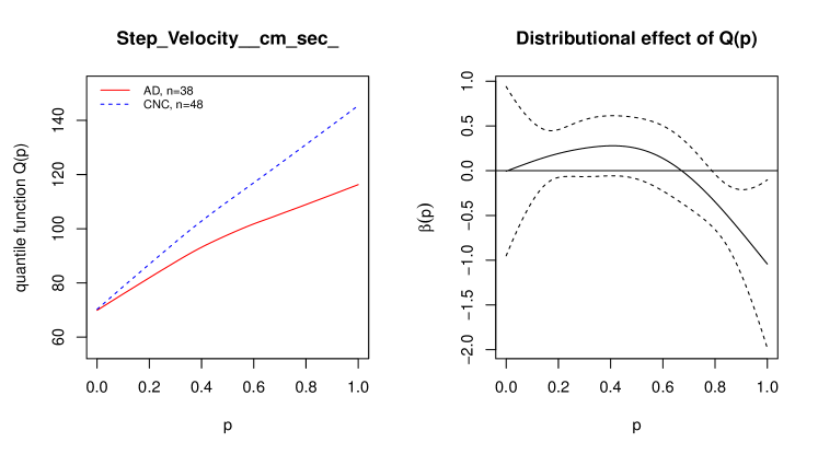
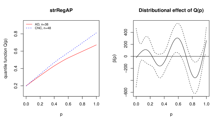
Figure 2: Estimated linear functional effects $\beta(p)$ of quantile functions of step velocity (top right) and stride regularity (bottom right). The average quantile functions of the gait features for the AD (solid lines) and CNC group (dashed lines) are shown in the left column.

Figure 2 displays the estimated functional effects for the top 2 metrics for SOQFR, “strRegAP” (stride regularity) and step velocity, along with their average quantile functions. The 95$\%$ pointwise confidence intervals (Goldsmith and others, 2011) for the estimated functional effects are also shown. We see a clear negative effect in the upper quantiles for both step velocity and stride regularity, indicating higher the maximal performance for these measures lower the odds of AD, which is very interesting from a clinical perspective. The additive quantile functional effects of the metrics mean stride time and step velocity obtained using FGAM-QF are displayed in Figure S2 of Supplementary Material along with the average quantile functions of AD and CNC groups. The sliced effect of the corresponding surfaces are shown in Supplementary Figure S3. For mean stride time, both tails can be informative. Interestingly, a higher maximal or minimal performance of this metric seems to be associated with higher odds of AD. There is a visible non-linearity in the upper tail of the estimated bivariate surface and the sliced effect $\hat{F}(q,p)$. FGAM-QF captures this non-linearity and therefore produces a superior performance for this metric in terms of deviance explained ($63\%$) compared to the SOQFR model ($37\%$). The estimated bivariate surface of the quantile effect is more or less linear for step velocity and is highly negative in the upper tail (evident from the sliced effect). Hence high maximal performance in this metric is associated with lower odds of AD. Since the effect of the quantile function for this metric is linear, the performance and inference from FGAM-QF are similar to what we obtain from SOQFR.

4.2 Comparison of SOQFR with histogram based modelling

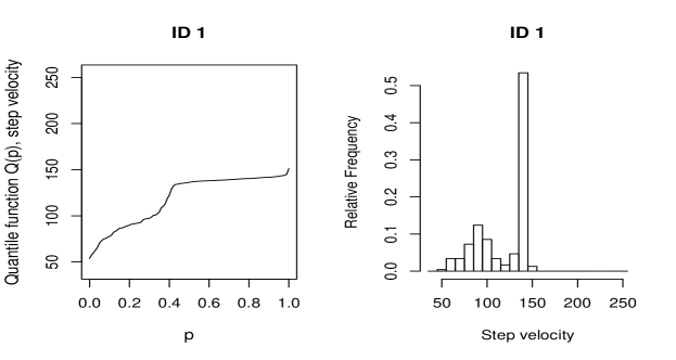
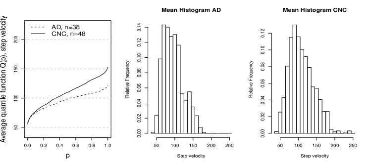
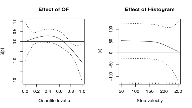
Figure 3: Top panel: the subject-specific quantile function and histogram (relative frequency) of step velocity for subject ID=1. Middle panel: the group means of quantile functions (left) and histograms (right) of step velocity for AD and CNC groups. Bottom panel: estimated functional effect $\beta(p)$ for quantile functions of step velocity (left) and estimated effect $f(x)$ of subject-specific histogram (right).

We compare the proposed SOQFR method with the histogram-based approach by Augustin and others (2017). In particular, we focus on step velocity and obtain subject-specific histograms (relative frequency) in 22 bins of equal width (10) between step velocity values of 35 and 255 (cm/second). Top panel of Figure 3 shows both the quantile function and histogram of step velocity for a random subject from our study. The group average of quantile functions and the group average of histogram (relative frequency) for AD and CNC groups are shown in the middle panel. It is worth noting that the average of quantile functions is a barycenter and is well-defined in terms of 2-Wassterstein distince (Panaretos and Zemel, 2020), while the average of histograms is based on Euclidean distance, not well-defined and included here for illustrative purposes. Visually, the mean histograms are not directly interpretable compared to the averages of quantile functions, which nicely captures the divergence between the two groups in terms of maximal levels of step velocity. Following Augustin and others (2017), we fit a GLM model for the binary outcome of cognitive status (mild-AD vs CNC) with subject-specific histograms $H_{i}(x_{j})$ of step velocity as functional predictors and adjust the model for age and sex. Specifically, the model is as follows: $g(\mu_{i})=\alpha+\mathbf{Z}_{i}^{T}\bm{\gamma}+\sum_{j}H_{i}(x_{j})f_{x}(x_{j}).$ Here $H_{i}(x_{j})$ is the subject-specific histogram (relative frequency) of step-velocity of subject $i$ with some given number at mid-point $x_{j}$ and $f_{x}(x_{j})$ captures the smooth effect of the subject-specific relative frequency at $x_{j}$. We compare the estimates and the performance of this model to the SOQFR model for step velocity. The proportion of deviance explained of the above histogram-based model is $0.30$ compared to $0.50$ for SOQFR. This illustrates higher explanatory power of the subject-specific quantile function $Q_{i}(p)$ compared to the histogram-based representation of step velocity. The estimated smooth effect $f_{x}(x)$ and linear functional effect $\beta(p)$ of step velocity from SOQFR is shown in the bottom panel of Figure 3. The $95\%$ credible intervals from GAM for $f_{x}(x)$ (Wood, 2017) include zero at all values of step velocity and hence subject specific representation of step-velocity in terms of histogram (relative frequency) is not statistically significant. On the contrary, the functional regression coefficient $\beta(p)$ for SOQFR is statistically significant for quantile levels of $p>0.8$. This illustrates that a higher maximal level of step velocity is associated with a reduced odds of AD. Further, we compare the predictive performance of the two approaches in terms of cross-validated area under the curve (AUC) of the receiver operating characteristic. Specifically, we perform a repeated 10-fold cross-validation (B=100 times) and report the average cross-validated AUC (cvAUC). cvAUC of the proposed SOQFR method is calculated to be $0.89$, which is much higher than cvAUC of $0.79$ for the histogram-based approach. This illustrates a higher predictive (discriminatory) power of the quantile function distributional representation of step-velocity in our application.

4.3 Discrimination of AD using SOQFR-L and comparison with SOQFR

In this section, we apply SOQFR-L to stride regularity, step velocity, and cadence, top-performing metrics in SOQFR. Supplementary Figure S4 shows PVE in subject-specific quantile functions of stride regularity, step velocity, and cadence. We observe that the first four L-moments, on average, explain around $92-95\%$ of the variance in those three gait measures. Compared to the traditional or central moments, L-moments are orthogonal projections on the shifted Legendre polynomials, hence they tend to encode less correlated distributional properties. Supplementary Figure S5 shows the heatmap of correlations among the first four L-moments, traditional moments and central moments for cadence. As can be noticed, the traditional and central moments are highly positively correlated among themselves, which is not the case for L-moments.

We fit three separate logit-link SOQFR-L models for each of the three gait metrics. The results are reported in Table 2. Importantly, it is not the mean (equal to $L_{1}$), but the second-order ($L_{2}$) or third-order ($L_{3}$) L-moments which have significant effects on odds of AD across all three gait metrics. Considering predictive performance, model A2 with step velocity is found to be the best among the three models considered, in terms of the highest proportion deviance explained ($48.75\%$). Stride regularity explains a much lower proportion of deviance ($21.58\%$) in SOQFR-L compared to SOQFR ($58\%$), which indicates there might be higher order L-moments for stride regularity which are important to consider. Upon further exploration of the first eight L-moments of stride regularity, we do find the L-moments of orders 5, 6 and 8 to be significant (results are not included in the Table) and this also improves the model performance (deviance explained=$55.81\%$ using $L_{2},L_{5},L_{6},L_{8}$). In terms of out-of-sample prediction, the reported cvAUC clearly demonstrates an improved performance of SOQFR-L compared to GLM on mean of the gait measures.

Supplementary Figure S6 compares functional regression coefficients $\beta(p)$ estimated using SOQRFR (right column) and using SOQFR-L (left column). The coefficient functions $\beta(p)$ obtained with traditional SOQFR and SOQFR-L are very similar for step velocity and cadence (using $K=4$ L-moments). For stride regularity, we see that $\beta(p)$ is more “complex” and we used $K=8$ L-moments to get a better approximation. Thus, in addition to providing quantile interpretation via $\beta(p)$, SOQFR-L also provides interpretability in terms of significance of the specific L-moments. This provides more flexibility and interpretability in many applications.

For comparison, we provide results from logit-link GLM analyses using the first four traditional and first four central moments in Supplementary Table S2 and S3, respectively. The effect of the gait measures are much weaker and not significant (at nominal level $\alpha=0.05$) for traditional moments, possibly due to high correlation among themselves. Central moments perform similarly to L-moments. However, they do not provide a consistent way to additionally interpret the effect of quantile levels as it can be done in SOQFR and SOQFR-L.

Modelling cognitive scores with SOQFR-L

In addition to the cognitive status, this study used confirmatory factor analysis (CFA) to derive cognitive scores for attention (ATTN), verbal memory (VM) and executive function (EF), which represent a continuous scale of cognitive functioning. We study association between the L-moments of stride regularity, step velocity and cadence with the cognitive scores of ATTN, VM and EF using SOQFR-L (with identity link function), while adjusting for age, sex and education. The results are displayed in Table 3. We observe the cognitive scores of ATTN, VM and EF to be associated with sex, education and primarily the second ($L_{2}$) order L-moments. For all the measures considered, this association is found to be positive, indicating higher $L_{2}$ moments are associated with higher cognitive scores and lower odds of dementia, which matches with our earlier analysis. The signal for the cognitive scores of VM and EF are found be much stronger (adjusted R-squared $35\%-40\%$) compared to ATTN (adjusted R-squared $19\%-24\%$). All three gait measures provide more or less similar predictive performance and significant gains compared to a benchmark model on age, sex and education and competing models using only the mean of the gait metrics (around $30\%-40\%$ improvement) in terms of the adjusted R-squared criterion. We also report cross-validated R-squared of the models from repeated (B=100) 10-fold cross-validation for each of the model in Table 3. An improved performance of the models using SOQFR-L can be observed compared to the competing models. Additional results from GAM using the L-moments of the gait measures discussed in Section 4.3 and are reported in Supplementary Table S5. The effect of the second order L-moment is found to be most significant for the gait measures in all the models considered.

4.4 JIVE with L-moments

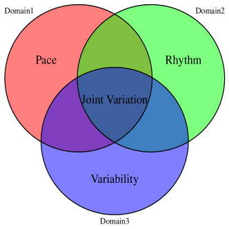
Figure 4: Left Panel: Venn diagram highlighting two main sources of variation: joint (the shaded intersection region) and domain-specific (individual part of each circle). Right Panel: Joint and individual variation explained by each domain from JIVE.

So far in our analysis, we have considered each gait measure separately while performing SOQFR or SOQFR-L to study their association with cognitive performance. However, gait measures are correlated among themselves and conceptually can be placed within one of the five unique gait domains mentioned earlier. The inter-dependence of the metrics within and between the domains can be beneficial in statistical modelling and can be analyzed using JIVE approach with L-moments illustrated in Section 3.2. We focus on domains of Pace (3 features), Rhythm (13 features) and Variability (19 features) as the top performing gait metrics in the SOQFR analysis (see Table Distributional data analysis via quantile functions and its application to modelling digital biomarkers of gait in Alzheimer’s Disease) belong to either of these three domains. Figure 4 (left panel) displays a Venn diagram illustrating a conceptual overlap of joint and individual variation across the three domains.

First, we pre-normalize all the variables (subject-specific L-moments in our case) via z-score transformation $z_{i}=\Phi^{-1}(\hat{F}_{n}(x_{i}))$, where $x_{i}$s are the original features and $\hat{F}_{n}$ is the empirical c.d.f of $\{x_{i}\}_{i=1}^{n}$. Further, all the data blocks are again normalized (centered and scaled) so that data blocks from different domains are comparable as suggested by Lock and others (2013). Applying JIVE (O’Connell and Lock, 2017) and determining the optimal ranks via the permutation test, we get the following ranks: (Joint, Pace, Rhythm, Variability) = $(2,2,7,9)$. Figure 4 (right panel) displays the amount of variation explained by joint and individual components in each of the three domains. Note that JIVE results in significant dimension reduction - reducing the dimension from $140$ (4 L-moments from each of 35 gait metrics) to just $20$. JIVE estimates of the joint and individual structures are shown in Supplementary Figure S7.

We use the JIVE scores, orthogonal by construction, to study the association with cognitive status (mild-AD). Since, we only have a relatively small sample ($n=86$), we further perform variable selection and identify the important JIVE scores using LASSO (Tibshirani, 1996). The selected JIVE scores (joint-PC1, joint-PC2, Pace-PC1, Pace-PC2, Rhythm-PC1, Rhythm-PC2, Rhythm-PC5, Rhythm-PC7, Variability-PC4, Variability-PC7 and Variability-PC9) are used in modelling cognitive status via logistic regression, while adjusting for age and sex. The results are reported in Supplementary Table S6.

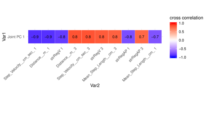
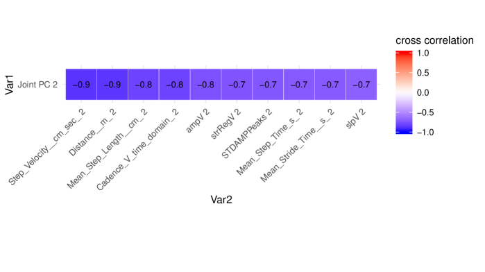
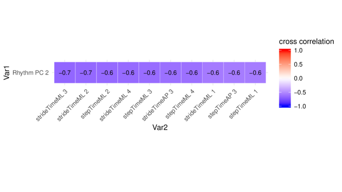
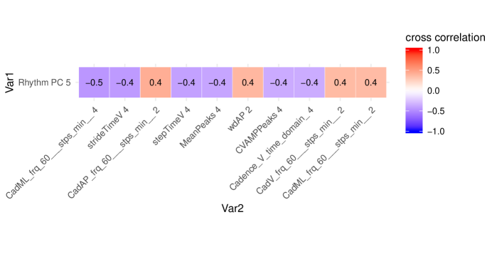
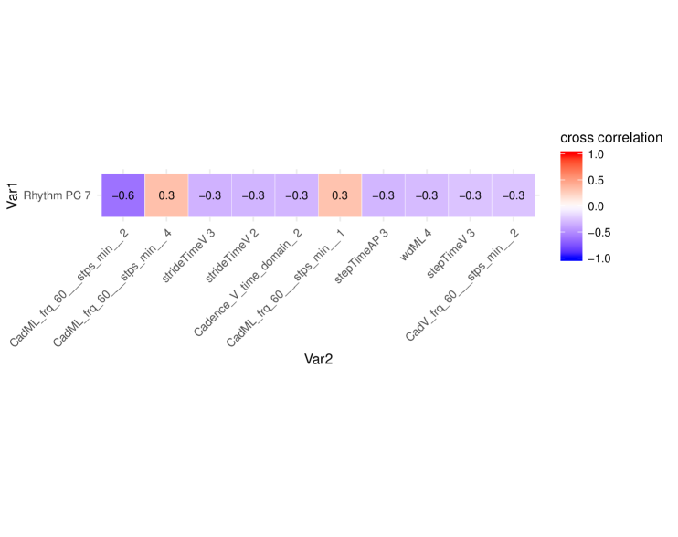
Figure 5: Cross correlation between JIVE PC scores and L-moments. Shown are the top 10 L-moments ranked according to absolute value of correlation with each PC score. “Gait measure $r$” represents $(r)$ th L-moment of the particular gait metric.

To further understand the associations of JIVE PC scores with cognitive function relate them back to the original gait metrics, we use the cross-correlation between the original L-moments and the significant JIVE scores. The top 10 gait metrics (L-moments) ranked according to their correlation with each score are displayed in Figure 5. Joint-PC1, joint-PC2 are found to be positively associated with higher odds of AD. For joint PC-1, the first order L-moments ($L_{1}$) from Pace (step velocity, distance) and Rhythm (stride regularity) are negatively loaded, indicating higher mean value for these variables e.g., step velocity lowers the odds of AD. Similarly, for joint PC-2, the second order L-moments ($L_{2}$) from Pace (step velocity, distance, mean step length) and Rhythm (cadence) are negatively loaded, indicating higher second order L-moments (representing scale) for these variables are associated with a lower risk of AD which matches with our analysis in Section 4.3. The association between cognitive status and Rhythm-PC2, Rhythm-PC5 are found to be negative, whereas Rhythm-PC7 is found to be positively associated. Primarily, higher order L-moments ($L_{2},L_{3},L_{4}$) gait metrics from Rhythm and Variability are loaded on these individual PCs outlining the importance of these domains.

5 Discussion

Distributional data analysis is an emerging area of research in digital medicine that has a large number of diverse applications. There are many ways to represent distributional information including cumulative distribution function, density function, quantile function, and others. Although, all these distributional representations can be re-expressed through each other via differential, integral, inverse, or other more involved transformation, a specific choice for statistical modelling may depend on desirable interpretation and require different analytical machinery. We have proposed to capture distributional nature of wearable data via subject-specific quantile functions and use them or their L-moment representations in SOFR, FGAM, and JIVE methods. As we argue, our approach provide many advantages including intuitive interpretation of results in terms of both quantile levels and L-moments as well as uniform support on $[0,1]$. Additional motivation for the proposed quantile-function approach stems from multiple research efforts aimed at discovering digital biomarkers based on distributional properties of wearable data. Stride-velocity-q95, a 95-percentile of accelerometry-estimated stride velocity, is one of the very first digital biomarkers approved as a secondary endpoint by the European Medicines Agency (EMA), a European counterpart of the Federal Drug Administration in the US (Haberkamp and others, 2019). This measure has been demonstrated to be much more sensitive for tracking longitudinal decline in children with Duchenne muscular distrophy compared to the mean stride-velocity. Another example comes from accelerometry-estimated gait, which is often quantified via user-specific averages, measures of variability (such as standard deviation), and asymmetry (such as skewness) of gait parameters (Hausdorff and others, 2018; Shema-Shiratzky and others, 2020) estimated over a wear-period. Thus, wearable applications actively employ various distributional or quantile based user-specific summaries.

We have demonstrated how proposed approaches provide deeper understanding of the associations between digital gait biomarkers and cognitive functioning in Alzheimer’s disease. Specifically, we showed that quantile functions of gait metrics including step velocity, distance, cadence, stride regularity, mean stride time and mean step time provide higher discrimination between mild-AD and non-AD (CNC) disease status. We also found that second order L-moments capturing subject-specific variability of a few gait parameters are significantly associated with cognitive domains of attention, verbal memory, and executive function. With continuous monitoring of patients with accelerometers and gyroscopes, the method proposed in this manuscript can be adapted to monitor the functional status in Alzheimer’s disease.

These are many more areas that remain to be explored based on the current work. We chose the number of L-moments using PVE criteria. However, similarly to FPCR, it may impose constraints on the flexibility/complexity of estimated $\beta(p)$ and strategies similar to functional penalized regression (Goldsmith and others, 2011) could be explored. In the application of this paper, we have considered one distributional predictor at a time to study associations with the particular outcome of interest. It is plausible to consider several distributional predictors together or perform variable selection within SOQFR (Gertheiss and others, 2013) for a better prediction/classification achievement. It would be also of interest to conceptualize and accommodate distribution-level interactions. One way to do this would be via the inner product of quantile functions expressed in terms of the interactions of corresponding L-moments. Another possible direction of work is to extend the SOQFR model to capture local temporal effects (e.g. for physical activity data) which depends on the time of the day. Beyond distributional aspect of wearable data, there are many other aspects that may be informative. For example, the time of day, the time since the last walking bout, the walking bout duration, and others could be possibly informative for modelling outcomes of interest. Finally, normalization of scales across multiple distributional predictors will need to be deeply studied. For example, quantile function $Q_{i}(p)$ could be normalized within each subject using the transformation $(Q_{i}(p)-Median_{i})/IQR_{i}$ to make scales more comparable across subjects and variables.

6 Software

Illustration of the proposed framework via R (R Core Team, 2018), along with the dataset analyzed, is available on Github at https://github.com/rahulfrodo/DDA.

7 Supplementary Material

Supplementary material is available online at http://biostatistics.oxfordjournals.org.

Figure 1: Displayed are the individual (left two panel) and average (right panel) quantile functions of step velocity for AD (solid) and CNC (dashed).

Table 1: Displayed are the proportion of deviance explained (D.E) by SOQFR and FGAM-QF modelling cognitive status using quantile functions of gait metrics in presence of age and sex. The top 10 metrics (ranked by proportion of deviance explained) have been reported for each of the method. We also report cross-validated (10-fold) AUC (cvAUC) of the models from repeated (B=100) cross-validation. cvAUC from generalized linear models (logit link) using only mean of the gait measures as predictor (along with age and sex) are provided for comparison in the parenthesis.

Variable
(ranked for SOQFR)	D.E
	cvAUC
	Variable
	D.E
	cvAUC
	FGAM-QF
strRegAP	0.58	0.79 (0.74)	Mean_Stride_Time__s_	0.63	0.93 (0.73)
Step_Velocity__cm_sec_	0.50	0.89 (0.80)	Mean_Step_Time_s_	0.63	0.93 (0.73)
Distance__m_	0.49	0.89 (0.80)	strRegAP	0.59	0.83 (0.74)
Cadence_V_time_domain_	0.48	0.90 (0.76)	Step_Velocity__cm_sec_	0.50	0.89 (0.80)
strideTimeV	0.40	0.80 (0.70)	Mean_Step_Length__cm_	0.50	0.83 (0.79)
frqML	0.38	0.84 (0.71)	frqV	0.50	0.86 (0.73)
CV_Step_time	0.38	0.85 (0.68)	stepTimeV	0.50	0.85 (0.70)
frqV	0.37	0.82 (0.73)	strideTimeV	0.50	0.85 (0.70)
Mean_Stride_Time__s_	0.37	0.81 (0.73)	Distance__m_	0.49	0.89 (0.80)
Mean_Step_Time_s_	0.37	0.81 (0.73)	Cadence_V_time_domain_	0.48	0.90 (0.76)

Table 2: The results of SOQFR-L, modelling mild-AD status (adjusted for age and sex) on first four L-moments of stride regularity (Model A1) , step velocity (Model A2) and cadence (Model A3) respectively. Deviance explained using only mean of gait measures (adjusted for age and sex) are provided for comparison in the parenthesis. We also report cross-validated (10-fold) AUC (cvAUC) of the models from repeated (B=100) cross-validation. cvAUC from models using only mean of the gait measures as predictor (along with age and sex) are provided for comparison in the parenthesis.

Model A1 (stride regularity)			Model A2 (step velocity)			Model A3 (cadence)
Coef	est	p-value	Coef	est	p-value	Coef	est	p-value
$\beta_{0}$	4.31	0.17327	$\beta_{0}$	18.203	0.00267	$\beta_{0}$	6.338	0.25626
age	-0.044	0.22957	age	-0.151	0.00836	age	-0.048	0.29464
sex (M)	2.113	0.00015	sex (M)	3.706	$5.11\times 10^{-5}$	sex (M)	2.740	0.00155
$L_{1}$	-0.604	0.85739	$L_{1}$	-0.044	0.16441	$L_{1}$	0.009	0.84854
$L_{2}$	-21.801	0.03457	$L_{2}$	-0.480	0.00127	$L_{2}$	-1.055	$4.2\times 10^{-5}$
$L_{3}$	4.621	0.84022	$L_{3}$	-0.601	0.03620	$L_{3}$	0.002	0.99676
$L_{4}$	12.761	0.63239	$L_{4}$	-0.212	0.61004	$L_{4}$	-0.121	0.90079
Deviance explained	$21.58(15.59)\%$		Deviance explained	$48.75(24.20)\%$		Deviance explained	$45.11(17.73)\%$
cvAUC	$0.74(0.74)$		cvAUC	$0.89(0.80)$		cvAUC	$0.87(0.76)$

Table 3: The results from linear regression models of cognitive scores (ATTN, VM and EF) on first four L-moments of stride regularity, step velocity and cadence, adjusting for age, sex and education. Benchmark models using just age, sex, and education produce adjusted-$R^{2}_{ATTN}=0.163$, $R^{2}_{VM}=0.2489$, $R^{2}_{EF}=0.2754$. We also report cross-validated (10-fold) R-squared of the models from repeated (B=100) cross-validation. Both metrics (adj-Rsq and cv-Rsq) from models using only mean of the gait measures (along with age, sex and education) are provided for comparison in the parenthesis.

Y	Model B1 (stride regularity)			Model B2 (step velocity)			Model B3 (cadence)
ATTN	Coef	est	p-value	Coef	est	p-value	Coef	est	p-value
	$\beta_{0}$	-2.471	0.017	$\beta_{0}$	-1.964	0.089	$\beta_{0}$	0.738	0.591
	age	0.005	0.640	age	0.007	0.507	age	0.001	0.924
	sex (M)	-0.34	0.031	sex (M)	-0.454	0.006	sex (M)	-0.549	0.002
	edu	0.082	0.001	edu	0.069	0.009	edu	0.074	0.004
	$L_{1}$	0.879	0.379	$L_{1}$	0.001	0.897	$L_{1}$	-0.025	0.035
	$L_{2}$	5.879	0.051	$L_{2}$	0.039	0.138	$L_{2}$	0.124	0.004
	$L_{3}$	5.616	0.424	$L_{3}$	0.015	0.756	$L_{3}$	-0.137	0.122
	$L_{4}$	-6.456	0.415	$L_{4}$	-0.004	0.961	$L_{4}$	0.025	0.882
	adj-Rsq	0.240 (0.172)		adj-Rsq	0.192 (0.173)		adj-Rsq	0.226 (0.154)
	cv-Rsq	0.273 (0.211)		cv-Rsq	0.214 (0.209)		cv-Rsq	0.264 (0.209)
VM	$\beta_{0}$	-4.469	0.036	$\beta_{0}$	-3.283	0.159	$\beta_{0}$	0.655	0.819
	age	0.001	0.973	age	0.009	0.707	age	-0.009	0.666
	sex (M)	-1.296	$1\times 10^{-4}$	sex (M)	-1.591	$5.8\times 10^{-6}$	sex (M)	-1.583	$3.4\times 10^{-5}$
	edu	0.171	0.001	edu	0.119	0.025	edu	0.123	0.022
	$L_{1}$	1.173	0.571	$L_{1}$	$7.4\times 10^{-6}$	0.999	$L_{1}$	-0.030	0.213
	$L_{2}$	17.118	0.007	$L_{2}$	0.131	0.014	$L_{2}$	0.315	0.001
	$L_{3}$	11.616	0.424	$L_{3}$	0.094	0.350	$L_{3}$	-0.158	0.389
	$L_{4}$	4.214	0.797	$L_{4}$	0.119	0.531	$L_{4}$	0.215	0.545
	adj-Rsq	0.365 (0.251)		adj-Rsq	0.356 (0.269)		adj-Rsq	0.346 (0.246)
	cv-Rsq	0.390 (0.311)		cv-Rsq	0.390 (0.332)		cv-Rsq	0.383 (0.317)
EF	$\beta_{0}$	-3.307	0.048	$\beta_{0}$	-3.623	0.048	$\beta_{0}$	0.844	0.698
	age	0.004	0.814	age	0.016	0.389	age	-0.002	0.912
	sex (M)	-1.140	$2.4\times 10^{-5}$	sex (M)	-1.329	$1.5\times 10^{-6}$	sex (M)	-1.368	$3.4\times 10^{-6}$
	edu	0.134	0.001	edu	0.108	0.009	edu	0.103	0.012
	$L_{1}$	-0.402	0.804	$L_{1}$	0.005	0.697	$L_{1}$	-0.036	0.053
	$L_{2}$	15.992	0.001	$L_{2}$	0.087	0.034	$L_{2}$	0.294	$2.8\times 10^{-5}$
	$L_{3}$	-3.396	0.765	$L_{3}$	0.051	0.512	$L_{3}$	-0.264	0.061
	$L_{4}$	-1.960	0.879	$L_{4}$	-0.064	0.664	$L_{4}$	0.442	0.104
	adj-Rsq	0.377 (0.280)		adj-Rsq	0.376 (0.302)		adj-Rsq	0.397 (0.271)
	cv-Rsq	0.414 (0.347)		cv-Rsq	0.425 (0.358)		cv-Rsq	0.441 (0.345)

References

- Aitchison (1982) Aitchison, John. (1982). The statistical analysis of compositional data. Journal of the Royal Statistical Society: Series B (Methodological) 44(2), 139–160.
- Alzheimer’s Association (2020) Alzheimer’s Association. (2020). 2020 alzheimer’s disease facts and figures. Alzheimer’s & Dementia 16(3), 391–460.
- Augustin and others (2017) Augustin, Nicole H, Mattocks, Calum, Faraway, Julian J, Greven, Sonja and Ness, Andy R. (2017). Modelling a response as a function of high-frequency count data: The association between physical activity and fat mass. Statistical methods in medical research 26(5), 2210–2226.
- Bakrania and others (2017) Bakrania, Kishan, Yates, Thomas, Edwardson, Charlotte L, Bodicoat, Danielle H, Esliger, Dale W, Gill, Jason MR, Kazi, Aadil, Velayudhan, Latha, Sinclair, Alan J and Sattar, Naveed. (2017). Associations of moderate-to-vigorous-intensity physical activity and body mass index with glycated haemoglobin within the general population: a cross-sectional analysis of the 2008 health survey for england. BMJ Open 7(4), e014456.
- Bigot and others (2018) Bigot, Jérémie, Gouet, Raúl, Klein, Thierry and Lopez, Alfredo. (2018). Upper and lower risk bounds for estimating the wasserstein barycenter of random measures on the real line. Electronic Journal of Statistics 12(2), 2253–2289.
- Chen and others (2021) Chen, Yaqing, Lin, Zhenhua and Müller, Hans-Georg. (2021). Wasserstein regression. Journal of the American Statistical Association (just-accepted), 1–40.
- Dryden and Mardia (2016) Dryden, Ian L and Mardia, Kanti V. (2016). Statistical shape analysis: with applications in R, Volume 995. John Wiley & Sons.
- Dumuid and others (2020) Dumuid, Dorothea, Pedišić, Željko, Palarea-Albaladejo, Javier, Martín-Fernández, Josep Antoni, Hron, Karel and Olds, Timothy. (2020). Compositional data analysis in time-use epidemiology: what, why, how. International Journal of Environmental Research and Public Health 17(7), 2220.
- Dumuid and others (2019) Dumuid, Dorothea, Pedišić, Željko, Stanford, Tyman Everleigh, Martín-Fernández, Josep-Antoni, Hron, Karel, Maher, Carol A, Lewis, Lucy K and Olds, Timothy. (2019). The compositional isotemporal substitution model: a method for estimating changes in a health outcome for reallocation of time between sleep, physical activity and sedentary behaviour. Statistical Methods in Medical Research 28(3), 846–857.
- Gertheiss and others (2013) Gertheiss, Jan, Maity, Arnab and Staicu, Ana-Maria. (2013). Variable selection in generalized functional linear models. Stat 2(1), 86–101.
- Ghodrati and Panaretos (2021) Ghodrati, Laya and Panaretos, Victor M. (2021). Distribution-on-distribution regression via optimal transport maps. arXiv preprint arXiv:2104.09418.
- Gilchrist (2000) Gilchrist, Warren. (2000). Statistical modelling with quantile functions. CRC Press.
- Goldsmith and others (2011) Goldsmith, Jeff, Bobb, Jennifer, Crainiceanu, Ciprian M, Caffo, Brian and Reich, Daniel. (2011). Penalized functional regression. Journal of Computational and Graphical Statistics 20(4), 830–851.
- Goldsmith and others (2016) Goldsmith, Jeff, Liu, Xinyue, Jacobson, Judith and Rundle, Andrew. (2016). New insights into activity patterns in children, found using functional data analyses. Medicine and Science in Sports and Exercise 48(9), 1723.
- Goldsmith and others (2018) Goldsmith, Jeff, Scheipl, Fabian, Huang, Lei, Wrobel, Julia, Gellar, Jonathan, Harezlak, Jaroslaw, McLean, Mathew W., Swihart, Bruce, Xiao, Luo, Crainiceanu, Ciprian and others. (2018). refund: Regression with Functional Data. R package version 0.1-17.
- Goldsmith and others (2015) Goldsmith, Jeff, Zipunnikov, Vadim and Schrack, Jennifer. (2015). Generalized multilevel function-on-scalar regression and principal component analysis. Biometrics 71(2), 344–353.
- Haberkamp and others (2019) Haberkamp, Marion, Moseley, Jane, Athanasiou, Dimitrios, de Andres-Trelles, Fernando, Elferink, André, Rosa, Mário Miguel and Magrelli, Armando. (2019). European regulators’ views on a wearable-derived performance measurement of ambulation for duchenne muscular dystrophy regulatory trials. Neuromuscular Disorders 29(7), 514–516.
- Hausdorff and others (2018) Hausdorff, Jeffrey M, Hillel, Inbar, Shustak, Shiran, Del Din, Silvia, Bekkers, Esther MJ, Pelosin, Elisa, Nieuwhof, Freek, Rochester, Lynn and Mirelman, Anat. (2018). Everyday stepping quantity and quality among older adult fallers with and without mild cognitive impairment: initial evidence for new motor markers of cognitive deficits? The Journals of Gerontology: Series A 73(8), 1078–1082.
- Hebert and others (2013) Hebert, Liesi E, Weuve, Jennifer, Scherr, Paul A and Evans, Denis A. (2013). Alzheimer disease in the united states (2010–2050) estimated using the 2010 census. Neurology 80(19), 1778–1783.
- Hosking (1990) Hosking, Jonathan RM. (1990). L-moments: Analysis and estimation of distributions using linear combinations of order statistics. Journal of the Royal Statistical Society: Series B (Methodological) 52(1), 105–124.
- Hron and others (2016) Hron, Karel, Menafoglio, Alessandra, Templ, Matthias, Hruzova, K and Filzmoser, Peter. (2016). Simplicial principal component analysis for density functions in bayes spaces. Computational Statistics & Data Analysis 94, 330–350.
- Huang and others (2019) Huang, Lei, Bai, Jiawei, Ivanescu, Andrada, Harris, Tamara, Maurer, Mathew, Green, Philip and Zipunnikov, Vadim. (2019). Multilevel matrix-variate analysis and its application to accelerometry-measured physical activity in clinical populations. Journal of the American Statistical Association 114(526), 553–564.
- Ichimura (1991) Ichimura, Hidehiko. (1991). Semiparametric least squares (sls) and weighted sls estimation of single-index models.
- Irpino and Verde (2013) Irpino, Antonio and Verde, Rosanna. (2013). A metric based approach for the least square regression of multivariate modal symbolic data. In: Statistical Models for Data Analysis. Springer, pp. 161–169.
- Kourtis and others (2019) Kourtis, Lampros C, Regele, Oliver B, Wright, Justin M and Jones, Graham B. (2019). Digital biomarkers for alzheimer’s disease: the mobile/wearable devices opportunity. NPJ Digital Medicine 2(1), 1–9.
- Lock and others (2013) Lock, Eric F, Hoadley, Katherine A, Marron, James Stephen and Nobel, Andrew B. (2013). Joint and individual variation explained (jive) for integrated analysis of multiple data types. The Annals of Applied Statistics 7(1), 523.
- Marx and Eilers (1999) Marx, Brian D and Eilers, Paul HC. (1999). Generalized linear regression on sampled signals and curves: a p-spline approach. Technometrics 41(1), 1–13.
- Matabuena and Petersen (2021) Matabuena, Marcos and Petersen, Alex. (2021). Distributional data analysis with accelerometer data in a nhanes database with nonparametric survey regression models. arXiv.
- Matabuena and others (2021) Matabuena, Marcos, Petersen, Alexander, Vidal, Juan C and Gude, Francisco. (2021). Glucodensities: a new representation of glucose profiles using distributional data analysis. Statistical Methods in Medical Research 30(6), 1445–1464.
- Mc Ardle and others (2020) Mc Ardle, Ríona, Del Din, Silvia, Galna, Brook, Thomas, Alan and Rochester, Lynn. (2020). Differentiating dementia disease subtypes with gait analysis: feasibility of wearable sensors? Gait & Posture 76, 372–376.
- Mc Ardle and others (2019) Mc Ardle, Ríona, Galna, Brook, Donaghy, Paul, Thomas, Alan and Rochester, Lynn. (2019). Do alzheimer’s and lewy body disease have discrete pathological signatures of gait? Alzheimer’s & Dementia 15(10), 1367–1377.
- McKeague and Chang (2019) McKeague, Ian and Chang, Hsin-wen. (2019). Functional data analysis for activity profiles from wearable devices. https://www.ima.umn.edu/materials/2019-2020/DW9.16-17.19/28237/talk_Minneapolis.pdf.
- McLean and others (2014) McLean, Mathew W, Hooker, Giles, Staicu, Ana-Maria, Scheipl, Fabian and Ruppert, David. (2014). Functional generalized additive models. Journal of Computational and Graphical Statistics 23(1), 249–269.
- Morris (2015) Morris, Jeffrey S. (2015). Functional regression. Annual Review of Statistics and Its Application 2, 321–359.
- Morris and others (2006) Morris, Jeffrey S, Arroyo, Cassandra, Coull, Brent A, Ryan, Louise M, Herrick, Richard and Gortmaker, Steven L. (2006). Using wavelet-based functional mixed models to characterize population heterogeneity in accelerometer profiles: a case study. Journal of the American Statistical Association 101(476), 1352–1364.
- Müller and Yao (2008) Müller, Hans-Georg and Yao, Fang. (2008). Functional additive models. Journal of the American Statistical Association 103(484), 1534–1544.
- O’Connell and Lock (2017) O’Connell, Michael J. and Lock, Eric F. (2017). r.jive: Perform JIVE Decomposition for Multi-Source Data. R package version 2.1.
- Panaretos and Zemel (2020) Panaretos, Victor M and Zemel, Yoav. (2020). An invitation to statistics in Wasserstein space. Springer Nature.
- Parzen (2004) Parzen, Emanuel. (2004). Quantile probability and statistical data modeling. Statistical Science 19(4), 652–662.
- Petersen and Müller (2016) Petersen, Alexander and Müller, Hans-Georg. (2016). Functional data analysis for density functions by transformation to a hilbert space. The Annals of Statistics 44(1), 183–218.
- Petersen and others (2021) Petersen, Alexander, Zhang, Chao and Kokoszka, Piotr. (2021). Modeling probability density functions as data objects. Econometrics and Statistics.
- Powley (2013) Powley, Bradford W. (2013). Quantile function methods for decision analysis [Ph.D. Thesis]. Stanford University.
- R Core Team (2018) R Core Team. (2018). R: A Language and Environment for Statistical Computing. R Foundation for Statistical Computing, Vienna, Austria.
- Reider and others (2020) Reider, Lisa, Bai, Jiawei, Scharfstein, Daniel O and Zipunnikov, Vadim. (2020). Methods for step count data: Determining “valid” days and quantifying fragmentation of walking bouts. Gait & Posture 81, 205–212.
- Reiss and others (2017) Reiss, Philip T, Goldsmith, Jeff, Shang, Han Lin and Ogden, R Todd. (2017). Methods for scalar-on-function regression. International Statistical Review 85(2), 228–249.
- Shema-Shiratzky and others (2020) Shema-Shiratzky, Shirley, Hillel, Inbar, Mirelman, Anat, Regev, Keren, Hsieh, Katherine L, Karni, Arnon, Devos, Hannes, Sosnoff, Jacob J and Hausdorff, Jeffrey M. (2020). A wearable sensor identifies alterations in community ambulation in multiple sclerosis: contributors to real-world gait quality and physical activity. Journal of Neurology 267(7), 1912–1921.
- Stoker (1986) Stoker, Thomas M. (1986). Consistent estimation of scaled coefficients. Econometrica: Journal of the Econometric Society, 1461–1481.
- Takemura (1983) Takemura, Akimichi. (1983). Orthogonal expansion of quantile function and components of the shapiro-francia statistic. Technical Report, Stanford University CA Department of Statistics.
- Talská and others (2021) Talská, Renáta, Hron, Karel and Grygar, Tomáš Matys. (2021). Compositional scalar-on-function regression with application to sediment particle size distributions. Mathematical Geosciences, 1–29.
- Tibshirani (1996) Tibshirani, Robert. (1996). Regression shrinkage and selection via the lasso. Journal of the Royal Statistical Society: Series B (Methodological) 58(1), 267–288.
- Van den Boogaart and others (2014) Van den Boogaart, Karl Gerald, Egozcue, Juan José and Pawlowsky-Glahn, Vera. (2014). Bayes hilbert spaces. Australian & New Zealand Journal of Statistics 56(2), 171–194.
- Varma and others (2017) Varma, Vijay R, Dey, Debangan, Leroux, Andrew, Di, Junrui, Urbanek, Jacek, Xiao, Luo and Zipunnikov, Vadim. (2017). Re-evaluating the effect of age on physical activity over the lifespan. Preventive Medicine 101, 102–108.
- Varma and others (2021) Varma, Vijay R, Ghosal, Rahul, Hillel, Inbar, Volfson, Dmitri, Weiss, Jordan, Urbanek, Jacek, Hausdorff, Jeffrey M., Zipunnikov, Vadim and Watts, Amber. (2021). Continuous gait monitoring discriminates community dwelling mild ad from cognitively normal controls. Alzheimer’s & Dementia: Translational Research & Clinical Interventions 7(1), e12131.
- Varma and Watts (2017) Varma, Vijay R and Watts, Amber. (2017). Daily physical activity patterns during the early stage of alzheimer’s disease. Journal of Alzheimer’s Disease 55(2), 659–667.
- Verde and Irpino (2010) Verde, Rosanna and Irpino, Antonio. (2010). Ordinary least squares for histogram data based on wasserstein distance. In: Proceedings of COMPSTAT’2010. Springer, pp. 581–588.
- Wang and Yang (2009) Wang, Li and Yang, Lijian. (2009). Spline estimation of single-index models. Statistica Sinica 19(2), 765–783.
- Weiss and others (2014) Weiss, Aner, Herman, Talia, Giladi, Nir and Hausdorff, Jeffrey M. (2014). Objective assessment of fall risk in parkinson’s disease using a body-fixed sensor worn for 3 days. PloS one 9(5), e96675.
- Wood (2017) Wood, Simon N. (2017). Generalized additive models: an introduction with R. CRC press.
- Wood and others (2016) Wood, Simon N, Pya, Natalya and Säfken, Benjamin. (2016). Smoothing parameter and model selection for general smooth models. Journal of the American Statistical Association 111(516), 1548–1563.
- Wrobel and others (2019) Wrobel, Julia, Zipunnikov, Vadim, Schrack, Jennifer and Goldsmith, Jeff. (2019). Registration for exponential family functional data. Biometrics 75(1), 48–57.
- Xiao and others (2015) Xiao, Luo, Huang, Lei, Schrack, Jennifer A, Ferrucci, Luigi, Zipunnikov, Vadim and Crainiceanu, Ciprian M. (2015). Quantifying the lifetime circadian rhythm of physical activity: a covariate-dependent functional approach. Biostatistics 16(2), 352–367.
- Yang (2020) Yang, Hojin. (2020). Random distributional response model based on spline method. Journal of Statistical Planning and Inference 207, 27–44.
- Yang and others (2020) Yang, Hojin, Baladandayuthapani, Veerabhadran, Rao, Arvind UK and Morris, Jeffrey S. (2020). Quantile function on scalar regression analysis for distributional data. Journal of the American Statistical Association 115(529), 90–106.
- Yogev-Seligmann and others (2008) Yogev-Seligmann, Galit, Hausdorff, Jeffrey M and Giladi, Nir. (2008). The role of executive function and attention in gait. Movement Disorders 23(3), 329–342.
- Zhang and Müller (2011) Zhang, Zhen and Müller, Hans-Georg. (2011). Functional density synchronization. Computational Statistics & Data Analysis 55(7), 2234–2249.