Bertsimas and Digalakis Jr. and Li and Skali Lami

Slowly Varying Regression under Sparsity

Slowly Varying Regression under Sparsity

Dimitris Bertsimas Sloan School of Management, Massachusetts Institute of Technology, Cambridge, MA, USA Vassilis Digalakis Jr Department of Information Systems and Operations Management, HEC Paris, 78350 Jouy-en-Josas, France
Operations Research Center, Massachusetts Institute of Technology, Cambridge, MA, USA Michael Lingzhi Li Technology and Operations Management Unit, Harvard Business School, Boston, MA, USA Omar Skali Lami McKinsey & Company, Boston, MA, USA

We introduce the framework of slowly varying regression under sparsity, which allows sparse regression models to vary slowly and sparsely. We formulate the problem of parameter estimation as a mixed integer optimization problem and demonstrate that it can be reformulated exactly as a binary convex optimization problem through a novel relaxation. The relaxation utilizes a new equality on Moore-Penrose inverses that convexifies the non-convex objective function while coinciding with the original objective on all feasible binary points. This allows us to solve the problem significantly more efficiently and to provable optimality using a cutting plane-type algorithm. We develop a highly optimized implementation of such algorithm, which substantially improves upon the asymptotic computational complexity of a straightforward implementation. We further develop a fast heuristic method that is guaranteed to produce a feasible solution and, as we empirically illustrate, generates high-quality warm-start solutions for the binary optimization problem. To tune the framework’s hyperparameters, we propose a practical procedure relying on binary search that, under certain assumptions, is guaranteed to recover the true model parameters. We show, on both synthetic and real-world datasets, that the resulting algorithm outperforms competing formulations in comparable times across a variety of metrics including estimation accuracy, predictive power, and computational time, and is highly scalable, enabling us to train models with 10,000s of parameters. We make our implementation available open-source at https://github.com/vvdigalakis/SSVRegression.git.

Slowly Varying Regression, Sparsity, Mixed Integer Optimization, Binary Convex Relaxation

1 Introduction

We introduce the framework of slowly varying regression under sparsity (SSVR), which addresses a large number of problems in machine learning where the underlying model is sparse and varies slowly and sparsely. This in particular includes problems with temporally or spatially varying structure. For example, in the temporal case, the factors important in predicting the energy consumption in a building can vary depending on the hour of the day or the period of the year. In the spatial case, the factors that affect house prices can differ by neighborhood.

In both cases, a modeler may be motivated to use different models for each time period, spatial area, or, more generally, “vertex.” However, using separate models ignores the innate dependence across different vertices (e.g., energy consumption is strongly affected by daily and seasonal patterns) and creates interpretability issues if the separate models turn out to be notably different. Further, separate models require substantial data to be available for each vertex, which is often difficult. In this work, we address the need to capture this slowly and sparsely varying structure in a global way.

1.1 Slowly Varying Regression under Sparsity: An Initial Formulation

Formally, we consider a multiple regression problem with $N$ cases having features $\bm{X}^{1},\dots,\bm{X}^{T}$, where $\bm{X}^{t}\in\mathbb{R}^{N\times D}$ for $t\in[T]:=\{1,\dots,T\},$ and outcomes $\bm{y}^{1},\dots,\bm{y}^{T}$, where $\bm{y}^{t}\in\mathbb{R}^{N}$ for $t\in[T]$. An SSVR model assumes that the regression coefficients and relevant features (i.e., features that correspond to nonzero coefficients) change slowly between pairs of regressions $(s,t)\in E\subseteq[T]\times[T]$ that are considered similar. Two prominent applications include temporally varying regression and spatially varying regression. In the temporal case, the regressions are scattered over $T$ consecutive time periods, and regressions between two consecutive time periods are considered to be similar. In the spatial case, the regressions are conducted over $T$ spatial areas, some of which are adjacent to each other, and it is common to assume that regressions in adjacent areas have to be similar. More generally, the $T$ regressions are conducted over a graph $G$ with vertices $V$ of size $|V|=T$. For $v,w\in V$, the edge $(v,w)$ is in the set of edges $E$ if and only if $v$ and $w$ are considered to be similar. Figure 1 presents examples of similarity graphs.

Figure 1: Examples of similarity graphs. In the temporal case (left), the different regressions are applied across T consecutive time periods. (Such examples are considered in Section 9.1.) In the spatial case (right), the different regressions are applied across 7 spatial areas (S, E, W, NE, NW, N, NN) with the given similarity structure. (The graph corresponds to one of the experiments described in Section 9.2.)

The SSVR problem can be formulated as below:

$$\underset{\bm{\beta}^{1},\cdots,\bm{\beta}^{T}}{\min}\quad \sum_{t=1}^{T}\left\|\bm{y}^{t}-\bm{X}^{t}\bm{\beta}^{t}\right\|_{2}^{2}+\lambda_{\beta}\sum_{t=1}^{T}\|\bm{\beta}^{t}\|_{2}^{2}+\lambda_{\delta}\sum_{(s,t)\in E}\|\bm{\beta}^{t}-\bm{\beta}^{s}\|_{2}^{2}$$ (1)

s.t. $$\left|\text{Supp}(\bm{\beta}^{t})\right|\leq K_{\text{L}},\quad\forall t\in[T],$$ (2)

$$\left|\bigcup_{t=1}^{T}\text{Supp}(\bm{\beta}^{t})\right|\leq K_{\text{G}},$$ (3)

$$\sum_{(s,t)\in E}\left|\text{Supp}(\bm{\beta}^{t})\triangle\text{Supp}(\bm{\beta}^{s})\right|\leq K_{\text{C}},$$ (4)

where $\text{Supp}(\bm{\beta})$ denotes the set that corresponds to the support of vector $\bm{\beta}$ and $S_{1}\triangle S_{2}$ denotes the symmetric difference of sets $S_{1},S_{2}$. The objective function (1) penalizes both the least-squares loss of the $T$ regressions and the $\ell_{2}$ coefficient distance between regressions that are similar with magnitude $\lambda_{\delta}$. We also introduce a further $\ell_{2}$ regularization term of magnitude $\lambda_{\beta}$ for robustness purposes (see, e.g., Xu et al. (2009)). There are three types of constraints on the regression coefficients $\bm{\beta}^{t}$:

• Local Sparsity: Each regression has at most $K_{\text{L}}$ relevant features (constraint (2)).

• Global Sparsity: There are at most $K_{\text{G}}$ relevant features across all $T$ regressions (constraint (3)).

• Sparsely Varying Support: There is a difference of at most $K_{\text{C}}$ relevant features among similar regressions $s,t$ across all pairs of similar regressions (constraint (4)).

For consistency, $K_{\text{L}},K_{\text{G}},K_{\text{C}}$ satisfy $K_{\text{L}}\leq K_{\text{G}}\leq D$ and $K_{\text{C}}\leq 2K_{\text{L}}T$ and $2(K_{\text{G}}-K_{\text{L}})\leq K_{\text{C}}$. This exact formulation is generally considered infeasible beyond toy scales ($D\leq 10^{2},\ T\leq 10$) due to the combinatorial complexity of the sparsity constraints. Therefore, many authors have proposed various relaxations in order to solve variants of this problem, including fused lasso (Tibshirani et al. 2005) and sum-of-norms regularization (Ohlsson et al. 2010); we review such approaches in Section 1.3. Our key contribution in this paper is to show that this general problem can be reformulated as a binary convex optimization problem, which then can be solved efficiently using a cutting plane-type algorithm. This reformulation is primarily enabled by an exact smooth relaxation of the solution under sparsity constraints, which, to the best of our knowledge, has not appeared in prior literature. Furthermore, we discuss in Section 1.4 how the reformulation directly extends to any sparse quadratic convex problem of a general form, making the relaxation generally applicable.

1.2 Contributions and Outline

We now more concretely summarize our contributions from a modeling, theoretical, algorithmic, and computational (practitioner’s) perspective:

• From a modeling standpoint, we introduce the slowly varying regression under sparsity framework, which addresses regression problems with sparse and slowly varying structure.

• From a theoretical standpoint, we propose a new way of solving the underlying optimization problem, which extends to a more general class of sparse quadratic problems. We reformulate the problem exactly as a binary convex optimization problem through a novel relaxation of the objective function. The proposed relaxation relies upon a new equality on Moore-Penrose inverses that convexifies the nonconvex objective function while coinciding on all feasible binary points.

• From an algorithmic standpoint, firstly, leveraging the convexity of the reformulated problem, we develop a cutting plane-type algorithm that enables us to solve the binary convex optimization problem at hand to provable optimality. By exploiting the structure of the problem, we efficiently implement the proposed algorithm and substantially improve upon the asymptotic computational complexity of a straightforward implementation. Secondly, we develop a fast heuristic algorithm, which is guaranteed to produce a feasible solution and, as we empirically show, computes high-quality, warm-start solutions to the binary convex optimization problem. Thirdly, we propose a practical hyperparameter tuning procedure relying on binary search that, under certain assumptions, is guaranteed to recover the true model hyperparameters.

• From a computational standpoint, we thoroughly evaluate the proposed method on both synthetic and real-world data. We show that the proposed algorithm outperforms competing formulations across a variety of metrics including estimation accuracy, predictive power, and computational time, and is highly scalable, enabling us to train models with 10,000s of parameters. In real-world experiments, we further illustrate how the resulting SSVR model can provide insights into the problem at hand. We make our implementation available open-source at https://github.com/vvdigalakis/SSVRegression.git. To facilitate the use of the proposed framework by practitioners, all proposed algorithms can be run through a single line of code, and the learned models are provided in an intuitive and interpretable way.

The outline of the paper is as follows. In the remainder of Section 1, we summarize the relevant literature. In Section 2, we formulate the SSVR problem as a mixed-integer optimization problem. In Section 3, we develop the proposed relaxation of the objective function and reformulate the problem exactly as a binary convex optimization problem. In Section 4, we explore the properties of the proposed relaxation, build intuition on why it works, and studiy how it can be extended to general quadratic models. In Section 5, we develop the proposed exact cutting plane type algorithm and discuss how to efficiently implement it. In Section 6, we design the proposed fast heuristic algorithm. In Section 7, we explain how to tune the SSVR model practically, while also providing theoretical guarantees albeit in limited scenarios. Finally, in Sections 8 and 9, we present our experimental evaluations on synthetic and real-world data, respectively.

1.3 Relevant Literature: Slowly Varying Regression

The practical relevance of the notion of slowly (or smoothly) varying regression is evident by the significant amount of impactful work in the field, dating back to at least Hastie and Tibshirani (1993), who study linear regression models whose coefficients are allowed to change smoothly with the value of other variables, and Bertsimas et al. (1999), who solve the nonparametric regression estimation problem when the underlying regression function is Lipschitz continuous; see, e.g., the book by Eubank (1999) for a comprehensive review and e.g. Phillips (2007), Chen et al. (2020) for applications in Econometrics and Electronics.

The popularity of slowly varying regression models peaked following the work of Tibshirani et al. (2005) on the fused lasso, which proposed to augment the standard lasso (Tibshirani 1996) objective with an $\ell_{1}$ penalty term on the difference between successive regression coefficients $|\beta^{t}-\beta^{t-1}|$ to account for pairwise similarity. The algorithms for solving the resulting problems were improved by many works including (Tibshirani and Taylor 2011, Wytock et al. 2014) while other works considered different convex regularizers or extended the formulation to other settings such as change point detection (Alaíz et al. 2013, Rojas and Wahlberg 2014, Bleakley and Vert 2011).

The works that are most closely related to ours include the sum-of-norms regularization approaches by Ohlsson et al. (2010), Hallac et al. (2015, 2017), the total variation regularization approach by Wytock (2014), and the heuristic splicing approach by Zhang et al. (2023). Ohlsson et al. (2010), in particular, consider the time-varying linear regression optimization problem and their work can naturally be extended to the (more general) graph case that we consider in this paper as follows:

$$\underset{\bm{\beta}^{1},\cdots,\bm{\beta}^{T}}{\min}\quad\sum_{t=1}^{T}\left\|\bm{y}^{t}-\bm{X}^{t}\bm{\beta}^{t}\right\|_{2}^{2}+\lambda_{\delta}\sum_{(s,t)\in E}\|\bm{\beta}^{t}-\bm{\beta}^{s}\|_{p},$$ (5)

where $p\in\{1,2\}$. Our work significantly differs from this line of work by exactly imposing sparsity and sparse variation in the coefficients, hence providing more control to the modeler, and, further, by utilizing a smooth $\ell_{2}$ penalty term on the difference between the regression coefficients $\|\bm{\beta}^{t}-\bm{\beta}^{s}\|_{2}^{2}$.

Another stream of related work in the application of spatially varying regression are spatially varying coefficient (SVC) models. Instead of imposing a strict constraint on the degree of variability, SVC models focus on identifying the heterogeneity in coefficient estimates varying across space. Notable methods include the spatial expansion method (Casetti 1972), geographically weighted regression (Brunsdon et al. 1996), and Bayesian SVC models (Besag et al. 1991).

1.4 Relevant Literature: Solving Sparse Quadratic Models

Problems with sparsity constraints have long been of interest in many areas ranging from machine learning to facility location and portfolio selection, as sparsity improves robustness to data noise and increases interpretability for better decision-making. However, due to their combinatorial complexity, it has long been thought that exact sparse formulations are not scalable, and $\ell_{1}$ regularization formulations (e.g. fused lasso in Section 1.3) have been widely used as surrogates.

In recent years, a growing volume of work has challenged the aforementioned paradigm. Bertsimas et al. (2016), Bertsimas and Van Parys (2020), Hazimeh et al. (2022) solve standard sparse regression problems with design matrix $\bm{X}\in\mathbb{R}^{N\times D}$, responses $\bm{y}\in\mathbb{R}^{N}$, and $\ell_{2}$ regularization, outlined as

$$\min_{\bm{\beta}:\|\bm{\beta}\|_{0}\leq K}\frac{1}{2}\|\bm{y}-\bm{X}\bm{\beta}\|_{2}^{2}+\lambda_{\beta}\|\bm{\beta}\|_{2}^{2},$$ (6)

at scale, using techniques from mixed-integer optimization. Beyond sparse regression, Wei et al. (2022) study the convexification of a class of convex optimization problems with indicator variables and combinatorial constraints on the indicators, whereas, in a recent work motivated by probabilistic graphical models, Liu et al. (2023) study convex quadratic optimization problems with indicator variables when the matrix defining the quadratic term in the objective is sparse.

The work that is most closely related to ours is by Bertsimas and Van Parys (2020), who utilize binary variables $\bm{z}\in\{0,1\}^{D}$ and reformulate Problem (6) as

$$\min_{\bm{z}\in\{0,1\}^{D},\sum_{i=1}^{D}z_{i}\leq K}\min_{\bm{\beta}}\frac{1}{2}\|\bm{y}-\bm{X}\bm{Z}\bm{\beta}\|_{2}^{2}+\lambda_{\beta}\|\bm{\beta}\|_{2}^{2},$$ (7)

where $\bm{Z}=\operatorname{Diag}(z_{1},\dots,z_{D})$. The authors then show that the inner minimization problem can be solved in a closed form that results in a convex binary formulation for the outer problem:

$$\min_{\bm{z}\in\{0,1\}^{D},\sum_{i=1}^{D}z_{i}\leq K}\bm{y}^{T}\left(\bm{I}_{N}+\frac{1}{2\lambda_{\beta}}\sum_{i=1}^{D}z_{i}\bm{X}_{i}\bm{X}_{i}^{T}\right)^{-1}\bm{y},$$ (8)

where $\bm{X}_{i}$ is the $i$th column of design matrix $\bm{X}$. The resulting problem can then be solved efficiently to very large scales ($N,D\approx 10^{4}$) using a cutting plane-type algorithm. This significant breakthrough raised the limits of scaling exact sparse methods by multiple orders of magnitude. However, the transformation presented above seems to be quite fortuitous. For example, the reformulation in Bertsimas and Van Parys (2020) relied on rewriting $\bm{\beta}$ as $\bm{Z}\bm{\beta}$ in the first term but not the second term of Equation (7). There appears to be no systematic reason why doing so is necessary to result in the final convex binary formulation in Equation (8), and even fewer hints on how we could systematically apply this methodology to other problems.

This paper aims to uncover the underlying key ingredients to allow such transformations through the study of the SSVR problem, which is a generalization of the standard sparse regression problem of Equation (6). Moreover, the framework we present here directly extends to any sparse quadratic convex problem of the form

$$\min_{\bm{x}\in\mathcal{X}}\quad\frac{1}{2}\bm{x}^{T}(\bm{M}+\lambda\bm{I})\bm{x}-\bm{\mu}^{T}\bm{x},$$ (9)

where $\bm{\mu}\in\mathbb{R}^{D}$, $\bm{x}\in\mathbb{R}^{D}$ are the decision variables, $\bm{M}\in\mathbb{R}^{D\times D}$ is any positive semidefinite matrix, and $\mathcal{X}$ is the feasible set with sparsity-imposing constraints, e.g. $\mathcal{X}=\{\bm{x}\in\mathbb{R}^{D}:\|\bm{x}\|_{0}\leq K\}$.

Overall, the proposed framework lies between Bertsimas and Van Parys (2020) and Bertsimas et al. (2021). On one extreme, we consider a general quadratic regression framework that contains the sparse regression problem in Bertsimas and Van Parys (2020) as a special case and draw insights from optimization and convex relaxations to efficiently solve the resulting inner problem. On the other extreme, Bertsimas et al. (2021) investigate general sparse mixed-integer optimization problems with logical constraints and develop an outer approximation scheme whereby the solution to the inner problem involves solving an optimization problem in each iteration; in contrast, we focus on sparse mixed-integer optimization problems where the inner problem is an unconstrained quadratic optimization problem and develop a general efficient procedure for optimizing the resulting problem.

2 An MIO Formulation

In this section, we develop a mixed-integer optimization (MIO) formulation for the problem defined in (1)–(4). To do so, we encode each of the aforementioned constraints using auxiliary binary variables and new constraints.

Local Sparsity.

First, we introduce binary variables $\bm{z}^{t}$ encoding the support of the coefficients $\bm{\beta}^{t},\ \forall t,$ as $z^{t}_{d}=0\Rightarrow\beta^{t}_{d}=0,\ \forall t\in[T],d\in[D].$ Then, the requirement that the number of nonzero coefficients at each vertex is less than $K_{\text{L}}$ can be expressed as $\sum_{d=1}^{D}z^{t}_{d}\leq K_{\text{L}},\ \forall t\in[T].$

Global Sparsity.

Similarly, we introduce binary variables encoding the union of supports over vertices. We require that $s_{d}$ is set to $1$ if $z^{t}_{d}$ is set to $1$ at least once over all vertices, i.e., $s_{d}\geq z^{t}_{d},\ \forall t\in[T],d\in[D].$ Then, we have $\sum_{d=1}^{D}s_{d}\leq K_{\text{G}}.$

Sparsely Varying Support.

To be able to capture the sparsely varying support requirement, we introduce another set of binary variables $w^{t,s}_{d}=0\Rightarrow\|\beta^{t}_{d}\|_{0}=\|\beta^{s}_{d}\|_{0}\Rightarrow z^{t}_{d}=z^{s}_{d},\ \forall(s,t)\in E,d\in[D].$ This can be rewritten as $w^{t,s}_{d}\geq z^{t}_{d}-z^{s}_{d}$ and $w^{t,s}_{d}\geq z^{s}_{d}-z^{t}_{d},\ \forall(s,t)\in E,d\in[D].$ We then require that $\sum_{(s,t)\in E}\sum_{d=1}^{D}w^{t,s}_{d}\leq K_{\text{C}}.$

Overall Formulation.

With these helper binary variables and constraints, we can now rewrite the original problem defined in (1)–(4) as follows:

$$\underset{\begin{subarray}{c}\bm{z}\in\{0,1\}^{TD},\bm{s}\in\{0,1\}^{D},\\ \bm{w}\in\{0,1\}^{|E|D}\end{subarray}}{\min}\;\;\underset{\bm{\beta}}{\min}\quad \sum_{t=1}^{T}\left\|\bm{y}^{t}-\bm{X}^{t}\bm{Z}^{t}\bm{\beta}^{t}\right\|_{2}^{2}+\lambda_{\beta}\sum_{t=1}^{T}\|\bm{Z}^{t}\bm{\beta}^{t}\|_{2}^{2}+\lambda_{\delta}\sum_{(s,t)\in E}\|\bm{Z}^{t}\bm{\beta}^{t}-\bm{Z}^{s}\bm{\beta}^{s}\|_{2}^{2}$$ (10)

s.t. $$\sum_{d=1}^{D}z^{t}_{d}\leq K_{\text{L}},\qquad\forall t\in[T],$$ (11)

$$s_{d}\geq z^{t}_{d},\qquad\forall t\in[T],d\in[D],$$ (12)

$$\sum_{d=1}^{D}s_{d}\leq K_{\text{G}},$$ (13)

$$w^{t,s}_{d}\geq z^{t}_{d}-z^{s}_{d},\qquad\forall(s,t)\in E,d\in[D],$$ (14)

$$w^{t,s}_{d}\geq z^{s}_{d}-z^{t}_{d},\qquad\forall(s,t)\in E,d\in[D],$$ (15)

$$\sum_{(s,t)\in E}\sum_{d=1}^{D}w^{t,s}_{d}\leq K_{\text{C}},$$ (16)

where $\bm{Z}^{t}=\operatorname{Diag}(z^{t}_{1},\cdots,z^{t}_{D})$ are diagonal binary matrices of $\bm{z}$ variables. For convenience, we denote the optimization problem over $\bm{z},\bm{s},\bm{w}$ as the outer optimization problem, while the optimization over $\bm{\beta}$ as the inner optimization problem.

3 The Binary Convex Reformulation

In this section, we reformulate the mixed-integer optimization problem defined in (10)-(16) as a pure-binary convex optimization problem. First, we note the following lemma:

Lemma 1

The MIO optimization problem defined in (10)-(16) is equivalent to the following optimization problem:

$$\underset{\bm{z},\bm{s},\bm{w}\in\mathcal{Z}}{\min}\;\;\underset{\bm{\beta}}{\min}\quad c(\bm{z},\bm{\beta}):=\frac{1}{2}\bm{\beta}^{\top}(\bm{Z}(\bm{M}+\lambda_{\beta}\bm{I})\bm{Z})\bm{\beta}-\bm{\mu}^{\top}\bm{Z}\bm{\beta},$$

where $\bm{\beta}=(\bm{\beta}^{1},\cdots,\bm{\beta}^{T})$, $\bm{Z}=\operatorname{Diag}(\bm{z}^{1},\cdots,\bm{z}^{T})$, and $\mathcal{Z}$ is the polyhedral feasible set as defined by the binary constraints on $\bm{z},\bm{s},\bm{w}$ and (11)-(16). $\bm{M}\in\mathbb{R}^{TD\times TD}$ and $\bm{\mu}=(\bm{\mu}^{1},\cdots,\bm{\mu}^{T})$ are defined as:

$$\bm{M}^{t,s}_{i,j} =\left[\sum_{n}\left(X^{t}_{n,i}\right)^{2}\ +\ d^{t}\lambda_{\delta}\right]\ \mathbbm{1}_{\left(s=t\text{ and }i=j\right)}\ +\ \left[\sum_{n}X^{t}_{n,i}X^{t}_{n,j}\right]\ \mathbbm{1}_{\left(s=t\text{ and }i\neq j\right)}\ -\ \lambda_{\delta}\ \mathbbm{1}_{\left((s,t)\in E\text{ and }i=j\right)},$$

$$\bm{\mu}^{t} =(\bm{X}^{t})^{\top}\bm{y}^{t},$$

where $d^{t}$ denotes the degree of vertex $t$. Furthermore, $\bm{M}$ is a positive semi-definite matrix.

The proof is given in Appendix 11.1. With this formulation, we can solve the inner problem easily using the first order condition and reduce the problem to a binary optimization problem. Recall that the Moore-Penrose pseudoinverse $\bm{A}^{\dagger}\in\mathbb{R}^{n\times m}$ of $\bm{A}\in\mathbb{R}^{m\times n}$ is the unique matrix that satisfies: 1. $\bm{A}^{\dagger}\bm{A}\bm{A}^{\dagger}=\bm{A}^{\dagger}$, 2. $\bm{A}\bm{A}^{\dagger}\bm{A}=\bm{A}$, 3. $(\bm{A}\bm{A}^{\dagger})^{*}=\bm{A}\bm{A}^{\dagger}$, 4. $(\bm{A}^{\dagger}\bm{A})^{*}=\bm{A}^{\dagger}\bm{A}$, where $*$ is the Hermitian operator with $\bm{A}^{*}_{ij}=\overline{\bm{A}_{ji}}$. We have:

Lemma 2

Denote $\bm{\beta}^{*}(\bm{z})=\argmin_{\bm{\beta}}c(\bm{z},\bm{\beta})$. Then, we have

$$\bm{\beta}^{*}(\bm{z})=(\bm{Z}(\bm{M}+\lambda_{\beta}\bm{I})\bm{Z})^{\dagger}\bm{Z}\bm{\mu}.$$ (17)

Furthermore, it holds that

$$\min_{\bm{z},\bm{s},\bm{w}\in\mathcal{Z}}\min_{\bm{\beta}}c(\bm{z},\bm{\beta})=\min_{\bm{z},\bm{s},\bm{w}\in\mathcal{Z}}-\frac{\bm{\mu}^{\top}\bm{\beta}^{*}(\bm{z})}{2}.$$

The proof is given in Appendix 11.2. Unfortunately, the resulting formulation $\min_{\bm{z},\bm{s},\bm{w}\in\mathcal{Z}}-\frac{\bm{\mu}^{\top}\bm{\beta}^{*}(\bm{z})}{2}$ is neither convex nor differentiable in $\bm{z}$, when $\bm{\beta}^{*}(\bm{z})=(\bm{Z}(\bm{M}+\lambda_{\beta}\bm{I})\bm{Z})^{\dagger}\bm{Z}\bm{\mu}$, making the problem intractable. However, observe that we only care about $\bm{\beta}^{*}(\bm{z})$ for binary vectors $\bm{z}$. Therefore, we proceed to consider convex relaxations of $(\bm{Z}(\bm{M}+\lambda_{\beta}\bm{I})\bm{Z})^{\dagger}\bm{Z}$ such that it agrees with $(\bm{Z}(\bm{M}+\lambda_{\beta}\bm{I})\bm{Z})^{\dagger}\bm{Z}$ on all binary points $\bm{z}$. Specifically, we prove the following proposition, which allows us to convexify the expression above:

Proposition 1

Let $\bm{M}$ be a positive semi-definite matrix. Then, we have, for $\bm{z}\in\{0,1\}^{TD}$, $\bm{Z}=\operatorname{Diag}(\bm{z}^{1},\cdots,\bm{z}^{T})$, and $\lambda_{\beta}>0$:

$$(\bm{Z}(\bm{M}+\lambda_{\beta}\bm{I})\bm{Z})^{\dagger}\bm{Z}=(\lambda_{\beta}\bm{I}+\bm{Z}\bm{M})^{-1}\bm{Z}.$$ (18)

The proof is included in Appendix 11.3. Finally, we prove that, using the reformulation in Proposition 1, the problem becomes convex in $\bm{z}$:

Theorem 1

Let $\bm{M},\bm{\mu}$ be defined in Lemma 1, and $\lambda_{\beta}>0$. Then, the optimization problem in (10)–(16) is equivalent to the following binary convex optimization problem:

$$\min_{\bm{z},\bm{s},\bm{w}\in\mathcal{Z}}-\frac{\bm{\mu}^{\top}\bm{\beta}^{*}(\bm{z})}{2},$$ (19)

where $\bm{\beta}^{*}(\bm{z})=(\lambda_{\beta}\bm{I}+\bm{Z}\bm{M})^{-1}\bm{Z}\bm{\mu}$.

The proof is given in Appendix 11.4. Theorem 1 shows that the original problem as shown in (10)-(16) can be reformulated into a binary convex optimization problem over $\bm{z},\bm{s},\bm{w}$, which is amenable to a cutting plane-type algorithm. We point out that the key ingredient that enabled such convex relaxation, Proposition 1, is by no means obvious: there are infinitely many relaxations that match exactly the binary points of $(\bm{Z}(\bm{M}+\lambda_{\beta}\bm{I})\bm{Z})^{\dagger}\bm{Z}$. In fact, an arguably more natural construction of a relaxation is the following equality (that can be easily shown using Lemma 3):

$$(\bm{Z}(\bm{M}+\lambda_{\beta}\bm{I})\bm{Z})^{\dagger}\bm{Z}=(\lambda_{\beta}\bm{I}+\bm{Z}\bm{M}\bm{Z})^{-1}\bm{Z}.$$ (20)

However, such a relaxation, unlike the one shown in Proposition 1, results in a non-convex reformulation of the problem as stated in (10)-(16), making it significantly more difficult to solve.

4 Discussion of the Relaxation

Figure 2: Various Relaxations of the Pseudoinverse.

As shown in Section 3, the key observation that enabled us to create the convex reformulation is Proposition 1. In this section, we provide intuition on why the proposed relaxation works.

For simplicity, we consider the case where we have $T=D=1$, and a single binary variable $z$. Then, by Theorem 1, the objective function for the optimization problem defined in (10)–(16) has the form:

$$f_{1}(z)=-(z(m+\lambda_{\beta})z)^{\dagger}\mu^{2}z=\begin{cases}0,&z=0,\\ -\frac{\mu^{2}}{z(m+\lambda_{\beta})},&z\neq 0.\end{cases}$$

Proposition 1 then reads, for all $m>0$ and $z\in\{0,1\}$, $(z(m+\lambda_{\beta})z)^{\dagger}z=\frac{z}{\lambda_{\beta}+mz}.$ After reformulation, the objective function has the form $f_{2}(z)=-\frac{\mu^{2}z}{\lambda_{\beta}+mz}.$ While the other natural relaxation we can construct, as defined in Equation (20) gives the objective function $f_{3}(z)=-\frac{\mu^{2}z}{\lambda_{\beta}+mz^{2}}.$ In Figure 2 we plot $f_{1}(z),f_{2}(z),f_{3}(z)$ for $m=19$, $\mu=1$, and $\lambda_{\beta}=1$.

First, we observe that in one dimension, the pseudoinverse is a discontinuous and non-convex function that follows a $-\frac{1}{z}$ type curve everywhere except for $z=0$, where it takes the value of 0. This clearly reflects the difficulty of solving the sparse problem as formulated in the standard way. We then observe that both $f_{2}(z)$ and $f_{3}(z)$ agree with $f_{1}(z)$ when $z\in\{0,1\}$, and therefore $f_{2}(z)$, $f_{3}(z)$ are both valid relaxations of the discontinuous function $f_{1}(z)$ on the binary values of $z$. However, we clearly see that $f_{2}(z)$ is a convex function in $z$, while $f_{3}(z)$ is not. This illustrates how the carefully chosen relaxation enables efficient convex algorithms to be utilized.

We finally note that the relaxation utilized in this paper, $(\bm{Z}(\bm{M}+\lambda_{\beta}\bm{I})\bm{Z})^{\dagger}\bm{Z}=(\lambda_{\beta}\bm{I}+\bm{Z}\bm{M})^{-1}\bm{Z},$ is not the only convex relaxation possible. For example, the following formula extends our relaxation into a family of relaxations for all $\mu\geq 0$:

$$(\bm{Z}(\bm{M}+\lambda_{\beta}\bm{I})\bm{Z})^{\dagger}\bm{Z}=(\lambda_{\beta}\bm{I}+\bm{Z}\bm{M})^{-1}\bm{Z}+\mu\left(\sum_{t=1}^{T}\sum_{d=1}^{D}\left(z_{d}^{t}-\frac{1}{2}\right)^{2}-\frac{TD}{4}\right).$$

However, our numerical experiments in Appendix 15 suggest that algorithm performance in both solution time and accuracy decays as $\mu$ increases, so our original relaxation is superior. We believe the development of more effective convex relaxations is a fruitful direction for future research.

5 An Exact Cutting Plane Algorithm

In this section, we propose a cutting plane-type algorithm that solves Problem (19) to optimality. The proposed Algorithm 1 is based on the outer approximation method by Duran and Grossmann (1986), which iteratively tightens a piecewise linear lower approximation of the objective function. Algorithm 1 provides pseudocode for the proposed approach.

0:  Data $(\bm{X}^{t},\bm{y}^{t})_{t=1}^{T}$, similarity graph $G$, sparsity parameters $(K_{\text{L}},K_{\text{G}},K_{\text{C}})$, regularization parameters $(\lambda_{\beta},\lambda_{\delta}$).

10:  Learned coefficients $\bm{\beta}^{\star}$.

2

3  $\triangleright$ Find warm start using Algorithm 2:

4  $\bm{\beta}^{(0)}\leftarrow\texttt{find\_start}\left((\bm{X}^{t},\bm{y}^{t})_{t=1}^{T},G,(K_{\text{L}},K_{\text{G}},K_{\text{C}}),(\lambda_{\beta},\lambda_{\delta})\right)$

5

6  $\triangleright$ Compute corresponding binary variables:

7  $(\bm{z}^{(0)},\bm{s}^{(0)},\bm{w}^{(0)})\leftarrow\texttt{find\_binaries}\left(\bm{\beta}^{(0)}\right)$

8  $(i,\eta^{(0)})\leftarrow(0,0)$

9

10  $\triangleright$ Cutting plane iterations:

11  while $c(\bm{z}^{(i)})>\eta^{(i)}$ do

12     $(\bm{z},\bm{s},\bm{w},\eta)^{(i+1)}\ \leftarrow\ \underset{\tiny{\begin{subarray}{c}\eta\in\mathbb{R}_{+},\\ \bm{z},\bm{s},\bm{w}\in\mathcal{Z}\end{subarray}}}{\text{argmin}\ \eta}\ \text{s.t.}\ \eta\geq c(\bm{z}^{(\tau)})+\nabla_{\bm{z}}c(\bm{z}^{(\tau)})^{\top}(\bm{z}-\bm{z}^{(\tau)}),\ \forall\tau\in[i]$

     $i\leftarrow i+1$

13  end while

14

15  $\triangleright$ Estimate coefficients using Theorem 1:

16  $\bm{\beta}^{\star}\leftarrow\bm{\beta}^{*}(\bm{z}^{(i)})$

17

  return  $\bm{\beta}^{\star}$

Algorithm 1 Cutting Plane Algorithm (svar_cutplane)

Recall from Theorem 1 that the objective function $c(\bm{z},\bm{\beta})$ is indeed convex in $\bm{z}$ and can, in fact, be written as function only of the binary variables $\bm{z}$ by solving the inner problem to optimality, i.e.,

$$\min_{\bm{\beta}}c(\bm{z},\bm{\beta}):=c(\bm{z})=-\frac{\bm{\mu}^{\top}\bm{\beta}^{*}(\bm{z})}{2}=-\frac{1}{2}\bm{\mu}^{\top}(\lambda_{\beta}\bm{I}+\bm{Z}\bm{M})^{-1}\bm{Z}\bm{\mu}.$$ (21)

Algorithm 1 also requires the computation of the gradient of the cost function $\nabla_{\bm{z}}c(\bm{z})$ at every binary point $\bm{z}$ it visits. We thus aim to differentiate the loss function $c(\bm{z})$ with respect to the diagonal entries of the matrix $\bm{Z}=\text{Diag}(\bm{z}^{1},\dots,\bm{z}^{T})$. The partial derivative with respect to component $z^{t}_{d}$ can be computed numerically using finite differences as $\frac{\partial c(\bm{z})}{\partial z^{t}_{d}}=\frac{c(\bm{z})-c(\bm{z}-\varepsilon\bm{e^{t}_{d}})}{\varepsilon},$ where $\bm{e^{t}_{d}}$ denotes the basis vector with $1$ in position $(t,d)$ and $0$’s elsewhere and $\varepsilon$ is a sufficiently small constant. Such an approach would be highly impractical, as it would require $TD$ evaluations of the cost function (21). Instead, we utilize the chain rule to compute the gradient in closed form, as shown below:

Lemma 3

Let $\bm{K}=\bm{K}(\bm{z}):=(\lambda_{\beta}\bm{I}+\bm{Z}\bm{M})$ and let $\bm{E^{t}_{d}}$ denote a $TD\times TD$ matrix, with $1$ at position $(t,d),(t,d)$ and $0$’s elsewhere. Then, we have: $\frac{\partial c(\bm{z})}{\partial z^{t}_{d}}=\frac{1}{2}\bm{\mu}^{\top}\bm{K}^{-1}\left(\bm{E^{t}_{d}}\bm{M}\bm{K}^{-1}\bm{Z}\ -\ \bm{E^{t}_{d}}\right)\bm{\mu}.$

The proof is given in Appendix 11.5. We next discuss the computational complexity of the cut generation for Algorithm 1. The cut generation process requires the evaluation of the cost function $c(\bm{z})$ and its gradient $\nabla_{\bm{z}}c(\bm{z})$. Lemma 4 enables us to generate cuts more efficiently than we would with a naive implementation, which would require $O(T^{3}D^{3})$ operations from inverting matrix $\bm{K}$.

Lemma 4

Let $\bm{z}$ be a feasible binary vector for Problem (19). Then, the cost function $c(\bm{z})$ and its gradient $\nabla_{\bm{z}}c(\bm{z})$ can be evaluated in $O\left(T^{3}K_{\text{L}}^{2}+T^{2}K_{\text{L}}^{3}+T^{2}K_{\text{L}}D\right)$ operations.

The proof, given in Appendix 11.8, relies on exploiting the sparsity and block tri-diagonal structure of the various matrices involved (e.g., $\bm{E}^{t}_{d}$, $\bm{Z}$) to reduce the need for inverting large matrices, and provides guidance on efficiently implementing Algorithm 1.

Finally, Theorem 2 asserts that Algorithm 1 converges to the optimal value of Problem (19) within a finite number of iterations. Intuitively, finite termination is guaranteed since the feasible set is finite and the outer-approximation process of Algorithm 1 never visits a point twice. We also remark that we need not solve a new binary optimization problem at each iteration of Algorithm 1 by integrating the entire algorithm within a single branch-and-bound tree, as proposed by Quesada and Grossmann (1992), using lazy constraint callbacks.

Theorem 2

Algorithm 1 terminates and returns an optimal solution to Problem (19) in a finite number of iterations.

Noting that, from Theorem 1, $f(z)=-\frac{\bm{\mu}^{\top}\bm{\beta}^{*}(\bm{z})}{2}$ is convex in $z$, where $\bm{\beta}^{*}(\bm{z})=(\lambda_{\beta}\bm{I}+\bm{Z}\bm{M})^{-1}\bm{Z}\bm{\mu}$, and that zero is always a feasible solution, we can conclude on termination and convergence of the outer-approximation cutting plane algorithm (described in Algorithm 1) by application of the classic result from Fletcher and Leyffer (1994).

6 An Efficient Heuristic Algorithm

In this section, we develop a fast heuristic algorithm for solving the MIO formulation defined by Equations (1)-(4) to obtain good starting points for the cutting plane algorithm (Algorithm (1)) and assist in hyperparameter tuning.

The following lemma provides an upper bound for Problem (1)-(4):

Lemma 5

Denote by $\mathcal{Z}_{\beta}$ the feasible set defined by Equations (2)-(4). Then, we have

$$\underset{\bm{\beta}\in\mathcal{Z}_{\beta}}{\min}\quad\sum_{n=1}^{N}\sum_{t=1}^{T}\left(y_{n}^{t}-\sum_{d=1}^{D}X_{n,d}^{t}\beta_{d}^{t}\right)^{2}+\lambda_{\beta}\sum_{t=1}^{T}\sum_{d=1}^{D}\left(\beta_{d}^{t}\right)^{2}+\lambda_{\delta}\sum_{(s,t)\in E}\sum_{d=1}^{D}\left(\beta_{d}^{t}-\beta_{d}^{s}\right)^{2}$$

$$\leq\underset{\bm{\beta}\in\mathcal{Z}_{\beta}}{\min}\quad\frac{1}{D}\sum_{n=1}^{N}\sum_{t=1}^{T}\sum_{d=1}^{D}\left(y_{n}^{t}-X_{n,d}^{t}\beta_{d}^{t}\right)^{2}+\lambda_{\beta}\sum_{t=1}^{T}\sum_{d=1}^{D}\left(\beta_{d}^{t}\right)^{2}+\lambda_{\delta}\sum_{t=1}^{T}\sum_{d=1}^{D}2d^{t}\left(\beta_{d}^{t}\right)^{2}.$$ (22)

The proof, which we relegate to Appendix 11.7, is based on the observation that the prediction error of the best multivariate model is less than or equal to the error of any univariate model. The above manipulations enable us to obtain a (possibly loose) upper bound to the original optimization problem, which however is additively separable in the optimization variables. The interpretation of the new optimization problem is as follows: we now fit separate univariate regressions per vertex per feature; we approximate the slow variation penalty with a new regularization term that depends on the degree of each vertex; we keep all sparsity and slow variation constraints.

We then proceed similarly to Section 2. We introduce binary variables $\bm{z},\bm{s},\bm{w}$ to capture the local sparsity, global sparsity, and sparsely varying support requirements. Importantly, we now require that the local sparsity requirement is exactly enforced, that is, $\sum_{d=1}^{D}z_{d}^{t}=K_{\text{L}},\ \forall t\in[T]$; we denote by $\mathcal{Z}_{=}$ the corresponding binary feasible set. We replace every occurrence of $\beta_{d}^{t}$ with $z_{d}^{t}\beta_{d}^{t}$. The resulting MIO formulation can then be written as:

$$\underset{\bm{z},\bm{s},\bm{w}\in\mathcal{Z}_{=}}{\min}\;\;\underset{\bm{\beta}}{\min}\quad\sum_{t=1}^{T}\sum_{d=1}^{D}\frac{1}{D}\sum_{n=1}^{N}\left(y_{n}^{t}-X_{n,d}^{t}z^{t}_{d}\beta_{d}^{t}\right)^{2}+\lambda_{\beta}(z^{t}_{d}\beta_{d}^{t})^{2}+\lambda_{\delta}2d^{t}(z^{t}_{d}\beta_{d}^{t})^{2}$$

$$=\underset{\bm{z},\bm{s},\bm{w}\in\mathcal{Z}_{=}}{\min}\;\;\underset{\bm{\beta}}{\min}\quad\sum_{t=1}^{T}\sum_{d=1}^{D}\left\{\left[\frac{1}{D}\sum_{n=1}^{N}\left(y_{n}^{t}-X_{n,d}^{t}\beta_{d}^{t}\right)^{2}+\lambda_{\beta}(\beta_{d}^{t})^{2}+\lambda_{\delta}2d^{t}(\beta_{d}^{t})^{2}\right]z^{t}_{d}+\frac{1}{D}\sum_{n=1}^{N}(y^{t}_{n})^{2}(1-z^{t}_{d})\right\}$$

$$=\underbrace{\frac{1}{D}\sum_{t=1}^{T}\sum_{n=1}^{N}(y_{n}^{t})^{2}(D-K_{L})}_{:=L_{0}}+\underset{\bm{z},\bm{s},\bm{w}\in\mathcal{Z}_{=}}{\min}\;\;\sum_{t=1}^{T}\sum_{d=1}^{D}\underbrace{\underset{\beta_{d}^{t}}{\min}\left[\frac{1}{D}\sum_{n=1}^{N}\left(y_{n}^{t}-X_{n,d}^{t}\beta_{d}^{t}\right)^{2}+\lambda_{\beta}(\beta_{d}^{t})^{2}+\lambda_{\delta}2d^{t}(\beta_{d}^{t})^{2}\right]}_{:=L^{t}_{d}}z^{t}_{d}$$

$$:=L_{0}+\underset{\bm{z},\bm{s},\bm{w}\in\mathcal{Z}_{=}}{\min}\sum_{t=1}^{T}\sum_{d=1}^{D}L_{d}^{t}z^{t}_{d}.$$ (23)

0:  Data $(\bm{X}^{t},\bm{y}^{t})_{t=1}^{T}$, similarity graph $G$, sparsity parameters $(K_{\text{L}},K_{\text{G}},K_{\text{C}})$, regularization parameters $(\lambda_{\beta},\lambda_{\delta}$).

10:  Learned coefficients $\tilde{\bm{\beta}}$.

2

3  $\triangleright$ Compute loss for each vertex-feature pair:

4  for $t\in[T],\ d\in[D]$ do

5     $L_{d}^{t}\leftarrow\underset{\beta_{d}^{t}}{\min}\frac{1}{D}\sum_{n=1}^{N}\left(y_{n}^{t}-X_{n,d}^{t}\beta_{d}^{t}\right)^{2}+\lambda_{\beta}(\beta_{d}^{t})^{2}+\lambda_{\delta}2d^{t}(\beta_{d}^{t})^{2}$

6  end for

7

8  $\triangleright$ Solve linear relaxation of Problem (23):

9  $(\tilde{\bm{z}},\tilde{\bm{s}},\tilde{\bm{w}})\leftarrow\underset{\bm{z},\bm{s},\bm{w}\in\tilde{\mathcal{Z}}_{=}}{\min}L_{d}^{t}z^{t}_{d}$

10

11  $\triangleright$ Ensure integrality:

12  if $\tilde{\bm{z}}\not\in\{0,1\}^{TD}$ then

13     $\mathcal{I}\leftarrow\{(t,d)\in[T]\times[D]:\ 0<(\tilde{\bm{z}})^{t}_{d}<1\}$ $\triangleright$ Find non-integral entries in $\tilde{\bm{z}}$.       

14     $(\tilde{\bm{z}})^{t}_{d}\leftarrow 1,\ \forall(t,d)\in\mathcal{I}$

15     $(\tilde{\bm{s}},\tilde{\bm{w}})\leftarrow f(\tilde{\bm{z}})$ $\triangleright$ Accordingly update $\tilde{\bm{s}},\tilde{\bm{w}}$ (as per Section 2).       

16  end if

17

18  $\triangleright$ Ensure feasibility:

19  while $(\tilde{\bm{z}},\tilde{\bm{s}},\tilde{\bm{w}})\not\in\mathcal{Z}_{=}$ do

20     $\mathcal{S}\leftarrow\{d\in[D]:\ \sum_{t=1}^{T}(\tilde{\bm{z}})^{t}_{d}>0\}$ $\triangleright$ Find global support.       

21     $d_{0}\leftarrow\argmax_{d\in\mathcal{S}}\frac{1}{T}\sum_{t=1}^{T}L_{d}^{t}$ $\triangleright$ Find feature $d\in\mathcal{S}$ with largest average loss across all vertices.       

22     $(\tilde{\bm{z}})^{t}_{d}\leftarrow 0,\ \forall t\in[T]$

23     $(\tilde{\bm{s}},\tilde{\bm{w}})\leftarrow f(\tilde{\bm{z}})$ $\triangleright$ Accordingly update $\tilde{\bm{s}},\tilde{\bm{w}}$ (as per Section 2).       

24  end while

25

26  $\triangleright$ Estimate coefficients using Theorem 1:

27  $\tilde{\bm{\beta}}\leftarrow\bm{\beta}^{*}(\tilde{\bm{z}})$

28

  return  $\bm{\beta}^{\star}$

Algorithm 2 Heuristic Algorithm (svar_heuristic)

As shown in Equation (23), due to separability, we can solve the inner problem in closed form and obtain an integer linear optimization problem in the binary variables. The polyhedral feasible set of the corresponding linear relaxation, which we denote by $\tilde{\mathcal{Z}}_{=}$, can unfortunately be shown to not be integral. Nevertheless, we empirically show in Appendix 16 that the solution to the linear relaxation is, in fact, integral or near-integral, for a variety of realistic, non-pathological problems. Thus, we proceed by solving the linear relaxation of Problem (23). In case the solution $\tilde{\bm{z}}$ to the linear relaxation is not binary feasible, we round up all non-integral entries. Finally, to ensure feasibility in terms of the local sparsity, global sparsity, and sparsely varying constraints, we iteratively remove features from the global support until the resulting solution is indeed feasible. The overall Algorithm 2 gives a feasible solution for Problem (1)-(4) in polynomial time (proof in Appendix 11.8):

Proposition 2

Algorithm 2 terminates and provides a feasible solution to Problem (1)-(4) in time $\tilde{O}\left(NTD+(TD)^{2+\nicefrac{{1}}{{6}}}+T^{2}K_{\text{L}}^{2}(T+K_{\text{L}})\right)$.

7 A Practical Hyperparameter Tuning Procedure

The SSVR formulation involves five model hyperparameters, $\bm{\lambda}=(\lambda_{\beta},\lambda_{\delta},K_{\text{L}},K_{\text{G}},K_{\text{C}})$, which can be challenging to tune via a naive grid search procedure. In this section, we develop a practical hyperparameter tuning procedure relying on binary search and inspired by Kenney et al. (2021).

For a given hyperparameter combination $\bm{\lambda}$ and training data $\bm{X},\bm{y}$, we denote by $\bm{\beta}^{*}(\bm{\lambda})$ the learned coefficients from Algorithm 1 and by $\tilde{\bm{\beta}}(\bm{\lambda})$ the learned coefficients from Algorithm 2. Then, given validation data $\bm{X_{V}},\bm{y_{V}}$, we can define the following validation cost functions for the exact and heuristic algorithms utilizing, respectively, the expressions in Equations (1) and (22):

$$c_{V}^{*}(\bm{K};\lambda_{\beta},\lambda_{\delta}) :=\sum_{t=1}^{T}\left\|[\bm{y_{V}}]^{t}-[\bm{X_{V}}]^{t}[\bm{\beta}^{*}(\bm{\lambda})]^{t}\right\|_{2}^{2}+\lambda_{\beta}\sum_{t=1}^{T}\|[\bm{\beta}^{*}(\bm{\lambda})]^{t}\|_{2}^{2}+\lambda_{\delta}\sum_{(s,t)\in E}\|[\bm{\beta}^{*}(\bm{\lambda})]^{t}-[\bm{\beta}^{*}(\bm{\lambda})]^{s}\|_{2}^{2},$$

$$\tilde{c}_{V}(\bm{K};\lambda_{\beta},\lambda_{\delta}) :=\frac{1}{D}\sum_{n=1}^{N}\sum_{t=1}^{T}\sum_{d=1}^{D}\left([y_{V}]_{n}^{t}-[X_{V}]_{n,d}^{t}[\tilde{{\beta}}(\bm{\lambda})]_{d}^{t}\right)^{2}+\lambda_{\beta}\sum_{t=1}^{T}\sum_{d=1}^{D}\left([\tilde{\beta}(\bm{\lambda})]_{d}^{t}\right)^{2}+\lambda_{\delta}\sum_{t=1}^{T}\sum_{d=1}^{D}2d^{t}\left([\tilde{\beta}(\bm{\lambda})]_{d}^{t}\right)^{2},$$

where $\bm{K}=(K_{L},K_{G},K_{C})$ are the sparsity parameters. We aim to show that this function as a function of $\bm{K}$ is “elbow-shaped,” as defined below:

Definition 7.1

A function $c(K)$ is elbow-shaped if there exists $K^{*}$ and $\delta>0$ such that:

• For all $K_{2}>K_{1}>K^{*}$, we have that $0\leq\frac{c(K_{1})-c(K_{2})}{c(K_{1})(K_{2}-K_{1})}\leq\delta$.

• For all $K_{2}>K^{*}>K_{1}$, we have that $\frac{c(K_{1})-c(K_{2})}{c(K_{1})(K_{2}-K_{1})}>\delta$.

An elbow-shaped function decreases quickly before reaching the optimal value $K^{*}$ and then stays roughly flat. One property of elbow-shaped functions is that a modified bisection algorithm, as stated in Algorithm 3, can find the optimum quickly:

Lemma 1 (Kenney et al. (2021))

Assume a function $c(K)$ is elbow-shaped, then, Algorithm 3 with improvement tolerance $\delta$ recovers $K^{*}$.

0:  Validation cost function $c(K)$, initial lower bound $K_{l}^{0}$, initial upper bound $K_{u}^{0}$, improvement tolerance $\delta$.

10:  Optimal sparsity parameters $K^{*}$.

  $K_{l},K_{u}\leftarrow K_{l}^{0},K_{u}^{0}$

  $K_{u}\leftarrow D$

  $K_{m}\leftarrow\lfloor\frac{K_{u}+K_{l}}{2}\rfloor$

  while $K_{u}-K_{l}>1$ do

     $c_{m},c_{l},c_{h}\leftarrow c(K_{m}),c(K_{l}),c(K_{u})$

     $\triangleright$ If the percentage cost improvement for every unit of parameter is larger than $\delta$:

     if $\frac{c_{m}-c_{h}}{c_{m}\cdot(K_{u}-K_{m})}>\delta$ & $\frac{c_{l}-c_{m}}{c_{l}\cdot(K_{m}-K_{l})}>-\delta$ then

        $K_{l}\leftarrow K_{m}$

     else

        $K_{u}\leftarrow K_{m}$

     end if

  end while

  $c_{l},c_{h}\leftarrow c(K_{l}),c(K_{u})$

  if $\frac{c_{h}-c_{l}}{c_{l}\cdot(K_{u}-K_{l})}>\delta$ then

     $K^{*}\leftarrow K_{u}$

  else

     $K^{*}\leftarrow K_{l}$

  end if

  return  $K^{*}$

Algorithm 3 Bisection Algorithm (bisection($c(\cdot),K_{l}^{0},K_{u}^{0},\delta$))

The following proposition guarantees that, under a setting where the model is correctly specified, the cost functions $c^{*}$ and $\tilde{c}$ do admit this elbow shape as the number of samples grows large:

Proposition 2

Assume that, for all $t=1,\cdots,T$, the following hold:

• The rows of $\bm{X}^{t}$, $\bm{x}_{n}^{t}\in\mathbb{R}^{D},n\in[N]$, are i.i.d. with distribution $P_{t}$ with finite second moments.

• For some $\bm{{\beta^{0}}}^{t}\in\mathbb{R}^{D}$, $\bm{y}^{t}$ satisfies ${y}_{n}^{t}=\bm{x}_{n}^{t}\bm{{\beta^{0}}}^{t}+\epsilon_{n}^{t}$ with $\mathbb{E}[\epsilon_{n}^{t}]=0$ and $\epsilon_{n}^{t}$ has finite second moments.

Define the true sparsity parameters as: $K_{L}^{*}=\max_{t\in[T]}\|\bm{{\beta^{0}}}^{t}\|_{0},\quad K_{G}^{*}=\left|\bigcup_{t\in[T]}\text{Supp}(\bm{{\beta^{0}}}^{t})\right|,\quad K_{C}^{*}=\max_{(s,t)\in E}\left|\text{Supp}(\bm{{\beta^{0}}}^{t})\triangle\text{Supp}(\bm{{\beta^{0}}}^{s})\right|$. Then, for every combination of $(\lambda_{\beta},\lambda_{\delta})$ values, as the number of training and validation samples $N\to\infty$ and $N_{V}\to\infty$, $c^{*}_{V}$ and $\tilde{c}_{V}$ exhibit the following behavior:

$$c_{V}^{*}(\bm{K};\lambda_{\beta},\lambda_{\delta})-\sum_{t=1}^{T}N_{V}\mathbb{E}[(\epsilon_{n}^{t})^{2}] \rightarrow\begin{cases}\infty,&\text{if }K_{L}<K_{L}^{*}\text{ or }K_{G}<K_{G}^{*}\text{ or }K_{C}<K_{C}^{*},\\ \displaystyle C,&\text{otherwise,}\end{cases}$$

$$\tilde{c}_{V}(\bm{K};\lambda_{\beta},\lambda_{\delta})-\sum_{t=1}^{T}N_{V}\mathbb{E}[(\epsilon_{n}^{t})^{2}] \rightarrow\begin{cases}\infty,&\text{if }K_{L}<K_{L}^{*}\text{ or }K_{G}<K_{G}^{*}\text{ or }K_{C}<K_{C}^{*},\\ \tilde{C},&\text{otherwise,}\end{cases}$$

where $C,\tilde{C}<\infty$. In particular, it tends to an elbow-shaped function in each of its arguments $K_{L},K_{G},K_{C}$ when fixing the remaining arguments above its true values ($K_{L}^{*},K_{G}^{*},K_{C}^{*}$ respectively).

The proof is contained in Appendix 11.9. Proposition 2 states that, as $N,N_{V}\to\infty$, both $c^{*}_{V}$ and $\tilde{c_{V}}$ satisfy the elbow-shaped condition for $K_{L},K_{G},K_{C}$ individually at the true parameters $K_{L}^{*},K_{G}^{*},K_{C}^{*}$ provided that the other sparsity parameters are at or above their true value. Thus, Lemma 1 implies that the bisection routine can be used sequentially to discover the optimal parameters. Using this fact, we can construct the full algorithm for tuning hyperparameters as presented in Algorithm 4. Specifically, we search $\lambda_{\beta}$ and $\lambda_{\delta}$ over a grid; for each $(\lambda_{\beta},\lambda_{\delta})$, we discover the optimal sparsity parameters $K_{G},K_{L},K_{C}$ one at a time using the bisection routine and holding any undiscovered sparsity parameter at its maximum possible value (so that the elbow condition is satisfied).

From a practical standpoint, practitioners do not need to pre-specify any hyperparameter combination for the sparsity parameters: the bisection procedure will efficiently search over the entire range of possible values. Using this hyperparameter tuning routine, we develop three versions of our algorithm for training SSVR models:

1. We select the hyperparameters using the validation cost function $c_{V}^{*}$ associated with Algorithm 1 and run Algorithm 1 for the final model. We denote this algorithm svar_cutplane.

2. We select the hyperparameters using the validation cost function $\tilde{c_{V}}$ associated with Algorithm 2 and run Algorithm 1 for the final model. We denote this algorithm svar_hybrid.

3. We select the hyperparameters using the validation cost function $\tilde{c_{V}}$ associated with Algorithm 2 and run Algorithm 2 for the final model. We denote this algorithm svar_heuristic.

0:  Validation cost function $c_{V}(\lambda_{\beta},\lambda_{\delta},K_{L},K_{G},K_{C})$, Grid for regularization parameters $\mathcal{S}_{\lambda}$, improvement tolerance $\delta$.

0:  Optimal hyperparameters $\lambda_{\beta}^{*},\lambda_{\delta}^{*},K_{L}^{*},K_{G}^{*},K_{C}^{*}$.

  for $(\lambda_{\beta},\lambda_{\delta})\in\mathcal{S}_{\lambda}$ do

     $K_{G}^{*}\leftarrow\texttt{bisection}(c_{V}(\lambda_{\beta},\lambda_{\delta},D,\cdot,D|E|),1,D,\delta)$

     $K_{L}^{*}\leftarrow\texttt{bisection}(c_{V}(\lambda_{\beta},\lambda_{\delta},\cdot,K_{G}^{*},D|E|),1,D,\delta)$

     $K_{C}^{*}\leftarrow\texttt{bisection}(c_{V}(\lambda_{\beta},\lambda_{\delta},K_{L}^{*},K_{G}^{*},\cdot),1,D|E|,\delta)$

     $c(\lambda_{\beta},\lambda_{\delta})<-c_{V}(\lambda_{\beta},\lambda_{\delta},K_{L}^{*},K_{G}^{*},K_{C}^{*})$

1  end for

$\lambda_{\beta}^{*},\lambda_{\delta}^{*}\leftarrow\argmin_{\lambda_{\beta},\lambda_{\delta}}c(\lambda_{\beta},\lambda_{\delta})$

  return  $\lambda_{\beta}^{*},\lambda_{\delta}^{*},K_{L}^{*},K_{G}^{*},K_{C}^{*}$

Algorithm 4 SSVR Hyperparameter Tuning Algorithm

8 Experiments on Synthetic Datasets

In this section, we evaluate the proposed SSVR framework using synthetic data. For ease of exposition, we present a high-level description of our experimental methodology and a small set of aggregated and selected computational results; we defer the details to Appendix 13.

Data Generation Methodology.

For our synthetic data experiments, we generate a number of datasets as follows. We create a matrix of ground truth sparse and slowly varying regression coefficients $\bm{\beta}\in\mathbb{R}^{T\times D}$ according to the desired sparsity and slow variation parameters and over a (known) Erdos-Renyi similarity graph $G$. We then create a random data matrix $\bm{X}\in\mathbb{R}^{N\times T\times D}$ with Toeplitz correlation structure across features, and use the ground truth coefficients $\bm{\beta}$ to generate noisy responses $\bm{Y}\in\mathbb{R}^{N\times T}$. Our data generation methodology involves a number of problem parameters: the number of data points $(N)$, the number of features $(D)$, the number of vertices in the similarity graph $(T)$, the density of the similarity graph $d_{G}$, the level of variation of the regression coefficients between adjacent vertices $(\sigma_{V})$, the sparsity parameters $(K_{L},K_{G},K_{C})$, the correlation between features $(\rho_{d})$, and the signal-to-noise ratio $(\xi)$ in the generated data. We generate different datasets by varying the above parameters. We provide more details on data generation in Appendix 13.1.

Algorithms.

We implement the proposed algorithms (svar_cutplane, svar_hybrid, and svar_heuristic as per Section 7), the cutting plane algorithm of Bertsimas and Van Parys (2020) that solves the standard sparse regression formulation shown in Problem (6) (referred to as static_cutplane), and a suite of 4 variants of the sum-of-norms regularization framework of Ohlsson et al. (2010), Hallac et al. (2017) shown in Problem (5) with and without lasso regularization (referred to as sum_of_norms_l1, sum_of_norms_l1_lasso, sum_of_norms_l2, sum_of_norms_l2_lasso; for synthetic experiments, we only report $\ell_{1}$ methods as they strictly outperform $\ell_{2}$ methods). For each method, we tune all hyperparameters ($\lambda_{\beta}$, $\lambda_{\delta}$, $K_{\text{L}}$, $K_{\text{G}}$, and $K_{\text{C}}$) using a standard holdout validation procedure; we use grid search over the same range of values for the $\lambda$’s (informed by the works of Chu et al. (2015), Wu and Xu (2020)) and bisection search for the $K$’s (as per Section 7). We describe the implementation details of all methods, e.g., programming language and software used, and the computing environment in which we run our experiments in Appendix 12.

Evaluation Metrics.

We use various evaluation metrics to assess different aspects of the regression problem: out-of-sample R² statistic (Test R²) to assess each method’s predictive power; mean absolute error in the estimated coefficients (MAE) and number of differences in support expressed as a percentage of the total support size (DS) to assess each method’s estimation accuracy; mean absolute change in coefficients across adjacent vertices relative to the ground truth coefficients (MAC) to assess each method’s ability to capture the underlying slowly varying structure; computational time for hyperparameter tuning and refitting the final model (Time-Tune, Time-Refit) to assess each method’s computational efficiency; optimality gap (Gap), number of cuts (Cut Count), and average cut time (ACT) to compare the performance of the proposed cutting plane method (Algorithm 1) against the cutting plane method of Bertsimas and Van Parys (2020). We outline the above in more detail in Table 4 in Appendix 13.1.

Aggregated Results.

We first report aggregated results from our sensitivity analysis obtained by setting up a series of $26$ experiments, each of which corresponds to a fixed setting of the problem parameters $(N,T,D,K_{\text{L}},K_{\text{G}},K_{\text{C}},\sigma_{v},d_{G},\rho_{d},\xi)$. The details of the 26 parameter settings can be found in Appendix 13. For each problem parameter setting, we independently generate $10$ datasets (resulting in a total of 260 synthetic datasets) and, for each method, we compute the mean and standard deviation of each evaluation metric across those $10$ datasets. Then, we rank the methods according to their performance. In Table 1, we report the mean and standard deviation of the rank of each method across all 260 datasets. We provide detailed results in Appendix 13.2.

Table 1: Mean and standard deviation of each method’s ranking across all 260 synthetic datasets. Note that Gap, Cut Count, and ACT only apply to cutting plane-based methods.

Algorithm	Test R2	MAE	DS	MAC	Time Tune	Time Refit	Gap	Cut Count	ACT
svar_cutplane	1.0 (0.0)	2.1 (0.89)	3.19 (0.75)	1.0 (0.0)	5.57 (1.16)	2.19 (0.51)	1.1 (0.3)	1.05 (0.22)	1.95 (0.22)
svar_hybrid	1.62 (0.5)	2.52 (0.93)	3.67 (0.8)	1.05 (0.22)	1.86 (0.36)	3.1 (0.62)	2.0 (0.45)	1.95 (0.22)	3.0 (0.0)
svar_heuristic	4.86 (0.91)	4.67 (1.11)	4.67 (0.86)	1.33 (0.73)	1.0 (0.0)	1.0 (0.0)	-	-	-
static_cutplane	5.71 (0.78)	1.86 (1.2)	2.05 (0.74)	5.71 (0.96)	3.29 (0.72)	5.57 (1.25)	2.9 (0.3)	3.0 (0.0)	1.05 (0.22)
sum_of_norms_l1	3.33 (0.86)	5.62 (0.92)	6.0 (0.45)	4.14 (0.48)	5.14 (0.91)	5.38 (0.59)	-	-	-
sum_of_norms_l1_lasso	4.24 (0.89)	1.76 (1.45)	1.43 (1.36)	4.29 (0.64)	4.38 (0.97)	4.43 (0.75)	-	-	-

In general, our proposed methods (svar_cutplane, svar_hybrid, svar_heuristic) demonstrate superior or comparable performance in multiple dimensions—ranging from accuracy and interpretability to computational efficiency. Under the distributional assumptions of our synthetic experiments, incorporating Lasso regularization, as in the sum_of_norms_l1_lasso method, appears to offer particular advantages in capturing the ground truth sparsity pattern, hinting at the potential integration of similar techniques in future versions of our algorithms. More specifically:

• Predictive Power: The Test R² statistics show that svar_cutplane and svar_hybrid have the best out-of-sample predictive capabilities, with the former consistently showcasing the best predictive performance across all 26 problem parameter settings. The inferior performance of static_cutplane and sum_of_norms_l1 emphasize, respectively, the importance of capturing the underlying slowly varying structure and imposing sparsity (thereby avoiding overfitting).

• Estimation Accuracy: sum_of_norms_l1_lasso performs best in terms of MAE and DS owing, in part, to the more exhaustive grid search-based hyperparameter tuning approach that we combine it with. We note that the variation in sum_of_norms_l1_lassoś ranking is large and our methods tend to be very close in absolute performance. In terms of MAC, our proposed methods are best at capturing the right amount of variation in coefficients across adjacent vertices. We emphasize the existence of a tradeoff between the above metrics: increasing the slowly varying penalty results in better capturing the variation in coefficients but slightly deteriorates estimation accuracy (especially in low-noise regimes).

• Computational Efficiency: svar_heuristic stands out as the most efficient algorithm, solving problems with 10,000s of parameters in a few seconds. svar_hybrid comes second, with an additional computational burden of 70 seconds on average (corresponding to the average time to refit the selected model); this is a crucial finding, particularly for practitioners who require quick and efficient solutions without compromising much on accuracy.

• Cutting Plane Method Performance: When considering the cutting plane-specific metrics like Gap and Cut Count, svar_cutplane and svar_hybrid outperform static_cutplane, which highlights the advances our method brings to the cutting plane algorithm techniques. svar_cutplane is always better at proving optimality and generates remarkably fewer cuts. Although static_cutplane shows a slightly faster average cut time, it is at the expense of accuracy and optimality, as evidenced by its performance in other metrics. To identify the boundary of the proposed cutting plane algorithm, we consider larger problems with $N\in\{1,000,...,7,000\}$, $T\in\{1,...,40\}$, and $D\in\{1,...,900\}$, thereby having problem sizes of up to $10,000$ decision variables. Figure 3 (left column) shows that, by exploiting the problem structure, svar_cutplane generates vastly fewer cuts than static_cutplane. Figure 3 (right column) suggests that the average cut generation time for svar_cutplane is insensitive to $N$, increases quadratically with $T$, and increases linearly with $D$, in agreement with Lemma 4; for static_cutplane, the increase is linear in the total number of data points $N^{\prime}=NT$ (which increases with both $N$ and $T$) and linear in $D$, in agreement with Bertsimas and Van Parys (2020).

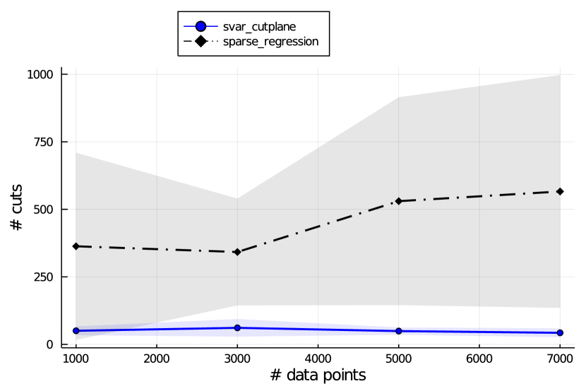
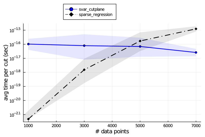
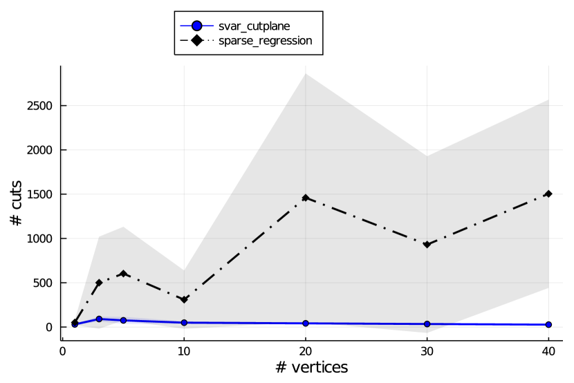
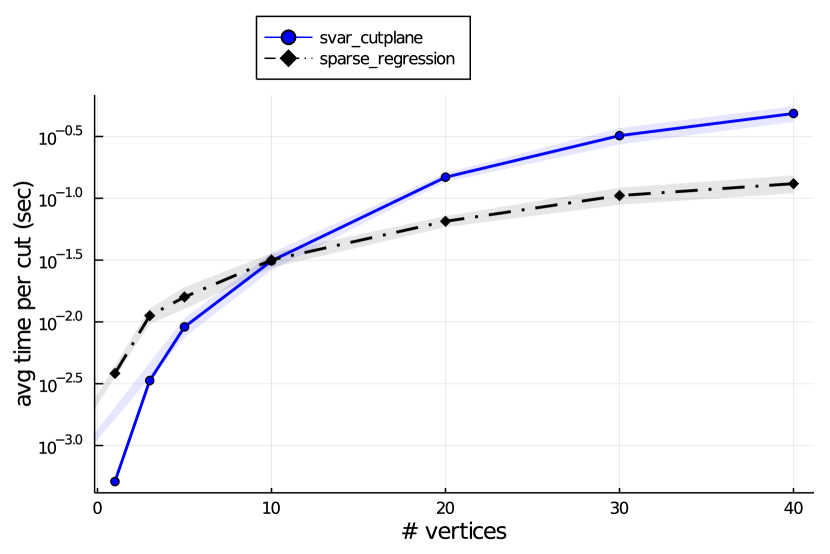
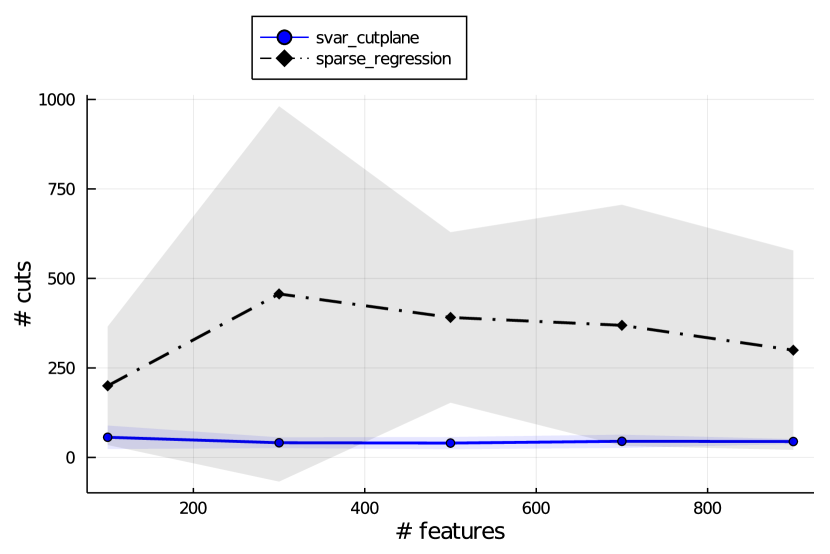
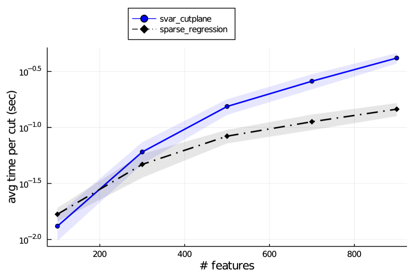
  (a) Number of cuts as function of N. (b) Average time per cut as function of N. (c) Number of cuts as function of T. (d) Average time per cut as function of T. (e) Number of cuts as function of D. (f) Average time per cut as function of D. Figure 3: Scalability of the cutting plane method with respect to $N,T,D$.

9 Experiments on Real-World Datasets

In this section, we study the performance of the SSVR framework on publicly available real-world data. We consider two datasets with temporally and three datasets with spatially varying structure. First, we present aggregated computational results; then, we delve deeper into each dataset and discuss the models learned by the proposed framework. In Appendix 14, we provide further information on the datasets and our preprocessing methodology, and detailed computational results.

Aggregated Results.

To obtain the aggregated results we report in this section, we randomly split each dataset 10 times into training ($60\%$), validation ($20\%$), and test ($20\%$) sets (respecting the temporal structure if such exists). For each dataset and each metric, we compute the mean and standard deviation of each method across those 10 splits. We rank the methods according to their performance and report the mean and standard deviation of the rank of each method across all experiments. Table 2 presents the aggregated results (obtained over $50$ datasets).

In agreement with our conclusions from Section 8, svar_cutplane, svar_hybrid, and sum_of_norms_l1 outperform in terms of their predictive power, with svar_cutplane and svar_hybrid having notably lower variance in their performance. As in real-world problems there is no way to assess estimation accuracy, we instead focus on model interpretability; we report each method’s estimated local sparsity ($\hat{K}_{\text{L}}$), global sparsity ($\hat{K}_{\text{G}}$), and number of changes in support $\hat{K}_{\text{C}}$. svar_cutplane, svar_hybrid, and svar_heuristic always produce simpler and hence more interpretable models using, in general, the smaller number of features. Similar to the synthetic experiments, svar_hybrid and svar_heuristic are the clear winners on computational time. Finally, the proposed methods significantly outperform static_cutplane on proving optimality and on generating fewer and faster cuts, i.e., on the evaluation of the cutting plane method.

Table 2: Aggregated results for real-world data: mean and std. of each method’s ranking across all experiments. Note that Gap, Cut Count, and ACT only apply to cutting plane-based methods.

Algorithm	Test R2	Local Sparsity	Global Sparsity	Changes in Support	Time	Gap	ACT	Cut Count
svar_cutplane	2.8 (0.84)	2.2 (1.3)	2.0 (1.22)	2.0 (1.41)	6.2 (1.48)	2.6 (3.05)	2.0 (0.0)	1.6 (0.89)
svar_hybrid	2.8 (0.45)	2.2 (2.17)	2.0 (1.73)	2.2 (1.79)	2.6 (0.89)	1.2 (0.45)	1.8 (1.1)	1.8 (0.45)
svar_heuristic	5.0 (1.58)	2.0 (1.73)	7.6 (0.89)	7.6 (0.89)	2.0 (1.41)	-	-	-
static_cutplane	6.6 (1.34)	3.6 (2.41)	2.4 (1.34)	1.0 (0.0)	6.2 (2.17)	2.4 (0.89)	2.2 (1.1)	2.6 (0.89)
sum_of_norms_l1	2.8 (2.95)	6.6 (0.89)	5.6 (0.89)	3.0 (1.41)	3.0 (1.22)	-	-	-
sum_of_norms_l1_lasso	6.4 (1.52)	4.0 (1.41)	3.4 (0.89)	5.6 (0.55)	3.2 (2.17)	-	-	-
sum_of_norms_l2	3.2 (2.68)	7.2 (0.45)	6.2 (0.45)	4.6 (2.07)	7.0 (0.71)	-	-	-
sum_of_norms_l2_lasso	5.2 (2.49)	5.2 (1.48)	4.8 (1.1)	6.8 (0.45)	5.6 (0.89)	-	-	-

9.1 Datasets with Temporally Varying Structure

In this section, we delve deeper into the temporal datasets and the corresponding learned models.

Appliances Energy Prediction: Hourly.

In this experiment, we focus on a real-world case study concerned with appliances energy prediction (Candanedo et al. 2017). Each observation in the dataset is a vector of measurements (temperature and humidity in various rooms, weather conditions, etc.) in a low energy building, and the goal is to predict the energy consumption of the building’s appliances. After preprocessing the dataset, we get $N=822$ data points per vertex, $T=24$ vertices (each corresponding to an hour of the day), and $D=26$ features; to capture the temporal structure of the problem, the similarity graph is a chain (see Figure 1 (left)); see Appendix 14.1 for details.

Our open-source implementation outputs the final model as a graph, with a structure matching that of the underlying similarity graph. Each vertex shows the learned regression coefficient for any selected feature at the corresponding vertex of the similarity graph; vertices in yellow (resp. blue) correspond to coefficients below (resp. above) the mean across all vertices.

Figure 4(a) presents the variation of the regression coefficient with the highest mean absolute magnitude across all vertices in the best svar_cutplane model. The corresponding feature, T4, corresponds to the temperature in the office room. $\bm{\beta}_{\text{T4}}$ is zero between 9pm and 10pm and, in general, takes very low values at night, when the office room is likely empty; then, it slowly increases during the day, peaks in the afternoon, and then slowly decreases in the evening. The slowly and sparsely varying structure of the learned model is clear.

Appliances Energy Prediction: Monthly.

In this experiment, we consider the same appliances energy dataset. However, instead of assigning a vertex to each hour of the day, we now assign a vertex to each month. We get $N=2,922$, $T=5$, $D=26$ and a chain similarity graph. Figure 4(b) presents the variation of the same regression coefficient across all vertices in the best svar_cutplane model. In this case, $\bm{\beta}_{\text{T4}}$ varies slowly across months, having a higher impact on the model as the summer approaches (when, potentially, the use of ACs increases consumption).

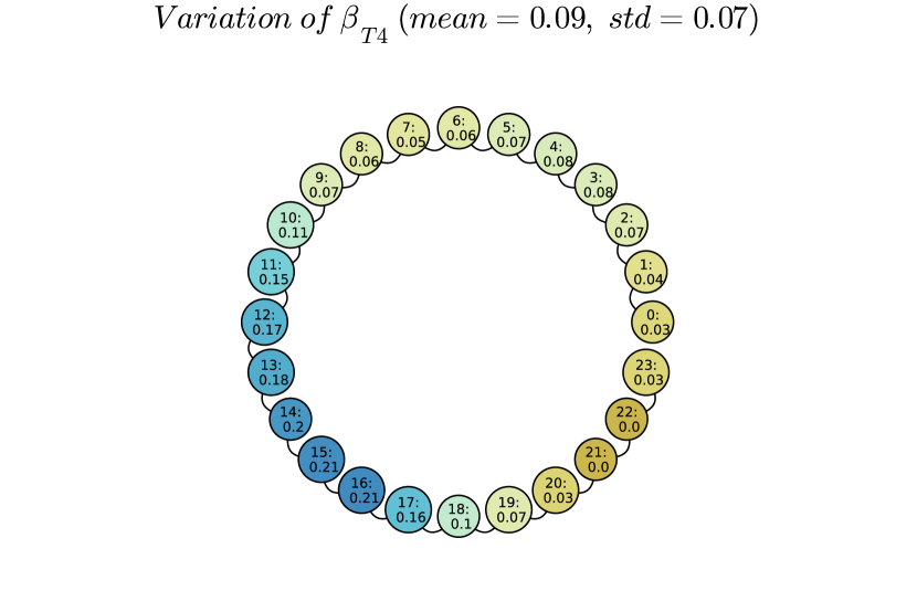
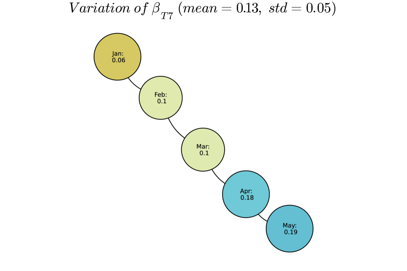
(a) Appliances Energy Prediction: Hourly. (b) Appliances Energy Prediction: Monthly. Figure 4: Variation of most important feature across vertices on datasets with temporally varying structure.

9.2 Datasets with Spatially Varying Structure

In this section, we discuss the details of the spatial datasets and the corresponding learned models.

Housing Price Prediction.

In this experiment, we explore the application of our framework to housing price prediction in Ames, Iowa (De Cock 2011). The dataset consists of a number of features involved in assessing home values, and the goal is to predict the selling price of the home. We get $N=822$, $T=7$ (each corresponding to a cluster of neighborhoods in Ames, Iowa; see Figure 5(a) for a visualization), $D=199$, and a similarity graph connecting adjacent neighborhood clusters with $E=8$ edges. Figure 5(b) presents the variation of the regression coefficient with the highest mean absolute magnitude across all vertices in the best svar_cutplane model. In this case, the corresponding feature, GrLivArea, corresponds to the above-ground living area. $\bm{\beta}_{\text{GrLivArea}}$ peaks in the northernmost neighborhood clusters and decreases in the southernmost clusters (W, S, E).

Air Quality.

In this experiment, we consider air quality prediction in 12 air quality monitoring sites in Beijing (Zhang et al. 2017). The original dataset consists of weather (temperature, pressure, dew point temperature, precipitation, wind speed, wind direction) and time-related features, and the goal is to predict PM2.5 concentration - an air pollutant that is a health concern at high levels. We get $N=35,064$, $T=12$ (each corresponding to an air quality monitoring site), $D=25$, and a similarity graph of $E=14$ edges and $4$ connected components. Figure 5(c) presents the variation of the regression coefficient with the highest mean absolute magnitude across all vertices in the best svar_cutplane model. In this case, the corresponding feature, DEWP, corresponds to the dew point temperature. The benefits of the proposed SSVR framework are again clear: the range of values for $\bm{\beta}_{\text{DEWP}}$ is between 0.38 and 0.48; however, across all connected components, the maximum coefficient variation never exceeds 0.01.

Meteorology.

In this experiment, we consider the task of weather prediction in 30 US and Canadian Cities, as well as 6 Israeli cities. The original dataset contains hourly measurements of weather attributes (temperature, humidity, air pressure, wind direction, and wind speed), and the goal is to predict the temperature half a day in advance. We get $N=45,231$, $T=36$ (each corresponding to a city), $D=50$ features, and a similarity graph of $E=110$ edges and $2$ connected components. Figure 5(d) presents the variation of the regression coefficient with the highest mean absolute magnitude across all vertices in the best svar_cutplane model. In this case, the corresponding feature, T1, corresponds, perhaps unsurprisingly, to the current temperature. The visualization of the learned model clearly shows how $\bm{\beta}_{\text{T1}}$ varies slowly across the similarity graph.

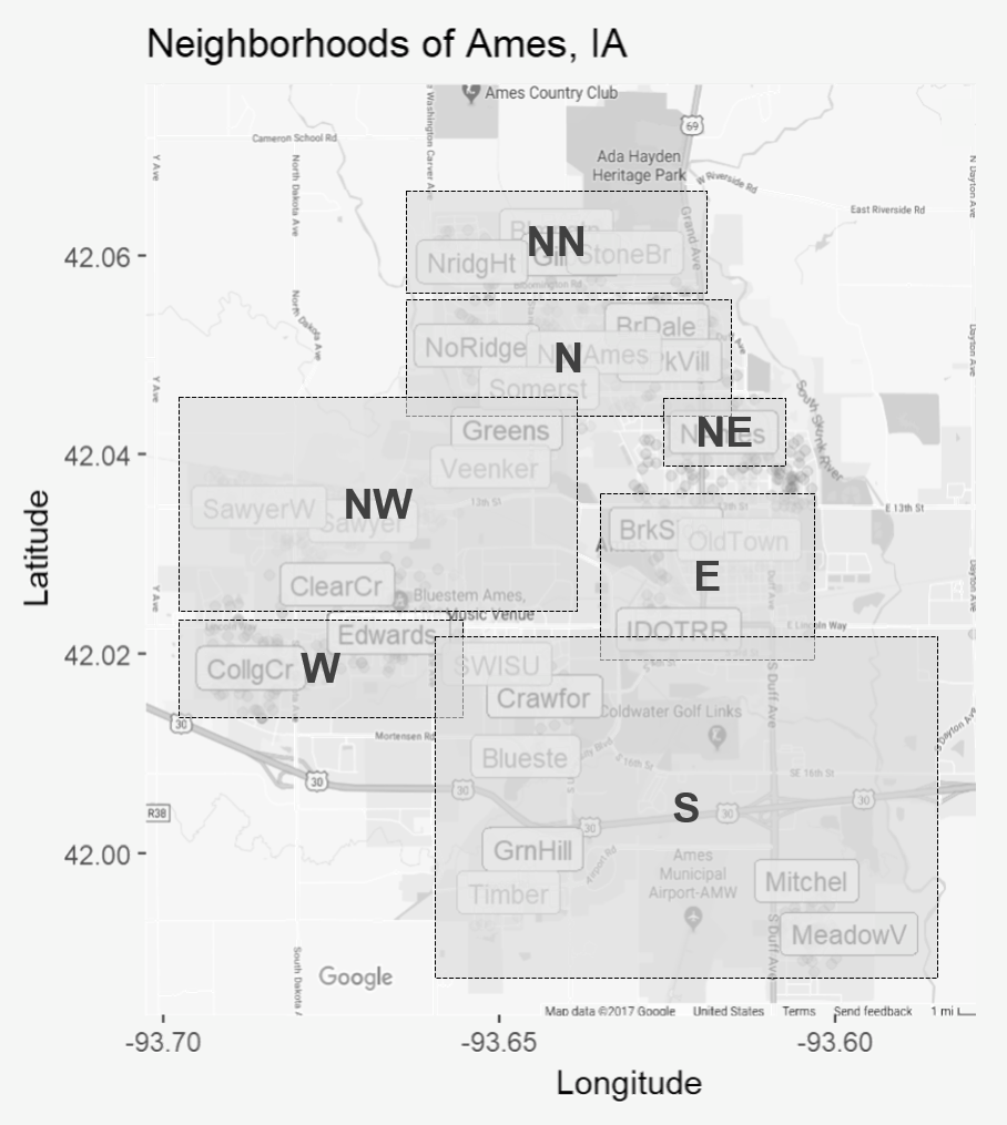
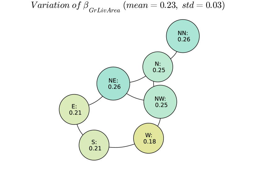
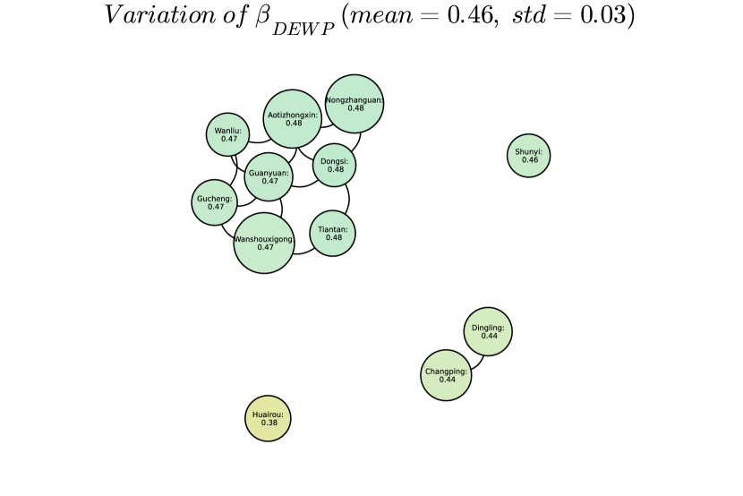
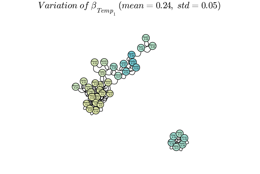
(a) Neighborhood clusters in Ames, IA. (b) Housing Price Prediction. (c) Air Quality. (d) Meteorology. Figure 5: Variation of most important feature across vertices on datasets with spatially varying structure.

10 Conclusion

In this paper, we have introduced the slowly varying regression under sparsity framework, which addresses regression problems with sparse and slowly varying structure. We have proposed a new way of solving the underlying optimization problem to optimality through a novel relaxation of the objective function. We have developed efficient exact and heuristic algorithms, as well as a practical hyperparameter tuning procedure, and have made our implementation available open-source to facilitate the use of the proposed framework by practitioners.

Our numerical experiments demonstrate the proposed methods’ superior or competitive performance in multiple dimensions—ranging from accuracy and interpretability to computational efficiency. Our results affirm the value proposition of our slowly varying methods, particularly svar_cutplane and svar_hybrid, in handling complex regression scenarios involving sparse and slowly varying coefficients. They offer a compelling blend of accuracy, computational efficiency, and interpretability, thereby establishing their potential for a wide range of applications in sparse regression problems. Future work could explore the integration of additional regularization techniques to further fine-tune these algorithms for specific use cases.

11 Technical Proofs

11.1 Proof of Lemma 1

Proof 11.1

Proof Note that by rearranging the variables, we can rewrite the optimization problem as:

$$\underset{\bm{z},\bm{s},\bm{w}\in\mathcal{Z}}{\min}\;\;\underset{\bm{\beta}}{\min}\quad c(\bm{z},\bm{\beta}):=\bm{\beta}^{\top}(\bm{Z}(\bm{M}+\lambda_{\beta}\bm{I})\bm{Z})\bm{\beta}-2\bm{\mu}^{\top}\bm{Z}\bm{\beta}+\sum_{t=1}^{T}\|\bm{y}^{t}\|_{2}^{2},$$

where $\bm{\beta}=(\bm{\beta}^{1},\cdots,\bm{\beta}^{T})$, $\bm{Z}=\operatorname{Diag}(\bm{z}^{1},\cdots,\bm{z}^{T})$, and $\mathcal{Z}$ is the polyhedral feasible set as defined by the binary constraints on $\bm{z},\bm{s},\bm{w}$ and (11)–(16), and $\bm{M}$ can be defined as:

$$\bm{M} =\begin{pmatrix}\bm{X}^{1}\\ \bm{X}^{2}\\ \vdots\\ \bm{X}^{T}\end{pmatrix}\begin{pmatrix}\bm{X}^{1}&\bm{X}^{2}&\dots&\bm{X}^{T}\end{pmatrix}+\begin{pmatrix}\mathbbm{1}_{\exists t,(1,t)\in E}-\mathbbm{1}_{\exists s,(s,1)\in E}\\ \mathbbm{1}_{\exists t,(2,t)\in E}-\mathbbm{1}_{\exists s,(s,2)\in E}\\ \vdots\\ \mathbbm{1}_{\exists t,(T,t)\in E}-\mathbbm{1}_{\exists s,(s,T)\in E}\end{pmatrix}\times\left(\begin{pmatrix}\mathbbm{1}_{\exists t,(1,t)\in E}-\mathbbm{1}_{\exists s,(s,1)\in E}\\ \mathbbm{1}_{\exists t,(2,t)\in E}-\mathbbm{1}_{\exists s,(s,2)\in E}\\ \vdots\\ \mathbbm{1}_{\exists t,(T,t)\in E}-\mathbbm{1}_{\exists s,(s,T)\in E}\end{pmatrix}\right)^{T}.$$

It is clear that the both matrices in the right expression are positive semidefinite, and thus $\bm{M}$ is positive semidefinite. We then reach the final form by dividing the objective by 2 and noting $\sum_{t=1}^{T}\|\bm{y}^{t}\|_{2}^{2}$ is a constant within the optimization problem and thus can be removed. $\square$

11.2 Proof of Lemma 2

Proof 11.2

Proof We first note that our minimization problem is equivalent to the sum-of-norms original problem. Combining this with the fact that $\bm{M}$ is positive semi-definite, to solve the inner problem we only need to derive the first order condition, which is:

$$\frac{\partial c(\bm{z},\bm{\beta})}{\partial\bm{\beta}}=(\bm{Z}(\bm{M}+\lambda_{\beta}\bm{I})\bm{Z})\bm{\beta}-\bm{Z}\bm{\mu}=\bm{0}.$$

$\bm{Z}$ is a rank $\leq TK_{\text{L}}<TD$ matrix, so $(\bm{Z}(\bm{M}+\lambda_{\beta}\bm{I})\bm{Z})$ is rank-deficient. Thus, to solve this first-order condition, we can utilize the Moore-Penrose pseudo-inverse to write $\bm{\beta}^{*}(\bm{z})=(\bm{Z}(\bm{M}+\lambda_{\beta}\bm{I})\bm{Z})^{\dagger}\bm{Z}\bm{\mu}.$

The second assertion follows from substituting the first order equality $(\bm{Z}(\bm{M}+\lambda_{\beta}\bm{I})\bm{Z})\bm{\beta}^{*}(\bm{z})=\bm{Z}\bm{\mu}$ into the objective expression. Noting that $\bm{Z}\bm{\beta}^{*}(\bm{z})=\bm{\beta}^{*}(\bm{z})$ by definition, we have $\frac{1}{2}\bm{\beta}^{*}(\bm{z})^{\top}(\bm{Z}(\bm{M}+\lambda_{\beta}\bm{I})\bm{Z})\bm{\beta}^{*}(\bm{z})-\bm{\mu}^{\top}\bm{Z}\bm{\beta}^{*}(\bm{z})=-\frac{1}{2}\bm{\beta}^{*}(\bm{z})^{\top}\bm{Z}\bm{\mu}=-\frac{1}{2}\bm{\beta}^{*}(\bm{z})^{\top}\bm{\mu}$. $\square$

11.3 Proof of Proposition 1

Proof 11.3

Proof We prove this in two steps. First, we establish the following relation for the pseudoinverse:

Lemma 3

$(\bm{Z}(\bm{M}+\lambda_{\beta}\bm{I})\bm{Z})^{\dagger}=(\lambda_{\beta}\bm{I}+\bm{Z}\bm{M}\bm{Z})^{-1}-\lambda_{\beta}(\bm{I}-\bm{Z}).$

Proof 11.4

Proof of Lemma 3 We verify that the expression on the right satisfies the definition of a Moore-Penrose pseudoinverse for $\bm{A}:=\bm{Z}(\bm{M}+\lambda_{\beta}\bm{I})\bm{Z}$. The Moore-Penrose pseudoinverse $\bm{A}^{\dagger}$ is the unique matrix that satisfies: 1. $\bm{A}^{\dagger}\bm{A}\bm{A}^{\dagger}=\bm{A}^{\dagger}$, 2. $\bm{A}\bm{A}^{\dagger}\bm{A}=\bm{A}$, 3. $(\bm{A}\bm{A}^{\dagger})^{*}=\bm{A}\bm{A}^{\dagger}$, 4. $(\bm{A}^{\dagger}\bm{A})^{*}=\bm{A}^{\dagger}\bm{A}$, where $*$ is the Hermitian operator with $\bm{A}^{*}_{ij}=\overline{\bm{A}_{ji}}$. The assertions follow immediately if we have $\bm{A}^{\dagger}\bm{A}=\bm{A}\bm{A}^{\dagger}=\bm{Z}$, which we next prove:

$$\bm{A}^{\dagger}\bm{A} =[(\lambda_{\beta}\bm{I}+\bm{Z}\bm{M}\bm{Z})^{-1}-\lambda_{\beta}(\bm{I}-\bm{Z})]\bm{Z}(\bm{M}+\lambda_{\beta}\bm{I})\bm{Z}$$

$$=(\lambda_{\beta}\bm{I}+\bm{Z}\bm{M}\bm{Z})^{-1}(\bm{Z}\bm{M}\bm{Z}+\lambda_{\beta}\bm{Z})$$

$$=(\bm{I}-(\lambda_{\beta}\bm{I}+\bm{Z}\bm{M}\bm{Z})^{-1}\lambda_{\beta}(\bm{I}-\bm{Z}))$$

$$=(\bm{I}-\left(\frac{1}{\lambda_{\beta}}(\bm{I}-\bm{Z}(\lambda_{\beta}\bm{I}+\bm{M}\bm{Z})^{-1}\bm{M}\bm{Z})\right)\lambda_{\beta}(\bm{I}-\bm{Z}))$$

$$=\bm{Z},$$

where on the second last line we utilized the binomial inverse theorem (Henderson and Searle 1981). Here, we have $\bm{Z}^{2}=\bm{Z}$ as $\bm{Z}$ is a binary diagonal matrix. The case for $\bm{A}\bm{A}^{\dagger}$ is identical. $\square$

Then, we note the following equivalence:

Lemma 4

$(\lambda_{\beta}\bm{I}+\bm{Z}\bm{M}\bm{Z})^{-1}\bm{Z}=(\lambda_{\beta}\bm{I}+\bm{Z}\bm{M})^{-1}\bm{Z}.$

Proof 11.5

Proof of Lemma 4 By the binomial inverse theorem (Henderson and Searle 1981), we have:

$$(\lambda_{\beta}\bm{I}+\bm{Z}\bm{M}\bm{Z})^{-1}\bm{Z}=\frac{1}{\lambda_{\beta}}(\bm{I}-\bm{Z}(\lambda_{\beta}\bm{I}+\bm{M}\bm{Z})^{-1}\bm{M}\bm{Z})\bm{Z}=\frac{1}{\lambda_{\beta}}(\bm{Z}-\bm{Z}(\lambda_{\beta}\bm{I}+\bm{M}\bm{Z})^{-1}\bm{M}\bm{Z}).$$

Similarly, we have:

$$(\lambda_{\beta}\bm{I}+\bm{Z}\bm{M})^{-1}\bm{Z}=\frac{1}{\lambda_{\beta}}(\bm{I}-\bm{Z}(\lambda_{\beta}\bm{I}+\bm{M}\bm{Z})^{-1}\bm{M})\bm{Z}=\frac{1}{\lambda_{\beta}}(\bm{Z}-\bm{Z}(\lambda_{\beta}\bm{I}+\bm{M}\bm{Z})^{-1}\bm{M}\bm{Z}).$$

This proves the statement required. $\square$

We now prove the final desired statement, utilizing Lemmata 3 and 4:

$$(\bm{Z}(\bm{M}+\lambda_{\beta}\bm{I})\bm{Z})^{\dagger}\bm{Z}=((\lambda_{\beta}\bm{I}+\bm{Z}\bm{M}\bm{Z})^{-1}-\lambda_{\beta}(\bm{I}-\bm{Z}))\bm{Z}=(\lambda_{\beta}\bm{I}+\bm{Z}\bm{M})^{-1}\bm{Z}.$$

$\square$

11.4 Proof of Theorem 1

Proof 11.6

Proof The equivalence of the two optimization problems follows immediately from Lemma 2 and Proposition 1. We proceed to prove that $f(\bm{z})=-\frac{\bm{\mu}^{\top}\bm{\beta}^{*}(\bm{z})}{2}$ is convex in $\bm{z}$. Now, denote the element-wise products $(\bm{\beta}\cdot\bm{M})_{ij}=\beta_{i}M_{ij}$ and $(\bm{\beta}\cdot\bm{\mu})=\beta_{i}\mu_{i}$. Then, by direct calculation, the Hessian of $f(\bm{z})$ in the direction of $\bm{\beta}$ can be calculated as:

$$\bm{\beta}^{\top}\frac{\partial f(\bm{z})}{\partial\bm{z}\partial\bm{z}^{\top}}\bm{\beta}$$

$$=\bm{\mu}^{\top}(\lambda_{\beta}\bm{I}+\bm{Z}\bm{M})^{-1}(\bm{\beta}\cdot\bm{M})(\lambda_{\beta}\bm{I}+\bm{Z}\bm{M})^{-1}(\bm{\mu}\cdot\bm{\beta})$$

$$-\bm{\mu}^{\top}(\lambda_{\beta}\bm{I}+\bm{Z}\bm{M})^{-1}(\bm{\beta}\cdot\bm{M})(\lambda_{\beta}\bm{I}+\bm{Z}\bm{M})^{-1}((\bm{\beta}\cdot\bm{M})(\lambda_{\beta}\bm{I}+\bm{Z}\bm{M})^{-1}\bm{Z}\bm{\mu})$$

$$=\bm{\mu}^{\top}(\lambda_{\beta}\bm{I}+\bm{Z}\bm{M})^{-1}(\bm{\beta}\cdot\bm{M})(\lambda_{\beta}\bm{I}+\bm{Z}\bm{M})^{-1}(\bm{\beta}\cdot(\bm{I}-\bm{M}(\lambda_{\beta}\bm{I}+\bm{Z}\bm{M})^{-1}\bm{Z})\bm{\mu})$$

$$=\frac{1}{\lambda_{\beta}}\bm{\mu}^{\top}(\lambda_{\beta}\bm{I}+\bm{Z}\bm{M})^{-1}(\bm{\beta}\cdot\bm{M})(\lambda_{\beta}\bm{I}+\bm{Z}\bm{M})^{-1}(\bm{\beta}\cdot(\lambda_{\beta}\bm{I}+\bm{M}\bm{Z})^{-1}\bm{\mu})$$

$$=\frac{1}{\lambda_{\beta}}(\bm{\beta}\cdot(\lambda_{\beta}\bm{I}+\bm{M}\bm{Z})^{-1}\bm{\mu})^{\top}\bm{M}(\bm{I}+\bm{Z}\bm{M})^{-1}(\bm{\beta}\cdot(\lambda_{\beta}\bm{I}+\bm{M}\bm{Z})^{-1}\bm{\mu})$$

$$=\frac{1}{\lambda_{\beta}}(\bm{\beta}\cdot(\lambda_{\beta}\bm{I}+\bm{M}\bm{Z})^{-1}\bm{\mu})^{\top}\bm{M}(\bm{M}+\bm{M}\bm{Z}\bm{M})^{\dagger}\bm{M}(\bm{\beta}\cdot(\lambda_{\beta}\bm{I}+\bm{M}\bm{Z})^{-1}\bm{\mu})$$

$$\geq 0,$$

where, in the second last step, we utilized:

$$\bm{M}(\bm{I}+\bm{Z}\bm{M})^{-1}=\bm{M}\bm{M}^{\dagger}\bm{M}(\bm{I}+\bm{Z}\bm{M})^{-1}=\bm{M}\bm{M}^{\dagger}(\bm{I}+\bm{M}\bm{Z})^{-1}\bm{M}=\bm{M}(\bm{M}+\bm{M}\bm{Z}\bm{M})^{\dagger}\bm{M}.$$

Since $\bm{M},\bm{Z}$ are both positive semi-definite, it is clear that $(\bm{M}+\bm{M}\bm{Z}\bm{M})^{\dagger}$ is positive semi-definite, and thus the Hessian of $f(\bm{z})$ in the direction of $\bm{\beta}$ is always non-negative. Since this inequality holds for any $\bm{\beta}$, the Hessian matrix of $f(\bm{z})$ is positive semidefinite and hence $f(\bm{z})$ is convex in $\bm{z}$. $\square$

11.5 Proof of Lemma 3

Proof 11.7

Proof We begin by differentiating matrix $\bm{K}$ with respect to $\bm{Z}$’s diagonal component $z^{t}_{d}$:

$$\begin{split}\frac{\partial\bm{K}}{\partial z^{t}_{d}}=\frac{\partial\bm{K}(\bm{z})}{\partial z^{t}_{d}}=\frac{\partial\left(\lambda_{\beta}\mathbb{I}+\bm{Z}\bm{M}\right)}{\partial z^{t}_{d}}=\bm{E^{t}_{d}}\bm{M}.\end{split}$$ (24)

The partial derivative of the inverse of $\bm{K}$ is then given by

$$\begin{split}\frac{\partial\bm{K}^{-1}}{\partial z^{t}_{d}}=-\bm{K}^{-1}\frac{\partial\bm{K}}{\partial z^{t}_{d}}\bm{K}^{-1}=-\bm{K}^{-1}\bm{E^{t}_{d}}\bm{M}\bm{K}^{-1}.\end{split}$$ (25)

Finally, we have

$$\frac{\partial c(\bm{z})}{\partial z^{t}_{d}}=\frac{\partial\left(-\frac{1}{2}\bm{\mu}^{\top}\bm{K}^{-1}\bm{Z}\bm{\mu}\right)}{\partial z^{t}_{d}}=\frac{1}{2}\bm{\mu}^{\top}\bm{K}^{-1}\left(\bm{E^{t}_{d}}\bm{M}\bm{K}^{-1}\bm{Z}\ -\ \bm{E^{t}_{d}}\right)\bm{\mu}.$$ (26)

$\square$

11.6 Proof of Lemma 4

Proof 11.8

Proof We first introduce some notation: given any vector (matrix) $\bm{a}$ ($\bm{A}$) and a binary vector $\bm{z}$ (feasible for Problem (19)), $\bm{a}_{\bm{z}}$ ($\bm{A}_{\bm{z},:}$ or $\bm{A}_{:,\bm{z}}$) is formed by selecting all entries $(t,d)$ of vector $\bm{a}$ (all rows $(t,d)$ or all columns $(t,d)$ of matrix $\bm{A}$, respectively) for which $z_{d}^{t}=1$. Accordingly, the subscript $\bm{z}^{c}$ selects the entries/rows/columns for which $z_{d}^{t}=0$.

Cost function evaluation.

Define $\bm{K}=(\lambda_{\beta}\bm{I}+\bm{Z}\bm{M})$. Then, given a feasible binary vector $\bm{z}$, the cost function $c(\bm{z})$ is $-\frac{1}{2}\bm{\mu}^{\top}\bm{K}^{-1}\bm{Z}\bm{\mu}$. To evaluate this equation, we first need to invert matrix $\bm{K}$. The size of matrix $\bm{K}$ is $TD\times TD$, so a naive implementation would require $O\left(T^{3}D^{3}\right)$ operations. We can reduce the complexity of the inversion by exploiting the structure of the matrix as follows:

• We reorder the rows and columns of matrix $\bm{K}$ so that it takes the form:

  $$\bm{\tilde{K}}:=\left[\begin{array}[]{cc}\lambda_{\beta}\bm{I}+\bm{M}_{\bm{z},\bm{z}}&\bm{M}_{\bm{z},\bm{z}^{c}}\\ \bm{0}&\lambda_{\beta}\bm{I}\end{array}\right],$$

  where $\bm{M}_{\bm{z},\bm{z}}\in\mathbb{R}^{TK_{\text{L}}\times TK_{\text{L}}}$ and $\bm{M}_{\bm{z},\bm{z}^{c}}\in\mathbb{R}^{TK_{\text{L}}\times T(D-K_{\text{L}})}$. We then similarly reorder $\bm{\mu}$ and $\bm{Z}$ to $\bm{\tilde{\mu}}=[\bm{\mu}_{\bm{z}},\bm{\mu}_{\bm{z}^{c}}]$ and $\bm{\tilde{Z}}=\operatorname{Diag}(\bm{1}_{\bm{z}},\bm{0}_{\bm{z}^{c}})$. Note that the reordering does not change the objective value, and therefore the objective function is now $-\frac{1}{2}\bm{\tilde{\mu}}^{\top}\bm{\tilde{K}}^{-1}\bm{\tilde{Z}}\bm{\tilde{\mu}}.$

• We perform blockwise inversion, which gives

  $$\bm{\tilde{K}}^{-1}=\begin{bmatrix}(\lambda_{\beta}\bm{I}+\bm{M}_{\bm{z},\bm{z}})^{-1}&\frac{1}{\lambda_{\beta}}(\lambda_{\beta}\bm{I}+\bm{M}_{\bm{z},\bm{z}})^{-1}\bm{M}_{\bm{z},\bm{z}^{c}}\\ \bm{0}&\frac{1}{\lambda_{\beta}}\bm{I}\end{bmatrix}.$$ (27)

  Since $\bm{Z}$ has zeros on the diagonals for all $\bm{z}^{c}$ columns, we thus have

  $$\bm{\tilde{K}}^{-1}\bm{\tilde{Z}}=\begin{bmatrix}(\lambda_{\beta}\bm{I}+\bm{M}_{\bm{z},\bm{z}})^{-1}&\bm{0}\\ \bm{0}&\bm{0}\end{bmatrix}$$ (28)

  and therefore the objective function can be now written as $-\frac{1}{2}\bm{\tilde{\mu}}^{\top}\bm{\tilde{K}}^{-1}\bm{\tilde{Z}}\bm{\tilde{\mu}}=-\frac{1}{2}\bm{\mu}^{\top}_{\bm{z}}(\lambda_{\beta}\bm{I}+\bm{M}_{\bm{z},\bm{z}})^{-1}\bm{\mu}_{\bm{z}}.$ Noting that the matrix $(\lambda_{\beta}\bm{I}+\bm{M}_{\bm{z},\bm{z}})$ has block tri-diagonal structure, with $T$ blocks of size $K_{\text{L}}\times K_{\text{L}}$ each, its inverse $(\lambda_{\beta}\bm{I}+\bm{M}_{\bm{z},\bm{z}})^{-1}$ can be computed by recursive application of blockwise inversion in $O\left(T^{2}K_{\text{L}}^{2}(T+K_{\text{L}})\right)$ operations.

• The remaining operations to evaluate the objective are the vector-matrix multiplications with $\bm{\mu}_{\bm{z}}$, which require $O(T^{2}K_{L}^{2})$ operations.

Gradient evaluation.

We compute each of the $TD$ gradient entries as per Lemma 3: $\frac{\partial c(\bm{z})}{\partial z^{t}_{d}}=\frac{1}{2}\bm{\mu}^{\top}\bm{K}^{-1}\left(\bm{E^{t}_{d}}\bm{M}\bm{K}^{-1}\bm{Z}\ -\ \bm{E^{t}_{d}}\right)\bm{\mu}.$ $\bm{v}^{i}\in\mathbb{R}^{TD}$ denotes auxiliary vectors, and we work as follows:

• We compute $\bm{K}^{-1}\bm{Z}\bm{\mu}$. Noting that $\bm{K}^{-1}\bm{Z}$ selects the columns $(t,d)$ of $\bm{K}^{-1}$ for which $z_{d}^{t}=1$ and sets the remaining columns to $0$, and observing that $\bm{K}^{-1}_{\bm{z}^{c},\bm{z}}=\bm{0}$ from Equation 27, we in fact only need to compute $\bm{v^{0}}_{\bm{z}}=\bm{K}^{-1}_{\bm{z},\bm{z}}\bm{\mu}_{\bm{z}}.$ The remaining entries of $\bm{v^{0}}\in\mathbb{R}^{TD}$, i.e., $\bm{v^{0}}_{\bm{z}^{c}}$, are set to $0$. This only needs to be performed once independent of which gradient entry is being computed, and we have $\bm{K}^{-1}$ from the evaluation of the cost function. Thus, the complexity is $O\left(T^{2}K_{\text{L}}^{2}\right)$ operations.

• We compute $\bm{\mu}^{\top}\bm{K}^{-1}$, namely, $\bm{v^{1}}_{\bm{z}}=\left(\bm{\mu}^{\top}_{\bm{z}}\bm{K}^{-1}_{\bm{z},\bm{z}}\right)^{\top},$ which requires $O\left(T^{2}K_{\text{L}}^{2}\right)$ operations. To compute the remaining entries of $\bm{v^{1}}\in\mathbb{R}^{TD}$, i.e., $\bm{v^{1}}_{\bm{z}^{c}}$, we again reorder $\bm{\mu}$ to be $\bm{\tilde{\mu}}:=[\bm{\mu}_{\bm{z}},\bm{\mu}_{\bm{z}^{c}}]$ similar to above, and then use the formula indicated in Equation (27). Put together, we have

  $$\bm{v^{1}} =\begin{bmatrix}\bm{\mu}_{\bm{z}}^{\top}(\lambda_{\beta}\bm{I}+\bm{M}_{\bm{z},\bm{z}})^{-1}&\quad\frac{1}{\lambda_{\beta}}\left(\bm{\mu}_{\bm{z}}^{\top}(\lambda_{\beta}\bm{I}+\bm{M}_{\bm{z},\bm{z}})^{-1}\bm{M}_{\bm{z},\bm{z}^{c}}+\bm{\mu}_{\bm{z}^{c}}^{\top}\right)\end{bmatrix}$$

  $$=\begin{bmatrix}\bm{v^{1}}_{\bm{z}}&\quad\frac{1}{\lambda_{\beta}}\left(\bm{v^{1}}_{\bm{z}}\bm{M}_{\bm{z},\bm{z}^{c}}+\bm{\mu}_{\bm{z}^{c}}^{\top}\right)\end{bmatrix},$$ (29)

  which requires $O\left(T^{2}K_{\text{L}}D\right)$ operations. The above steps only need to be performed once, independently of which entry of the gradient is being computed. Overall, the complexity is $O\left(T^{2}K_{\text{L}}D\right)$ operations.

• For each $(t,d)$, we compute the multiplication $\left(\bm{E^{t}_{d}}\bm{M}\right)\left(\bm{K}^{-1}\bm{Z}\bm{\mu}\right)$. Noting that the multiplication $\bm{E^{t}_{d}}\bm{M}$ yields a matrix that is nonzero only at row $(t,d)$, and since the result is multiplied with the vector $\bm{K}^{-1}\bm{Z}\bm{\mu}$, we implement the multiplication as $\bm{v^{2}}_{(t,d)}=\bm{M}_{(t,d),\bm{z}}\bm{v^{0}}_{\bm{z}}.$ This requires $O\left(T^{2}DK_{\text{L}}\right)$ operations in total across all $(t,d)$.

• For each $(t,d)$, we compute the multiplication $\left(\bm{\mu}^{\top}\bm{K}^{-1}\right)\left(\bm{E^{t}_{d}}\bm{M}\bm{K}^{-1}\bm{Z}\bm{\mu}\right)$. We first note that $\bm{E^{t}_{d}}=\bm{E^{t}_{d}}\bm{E^{t}_{d}}$ and hence the multiplication can be rewritten as: $\left(\bm{\mu}^{\top}\bm{K}^{-1}\bm{E^{t}_{d}}\right)\left(\bm{E^{t}_{d}}\bm{M}\bm{K}^{-1}\bm{Z}\bm{\mu}\right)=\left(\bm{\mu}^{\top}\bm{K}^{-1}\bm{E^{t}_{d}}\right)\left(\bm{E^{t}_{d}}\bm{v}^{2}\right)$. Therefore, the first term selects the $(t,d)$ column of $\bm{\mu}^{\top}\bm{K}^{-1}$ and the second term selects the $(t,d)$ row of $\bm{v}^{2}$. Using this fact, along with Equation (• ‣ 11.6), we can now go back and calculate the final product $\bm{v^{3}}_{(t,d)}=\left(\bm{\mu}^{\top}\bm{K}^{-1}\bm{E^{t}_{d}}\right)\left(\bm{E^{t}_{d}}\bm{M}\bm{K}^{-1}\bm{Z}\bm{\mu}\right)=\bm{v^{1}}_{(t,d)}\cdot\bm{v^{2}}_{(t,d)}.$ The complexity is $O\left(TD\right)$ operations in total across all $(t,d)$.

• For each $(t,d)$, we compute the multiplication $\bm{\mu}^{\top}\bm{K}^{-1}\bm{E^{t}_{d}}\bm{\mu}$ as $\bm{v^{4}}_{(t,d)}=\bm{v^{1}}_{(t,d)}\cdot\bm{\mu}_{(t,d)}+\mathbbm{1}_{\left(z^{t}_{d}=0\right)}\frac{(\bm{\mu}_{(t,d)})^{2}}{\lambda_{\beta}}.$ This requires $O\left(TD\right)$ operations in total across all $(t,d)$.

• For each $(t,d)$, we compute ($O\left(TD\right)$ operations in total across all $(t,d)$) the corresponding entry of the gradient as $\frac{\partial c(\bm{z})}{\partial z^{t}_{d}}=\frac{\bm{v^{3}}_{(t,d)}-\bm{v^{4}}_{(t,d)}}{2}.$

After completing the steps outlined above, we have the ingredients to compute all entries of the gradient $\nabla_{\bm{z}}c(\bm{z})$. In total, the cost is $O\left(T^{2}DK_{\text{L}}\right)$ operations.

Cut generation.

The complexity of the entire process is $O\left(T^{2}K_{\text{L}}[K_{\text{L}}(T+K_{\text{L}})+D]\right).$ $\square$

11.7 Proof of Lemma 5

Proof 11.9

Proof Let us denote by $\mathcal{Z}_{\beta}$ the feasible set defined by Equations (2)-(4). We upper bound Problem (1)-(4) as follows:

$$\underset{\bm{\beta}\in\mathcal{Z}_{\beta}}{\min}\quad\sum_{n=1}^{N}\sum_{t=1}^{T}\left(y_{n}^{t}-\sum_{d=1}^{D}X_{n,d}^{t}\beta_{d}^{t}\right)^{2}+\lambda_{\beta}\sum_{t=1}^{T}\sum_{d=1}^{D}\left(\beta_{d}^{t}\right)^{2}+\lambda_{\delta}\sum_{(s,t)\in E}\sum_{d=1}^{D}\left(\beta_{d}^{t}-\beta_{d}^{s}\right)^{2}$$ (30)

$$\leq\frac{1}{D}\sum_{d=1}^{D}\quad\underset{\bm{\beta}_{d}}{\min}\quad\sum_{n=1}^{N}\sum_{t=1}^{T}\left(y_{n}^{t}-X_{n,d}^{t}\beta_{d}^{t}\right)^{2}+\lambda_{\beta}\sum_{t=1}^{T}\left(\beta_{d}^{t}\right)^{2}+\lambda_{\delta}\sum_{(s,t)\in E}\left(\beta_{d}^{t}-\beta_{d}^{s}\right)^{2}$$ (31)

$$=\underset{\bm{\beta}}{\min}\quad\frac{1}{D}\sum_{d=1}^{D}\left(\sum_{n=1}^{N}\sum_{t=1}^{T}\left(y_{n}^{t}-X_{n,d}^{t}\beta_{d}^{t}\right)^{2}+\lambda_{\beta}\sum_{t=1}^{T}\left(\beta_{d}^{t}\right)^{2}+\lambda_{\delta}\sum_{(s,t)\in E}\left(\beta_{d}^{t}-\beta_{d}^{s}\right)^{2}\right)$$ (32)

$$\leq\underset{\bm{\beta}\in\mathcal{Z}_{\beta}}{\min}\quad\frac{1}{D}\sum_{n=1}^{N}\sum_{t=1}^{T}\sum_{d=1}^{D}\left(y_{n}^{t}-X_{n,d}^{t}\beta_{d}^{t}\right)^{2}+\lambda_{\beta}\sum_{t=1}^{T}\sum_{d=1}^{D}\left(\beta_{d}^{t}\right)^{2}+\lambda_{\delta}\sum_{(s,t)\in E}\sum_{d=1}^{D}\left(\beta_{d}^{t}-\beta_{d}^{s}\right)^{2}$$ (33)

$$\leq\underset{\bm{\beta}\in\mathcal{Z}_{\beta}}{\min}\quad\frac{1}{D}\sum_{n=1}^{N}\sum_{t=1}^{T}\sum_{d=1}^{D}\left(y_{n}^{t}-X_{n,d}^{t}\beta_{d}^{t}\right)^{2}+\lambda_{\beta}\sum_{t=1}^{T}\sum_{d=1}^{D}\left(\beta_{d}^{t}\right)^{2}+\lambda_{\delta}\sum_{(s,t)\in E}\sum_{d=1}^{D}2[\left(\beta_{d}^{t}\right)^{2}+\left(\beta_{d}^{s}\right)^{2}]$$ (34)

$$=\underset{\bm{\beta}\in\mathcal{Z}_{\beta}}{\min}\quad\frac{1}{D}\sum_{n=1}^{N}\sum_{t=1}^{T}\sum_{d=1}^{D}\left(y_{n}^{t}-X_{n,d}^{t}\beta_{d}^{t}\right)^{2}+\lambda_{\beta}\sum_{t=1}^{T}\sum_{d=1}^{D}\left(\beta_{d}^{t}\right)^{2}+\lambda_{\delta}\sum_{t=1}^{T}\sum_{d=1}^{D}2d^{t}\left(\beta_{d}^{t}\right)^{2}.$$ (35)

For the first inequality, in (30) we have the prediction error of the best multivariate model, which by definition is less than or equal to the error of any univariate model. This can therefore be upper bounded by the average error among all univariate models, which is what we have in (31). Observe that the best among these univariate models is indeed feasible for the minimization problem in (30). The equality between (31) and 32 is due to separability. For the second inequality, in 32 we have an unconstrained problem, whereas, in 33 we require that $\bm{\beta}\in\mathcal{Z}_{\beta}$ hence restricting the feasible set. Moreover, in 33 we rescale the regularization term and the slowly varying penalty with $D$ so that their relative importance compared to the prediction error is in the same order as in the original problem. For the third inequality, we trivially bound the squares of the differences between coefficients in adjacent vertices. $\square$

11.8 Proof of Proposition 2

Proof 11.10

Proof The termination condition of Algorithm 2 guarantees that, at termination, the solution must be a feasible solution for Problem (1)-(4). Therefore, we only need to prove that Algorithm 2 terminates in polynomial time, which we do step-by-step.

Algorithm 2’s first step computes the loss for each vertex-feature pair. This requires solving $TD$ univariate regularized least squares problems and can be done in closed form in time $O(NTD)$.

The second step involves solving a linear optimization problem over $TD$ variables. This can be done in time $\tilde{O}((TD)^{2+\nicefrac{{1}}{{6}}})$ using the algorithm by Cohen et al. (2021). (We note that $\tilde{O}(\cdot)$ gives the asymptotic complexity ignoring logarithmic factors.)

The third step involves ensuring integrality by iterating over all entries of the linear optimization problem’s solution, and can be done in time $O(TD)$.

The fourth step involves ensuring feasibility by removing one feature at a time as long as the linear optimization problem’s solution is infeasible. Let us denote by $S$ the global support (across all vertices) of the estimated regression coefficients. Since, after each iteration, we remove one feature from $S$, the global sparsity constraint (3) is guaranteed to be satisfied after at most $D-K_{\text{G}}$ iterations. Similarly, after at most $D-(K_{\text{L}}+\frac{K_{\text{C}}}{2})$ iterations, all vertices will be constrained to include the same set of $K_{\text{L}}+\frac{K_{\text{C}}}{2}$ features and hence any pair of similar regressions will differ in at most $K_{\text{C}}$ features. Therefore, the while loop terminates in at most

$$\max\{D-K_{\text{G}},D-(K_{\text{L}}+\frac{K_{\text{C}}}{2})\}$$

iterations, which gives an asymptotic complexity of $O(D).$ The complexity of each iteration is $O(T)$: in an efficient implementation, the first two steps inside the while loop are performed once, and, in each iteration, we only update the corresponding data structures in $O(1)$ time. Therefore, the fourth step can be done in time $O(TD).$

The fifth step involves computing $\tilde{\bm{\beta}}$ for the estimated support $\tilde{\bm{z}}$. This can be done in time $O(T^{2}K_{\text{L}}^{2}(T+K_{\text{L}}))$ using the procedure described in the proof of Lemma 4.

Thus, Algorithm 2 terminates in polynomial time with a feasible solution to Problem (1)-(4). $\square$

11.9 Proof of Proposition 2

We first prove the result for Algorithm 1 with validation cost function $c_{V}^{*}$. For any parameter set $(K_{L},K_{G},K_{C})$, as the number of training samples $N\to\infty$, the squared loss $\sum_{t=1}^{T}\left\|\bm{y}^{t}-\bm{X}^{t}\bm{\beta}^{t}\right\|_{2}^{2}$ within Equation (1) becomes the dominant term as it is the only term that scales with $N$. For any parameter set $(K_{L},K_{G},K_{C})$ with $K_{L}\geq K_{L}^{*},K_{G}\geq K_{G}^{*},\text{ and }K_{C}\geq K_{C}^{*}$, as number of training samples $N\to\infty$, the minimizer $\bm{\beta}^{*}(\bm{\lambda})\to\bm{\beta}^{0}$ by standard asymptotic theory of linear regression. (e.g., DasGupta 2008) Therefore, as $N\to\infty$, the validation cost on $N_{V}$ samples tend to:

$$c_{V}^{*}(\bm{\lambda})\quad\to\quad N_{V}\sum_{t=1}^{T}(\epsilon_{n}^{t})^{2}+\lambda_{\beta}\sum_{t=1}^{T}\|\bm{\beta}^{0^{t}}\|_{2}^{2}+\lambda_{\delta}\sum_{(s,t)\in E}\|\bm{\beta}^{0^{t}}-\bm{\beta}^{0^{s}}\|_{2}^{2}.$$

Alternatively, for any parameter set $(K_{L},K_{G},K_{C})$ with $K_{L}<K_{L}^{*}$, $K_{G}<K_{G}^{*}$, or $K_{C}<K_{C}^{*}$, as number of training samples $N\to\infty$, the minimizer $\bm{\beta}^{*}(\bm{\lambda})\to\tilde{\bm{\beta}}\neq\bm{\beta}^{0}$ as $\bm{\beta}^{0}$ is infeasible. Therefore, as $N\to\infty$, the validation cost on $N_{V}$ samples tend to:

$$c_{V}^{*}(\bm{\lambda})\quad\to\quad\sum_{t=1}^{T}\|\bm{y}^{t}-\bm{X}^{t}\tilde{\bm{\beta}}^{t}\|^{2}+\lambda_{\beta}\sum_{t=1}^{T}\|\tilde{\bm{\beta}}^{t}\|_{2}^{2}+\lambda_{\delta}\sum_{(s,t)\in E}\|\tilde{\bm{\beta}}^{t}-\tilde{\bm{\beta}}^{s}\|_{2}^{2}.$$

Now, by construction, $\bm{\beta}^{0}$ is the unique optimal solution of the linear regression problem:

$$\min_{\bm{\beta}^{t}}\sum_{t=1}^{T}\mathbb{E}[\left\|y_{n}^{t}-\bm{x}_{n}^{t}\bm{\beta}^{t}\right\|_{2}^{2}]=\sum_{t=1}^{T}\mathbb{E}[(\epsilon_{n}^{t})^{2}].$$

Thus, since $\tilde{\bm{\beta}}\neq\bm{\beta}^{0}$, we have that, as $N_{V}\to\infty$:

$$\frac{\sum_{t=1}^{T}\|\bm{y}^{t}-\bm{X}^{t}\tilde{\bm{\beta}}^{t}\|^{2}}{N_{V}}\to\sum_{t=1}^{T}\mathbb{E}[\|y_{n}^{t}-\bm{x}_{n}^{t}\tilde{\bm{\beta}}^{t}\|^{2}]>\sum_{t=1}^{T}\mathbb{E}[(\epsilon_{n}^{t})^{2}].$$

In particular, we have that:

$$\sum_{t=1}^{T}\|\bm{y}^{t}-\bm{X}^{t}\tilde{\bm{\beta}}^{t}\|^{2}-\sum_{t=1}^{T}N_{V}\mathbb{E}[(\epsilon_{n}^{t})^{2}]\to\infty.$$

Then, using the assumptions outlined in Proposition 2, as the number of validation samples $N_{V}\to\infty$ we have:

$$c^{*}_{V}(\bm{\lambda})-\sum_{t=1}^{T}N_{V}\mathbb{E}[(\epsilon_{n}^{t})^{2}] \rightarrow\begin{cases}\infty,&\text{if }K_{L}<K_{L}^{*}\text{ or }K_{G}<K_{G}^{*}\text{ or }K_{C}<K_{C}^{*},\\ \displaystyle C,&\text{otherwise,}\end{cases}$$

$$\tilde{c}_{V}(\bm{\lambda})-\sum_{t=1}^{T}N_{V}\mathbb{E}[(\epsilon_{n}^{t})^{2}] \rightarrow\begin{cases}\infty,&\text{if }K_{L}<K_{L}^{*}\text{ or }K_{G}<K_{G}^{*}\text{ or }K_{C}<K_{C}^{*},\\ \tilde{C},&\text{otherwise,}\end{cases}$$

where $C,\tilde{C}<\infty$. The result then follows.

For Algorithm 2 with validation cost function $\tilde{c_{V}}$, note that the per feature minimization objective function is $\underset{\beta_{d}^{t}}{\min}\frac{1}{D}\sum_{n=1}^{N}\left(y_{n}^{t}-X_{n,d}^{t}\beta_{d}^{t}\right)^{2}+\lambda_{\beta}(\beta_{d}^{t})^{2}+\lambda_{\delta}2d^{t}(\beta_{d}^{t})^{2}.$ Therefore, as $N\to\infty$, the squared loss term again dominates, and thus we have $\tilde{\bm{\beta}}(\bm{\lambda})\to\bm{{\beta^{0}}}.$ The remaining proof is identical to the case for Algorithm 1.

12 Algorithms and Software

In this section, we give the implementation details of the algorithms which we compare in our experiments. For a fair comparison, we implement all algorithms in Julia programming language (version 1.6) and using the JuMP.jl modeling language for mathematical optimization (version 0.21). We solve the optimization models using the Gurobi commercial solver (version 9.5). All experiments were performed on a standard Intel(R) Xeon(R) CPU E5-2690 @ 2.90GHz running CentOS release 7. We make our code available at https://github.com/vvdigalakis/SSVRegression.git.

We consider the following algorithms:

• Sparse regression: We fit a single (static) sparse regression model across all vertices. Note that, as a result, this approach uses $N^{\prime}=NT$ data points to train $D$ parameters (since the same set of parameters is estimated across all vertices). We solve the sparse regression formulation, as shown in Problem (6), using the cutting plane algorithm by Bertsimas and Van Parys (2020) and the Gurobi solver. We refer to this approach as static_cutplane.

• Sum-of-norms regularization: We fit a slowly varying regression model in which penalize the sum across all pairs of adjacent vertices of the $\ell_{p}$ difference, for $p\in\{0,1\}$, between the corresponding coefficients, as shown in Problem (5) (Ohlsson et al. 2010). In the $p=1$ case, the resulting problem can be reformulated as a quadratic optimization problem. In the $p=2$ case, the resulting problem can be reformulated as a second-order cone optimization problem. In both cases, we directly solve the resulting problems using Gurobi. We refer to this approach as sum_of_norms_lp.

• Sum-of-norms and lasso regularization: We expand the sum_of_norms_lpapproach with an $\ell_{1}$ penalty on the coefficients to add robustness and -hopefully- encourage some level of sparsity. We again reformulate the resulting problem and solve either as a linear optimization problem using Gurobi (for $\ell_{1}$) or using ADMM (for $\ell_{2}$ — see Hallac et al. (2017)). We refer to this approach as sum_of_norms_lp_lasso.

• SSVR via the heuristic algorithm: We implement Algorithm 2 using the Gurobi solver. We refer to this approach as svar_heuristic.

• SSVR via the exact cutting plane algorithm: We implement Algorithm 1 using the Gurobi solver. We refer to this approach as svar_cutplane.

• SSVR via the hybrid algorithm: We combine svar_heuristic (for hyperparameter tuning) with svar_cutplane (for refitting the final model). We refer to this approach as svar_hybrid.

For all methods, we impose a time limit of $900$ seconds; if no solution is returned when the solver terminates, we return the all-zeros solution. We remark that the solver may not stop immediately upon hitting the time limit; it will instead stop after performing the required additional computations of the attributes associated with the terminated optimization (Gurobi Optimization, LLC 2022). Moreover, if the solution time of a method exceeded 1 hour in preliminary experiments, we did not include this method in our reported experiments.

Each of the above models is hyperparameter tuned using holdout validation and exhaustive grid search over the cross product of the selected ranges of values of regularization hyperparameters. Specifically, we consider 5 values for $\lambda_{\beta}$ and 5 values for $\lambda_{\delta}$, each starting at $N$ and decreasing by a factor of 2 to obtain each next value. For svar_cutplane, svar_heuristic, and static_cutplane, we estimate the final coefficients using a regularization weight of $\sqrt{\lambda_{\beta}^{\star}}$, where $\lambda_{\beta}^{\star}$ is the regularization weight selected through the validation process; we empirically observe that such an approach slightly improves the performance of these methods.

13 Extended Numerical Experiments on Synthetic Data

In this section, we provide more detailed information on our computational study on synthetic data.

13.1 Synthetic Data Generation and Evaluation Methodology

In this section, we provide the details of the data generation and evaluation methodology we use in our synthetic data experiments in Section 8 as well as the remaining results from our sensitivity analysis.

Ground truth coefficients.

We generate a matrix of ground truth coefficients $\bm{\beta}\in\mathbb{R}^{T\times D}$. Each element $\bm{\beta}^{t}\in\mathbb{R}^{D}$ is the vector of coefficients of the regression at vertex $t\in[T]$. We focus on the spatially varying case, where the similarity graph is a general graph, as the temporally varying case is essentially a special case. To generate $\bm{\beta}$, we control the parameters presented in Table 3.

Table 3: Data generation parameters.

Parameter	Explanation
$K_{\text{L}}\in\mathbb{Z}^{+}$	Local sparsity, as detailed in Equation (2).
$K_{\text{G}}\in\mathbb{Z}^{+}$	Global sparsity, as detailed in Equation (3).
$K_{\text{C}}\in\mathbb{Z}^{+}$	Number of changes in support, as detailed in Equation (4).
$\sigma_{v}\in[0,1]$	Maximum $\%$ of change in coefficients between similar vertices; drawn uniformly at random from $[-\sigma_{v},+\sigma_{v}]$.
$d_{G}\in\mathbb{R}^{+}$	Similarity graph density.
$\rho_{d}\in[0,1]$	Correlation across features.
$\xi\in\mathbb{R}^{+}$	Signal-to-noise ratio for the noise added to the outcome variable.

Given the data generation parameters, the actual generation of $\bm{\beta}$ is as follows. We generate a random Erdos-Renyi (ER) graph $G$ with $d_{G}\frac{(T-1)\log T}{2}$ edges. The rationale behind this value is the following:

• Consider a random graph $G$ drawn according to the ER model where each edge is included in $G$ with probability $p=d_{G}\frac{\log T}{T}$, independently from every other edge.

• The expected number of edges is then $p\binom{T}{2}=\frac{d_{G}T(T-1)\log T}{2T}$.

• Noting that $p=\frac{\log T}{T}$ is a sharp threshold for the connectedness of $G$, by setting $d_{G}>1$, the resulting graph will almost surely be connected, whereas, by setting $d_{G}<1$, the resulting graph will almost surely be disconnected.

• In our experiments, we would like to directly control the number of edges in $G$, so we instead sample $G$ uniformly at random from the collection of all graphs which have $d_{G}\frac{(T-1)\log T}{2}$ edges.

Therefore, $d_{G}$ controls the density and connectedness of $G$.

We then randomly choose the global support $S$ according to the desired value of $K_{\text{G}}$, i.e., $|S|=K_{\text{G}}$. For each connected component $C$ of $G$, we generate an initial vector of coefficients $\bm{\beta}^{C}\in\mathbb{R}^{T\times D}$, satisfying the local sparsity constraint (note that we allow only features from the global support to be selected). To generate each entry in $\bm{\beta}^{C}$, for 21 out of 26 problem parameter settings we use $\beta^{t}_{d}=(\beta_{0})^{t}_{d}z^{t}_{d}$ where $(\beta_{0})^{t}_{d}$ is drawn from $\mathcal{N}(1,0.25)$ truncated at 0.5 and 1.5; and $z^{t}_{d}$ is drawn from $\{-1,0,1\}$ at random according to the desired sparsity. In 5 out of 26 problem parameter settings of our synthetic experiments, we consider having pure binary coefficients as is commonly considered in the sparse regression literature (Bertsimas and Van Parys 2020, Hazimeh et al. 2020). To do this, we set $\beta^{t}_{d}=z^{t}_{d}$. Then, for each vertex $t\in C$, we construct $\bm{\beta}^{t}$ by perturbing $\bm{\beta}^{C}$ according to the desired $\sigma_{v}.$ The desired number of changes in support is performed by randomly replacing features that originally were in the support, with features that were not, at randomly selected vertices from the global support $S$.

Design Matrix and Response.

We create the design matrix $\bm{X}\in\mathbb{R}^{N\times T\times D}$ as follows. We assume that, for $t\in[T]$, $\bm{X}^{t}=(\bm{x}_{1}^{t},\dots,\bm{x}_{N}^{t})$ are i.i.d. realizations from a $D$-dimensional zero-mean normal distribution with covariance matrix $\mathbf{\Sigma}$, i.e., $\bm{x}_{n}^{t}\sim\mathcal{N}(\mathbf{0}_{D},\mathbf{\Sigma}),n\in[N]$. The covariance matrix $\mathbf{\Sigma}$ is parameterized by the correlation coefficient $\rho_{d}\in[0,1]$ as $\Sigma_{ij}=\rho_{d}^{|i-j|},\forall i,j\in[D]$. As $\rho_{d}\rightarrow 1$, the columns of the data matrix $\bm{X}^{t}$, i.e., the features, become more alike.

The outcome vectors $\bm{Y}\in\mathbb{R}^{N\times T}$ are created by applying $\bm{\beta}$ on $\bm{X}$ and adding i.i.d. noise drawn from a normal distribution $\mathcal{N}(0,\sigma^{2})$ to each entry in $\bm{Y}$, where $\sigma^{2}$ is selected to satisfy $\xi^{2}=\frac{\sum_{t\in T}\|\bm{X^{t}}\bm{\beta^{t}}\|^{2}}{\sigma^{2}}$ according to the desired signal-to-noise ratio $\xi$.

Evaluation Tasks and Metrics.

Our task is to estimate $\bm{\beta}$ and make out-of-sample predictions for unseen data $\bm{X_{\text{test}}}\in\mathbb{R}^{N_{\text{test}}\times T\times D}$ and $\bm{Y_{\text{test}}}\in\mathbb{R}^{N_{\text{test}}\times T}$, generated according to the same process as $\bm{X}$ and $\bm{Y}$. We consider the evaluation metrics shown in Table 4. We perform a full sensitivity analysis with respect to the problem parameters $(N,T,D,K_{\text{L}},K_{\text{G}},K_{\text{C}},\sigma_{v},d_{G},\rho_{d},\xi)$. For each problem parameter setting, we independently generate $10$ datasets and report the mean and standard deviation of the results for each evaluation metric.

Table 4: Evaluation Metrics.

Metric	Explanation
MAE	Mean absolute error in estimated coefficients compared to ground truth.
DS	Differences in support between estimated and ground truth coefficients (expressed in %).
MAC	Mean absolute change in coefficients across adjacent vertices.
Test R2	Out-of-sample R2 statistic (evaluated on held-out test set).
Time	Computational time (in seconds). Measures time including hyperparameter tuning.
Gap	Optimality gap for MIO-based methods.
Cut Count	Number of cuts generated by cutting plane method.
ACT	Average time per cut generated by cutting plane method.

13.2 Experiments on Synthetic Data: Extended Results

In this section, we provide extended computational results from our experiments on synthetic data. For each metric, we report results from our sensitivity analysis with respect to each problem parameter, and setting the remaining problem parameters to the following default values: $N=3000,T=10,D=200,K_{L}=5,K_{G}=15,K_{C}=20,\sigma_{v}=0.33,d_{G}=3,\rho_{d}=0.9,\xi=2$. We give the results in Tables 6 and 7. The 21 parameter variations provide the 21 out of 26 problem parameter settings for our main results generated with $\bm{\beta}^{C}$ following the truncated normal distribution. For the binary $\bm{\beta}^{C}$, we only consider the 5 parameter variations that changes the number of samples $N$ to reduce computational time. For brevity, we only show the sensitivity analysis results for $R^{2}$, MAE, DS, and MAC.

Table 5: Sensitivity analysis: Test R²

	svar_cutplane	svar_hybrid	svar_heuristic	static_cutplane	sum_of_norms_l1	sum_of_norms_l1_lasso
T = 5.0	0.789	0.789	0.747	0.631	0.768	0.763
T = 20.0	0.788	0.788	0.732	0.727	0.755	0.749
$\xi$ = 0.5	0.195	0.195	0.171	0.176	0.179	0.179
$\xi$ = 10.0	0.985	0.977	0.905	0.876	0.95	0.945
N = 500.0	0.782	0.782	0.713	0.713	0.754	0.757
N = 1000.0	0.784	0.78	0.733	0.708	0.756	0.755
N = 2000.0	0.788	0.785	0.711	0.705	0.76	0.757
N = 3000.0	0.791	0.785	0.724	0.718	0.762	0.759
N = 5000.0	0.791	0.79	0.732	0.717	0.763	0.758
D = 50.0	0.789	0.789	0.776	0.702	0.754	0.747
D = 500.0	0.786	0.776	0.727	0.696	-	-
$K_{L}$ = 3.0	0.789	0.789	0.755	0.68	0.766	0.764
$K_{L}$ = 10.0	0.792	0.791	0.633	0.72	0.753	0.743
$K_{C}$ = 10.0	0.787	0.787	0.734	0.703	0.761	0.755
$K_{C}$ = 30.0	0.789	0.787	0.727	0.709	0.755	0.751
$d_{G}$ = 1.0	0.784	0.783	0.717	0.513	0.778	0.775
$d_{G}$ = 10.0	0.79	0.79	0.746	0.705	0.742	0.567
$\sigma_{v}$ = 0.1	0.792	0.78	0.681	0.732	0.78	0.776
$\sigma_{v}$ = 0.67	0.776	0.775	0.725	0.623	0.734	0.731
$\rho_{d}$ = 0.33	0.791	0.784	0.773	0.703	0.757	0.755
$\rho_{d}$ = 0.99	0.783	0.78	0.589	0.703	0.756	0.744

Table 6: Sensitivity analysis: MAE

	svar_cutplane	svar_hybrid	svar_heuristic	static_cutplane	sum_of_norms_l1	sum_of_norms_l1_lasso
T = 5.0	0.018	0.018	0.019	0.019	0.025	0.017
T = 20.0	0.017	0.018	0.018	0.016	0.02	0.017
$\xi$ = 0.5	0.023	0.023	0.024	0.021	0.032	0.022
$\xi$ = 10.0	0.015	0.016	0.018	0.015	0.017	0.015
N = 500.0	0.019	0.019	0.02	0.017	0.03	0.016
N = 1000.0	0.018	0.019	0.02	0.017	0.026	0.017
N = 2000.0	0.018	0.018	0.019	0.017	0.023	0.016
N = 3000.0	0.018	0.018	0.019	0.018	0.022	0.017
N = 5000.0	0.016	0.016	0.018	0.016	0.019	0.016
D = 50.0	0.064	0.064	0.067	0.062	0.064	0.064
D = 500.0	0.007	0.008	0.008	0.007	-	-
$K_{L}$ = 3.0	0.009	0.009	0.01	0.009	0.013	0.008
$K_{L}$ = 10.0	0.037	0.038	0.044	0.038	0.041	0.037
$K_{C}$ = 10.0	0.016	0.016	0.018	0.016	0.02	0.015
$K_{C}$ = 30.0	0.018	0.018	0.019	0.017	0.022	0.017
$d_{G}$ = 1.0	0.018	0.018	0.02	0.021	0.023	0.016
$d_{G}$ = 10.0	0.015	0.015	0.017	0.015	0.02	-0.087
$\sigma_{v}$ = 0.1	0.018	0.018	0.02	0.017	0.022	0.017
$\sigma_{v}$ = 0.67	0.019	0.019	0.02	0.019	0.024	0.018
$\rho_{d}$ = 0.33	0.017	0.017	0.017	0.018	0.019	0.018
$\rho_{d}$ = 0.99	0.02	0.019	0.024	0.015	0.03	0.016

Table 7: Sensitivity analysis: DS

	svar_cutplane	svar_hybrid	svar_heuristic	static_cutplane	sum_of_norms_l1	sum_of_norms_l1_lasso
T = 5.0	0.14	0.14	0.143	0.045	0.97	0.015
T = 20.0	0.12	0.128	0.131	0.045	0.963	0.006
$\xi$ = 0.5	0.11	0.11	0.115	0.019	0.967	0.017
$\xi$ = 10.0	0.13	0.134	0.133	0.04	0.954	0.005
N = 500.0	0.125	0.129	0.135	0.042	0.971	0.019
N = 1000.0	0.142	0.141	0.146	0.045	0.968	0.015
N = 2000.0	0.114	0.114	0.12	0.044	0.967	0.01
N = 3000.0	0.098	0.1	0.105	0.048	0.963	0.012
N = 5000.0	0.111	0.119	0.124	0.053	0.96	0.009
D = 50.0	0.562	0.562	0.571	0.101	0.892	0.056
D = 500.0	0.044	0.045	0.045	0.017	-	-
$K_{L}$ = 3.0	0.106	0.104	0.104	0.033	0.975	0.007
$K_{L}$ = 10.0	0.132	0.139	0.172	0.103	0.942	0.016
$K_{C}$ = 10.0	0.118	0.134	0.14	0.042	0.963	0.007
$K_{C}$ = 30.0	0.115	0.125	0.132	0.06	0.966	0.013
$d_{G}$ = 1.0	0.139	0.146	0.157	0.069	0.968	0.005
$d_{G}$ = 10.0	0.129	0.139	0.145	0.06	0.962	-
$\sigma_{v}$ = 0.1	0.112	0.118	0.109	0.045	0.967	0.01
$\sigma_{v}$ = 0.67	0.105	0.109	0.11	0.043	0.968	0.008
$\rho_{d}$ = 0.33	0.008	0.008	0.009	0.038	0.948	0.002
$\rho_{d}$ = 0.99	0.128	0.115	0.136	0.063	0.972	0.036

Table 8: Sensitivity analysis: MAC

	svar_cutplane	svar_hybrid	svar_heuristic	static_cutplane	sum_of_norms_l1	sum_of_norms_l1_lasso
T = 5.0	0.009	0.009	0.009	0.016	0.013	0.013
T = 20.0	0.005	0.005	0.005	0.009	0.008	0.008
$\xi$ = 0.5	0.008	0.008	0.008	0.01	0.01	0.01
$\xi$ = 10.0	0.006	0.006	0.006	0.011	0.009	0.009
N = 500.0	0.005	0.005	0.005	0.01	0.009	0.009
N = 1000.0	0.005	0.005	0.005	0.01	0.009	0.009
N = 2000.0	0.005	0.005	0.005	0.01	0.009	0.009
N = 3000.0	0.006	0.006	0.006	0.01	0.009	0.009
N = 5000.0	0.005	0.005	0.006	0.009	0.008	0.008
D = 50.0	0.019	0.019	0.019	0.043	0.039	0.039
D = 500.0	0.003	0.003	0.003	0.004	-	-
$K_{L}$ = 3.0	0.003	0.003	0.003	0.007	0.006	0.006
$K_{L}$ = 10.0	0.012	0.012	0.012	0.018	0.017	0.017
$K_{C}$ = 10.0	0.004	0.004	0.004	0.009	0.008	0.008
$K_{C}$ = 30.0	0.007	0.007	0.007	0.011	0.01	0.01
$d_{G}$ = 1.0	0.008	0.008	0.008	0.014	0.01	0.011
$d_{G}$ = 10.0	0.004	0.004	0.005	0.009	0.009	-0.092
$\sigma_{v}$ = 0.1	0.003	0.003	0.004	0.006	0.006	0.006
$\sigma_{v}$ = 0.67	0.011	0.011	0.011	0.017	0.015	0.015
$\rho_{d}$ = 0.33	0.007	0.008	0.008	0.011	0.01	0.01
$\rho_{d}$ = 0.99	0.006	0.006	0.006	0.01	0.009	0.009

14 Extended Numerical Experiments on Real-World Data

In this section, we provide a more detailed discussion of our computational study on real-world data. First, we give more information on the datasets and the preprocessing methodology we apply to each of them. Then, we present the detailed computational results for each dataset, method, and metric combination, which we use to extract the aggregated results shown in Table 2.

14.1 Datasets and Preprocessing Methodology

We begin our discussion by outlining the details of the real-world datasets we use in our experiments and the preprocessing methodology we apply to each of them.

As discussed in Section 9, we randomly split each dataset 10 times into training ($60\%$), validation ($20\%$), and test ($20\%$) sets (respecting the temporal structure if such exists). In all cases, we use the training set to normalize both the validation and the test sets’ data matrices $\bm{X}$ and responses $\bm{Y}$, so that all features and responses have zero mean and unit variance.

Appliances Energy Prediction: Hourly.

In this experiment, we focus on a real-world case study concerned with appliances energy prediction (Candanedo et al. 2017). The dataset is publicly available at the University of California Irvine (UCI) Machine Learning repository, at https://archive.ics.uci.edu/ml/datasets/Appliances+energy+prediction.

Each observation in the dataset is a vector of measurements made by a wireless sensor network in a low-energy building. The features include the temperature and humidity conditions in various rooms in the building, the weather conditions in the nearest weather station, the month in which the measurements were taken, and a couple of noise variables. The goal is to predict the energy consumption of the building’s appliances. Measurements are taken every 10 minutes over a 4.5-month period.

We preprocess the dataset as follows. We construct the similarity graph by assigning a vertex to each hour of the day so that $T=24$. To capture the temporal structure in the problem, the graph is a chain, i.e., vertex $t\in[T-1]$ is considered adjacent to vertex $t+1$. For each day $d$ in the data, we create $6$ data points per vertex $t\in[T]$, by collecting all $6$ measurements that were taken at hour $t$ and during day $d$. For example, for $t=15$, we collect the measurements taken at 3pm, 3:10pm, $\dots$, 3:50pm, across all days in the data. By doing so, we get $N=822$ data points per vertex. Each data point consists of $D=26$ features. The decision to split the data hourly was the most natural, but it remains an arbitrary decision. The model can be applied to any subdivision depending on the goal of the regression, and this splitting can also be hyper-parameter-tuned for further performance improvement.

Appliances Energy Prediction: Monthly.

In this experiment, we consider the same appliances energy prediction dataset. However, instead of assigning a vertex to each hour of the day, we now assign a vertex to each month in the data, so that $T=5$ (the data covers a 4.5-month period between January and May). For each measurement, we replace in the feature set the month with the hour at which the measurement was taken. Once again, to capture the temporal structure in the problem, we take the similarity graph to be a chain. We now collect all measurements taken during each month as data points for the corresponding vertex, and subsample $N=2,922$ data points so that we get the same $N$ across all months.

Housing Price Prediction.

In this experiment, we explore the application of our framework to the task of housing price prediction, in Ames, Iowa (De Cock 2011). The dataset is publicly available at http://jse.amstat.org/v19n3/decock/DataDocumentation.txt.

The original dataset contains $2,930$ observations and a large number of features (23 nominal, 23 ordinal, 14 discrete, and 20 continuous) involved in assessing home values. The sales took place in Ames, Iowa, from 2006 to 2010. The goal is to predict the price at which the house was sold.

We preprocess the dataset as follows. We first drop features with missing values in over $1\%$ of the observations; then, we drop any observation that still has missing features. We use one-hot encoding for the nominal features and integer encoding for ordinal and discrete variables. Each data point consists of $D=199$ features. The dataset contains information on the neighborhood where each house is located, so we could have used these neighborhoods as the vertices in the similarity graph. Nevertheless, such an approach leads to highly imbalanced vertices in terms of the number of data points that fall therein (due to the fact that many sales were performed in some neighborhoods and very few at others). To address this issue, we cluster the neighborhoods into larger groups while requiring that neighborhoods that fall into the same group be adjacent and that the number of data points that fall into each group be relatively balanced. Then, we construct the similarity graph by adding an edge between groups of neighborhoods that are adjacent. In the end, we obtain $T=7$ groups of neighborhoods, each with at least $N=352$ data points (for simplicity, we randomly select exactly $N=352$ data points in each group). The similarity graph consists of $E=8$ edges.

Air Quality.

In this experiment, we consider the task of air quality prediction, in Beijing (Zhang et al. 2017). The dataset is publicly available at https://archive.ics.uci.edu/ml/datasets/Beijing+Multi-Site+Air-Quality+Data.

The original dataset consists of 420,768 observations and features: 5 numerical features (temperature, pressure, dew point temperature, precipitation, wind speed), 1 categorical feature (wind direction), and 3 time-related features. The goal is to predict PM2.5 concentration - an air pollutant that is a concern for people’s health when levels in air are high. The data is collected from 12 nationally controlled air quality monitoring sites. The meteorological data in each air quality site are matched with the nearest weather station from the China Meteorological Administration. The time period is from March 1st, 2013, to February 28th, 2017.

We preprocess the dataset as follows. We construct the similarity graph by assigning a vertex to each air quality monitoring station so that $T=12$. We add an edge between each station and the closest station towards each direction (east, north, south, west), provided that their distance does not exceed a pre-defined threshold, for a total of $E=14$ edges. The resulting similarity graph is disconnected and consists of $4$ connected components. We get $N=35,064$ data points per vertex. After one-hot encoding of the wind direction categorical feature into 17 binary features, we get a total of $D=25$ features. We finally perform mean imputation.

Meteorology.

In this experiment, we consider the task of weather prediction. The dataset is publicly available at https://www.kaggle.com/datasets/selfishgene/historical-hourly-weather-data.

The original dataset contains about 5 years of hourly measurements of various weather attributes, including temperature, humidity, air pressure, wind direction, and wind speed. The goal is to predict the temperature half a day in advance. This data is collected from 30 US and Canadian Cities, as well as 6 Israeli cities.

We preprocess the dataset as follows. We construct the similarity graph by assigning a vertex to each city so that $T=36$. We add an edge between two cities provided that their (euclidean) distance is less than $1,000$ kilometers, for a total of $E=110$ edges. The resulting similarity graph is disconnected and consists of $2$ connected components. We get $N=45,231$ data points per vertex. Each data point consists of measurements of the 5 aforementioned weather attributes over the past 10 hours, for a total of $D=50$ features. We note that we made a number of arbitrary decisions in preprocessing the data, including predicting half a day ahead (predicting fewer hours ahead led to extremely high R² simply by outputting the current temperature value), setting the distance threshold to 1,000 kilometers, and considering the past 10 measurements for each weather attribute; in all cases, we set the above values to what seemed the most natural choice.

14.2 Experiments on Real-World Data: Extended Results

In this section, we provide extended computational results from our experiments on real-world data. In particular, for each dataset-method pair, we give the mean and standard deviation of each metric discussed in the aggregated results of Table 2.

Table 9 summarizes, for each dataset-method pair, the averaged (across all 10 training-validation-test splits) out-of-sample R² results. Here, sum_of_norms_l1 and sum_of_norms_l2 perform best (although sum_of_norms_l2 still faces serious scalability issues), closely followed by svar_cutplane. We note that svar_cutplane usually improves upon the solution found by svar_heuristic, and that svar_heuristicperforms surprisingly well, outperforming static_cutplane and the lasso-based regularized methods. The benefits that sparsity can provide on generalization can be seen through the housing case study, where sum_of_norms_l1 and sum_of_norms_l1_lasso produce much denser models, which fail to generalize out-of-sample.

Table 9: Real-world data experiments: out-of-sample R².

Algorithm	Air Quality	Appliances Energy (hour)	Appliances Energy (month)	Housing Price	Meteorology
svar_cutplane	0.515 (0.002)	0.828 (0.054)	0.489 (0.018)	0.949 (0.009)	0.838 (0.0)
svar_hybrid	0.515 (0.002)	0.828 (0.054)	0.491 (0.02)	0.949 (0.009)	0.837 (0.0)
svar_heuristic	0.515 (0.002)	0.824 (0.055)	0.487 (0.021)	0.949 (0.009)	0.816 (0.0)
static_cutplane	0.512 (0.002)	0.592 (0.033)	0.441 (0.018)	0.759 (0.4)	0.83 (0.0)
sum_of_norms_l1	0.516 (0.002)	0.832 (0.054)	0.495 (0.017)	0.621 (0.925)	0.846 (0.0)
sum_of_norms_l1_lasso	0.495 (0.002)	0.826 (0.055)	0.478 (0.02)	0.663 (0.928)	0.831 (0.0)
sum_of_norms_l2	0.516 (0.002)	0.832 (0.053)	0.496 (0.017)	0.94 (0.048)	-
sum_of_norms_l2_lasso	0.495 (0.002)	0.826 (0.055)	0.478 (0.021)	0.955 (0.012)	-

In Table 10, we assess, for each dataset-method pair, the learned models’ interpretability, through the (average) estimated sparsity-related hyperparameters $\hat{K}_{\text{L}}$, $\hat{K}_{\text{G}}$, $\hat{K}_{\text{C}}$. The edge of svar_cutplane and svar_heuristic among the slowly varying methods is evident: the learned models are significantly sparser and hence more interpretable while achieving comparable or even improved predictive performance.

Table 10: Real-world data experiments: model sparsity ($\hat{K}_{\text{L}}$, $\hat{K}_{\text{G}}$, $\hat{K}_{\text{C}}$).

Algorithm	Air Quality	Appliances Energy (hour)	Appliances Energy (month)	Housing Price	Meteorology
svar_cutplane	7.0 (0.0) | 7.0 (0.0) | 0.0 (0.0)	12.4 (1.96) | 12.8 (1.81) | 0.8 (1.69)	21.9 (2.51) | 22.8 (2.3) | 2.3 (3.56)	9.1 (0.32) | 9.1 (0.32) | 0.0 (0.0)	18.0 (0.0) | 25.0 (0.0) | 0.0 (0.0)
svar_hybrid	7.0 (0.0) | 7.0 (0.0) | 0.0 (0.0)	12.4 (1.96) | 12.8 (1.81) | 0.8 (1.69)	24.8 (3.49) | 25.8 (2.2) | 2.6 (3.47)	9.1 (0.32) | 9.1 (0.32) | 0.0 (0.0)	10.0 (0.0) | 10.0 (0.0) | 0.0 (0.0)
svar_heuristic	7.0 (0.0) | 7.0 (0.0) | 0.0 (0.0)	12.4 (1.96) | 12.8 (1.81) | 0.8 (1.69)	24.3 (3.95) | 25.2 (2.97) | 2.7 (3.4)	9.1 (0.32) | 9.1 (0.32) | 0.0 (0.0)	10.0 (0.0) | 10.0 (0.0) | 0.0 (0.0)
static_cutplane	5.7 (0.82) | 5.7 (0.82) | 0.0 (0.0)	22.4 (2.84) | 22.4 (2.84) | 0.0 (0.0)	15.2 (8.82) | 15.2 (8.82) | 0.0 (0.0)	48.5 (8.83) | 48.5 (8.83) | 0.0 (0.0)	50.0 (0.0) | 50.0 (0.0) | 0.0 (0.0)
sum_of_norms_l1	25.0 (0.0) | 25.0 (0.0) | 16.6 (10.51)	28.0 (0.0) | 28.0 (0.0) | 0.6 (1.35)	28.0 (0.0) | 28.0 (0.0) | 0.0 (0.0)	172.0 (60.46) | 172.3 (60.56) | 4.3 (3.68)	50.0 (0.0) | 50.0 (0.0) | 31.0 (0.0)
sum_of_norms_l1_lasso	15.0 (0.82) | 17.4 (1.17) | 24.1 (9.54)	13.3 (1.06) | 27.4 (0.7) | 173.4 (30.73)	15.3 (1.06) | 22.2 (1.55) | 37.0 (5.72)	44.5 (20.39) | 98.8 (45.24) | 272.7 (140.41)	24.0 (0.0) | 43.0 (0.0) | 965.0 (0.0)
sum_of_norms_l2	25.0 (0.0) | 25.0 (0.0) | 39.5 (7.79)	28.0 (0.0) | 28.0 (0.0) | 1.4 (2.12)	28.0 (0.0) | 28.0 (0.0) | 0.0 (0.0)	191.9 (1.6) | 191.9 (1.6) | 12.8 (3.91)	-
sum_of_norms_l2_lasso	14.8 (0.42) | 20.2 (1.32) | 49.9 (7.43)	14.0 (1.33) | 27.5 (0.71) | 203.7 (12.23)	15.9 (1.29) | 22.3 (1.7) | 38.0 (5.4)	54.6 (16.8) | 125.8 (35.61) | 390.8 (135.69)	-

Table 11 reports, for each dataset-method pair, the corresponding average computational time in seconds for each dataset-method pair. svar_heuristic is again the clear winner. The MIO-based methods time out without proving optimality only in one case.

Table 11: Real-world data experiments: computational time (in seconds).

Algorithm	Air Quality	Appliances Energy (hour)	Appliances Energy (month)	Housing Price	Meteorology
svar_cutplane	5899.828 (2718.802)	5628.365 (2671.271)	577.013 (278.963)	3082.032 (760.444)	30280.938 (1069.892)
svar_hybrid	232.601 (91.224)	270.152 (162.101)	118.94 (71.951)	107.238 (58.342)	1254.121 (40.703)
svar_heuristic	199.779 (1.438)	164.32 (45.394)	134.511 (69.629)	92.79 (25.58)	964.328 (15.504)
static_cutplane	3480.81 (345.824)	3652.116 (534.893)	3842.325 (471.714)	8175.013 (5.826)	6562.15 (401.019)
sum_of_norms_l1	1559.888 (83.519)	118.372 (7.512)	64.287 (2.118)	357.147 (119.129)	33693.443 (1269.554)
sum_of_norms_l1_lasso	1565.859 (74.407)	114.882 (10.162)	58.797 (1.887)	707.304 (938.539)	35480.862 (1492.15)
sum_of_norms_l2	12195.662 (448.928)	3516.378 (628.868)	1310.701 (240.861)	3689.827 (381.796)	-
sum_of_norms_l2_lasso	5833.191 (191.863)	349.423 (24.617)	184.182 (7.518)	791.322 (68.882)	-

15 Numerical Experiments for Section 4: Testing Different Relaxations

In this section, we test the performance of the following (extended) convex relaxation of the closed form solution given in Equation (17):

$$(\bm{Z}(\bm{M}+\lambda_{\beta}\bm{I})\bm{Z})^{\dagger}\bm{Z}=(\lambda_{\beta}\bm{I}+\bm{Z}\bm{M})^{-1}\bm{Z}+\mu\left(\sum_{t=1}^{T}\sum_{d=1}^{D}\left(z_{d}^{t}-\frac{1}{2}\right)^{2}-\frac{TD}{4}\right),$$ (36)

for $\mu\in\{0,0.1,1,2,5\}$, using synthetic data.

Specifically, we set $N=1000$, $T=1$, $D=100$, $K_{\text{L}}=5$, $\lambda_{\beta}=10$, hence focusing on the standard sparse regression problem. We generate data of the form $\bm{y}=\bm{X}_{0}\bm{\beta}_{0}+\bm{\varepsilon}$, where $\bm{X}_{0}\in\mathbb{R}^{N\times K_{L}}$ and $(\bm{X}_{0})_{n,d}\sim N(0,1)$, $\bm{\beta}_{0}\in\mathbb{R}^{K_{L}}$ and $(\bm{\beta}_{0})_{d}\sim N(0,1)$, $\bm{\varepsilon}\in\mathbb{R}^{N}$ and $(\bm{\varepsilon})_{n}\sim N(0,0.1)$, and we set $\bm{X}=[\bm{X}_{0},\bm{Z}]$, where $\bm{Z}\in\mathbb{R}^{N\times(D-K_{L})}$ and $(\bm{Z})_{n,d}\sim N(0,1)$. We generate 20 instances of the synthetic data.

For each instance, we run 5 versions of Algorithm 1: in each version, we solve the inner problem using Equation (36) and a different value for $\mu\in\{0,0.1,1,2,5\}$. We record the computational time in seconds and the mean absolute error (MAE) in the estimated coefficients, as detailed in Table 12. We observe that as $\mu$ increases, both the computational time and MAE suffer, suggesting that such family of relaxations is unlikely to produce stronger cuts than the baseline $\mu=0$ relaxation.

Table 12: Results for extended convex relaxations.

$\bm{\mu}$	Time	MAE
0	0.19	0.056
0.1	0.27	0.069
1	0.97	0.128
2	1.61	0.112
5	10.60	0.150

16 Numerical Experiments for Section 6: Integrality Test of Algorithm 2

In this section, we test the integrality of the solutions obtained by the second step of Algorithm 2, that is, the linear relaxation of Problem (23), in the temporal case with $T$ time periods (see Figure 1), and using synthetic data.

Note that, in this setting, the linear relaxation that Algorithm 2 solves can be written as:

$$\min_{\bm{z},\bm{s},\bm{w}} \sum_{t\in[T],d\in[D]}L^{t}_{d}z^{t}_{d}$$

s.t. $$z^{t}_{d}\leq s_{d} \forall t\in[T],\ d\in[D]$$

$$z^{t+1}_{d}-z^{t}_{d}\leq w^{t}_{d} \forall t\in[T-1],\ d\in[D]$$

$$z^{t}_{d}-z^{t+1}_{d}\leq w^{t}_{d} \forall t\in[T-1],\ d\in[D]$$

$$\sum_{d\in[D]}s_{d}\leq K_{G} \forall t\in[T],\ d\in[D]$$

$$\sum_{d\in[D]}z^{t}_{d}=K_{L} \forall t\in[T]$$

$$\sum_{t\in[T-1],d\in[D]}w^{t}_{d}\leq K_{C} \forall t\in[T-1],\ d\in[D]$$

$$0\leq z^{t}_{d}\leq 1 \forall t\in[T],\ d\in[D]$$

$$0\leq w^{t}_{d}\leq 1 \forall t\in[T-1],\ d\in[D]$$

$$0\leq s_{d}\leq 1 \forall t\in[T],\ d\in[D]$$

We test 3 values for each parameter, namely, $T,D\in\{2,5,10\}$, for a total of 9 combinations. For each combination, we generate the remaining parameters as follows:

• $K_{L}$ is selected uniformly within $[\lfloor D/4\rfloor,\lfloor D/2\rfloor]$.

• $K_{G}$ is selected uniformly within $[\lfloor 1.5K_{L}\rfloor,\lfloor 2.5K_{L}\rfloor]$.

• $K_{C}=2(K_{G}-K_{L})$ to allow some slack in selecting what variables can be chosen to satisfy the slowly varying constraint.

• The loss grid $L^{t}_{d}$ is generated using two different methods:

  • Uniform: $L^{t}_{d}\sim U[0,1]$.

  • Correlated: $L^{t}_{d}\begin{cases}\sim U[0,D-d+1]&t\leq\lfloor T/2\rfloor\\ \sim U[0,d]&t>\lfloor T/2\rfloor\end{cases}$. This simulates a cost function where features with larger indices are more predictive for time periods $\leq\lfloor T/2\rfloor$ and features with smaller indices are more predictive for time periods $\geq\lfloor T/2\rfloor$.

For each $T,D$ combination, we simulate the remaining parameters 100 times and record both the percentage of fully integral solutions and the percentage of integral variables obtained by the resulting linear optimization problem. The results are shown in Table 13 where Full Int. means fully integral solutions and Int. Var. represents the percentage of variables that take integral values. We see that across all experiments and all types of cost grids, a significant portion of the solutions are integral. We further note that, in the case of non-integral solutions, the portion of non-integral entries in $\bm{z}$ is small (always less than $15\%$ and, typically, even smaller).

Table 13: Results for integrality test of Algorithm 2.

$\bm{D}$	$\bm{T}$	Uniform		Correlated
		Full Int. $\bm{(\%)}$	Int. Var $\bm{(\%)}$	Full Int. $\bm{(\%)}$	Int. Var $\bm{(\%)}$
2	2	100	100	100	100
2	5	69	92.2	63	92.8
2	10	46	91.7	51	91.0
5	2	100	100	100	100
5	5	37	88.6	47	92.4
5	10	8	85.1	9	86.5
10	2	100	100	100	100
10	5	42	95.1	47	95.7
10	10	24	93.7	35	94.1

References

- Alaíz et al. (2013) Alaíz CM, Barbero A, Dorronsoro JR (2013) Group fused lasso. International Conference on Artificial Neural Networks, 66–73 (Springer).
- Bertsimas et al. (2021) Bertsimas D, Cory-Wright R, Pauphilet J (2021) A unified approach to mixed-integer optimization problems with logical constraints. SIAM Journal on Optimization 31(3):2340–2367.
- Bertsimas et al. (1999) Bertsimas D, Gamarnik D, Tsitsiklis J (1999) Estimation of time-varying parameters in statistical models: an optimization approach. Machine Learning 35(3):225–245.
- Bertsimas et al. (2016) Bertsimas D, King A, Mazumder R (2016) Best subset selection via a modern optimization lens. The Annals of Statistics 813–852.
- Bertsimas and Van Parys (2020) Bertsimas D, Van Parys B (2020) Sparse high-dimensional regression: Exact scalable algorithms and phase transitions. The Annals of Statistics 48(1):300–323.
- Besag et al. (1991) Besag J, York J, Mollié A (1991) Bayesian image restoration, with two applications in spatial statistics. Annals of the institute of statistical mathematics 43(1):1–20.
- Bleakley and Vert (2011) Bleakley K, Vert JP (2011) The group fused lasso for multiple change-point detection. arXiv preprint arXiv:1106.4199 .
- Brunsdon et al. (1996) Brunsdon C, Fotheringham S, Charlton M (1996) Geographically weighted regression: a method for exploring spatial nonstationarity. Geographical analysis 28(4):281–298.
- Candanedo et al. (2017) Candanedo L, Feldheim V, Deramaix D (2017) Data driven prediction models of energy use of appliances in a low-energy house. Energy and buildings 140:81–97.
- Casetti (1972) Casetti E (1972) Generating models by the expansion method: applications to geographical research. Geographical analysis 4(1):81–91.
- Chen et al. (2020) Chen F, Padilla A, Young PC, Garnier H (2020) Data-driven modeling of wireless power transfer systems with slowly time-varying parameters. IEEE Transactions on Power Electronics 35(11):12442–12456, URL http://dx.doi.org/10.1109/TPEL.2020.2986224.
- Chu et al. (2015) Chu BY, Ho CH, Tsai CH, Lin CY, Lin CJ (2015) Warm start for parameter selection of linear classifiers. Proceedings of the 21th ACM SIGKDD international conference on knowledge discovery and data mining, 149–158.
- Cohen et al. (2021) Cohen MB, Lee YT, Song Z (2021) Solving linear programs in the current matrix multiplication time. Journal of the ACM (JACM) 68(1):1–39.
- DasGupta (2008) DasGupta A (2008) Asymptotic theory of statistics and probability, volume 180 (Springer).
- De Cock (2011) De Cock D (2011) Ames, iowa: Alternative to the boston housing data as an end of semester regression project. Journal of Statistics Education 19(3).
- Duran and Grossmann (1986) Duran M, Grossmann I (1986) An outer-approximation algorithm for a class of mixed-integer nonlinear programs. Mathematical programming 36(3):307–339.
- Eubank (1999) Eubank RL (1999) Nonparametric regression and spline smoothing (CRC press).
- Fletcher and Leyffer (1994) Fletcher R, Leyffer S (1994) Solving mixed integer nonlinear programs by outer approximation. Mathematical Programming 66:327–349.
- Gurobi Optimization, LLC (2022) Gurobi Optimization, LLC (2022) Gurobi Optimizer Reference Manual. URL https://www.gurobi.com.
- Hallac et al. (2015) Hallac D, Leskovec J, Boyd S (2015) Network lasso: Clustering and optimization in large graphs. Proceedings of the 21th ACM SIGKDD international conference on knowledge discovery and data mining, 387–396.
- Hallac et al. (2017) Hallac D, Wong C, Diamond S, Sharang A, Sosic R, Boyd S, Leskovec J (2017) Snapvx: A network-based convex optimization solver. The Journal of Machine Learning Research 18(1):110–114.
- Hastie and Tibshirani (1993) Hastie T, Tibshirani R (1993) Varying-coefficient models. Journal of the Royal Statistical Society: Series B (Methodological) 55(4):757–779.
- Hazimeh et al. (2020) Hazimeh H, Mazumder R, Saab A (2020) Sparse regression at scale: Branch-and-bound rooted in first-order optimization.
- Hazimeh et al. (2022) Hazimeh H, Mazumder R, Saab A (2022) Sparse regression at scale: Branch-and-bound rooted in first-order optimization. Mathematical Programming 196(1-2):347–388.
- Henderson and Searle (1981) Henderson H, Searle S (1981) On deriving the inverse of a sum of matrices. Siam Review 23(1):53–60.
- Kenney et al. (2021) Kenney A, Chiaromonte F, Felici G (2021) Mip-boost: Efficient and effective l 0 feature selection for linear regression. Journal of Computational and Graphical Statistics 30(3):566–577.
- Liu et al. (2023) Liu P, Fattahi S, Gómez A, Küçükyavuz S (2023) A graph-based decomposition method for convex quadratic optimization with indicators. Mathematical Programming 200(2):669–701.
- Ohlsson et al. (2010) Ohlsson H, Ljung L, Boyd S (2010) Segmentation of arx-models using sum-of-norms regularization. Automatica 46(6):1107–1111.
- Phillips (2007) Phillips PC (2007) Regression with slowly varying regressors and nonlinear trends. Econometric Theory 557–614.
- Quesada and Grossmann (1992) Quesada I, Grossmann I (1992) An lp/nlp based branch and bound algorithm for convex minlp optimization problems. Computers & chemical engineering 16(10-11):937–947.
- Rojas and Wahlberg (2014) Rojas C, Wahlberg B (2014) On change point detection using the fused lasso method. arXiv preprint arXiv:1401.5408 .
- Tibshirani (1996) Tibshirani R (1996) Regression shrinkage and selection via the lasso. Journal of the Royal Statistical Society: Series B (Methodological) 58(1):267–288.
- Tibshirani et al. (2005) Tibshirani R, Saunders M, Rosset S, Zhu J, Knight K (2005) Sparsity and smoothness via the fused lasso. Journal of the Royal Statistical Society: Series B (Statistical Methodology) 67(1):91–108.
- Tibshirani and Taylor (2011) Tibshirani RJ, Taylor J (2011) The solution path of the generalized lasso. The Annals of Statistics 39(3):1335–1371.
- Wei et al. (2022) Wei L, Gómez A, Küçükyavuz S (2022) Ideal formulations for constrained convex optimization problems with indicator variables. Mathematical Programming 192(1-2):57–88.
- Wu and Xu (2020) Wu D, Xu J (2020) On the optimal weighted l2 regularization in overparameterized linear regression. Advances in Neural Information Processing Systems 33:10112–10123.
- Wytock (2014) Wytock M (2014) Time-varying linear regression with total variation regularization URL https://www.ml.cmu.edu/research/dap-papers/dap-wytock.pdf.
- Wytock et al. (2014) Wytock M, Sra S, Kolter J (2014) Fast newton methods for the group fused lasso. UAI, 888–897.
- Xu et al. (2009) Xu H, Caramanis C, Mannor S (2009) Robust regression and lasso. Advances in Neural Information Processing Systems, 1801–1808.
- Zhang et al. (2017) Zhang S, Guo B, Dong A, He J, Xu Z, Chen SX (2017) Cautionary tales on air-quality improvement in beijing. Proceedings of the Royal Society A: Mathematical, Physical and Engineering Sciences 473(2205):20170457.
- Zhang et al. (2023) Zhang Y, Zhu J, Zhu J, Wang X (2023) A splicing approach to best subset of groups selection. INFORMS Journal on Computing 35(1):104–119.