Joint Estimation of Multipath Angles and Delays for Millimeter-Wave Cylindrical Arrays with Hybrid Front-ends

Abstract

Accurate channel parameter estimation is challenging for wideband millimeter-wave (mmWave) large-scale hybrid arrays, due to beam squint and much fewer radio frequency (RF) chains than antennas. This paper presents a novel joint delay and angle estimation approach for wideband mmWave fully-connected hybrid uniform cylindrical arrays. We first design a new hybrid beamformer to reduce the dimension of received signals on the horizontal plane by exploiting the convergence of the Bessel function, and to reduce the active beams in the vertical direction through preselection. The important recurrence relationship of the received signals needed for subspace-based angle and delay estimation is preserved, even with substantially fewer RF chains than antennas. Then, linear interpolation is generalized to reconstruct the received signals of the hybrid beamformer, so that the signals can be coherently combined across the whole band to suppress the beam squint. As a result, efficient subspace-based algorithm algorithms can be developed to estimate the angles and delays of multipath components. The estimated delays and angles are further matched and correctly associated with different paths in the presence of non-negligible noises, by putting forth perturbation operations. Simulations show that the proposed approach can approach the Cramér-Rao lower bound (CRLB) of the estimation with a significantly lower computational complexity than existing techniques.

I Introduction

Millimeter-wave (mmWave) large-scale antenna arrays, standardized for the fifth-generation (5G) communication networks, have the potential to estimate channel parameters with unprecedented accuracy, due to the excellent directivity of large antenna arrays and the high temporal resolution provided by mmWave systems [1, 2, 3]. Accurate channel parameter information plays an important role in mmWave systems for forming beams with fine accuracy, combating severe signal attenuation, and suppressing inter-user interference [4, 5]. Most existing techniques, such as [3, 5] and [6], are only suitable for uniform linear arrays (ULAs) and uniform rectangular arrays (URAs), whose array steering vectors have linear recurrence relations. The techniques cannot be directly applied to arrays with circular layouts, e.g., uniform circular arrays (UCAs) and uniform cylindrical arrays (UCyAs), as nonlinear recurrence relations exist between the array steering vectors. However, compared to linear and rectangular arrays, circular arrays are more compact, have stronger immunity to mutual coupling, and have stronger immunity to mutual coupling. They can also provide 360 degrees of angular coverage on the azimuth plane [7, 8].

Channel parameter estimation techniques have been well studied in mmWave systems, but limited results are available for large-scale mmWave antenna arrays using hybrid front-end [9, 10, 11]. A key challenge is that conventional channel parameter estimation algorithms are inapplicable in mmWave hybrid arrays. Current hybrid beamforming schemes, typically based on compressed sensing (CS) techniques, need to discretize channel coefficients and would suffer from accuracy losses [12, 13]. The state-of-the-art spatial spectrum estimation algorithms, such as maximum likelihood (ML) estimators [14] and subspace-based algorithms [2, 15, 16, 17], were designed to estimate continuous channel parameters using digital arrays, where each baseband observation is directly sampled from the signal received at an antenna. In particular, subspace-based algorithms, e.g., generalized beamspace method (GBM) [2], multiple signal classification (MUSIC) [15], estimation of signal parameters via rotational invariance techniques (ESPRIT) [16], and quadric rotational invariance property-based method (QRIPM) [17], capitalize on a multiple-invariance structure [18] of array response vectors to estimate the channel parameters accurately with dramatically lower complexities than the ML estimator. The structure exists in digital arrays, as the received signal of every antenna is available at the baseband. With a hybrid front-end, the received signals of multiple antennas are combined via a radio frequency (RF) phase-shifting network. The multiple-invariance structure is often obscured or even lost, and the subspace-based algorithms cannot directly apply.

Challenges also arise from beam squint [19], due to typically wide bandwidths of mmWave signals; in other words, the beam directions can change markedly over the different frequencies of a signal bandwidth. The beam squint can lead to channel dispersion in a spatial angle across the bandwidth [19]. Most existing channel parameter estimation methods, e.g., tensor-based subspace angle estimation (TSAE) [20] and Quasi-Maximum-Likelihood estimator (Q-MLE) [21], were designed for narrowband signals, and hence, do not address the beam squint. One existing solution which does support wideband operations is incoherent signal-subspace processing (ISSP) [22]. It divides a wide band into non-overlapping narrow bands. By assuming consistent channel parameters within each narrowband, channel parameter estimation and localization are applied repeatedly to the narrow bands, including forming focusing matrices. Extra steps are also required to combine the results of all the narrow bands [23]. The complexity of the solution is high.

Fig. 1: The flow diagram of the proposed delay and angle estimation approach.

In this paper, we propose a novel joint delay and angle estimation approach, which enables a hybrid UCyA to estimate the delay and the azimuth and elevation angles-of-arrival (AOAs) of every impinging path. Different from any existing works using (typically digital, narrowband) cylindrical arrays for angle estimation, such as [17, 24, 25, 26], our approach is designed for wideband mmWave hybrid antenna arrays, addressing the problem of beam squint and requiring far fewer RF chains than antennas. As depicted in Fig. 1, a series of novel steps are developed in the proposed approach with the following key contributions.

• We propose a novel three-dimensional (3D) hybrid beamformer to reduce the number of required RF chains while preserving the multiple-invariance structure in array response vectors. As a result, subspace-based algorithms remain effective for parameter estimation. Specifically, we first form a small number of vertical beams to pick up significant energy of received signals. The quasi-discrete Fourier transform (Q-DFT), is then conducted on the horizontal plane to convert the received signals to a small dimension by exploiting the convergence of the Bessel function.

• We generalize linear interpolation to the 3D space, to reconstruct the output signals of the hybrid beamformer. By this means, we achieve consistent array responses across the wideband and suppress the beam squint effect. The wideband signals can be coherently combined, and the high temporal resolution offered by wideband mmWave systems can be utilized to improve the delay estimation accuracy.

• We jointly estimate the delay and AOAs of each path, and match the estimated parameters for different paths. Specifically, the elevation AOAs and delays are estimated by utilizing ESPRIT to exploit the multiple-invariance structure, followed by the azimuth AOAs estimated by using MUSIC. Perturbation matrices are introduced to mitigate the mismatch between the estimated delays and angles in the presence of non-negligible noises. As a result, different paths can be correctly detected.

The rest of this paper is organized as follows. The system model is presented in Section II. In Section III, we develop the two-step hybrid beamforming strategy. The proposed wideband channel parameter estimation approach is introduced and analyzed in Section IV. In Section V, simulation results are provided to illustrate the performance improvements of the approach. Finally, conclusions are drawn in Section VI.

Notation: $a$, $\mathbf{a}$ and $\mathbf{A}$ stand for scalar, column vector, and matrix, respectively; $\mathbf{I}_{K}$ represents a $K\times K$ identity matrix, and $\mathbf{0}_{M\times K}$ represents an $M\times K$ zero matrix; $\mathbf{1}_{K}$ denotes a $K\times 1$vector of ones; $[\mathbf{A}]_{i,j}$ is the $(i,j)$-th entry of $\mathbf{A}$; $\left[\mathbf{A}\right]_{i,:}$ denotes the $i$-th row of $\mathbf{A}$; the inverse, transpose and conjugate transpose of $\mathbf{A}$ are $\mathbf{A}^{-1}$, $\mathbf{A}^{T}$ and $\mathbf{A}^{H}$, respectively; $\left\|\mathbf{A}\right\|_{\textrm{F}}$ and $\textrm{vec}(\mathbf{A})$ denote the Frobenius norm and vectorization of $\mathbf{A}$, respectively; $\otimes$, $\oplus$ and $\diamond$ denote the Kronecker product, Kronecker sum, and Khatri–Rao product, respectively; the expectation of a random variable is denoted by $\mathbb{E}\left\{\cdot\right\}$; and $O(\cdot)$ denotes the computational complexity.

II System Model

We consider a mmWave multi-antenna orthogonal frequency division multiplexing (OFDM) system, where a base station (BS) with $N_{\textrm{R}}$ antennas receives signals from a mobile station (MS). We assume that the directions and delays of the paths remain unchanged during parameter estimation. The received signal at subcarrier $m$ $(m=0,1,\ldots,M-1)$ is given by [3]

$$\mathbf{r}_{m}=\mathbf{H}_{m}x_{m}+\mathbf{n}_{m},$$ (1)

where $\mathbf{H}_{m}\in\mathbb{C}^{N_{\textrm{R}}\times 1}$, $\mathbf{n}_{m}\in\mathbb{C}^{N_{\textrm{R}}\times 1}$, and $x_{m}$ denote the channel matrix, the Gaussian noise, and the transmitted signal for subcarrier $m$, respectively; and $N_{\textrm{p}}$ is the number of paths. The channel matrix, $\mathbf{H}_{m}$, can be expressed as

$$\mathbf{H}_{m}=\sum_{l=1}^{N_{\textrm{p}}}\beta_{l}e^{-j2\pi f_{m}\tau_{l}}\mathbf{a}_{m}(\phi_{\mathrm{\textrm{R}},l},\theta_{\mathrm{\textrm{R}},l}),$$ (2)

where $\beta_{l}$ is the complex amplitude of the $l$-th path; $\mathbf{a}_{m}(\phi_{\mathrm{\textrm{R}},l},\theta_{\mathrm{\textrm{R}},l})$ is the array response vector with $\phi_{\mathrm{\textrm{R}},l}$ and $\theta_{\mathrm{\textrm{R}},l}$ being the azimuth and elevation AOAs of the $l$-th path. $\tau_{l}$ is the time delay of the $l$-th path. $f_{m}$ is the frequency at the $m$-th subcarrier. $f_{m}=f_{0}+m\Delta_{\textrm{F}}$, where $f_{0}$ is the carrier frequency at the lower end of the band and $\Delta_{\textrm{F}}$ is the subcarrier spacing. If the signal bandwidth is much smaller than the carrier frequency, then $f_{m}\approx f_{0}$ and (2) reverts to the standard narrowband channel model.

The BS uses a hybrid UCyA antenna array. It consists of $N_{\textrm{V}}$ horizontal layers of UCAs, each having $N_{\textrm{H}}$ antennas, i.e., $N_{\textrm{R}}=N_{\textrm{V}}N_{\textrm{H}}$. The radius of each UCA is $r$. The vertical distance between any two adjacent UCAs is $h$. Therefore, the array response vector is given by

$$\mathbf{a}_{m}(\phi_{\mathrm{\textrm{R}},l},\theta_{\mathrm{\textrm{R}},l})=\mathbf{a}_{\textrm{V},m}(\theta_{\mathrm{\textrm{R}},l})\otimes\mathbf{a}_{\textrm{H},m}(\phi_{\mathrm{\textrm{R}},l},\theta_{\mathrm{\textrm{R}},l}),$$ (3)

where

$$[\mathbf{a}_{\textrm{V},m}(\theta_{\mathrm{\textrm{R}},l})]_{n_{\textrm{V}},1}$$

$$=\frac{1}{\sqrt{N_{\textrm{V}}}}\exp\left(-j\frac{2\pi}{c}f_{m}h(n_{\textrm{V}}-\frac{N_{\textrm{V}}+1}{2})\cos(\theta_{\textrm{R},l})\right)$$

and

$$[\mathbf{a}_{\textrm{H},m}(\phi_{\mathrm{\textrm{R}},l},\theta_{\mathrm{\textrm{R}},l})]_{n_{\textrm{H}},1}$$

$$=\frac{1}{\sqrt{N_{\textrm{H}}}}\exp\left(j\frac{2\pi}{c}f_{m}r\sin(\theta_{\textrm{R},l})\cos(\phi_{\textrm{R},l}-\varphi_{n_{\textrm{H}}})\right)$$

are the array response vectors on the vertical and horizontal planes, respectively, with $n_{\textrm{V}}=1,2,\ldots,N_{\textrm{V}}$ and $n_{\textrm{H}}=1,2,\ldots,N_{\textrm{H}}$. $c$ is the speed of light. Here, $\varphi_{n_{\mathrm{H}}}=2\pi(n_{\mathrm{H}}-1)/N_{\mathrm{H}}$ is the difference between the central angles of the $n_{\mathrm{H}}$-th antenna and the first antenna of each UCA, as shown in Fig. 2(a).

We consider a hybrid front-end architecture [28], as shown in Fig. 2(b). By applying a hybrid beamformer, $\mathbf{W}\in\mathbb{C}^{N_{\textrm{R}}\times N_{\textrm{DS}}}$, to the received signal, $\mathbf{r}_{m}$, the output signal after beamforming can be expressed as

$$\mathbf{y}_{m}=\mathbf{W}^{H}\mathbf{r}_{m}=\mathbf{W}^{H}\mathbf{H}_{m}x_{m}+\mathbf{W}^{H}\mathbf{n}_{m},$$ (4)

where the hybrid beamformer, $\mathbf{W}=\mathbf{W}_{\textrm{RF}}\mathbf{W}_{\textrm{BB}}$, is composed of an analog combiner, $\mathbf{W}_{\textrm{RF}}\in\mathbb{C}^{N_{\textrm{R}}\times N_{\textrm{RF}}}$, and a digital combiner, $\mathbf{W}_{\textrm{BB}}\in\mathbb{C}^{N_{\textrm{RF}}\times N_{\textrm{DS}}}$. $N_{\textrm{RF}}$ and $N_{\textrm{DS}}$ are the numbers of RF chains and data streams, respectively.

We further divide the analog combiner, $\mathbf{W}_{\textrm{RF}}$, into an array combiner set, $\mathbf{G}_{\textrm{AC}}\in\mathbb{C}^{N_{\textrm{AC}}\times N_{\textrm{RF}}}$, and a phase shifter set, $\mathbf{G}_{\textrm{PS}}\in\mathbb{C}^{N_{\textrm{R}}\times N_{\textrm{AS}}}$, i.e., $\mathbf{W}_{\textrm{RF}}=\mathbf{G}_{\textrm{PS}}\mathbf{G}_{\textrm{AC}}$. $N_{\textrm{AC}}$ is the number of the combiners deployed in the array combiner set. $N_{\textrm{R}}\geq N_{\textrm{AC}}\geq N_{\textrm{RF}}\geq N_{\textrm{DS}}$. As illustrated in Fig. 2, $\mathbf{G}_{\textrm{PS}}$ is a phase shifter matrix with elements given by $\left[\mathbf{G}_{\textrm{PS}}\right]_{n_{\textrm{R}},n{}_{\textrm{AS}}}=\exp(j\xi)$ $(\xi\in\mathbb{R},\>n_{\textrm{R}}=1,2,\ldots,N_{\textrm{R}},$ and $n_{\textrm{AC}}=1,2,\ldots,N_{\textrm{AC}})$. $\mathbf{G}_{\textrm{AC}}$ is a binary matrix, and its entry $\left[\mathbf{G}_{\textrm{AC}}\right]_{n_{\textrm{AC}},n_{\textrm{RF}}}\in\left\{0,1\right\}$$(n_{\textrm{RF}}=1,2,\ldots,N_{\textrm{RF}})$. Here, the role of $\mathbf{W}_{\textrm{BB}}$ is to guarantee the power constraint.

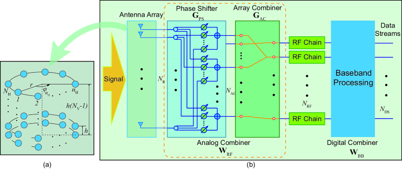
Fig. 2: (a) The geometric model of the UCyA; (b) The block diagram of hybrid beamforming architecture.

III Proposed Two-Step Wideband Hybrid Beamforming Strategy

In this section, new hybrid beamformers are designed to select the meaningful beams needed vertically for angle and delay estimation, and transform the received high-dimensional signals of horizontal UCAs to be low-dimensional by taking Q-DFT and the convergence property of the Bessel function. We prove that the number of low dimensions does not grow with the number of antennas per UCA. The minimal number of required RF chains is the product of the number of vertical beams and the number of low dimensions.

It is worth mentioning that all the beamformers we design here are linear transforms. Therefore, the critical invariance structure for the validity of ESPRIT for the angle and delay estimation, can be recovered losslessly between respective submatrices of the space-time response matrix for the subsequent angle and delay estimation.

III-A Step 1: Vertical Beam Selection

We first propose a new hybrid beamformer, denoted by $\mathbf{W}_{\textrm{s1}}$, in the vertical beamspace. By exploiting the sparsity (or low rank) nature of mmWave multi-antenna channels, the vertical beams can be selected: i) to estimate the number of paths; and ii) to determine the number of vertical beams needed for the joint angle and delay estimation (JADE) (to be developed in Section IV-A).

The output signal after the vertical beamforming is $\mathbf{y}_{\textrm{s1,}m}=\mathbf{W}_{\textrm{s1}}^{H}\mathbf{r}_{m}\in\mathbb{C}^{N_{\textrm{DS},1}\times 1}.$ The hybrid beamformer conducts vertical beamspace transforming and can be constructed as $\mathbf{W}_{\textrm{s1}}=\mathbf{G}_{\textrm{PS},\textrm{s1}}\mathbf{G}_{\textrm{AC},\textrm{s1}}\mathbf{W}_{\textrm{BB},\textrm{s1}},$ where $\mathbf{W}_{\textrm{BB},\textrm{s1}}=\frac{1}{\sqrt{N_{\textrm{V}}}}\mathbf{I}_{N_{\textrm{V}}}\in\mathbb{C}^{N_{\textrm{V}}\times N_{\textrm{V}}}$, $\mathbf{G}_{\textrm{PS},\textrm{s1}}=\mathbf{U}_{\textrm{d}}\otimes\mathbf{I}_{N_{\textrm{H}}}\in\mathbb{C}^{N_{\textrm{R}}\times N_{\textrm{R}}}$, and $\mathbf{G}_{\textrm{AC},\textrm{s1}}=\left[\mathbf{I}_{N_{\textrm{V}}}\otimes\mathbf{1}_{N_{\textrm{H}}}^{T}\right]^{T}\in\mathbb{C}^{N_{\textrm{R}}\times N_{\textrm{V}}}.$ Here, $\mathbf{U}_{\textrm{d}}$ contains $N_{\textrm{V}}$ orthogonal array response vectors corresponding to $N_{\textrm{V}}$ vertically, angularly evenly spaced beams. $\mathbf{U}_{\textrm{d}}=\left[\mathbf{U}_{\textrm{d},1},\mathbf{U}_{\textrm{d},2},\ldots,\mathbf{U}_{\textrm{d},N_{\textrm{V}}}\right]\in\mathbb{C}^{N_{\textrm{V}}\times N_{\textrm{V}}},$ where

$$\mathbf{U}_{\textrm{d},i} =[\exp(-j\frac{2\pi}{N_{\textrm{V}}}(-\frac{N_{\textrm{V}}-1}{2})i),\exp(-j\frac{2\pi}{N_{\textrm{V}}}(-\frac{N_{\textrm{V}}-3}{2})i),$$

$$\ldots,\exp(-j\frac{2\pi}{N_{\textrm{V}}}(\frac{N_{\textrm{V}}-1}{2})i)]^{T},\,i=1,2,\ldots,N_{\textrm{V}}.$$ (5)

Thus at this step, the numbers of both data streams and RF chains are equal to that of beams, i.e., $N_{\textrm{DS},1}=N_{\textrm{RF},1}=N_{\textrm{V}}$. The number of array combiners is equal to that of receive antennas, i.e., $N_{\textrm{AC},1}=N_{\textrm{R}}$. The $i$-th element of $\mathbf{y}_{\textrm{s1,}m}$ can be written as

$$\left[\mathbf{y}_{\textrm{s1},m}\right]_{i,1} =\left[\left(\mathbf{G}_{\textrm{PS},\textrm{s1}}\mathbf{G}_{\textrm{AC},\textrm{s1}}\mathbf{W}_{\textrm{BB},\textrm{s1}}\right)^{H}\mathbf{r}_{m}\right]_{i}$$

$$=\frac{1}{\sqrt{N_{\textrm{V}}}}\mathbf{U}_{\textrm{d},i}^{H}(\mathbf{I}_{N_{\textrm{V}}}\otimes\mathbf{1}_{N_{\textrm{H}}}^{T})\mathbf{r}_{m}.$$ (6)

The total beam power at the $m$-th subcarrier is given by

$$\sigma_{m}^{2}=\mathbf{y}_{\textrm{s1},m}^{H}\mathbf{y}_{\textrm{s1,}m}=\sum_{i=1}^{N_{\textrm{V}}}\sigma_{m,i}^{2},$$ (7)

where $\sigma_{m,i}^{2}=\left|\left[\mathbf{y}_{\textrm{s1},m}\right]_{i,1}\right|^{2}$ is the power of the $i$-th beam which depends on the AOA of the impinging signal inside the beam. Given the sparsity of mmWave multi-antenna channels, the signal power is concentrated in a small number of beams. We select the dominant beams at the $m$-th subcarrier by defining an index selection set $\mathcal{U}_{m}$, as given by

$$\mathcal{U}_{m}\triangleq\left\{\eta(1),\eta(2),\ldots,\eta(N_{\textrm{B},m})\right\},$$ (8)

where $N_{\textrm{B},m}$ is the number of selected beams, and $\eta(u_{m})$ is the index for $\sigma_{m,\eta(u_{m})}^{2}$ with $u_{m}=1,2,\ldots,N_{\textrm{B},m}$. $\eta(u_{m})$ can be obtained as

$$\begin{cases}\eta(1)=\arg\max_{i\in\{1,\ldots,N_{\textrm{V}}\}}\sigma_{m,i}^{2},\\ \eta(2)=\arg\max_{i\in\{1,\ldots,N_{\textrm{V}}\}\setminus\{\eta(1)\}}\sigma_{m,i}^{2},\\ \quad\vdots\\ \eta(N_{\textrm{B},m})=\arg\max_{i\in\{1,\ldots,N_{\textrm{V}}\}\setminus\{\eta(1),\ldots,\eta(N_{\textrm{B},m}-1)\}}\sigma_{m,i}^{2}.\end{cases}$$

The following criterion can be used to decide $N_{\textrm{B},m}$ and select the $N_{\textrm{B},m}$ strongest beams:

$$\sum_{u_{m}=1}^{N_{\textrm{B},m}}\sigma_{m,\eta(u_{m})}^{2}\geq\eta\sigma_{m}^{2},$$ (9)

where $\eta$ is a power threshold which can be empirically specified. $\eta$ can be selected close to 1, e.g., $\eta=0.9$, as paths reflected more than once, and diffuse scattering, account for less than 10% of the total energy, as found in [29]. Moreover, mmWave signals fade rapidly when reflecting off a surface [30], and become barely distinguishable from noises after two reflections [31, 10, 29].

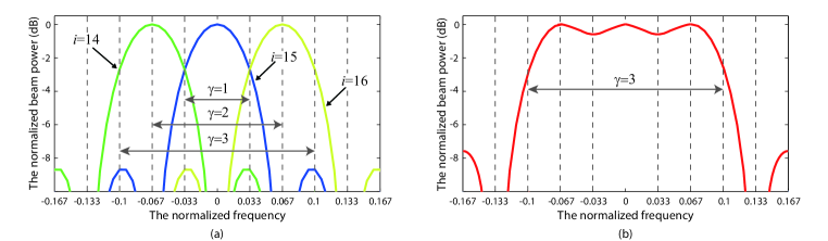
Fig. 3: The normalized beam power as a function of the normalized frequency. (a) The power of the$14$-th, $15$-th, and $16$-th beams; (b) The power of the combined three beams.

There is dispersion in the angular domain across the bandwidth in multi-antenna wireless systems [19]. We first assume that the transmission channel at each subcarrier is narrowband. Because of small dispersion in narrowband systems, the number of orthogonal beams in the vertical beamspace is equal to the number of received paths, i.e., $N_{\textrm{B},m}=N_{\textrm{p}}$ [19]. However, the dispersion can have a non-negligible effect in broadband systems, such as the one considered in this paper, where a point source spreads across spatial angle and time. A strong dispersion would result in severe power loss and pulse distortion, if not addressed properly, and affect the follow-on angle and delay estimation. The dispersion effect can be characterized by the channel dispersion factor, $\gamma$, as specified by [19]

$$\gamma=\frac{1}{N_{\textrm{p}}}\sum_{l=1}^{N_{\textrm{p}}}\gamma_{l}=\frac{1}{N_{\textrm{p}}}\sum_{l=1}^{N_{\textrm{p}}}N_{\textrm{V}}\alpha\left|\chi_{\textrm{c},l}\right|,$$ (10)

where $\alpha=W/f_{\textrm{c}}$ is the fractional bandwidth, $\chi_{\textrm{c},l}=f_{\textrm{c}}h\cos(\theta_{\textrm{R},l})/c$ is the normalized beam angle, $W$ is the signal bandwidth, and $f_{\textrm{c}}$ is the center frequency.

To illustrate the impact of the dispersion, we assume that the system operates at $f_{\textrm{c}}=$30 GHz and the transmitted signal has unit amplitude. For simplicity, it is assumed that only one path with $\beta_{l}=1$ and $\theta_{\textrm{R},l}=60^{\circ}$, and the number of beams is $N_{\textrm{V}}=60$. We have $\chi_{\textrm{c},l}\approx 0.25$, which corresponds to the $i_{0}=15$-th beam. Fig. 3(a) shows the normalized power, $\left|\mathbf{y}_{\textrm{s1},i}(f)\right|^{2}/N_{\textrm{V}}$, of the $14$-th, $15$-th, and $16$-th beams versus the normalized frequency, $f_{\textrm{normal}}=f/f_{\textrm{c}},$ for $f\in[-W/2,W/2]$. We can see that, if the normalized frequency $f_{\textrm{normal}}<0.033,$ i.e., the channel dispersion factor $\gamma<1$, the beams in Fig. 3(a) do not affect one another within the bandwidth, $W$. If $\gamma>1$, power loss and interference may occur. To prevent this from happening, the $\gamma$ adjacent beams centered at $i_{0}$ need to be taken into consideration. In the case of $\gamma=3$, Fig. 3(b) plots the normalized power of the three beams combined, i.e., the $14$-th, $15$-th, and $16$-th beams. It can be seen that, by combining the three beams, the normalized power becomes approximately flat across the operating band.

Because of the dispersion, we have to jointly consider $N_{\textrm{B}}=\gamma N_{\textrm{p}}$ vertically spaced beams to include all possible beams, as the normalized beam angle, $\chi_{\textrm{c},l}$, is unknown. The overall index selection set $\mathcal{U}$ is given by

$$\mathcal{U}=\mathcal{U}_{0}\cup\mathcal{U}_{1}\cup\ldots\cup\mathcal{U}_{M-1},$$ (11)

where the elements of $\mathcal{U}$ are $\eta(u)$ with $u=1,2,\ldots,N_{\textrm{B}}.$ It is possible that the same indices are picked up at different subcarriers because of the dispersion, e.g., $\eta(u_{m})=\eta(u_{m^{\prime}})$ for $m^{\prime}\in\{0,\ldots,M-1\}\setminus\{m\}$. We have $N_{\textrm{B}}=\gamma N_{\textrm{p}}\leq\sum_{m=0}^{M-1}N_{\textrm{B},m}$ to avoid overlooking significant paths in the subsequent joint delay and angle estimation process. Algorithm 1 summarizes the procedure of the beam selection at this step.

Algorithm 1 Beam selection algorithm

• Input: The processed signals, $\mathbf{y}_{\textrm{s1,}m}$,$(m=0,1,\ldots,M-1)$, the beam number, $N_{\textrm{V}}$, and the threshold, $\eta$.

• Output: The overall selection set, $\mathcal{U}$, and the estimated number of significant beams, $N_{\textrm{B}}$.

• Initialization: $\mathcal{U}=\mathcal{U}_{0}=\mathcal{U}_{1}=\ldots=\mathcal{U}_{M-1}=\emptyset$,

• For $m=0$ to $M-1$ do

  • Set $\mathcal{V}=\emptyset.$

  • For $i=1$ to $N_{\textrm{V}}$ do

    • $\sigma_{m,i}^{2}=\left|\mathbf{y}_{\textrm{s1},m,i}\right|^{2}$, and update$\mathcal{V}=\mathcal{V}\cup\{\sigma_{m,i}^{2}\}$.

  • End for

  • $\sigma_{m}^{2}=\sum_{i=1}^{N_{\textrm{V}}}\sigma_{m,i}^{2}.$

  • While $\sum_{\eta(u_{m})\in\mathcal{U}_{m}}\sigma_{m,\eta(u_{m})}^{2}<\eta\sigma_{m}^{2}$ do

    • Find the largest $\sigma_{m,i}^{2}$ from $\mathcal{V}$, and update $\mathcal{U}_{m}=\mathcal{U}_{m}\cup\{i\}$ and $\mathcal{V}=\mathcal{V}\setminus\{\sigma_{m,i}^{2}\}$.

  • End while

  • Update $\mathcal{U}=\mathcal{U}\cup\mathcal{U}_{m}$.

• End for

• $N_{\textrm{B}}=$Card$(\mathcal{U})$.

III-B Step 2: Horizontal Q-DFT Beamforming

We proceed to design a new hybrid beamformer to transform the high-dimensional signals of each UCA to a low dimension requiring much fewer RF chains than array elements. This is achieved by first applying Q-DFT to the signals and then exploiting the convergence property of the Bessel function to remove insignificant dimensions.

We first derive an approximate expression for the array response vector to explain the design rationale of this step. According to the Jacobi-Anger expansion [32], the $n_{\textrm{H}}$-th array response vector on the horizontal plane can be written as

$$[\mathbf{a}_{\textrm{H},m}(\phi_{\mathrm{\textrm{R}},l},\theta_{\mathrm{\textrm{R}},l})]_{n_{\textrm{H}},1}=\frac{1}{\sqrt{N_{\textrm{H}}}}e^{j\varpi_{m,l}\cos(\phi_{\textrm{R},l}-\varphi_{n_{\textrm{H}}})}$$

$$=\frac{1}{\sqrt{N_{\textrm{H}}}}\sum_{q=-\infty}^{\infty}j^{q}J_{q}(\varpi_{m,l})e^{jq(\phi_{\textrm{R},l}-\varphi_{n_{\textrm{H}}})},$$ (12)

where $\varpi_{m,l}=\frac{2\pi}{c}f_{m}r\sin(\theta_{\textrm{R},l})$ and $J_{q}(\varpi_{m,l})$ is the Bessel function of the first kind of order $q$.

We notice that the last multiplier in (12), i.e., $e^{jq(\phi_{\textrm{R},l}-\varphi_{n_{\textrm{H}}})}=e^{jq\phi_{\textrm{R},l}-j2\pi q(n_{\mathrm{H}}-1)/N_{\mathrm{H}}},$ is of strong resemblance to the weight vectors in the DFT. We take the Q-DFT [33] to transform the horizontal array response vectors (12) to offset $\varphi_{n_{\textrm{H}}}$. The $p$-th order Q-DFT of (12) can be expressed as

$$A_{\textrm{PM},p}=\sum_{n_{\textrm{H}}=1}^{N_{\textrm{H}}}\left([\mathbf{a}_{\textrm{H},m}(\phi_{\mathrm{\textrm{R}},l},\theta_{\mathrm{\textrm{R}},l})]_{n_{\textrm{H}},1}\right)e^{-j\frac{2\pi(n_{\mathrm{H}}-1)}{N_{\mathrm{H}}}p}$$

$$=\frac{1}{\sqrt{N_{\textrm{H}}}}\sum_{n_{\textrm{H}}=1}^{N_{\textrm{H}}}\sum_{q=-\infty}^{\infty}j^{q}J_{q}(\varpi_{m,l})e{}^{jq(\phi_{\textrm{R},l}-\varphi_{n_{\textrm{H}}})-jp\varphi_{n_{\textrm{H}}}}$$

$$=\frac{1}{\sqrt{N_{\textrm{H}}}}\sum_{n_{\textrm{H}}=1}^{N_{\textrm{H}}}\left(\sum_{q=-\infty}^{\infty}j^{q}J_{q}(\varpi_{m,l})e^{-j\varphi_{n_{\textrm{H}}}(p+q)}e^{jq\phi_{\textrm{R},l}}\right).$$ (13)

Let $p+q=QN_{\mathrm{H}}$, i.e., $q=QN_{\mathrm{H}}-p$. Then, (13) can be rewritten as

$$A_{\textrm{PM},p} =\frac{1}{\sqrt{N_{\textrm{H}}}}\sum_{Q=-\infty}^{\infty}N_{\textrm{H}}j^{(QN_{\mathrm{H}}-p)}$$

$$\times J_{(QN_{\mathrm{H}}-p)}(\varpi_{m,l})e^{j(QN_{\mathrm{H}}-p)\phi_{\textrm{R},l}}$$

$$\stackrel{{\scriptstyle(\star)}}{{=}}\sqrt{N_{\textrm{H}}}\left[j^{p}J_{p}(\varpi_{m,l})e^{-jp\phi_{\textrm{R},l}}\vphantom{\sum_{Q=-\infty,Q\neq 0}^{\infty}}\right.$$

$$\left.+\sum_{Q=-\infty,Q\neq 0}^{\infty}\varepsilon_{p,Q}(\varpi_{m,l},\phi_{\textrm{R},l})\right],$$ (14)

where

$$\varepsilon_{p,Q}(\varpi_{m,l},\phi_{\textrm{R},l})=j^{(QN_{\mathrm{H}}-p)}J_{(QN_{\mathrm{H}}-p)}(\varpi_{m,l})e^{j(QN_{\mathrm{H}}-p)\phi_{\textrm{R},l}}.$$

$(\star)$ is obtained by the property of the Bessel function $J_{-v}(x)=(-1)^{v}J_{v}(x)$ [32].

Lemma 1. For the Bessel function $J_{v}(x)$, when its order $v$ is larger than its argument $x$, i.e., $\left|v\right|>\left|x\right|$, the amplitude of $J_{v}(x)$ is so small and negligible, i.e., $\left|J_{v}(x)\right|\approx 0.$

Proof. See Appendix I.

From Lemma 1, we can derive the following theorem on the approximation of the horizontal array response vector.

Theorem 1. If $N_{\mathrm{H}}\geq 2P$, the $N_{\mathrm{H}}$-dimensional array response vectors on the horizontal plane can be transformed to a much smaller $(2P+1)$-dimensional space with negligible loss, i.e., $p\in[-P,P]\cap\mathbb{Z}$, where $P=\left\lfloor 2\pi f_{0}r/c\right\rfloor$ is the highest order. The $p$-th order of the $(2P+1)$-dimensional vector, $A_{\textrm{PM},p},$ can be approximated as $A_{\textrm{PM},p}\approx\sqrt{N_{\textrm{H}}}j^{p}J_{p}(\varpi_{m,l})\exp\left(-jp\phi_{\textrm{R},l}\right).$

Proof. See Appendix II.

According to Theorem 1, we see that, by using the Q-DFT, the $N_{\textrm{H}}$-dimensional array response vectors of the horizontal UCA can be transformed to only $(2P+1)$ dimensions, and each element of the vector can be approximately expressed as an exponential function weighted by a Bessel function of the same order, as long as the conditions in Theorem 1, i.e., $N_{\textrm{H}}\geq 2P$, is met.

We note that Q-DFT is a linear transform and hence can preserve the multiple-invariance structure of the array response vectors for the subsequent angle and delay estimation, as will be elaborated on in Section IV-A; see (32) and (39). Thus, combining with the beams selected at Step 1, we can design the values of the phase shifters based on the Q-DFT and the beamspace transform to convert the array response vectors to a low dimension. Only a small number of RF chains are needed for the delay and angle estimation.

At this step, the hybrid beamformer is $\mathbf{W}_{\textrm{s2}}=\mathbf{G}_{\textrm{PS},\textrm{s2}}\mathbf{G}_{\textrm{AC},\textrm{s2}}\mathbf{W}_{\textrm{BB},\textrm{s2}}$. Then we have

$$\mathbf{y}_{\textrm{s2,}m}=\mathbf{W}_{\textrm{s2}}^{H}\mathbf{r}_{m}=(\mathbf{G}_{\textrm{PS},\textrm{s2}}\mathbf{G}_{\textrm{AC},\textrm{s2}}\mathbf{W}_{\textrm{BB},\textrm{s2}})^{H}\mathbf{r}_{m}\in\mathbb{C}^{N_{\textrm{DS},2}\times 1},$$ (15)

where $\mathbf{W}_{\textrm{BB},\textrm{s2}}=\sqrt{N_{\textrm{V}}/N_{\textrm{H}}}\mathbf{I}_{(2P+1)N_{\textrm{B}}}\in\mathbb{C}^{(2P+1)N_{\textrm{B}}\times(2P+1)N_{\textrm{B}}}$, $\mathbf{J}_{\textrm{B}}=[\mathbf{J}_{\textrm{B},1},\mathbf{J}_{\textrm{B},2},\ldots,\mathbf{J}_{\textrm{B},N_{\textrm{B}}}]\in\mathbb{R}^{N_{\textrm{V}}\times N_{\textrm{B}}}$, and $\mathbf{G}_{\textrm{AC},\textrm{s2}}=\mathbf{J}_{\textrm{B}}\otimes\mathbf{I}_{(2P+1)}\in\mathbb{R}^{(2P+1)N_{\textrm{V}}\times(2P+1)N_{\textrm{B}}}$. The elements of $\mathbf{J}_{\textrm{B},u}\in\mathbb{R}^{N_{\textrm{V}}\times 1}$ are given by

$$\left[\mathbf{J}_{\textrm{B},u}\right]_{n_{\textrm{V}},1}=\begin{cases}1,&\textrm{if }n_{\textrm{V}}=\eta(u);\\ 0,&\textrm{otherwise.}\end{cases}$$

We design the phase shifter set of the analog part of the hybrid array, as $\mathbf{G}_{\textrm{PS},\textrm{s2}}=\mathbf{U}_{\textrm{d}}\otimes\mathbf{U}_{\textrm{sH}}\in\mathbb{C}^{N_{\textrm{R}}\times(2P+1)N_{\textrm{V}}},$ where $\mathbf{U}_{\textrm{d}}$ is given in (5) and the element of $\mathbf{U}_{\textrm{sH}}\in\mathbb{C}^{N_{\textrm{H}}\times(2P+1)}$ can be expressed as $\left[\mathbf{U}_{\textrm{sH}}\right]_{n_{\mathrm{H}},p+P+1}=e{}^{j2\pi(n_{\mathrm{H}}-1)p/N_{\mathrm{H}}}$. Hence, the analog combiner of the hybrid array can be constructed as

$$\mathbf{W}_{\textrm{RF},\textrm{s2}} =\mathbf{G}_{\textrm{PS},\textrm{s2}}\mathbf{G}_{\textrm{AC},\textrm{s2}}=(\mathbf{U}_{\textrm{d}}\otimes\mathbf{U}_{\textrm{sH}})(\mathbf{J}_{\textrm{B}}\otimes\mathbf{I}_{(2P+1)})$$

$$\stackrel{{\scriptstyle(\star)}}{{=}}(\mathbf{U}_{\textrm{d}}\mathbf{J}_{\textrm{B}})\otimes(\mathbf{U}_{\textrm{sH1}}\mathbf{I}_{(2P+1)})=\mathbf{U}_{\textrm{sV}}\otimes\mathbf{U}_{\textrm{sH}},$$ (16)

where $(\star)$ follows a property of the Khatri-Rao product, i.e., $(\mathbf{A}\otimes\mathbf{B})(\mathbf{C}\otimes\mathbf{D})=\mathbf{AC}\otimes\mathbf{BD}$. The element of $\mathbf{U}_{\textrm{sV}}\in\mathbb{C}^{N_{\textrm{V}}\times N_{\textrm{B}}}$ can be calculated as $\left[\mathbf{U}_{\textrm{sV}}\right]_{n_{\textrm{V}},u}=\exp(-j\frac{2\pi}{N_{\textrm{V}}}(\frac{N_{\textrm{V}}+1}{2}-n_{\textrm{V}})\eta(u))$. As a result, at this step we have $N_{\textrm{DS},2}=N_{\textrm{RF},2}=(2P+1)N_{\textrm{B}}$ data streams and RF chains, and $N_{\textrm{AC,2}}=(2P+1)N_{\textrm{V}}$ array combiners. The processed received signal in (15) can be written as

$$\mathbf{y}_{\textrm{s2,}m} =\mathbf{W}_{\textrm{s2}}^{H}\mathbf{r}_{m}$$

$$=(\mathbf{G}_{\textrm{s2}}\mathbf{W}_{\textrm{RF},\textrm{s2}}\mathbf{W}_{\textrm{BB},\textrm{s2}})^{H}\mathbf{H}_{m}x_{m}+\mathbf{W}_{\textrm{s2,}m}^{H}\mathbf{n}_{m}$$

$$=\sqrt{\frac{N_{\textrm{V}}}{N_{\textrm{H}}}}(\mathbf{U}_{\textrm{sV}}\otimes\mathbf{U}_{\textrm{sH}})^{H}\sum_{l=1}^{N_{\textrm{p}}}\beta_{l}x_{m}e^{-j2\pi f_{m}\tau_{l}}$$

$$\qquad\times\mathbf{a}_{m}(\phi_{\mathrm{\textrm{R}},l},\theta_{\mathrm{\textrm{R}},l})+\mathbf{W}_{\textrm{s2,}m}^{H}\mathbf{n}_{m}$$

$$\stackrel{{\scriptstyle(\star)}}{{=}}\sqrt{\frac{N_{\textrm{V}}}{N_{\textrm{H}}}}\sum_{l=1}^{N_{\textrm{p}}}\beta_{l}x_{m}e^{-j2\pi f_{m}\tau_{l}}(\mathbf{U}_{\textrm{sV}}^{H}\otimes\mathbf{U}_{\textrm{sH}}^{H})$$

$$\qquad\times(\mathbf{a}_{\textrm{V},m}(\theta_{\mathrm{\textrm{R}},l})\otimes\mathbf{a}_{\textrm{H},m}(\phi_{\mathrm{\textrm{R}},l},\theta_{\mathrm{\textrm{R}},l}))+\mathbf{W}_{\textrm{s2,}m}^{H}\mathbf{n}_{m}$$

$$=\sum_{l=1}^{N_{\textrm{p}}}\beta_{l}x_{m}e^{-j2\pi f_{m}\tau_{l}}(\sqrt{N_{\textrm{V}}}\mathbf{U}_{\textrm{sV}}^{H}\mathbf{a}_{\textrm{V},m}(\theta_{\mathrm{\textrm{R}},l}))$$

$$\qquad\otimes(\frac{1}{\sqrt{N_{\textrm{H}}}}\mathbf{U}_{\textrm{sH}}^{H}\mathbf{a}_{\textrm{H},m}(\phi_{\mathrm{\textrm{R}},l},\theta_{\mathrm{\textrm{R}},l}))+\mathbf{W}_{\textrm{s2,}m}^{H}\mathbf{n}_{m}$$

$$=\sum_{l=1}^{N_{\textrm{p}}}\beta_{l}x_{m}e^{-j2\pi f_{m}\tau_{l}}(\tilde{\mathbf{a}}_{\textrm{V},m}(\theta_{\mathrm{\textrm{R}},l})$$

$$\qquad\otimes\tilde{\mathbf{a}}_{\textrm{H},m}(\phi_{\mathrm{\textrm{R}},l},\theta_{\mathrm{\textrm{R}},l}))+\mathbf{W}_{\textrm{s2,}m}^{H}\mathbf{n}_{m},$$ (17)

where $(\star)$ stems from another property of the Khatri-Rao product, i.e., $(\mathbf{A}\otimes\mathbf{B})^{H}=\mathbf{A}^{H}\otimes\mathbf{B}^{H}$. According to Theorem 1, the elements of the resulting vertical and horizontal array response vectors $\tilde{\mathbf{a}}_{\textrm{V},m}(\theta_{\mathrm{\textrm{R}},l})$ and $\tilde{\mathbf{a}}_{\textrm{H},m}(\phi_{\mathrm{\textrm{R}},l},\theta_{\mathrm{\textrm{R}},l})$ are given by

$$[\tilde{\mathbf{a}}_{\textrm{V},m}(\theta_{\mathrm{\textrm{R}},l})]_{u,1}=\sqrt{N_{\textrm{V}}}\mathbf{U}_{\textrm{sV}}^{H}\mathbf{a}_{\textrm{V},m}(\theta_{\mathrm{\textrm{R}},l})$$

$$\qquad=\sum_{n_{\textrm{V}}=1}^{N_{\textrm{V}}}\exp\left(-j\frac{2\pi}{c}f_{m}h(n_{\textrm{V}}-\frac{N_{\textrm{V}}+1}{2})\cos(\theta_{\textrm{R},l})\right)$$

$$\qquad\qquad\times\exp\left(j\frac{2\pi}{N_{\textrm{V}}}(\frac{N_{\textrm{V}}+1}{2}-n_{\textrm{V}})\eta(u)\right)$$

$$\qquad=\frac{\sin\left(N_{\textrm{V}}(2\pi f_{m}h\cos(\theta_{\textrm{R},l})/c-2\pi\eta(u)/N_{\textrm{V}})/2\right)}{\sin\left((2\pi f_{m}h\cos(\theta_{\textrm{R},l})/c-2\pi\eta(u)/N_{\textrm{V}})/2\right)}$$ (18)

and

$$[\tilde{\mathbf{a}}_{\textrm{H},m}(\phi_{\mathrm{\textrm{R}},l},\theta_{\mathrm{\textrm{R}},l})]_{p+P+1,1}=\frac{1}{\sqrt{N_{\textrm{H}}}}\mathbf{U}_{\textrm{sH}}^{H}\mathbf{a}_{\textrm{H},m}(\phi_{\mathrm{\textrm{R}},l},\theta_{\mathrm{\textrm{R}},l})$$

$$=\frac{1}{\sqrt{N_{\textrm{H}}}}A_{\textrm{PM},p}\approx j^{p}J_{p}(\varpi_{m,l})e^{-jp\phi_{\textrm{R},l}}.$$ (19)

Steps 1 and 2 are indispensable, reducing the number of required RF chains substantially from $N_{\textrm{R}}$ to $(2P+1)N_{\textrm{B}}$.

III-C Multidimensional Spatial Interpolation (MDSI)

When the fractional bandwidth or the scale of the antenna array is large, the aforementioned beam squint effect arises [19]. This is because the array response vectors (18) and (19) depend on the frequency of the specific subcarrier $f_{m}$. The beam squint effect would compromise the capability of jointly utilizing the received signals at all frequency bands to estimate the path parameters. As a result, the high temporal resolution of wideband mmWave systems could not be effectively exploited.

One could keep the array response matrices consistent across all frequencies, by transforming the array response vectors (18) and (19) associated with the frequency $f_{m}$, $\forall m=0,1,\ldots,M-1$, into the corresponding array response vectors at the reference frequency $f_{0}$ [23]. For continuous signals, this could be ideally achieved by the Shannon-Whittaker interpolation [34], which sets different vertical distances and radii at different frequencies, i.e., $h_{\textrm{vi},m}=f_{0}h/f_{m}$ and $r_{\textrm{vi},m}=f_{0}r/f_{m}$. Then, from (18) and (19), the virtual vertical and horizontal response vectors, $\mathbf{\dot{a}}_{\textrm{V},m}(\theta_{\mathrm{\textrm{R}},l})$ and $\mathbf{\dot{a}}_{\textrm{H},m}(\theta_{\mathrm{\textrm{R}},l})$, can be constructed as

$$[\mathbf{\dot{a}}_{\textrm{V},m}(\theta_{\mathrm{\textrm{R}},l})]_{u,1}$$

$$=\frac{\sin\left(N_{\textrm{V}}(2\pi f_{m}h_{\textrm{vi},m}\cos(\theta_{\textrm{R},l})/c-2\pi\eta(u)/N_{\textrm{V}})/2\right)}{\sin\left((2\pi f_{m}h_{\textrm{vi},m}\cos(\theta_{\textrm{R},l})/c-2\pi\eta(u)/N_{\textrm{V}})/2\right)}$$

$$=\frac{\sin\left(N_{\textrm{V}}(2\pi f_{0}h\cos(\theta_{\textrm{R},l})/c-2\pi\eta(u)/N_{\textrm{V}})/2\right)}{\sin\left((2\pi f_{0}h\cos(\theta_{\textrm{R},l})/c-2\pi\eta(u)/N_{\textrm{V}})/2\right)}$$

$$=[\tilde{\mathbf{a}}_{\textrm{V},0}(\theta_{\mathrm{\textrm{R}},l})]_{u,1}$$ (20)

and

$$[\mathbf{\dot{a}}_{\textrm{H},m}(\phi_{\mathrm{\textrm{R}},l},\theta_{\mathrm{\textrm{R}},l})]_{p+P+1,1}$$

$$=j^{p}J_{p}(\frac{2\pi}{c}f_{m}r_{\textrm{vi},m}\sin(\theta_{\textrm{R},l}))e^{-jp\phi_{\textrm{R},l}}$$

$$=j^{p}J_{p}(\frac{2\pi}{c}f_{0}r\sin(\theta_{\textrm{R},l}))e^{-jp\phi_{\textrm{R},l}}$$

$$=[\tilde{\mathbf{a}}_{\textrm{H},0}(\phi_{\mathrm{\textrm{R}},l},\theta_{\mathrm{\textrm{R}},l})]_{p+P+1,1}.$$ (21)

The signal reconstructed by using (20) and (21) can be expressed as

$$\mathbf{\dot{y}}_{\textrm{s2,}m}=\sum_{l=1}^{N_{\textrm{p}}}\beta_{l}x_{m}e^{-j2\pi f_{m}\tau_{l}}(\mathbf{\dot{a}}_{\textrm{V},m}(\theta_{\mathrm{\textrm{R}},l})$$

$$\qquad\otimes\mathbf{\dot{a}}_{\textrm{H},m}(\phi_{\mathrm{\textrm{R}},l},\theta_{\mathrm{\textrm{R}},l}))+\mathbf{W}_{\textrm{s2,}m}^{H}\mathbf{n}_{m}$$

$$=\sum_{l=1}^{N_{\textrm{p}}}\beta_{l}x_{m}e^{-j2\pi f_{m}\tau_{l}}(\tilde{\mathbf{a}}_{\textrm{V},0}(\theta_{\mathrm{\textrm{R}},l})\otimes\tilde{\mathbf{a}}_{\textrm{H},0}(\phi_{\mathrm{\textrm{R}},l},\theta_{\mathrm{\textrm{R}},l}))$$

$$\qquad+\mathbf{W}_{\textrm{s2,}m}^{H}\mathbf{n}_{m}$$

$$=\sum_{l=1}^{N_{\textrm{p}}}\beta_{l}x_{m}e^{-j2\pi f_{m}\tau_{l}}\tilde{\mathbf{a}}_{0}(\phi_{\mathrm{\textrm{R}},l},\theta_{\mathrm{\textrm{R}},l})+\mathbf{W}_{\textrm{s2,}m}^{H}\mathbf{n}_{m}.$$ (22)

In practice, the Shannon-Whittaker interpolation could hardly achieve perfect signal reconstruction for time-limited signals, and it also has a high computational complexity [34].

In this paper, we extend linear interpolation [35] (which is a low-complexity and effective method for data point construction) to the multidimensional spatial interpolation. The multidimensional array response matrices consistent across all frequencies can be constructed by using the received time-limited signals. By applying the linear interpolation in both the vertical and horizontal spatial domains, we can reconstruct the signal in (17) and obtain an approximation of (22). The reconstructed signal is calculated as

$$\left[\mathbf{\tilde{\mathbf{y}}}_{\textrm{s2,}m}\right]_{n_{\textrm{DS},2},1} =\left[\mathbf{y}_{\textrm{s2,}m}\right]_{n_{\textrm{DS},2},1}+\frac{r_{\textrm{vi},m}}{r}\Delta_{\mathbf{y}_{\textrm{s2,H,}m}}+\frac{h_{\textrm{vi},m}}{h}\Delta_{\mathbf{y}_{\textrm{s2,V,}m}},$$ (23)

where $n_{\textrm{DS},2}=(2P+1)(u-1)+p$. If $n_{\textrm{DS},2}\leq(2P+1)(N_{\textrm{B}}-1)$, $\Delta_{\mathbf{y}_{\textrm{s2,H,}m}}$ and $\Delta_{\mathbf{y}_{\textrm{s2,V,}m}}$ are constructed as $\Delta_{\mathbf{y}_{\textrm{s2,H,}m}}=\left[\mathbf{y}_{\textrm{s2,}m}\right]_{(n_{\textrm{DS},2}+1),1}-\left[\mathbf{y}_{\textrm{s2,}m}\right]_{n_{\textrm{S}},1}$ and $\Delta_{\mathbf{y}_{\textrm{s2,V,}m}}=\left[\mathbf{y}_{\textrm{s2,}m}\right]_{(n_{\textrm{DS},2}+2P+1),1}-\left[\mathbf{y}_{\textrm{s2,}m}\right]_{n_{\textrm{DS},2},1}$, respectively. Otherwise, $\Delta_{\mathbf{y}_{\textrm{s2,H,}m}}=\left[\mathbf{y}_{\textrm{s2,}m}\right]_{n_{\textrm{DS},2},1}-\left[\mathbf{y}_{\textrm{s2,}m}\right]_{(n_{\textrm{DS},2}-1),1}$ and $\Delta_{\mathbf{y}_{\textrm{s2,V,}m}}=\left[\mathbf{y}_{\textrm{s2,}m}\right]_{n_{\textrm{DS},2},1}-\left[\mathbf{y}_{\textrm{s2,}m}\right]_{(n_{\textrm{DS},2}-2P-1),1}.$

IV Proposed Wideband Channel Parameter Estimation

In this section, we estimate the path parameters and the 3D position of the MS based on the processed signals in Sections III and III-C. Since the beamformers developed in Section III are linear transforms, the multiple-invariance structure required for ESPRIT can be recovered losslessly between respective submatrices of the space-time response matrix. By exploiting the recurrence relations in the multiple-invariance structure, the delay and elevation angle of each path can be estimated using ESPRIT. For the azimuth angles, the expression for the horizontal array response vectors (19) does not exhibit any recurrence. Hence the azimuth angles are estimated by using MUSIC after obtaining the corresponding elevation angles. The hardware and software complexities of the proposed joint delay and angle estimation approach are analyzed in the end.

IV-A Wideband JADE Algorithm

Collecting the received signals at all frequencies, we have $\mathbf{\tilde{\mathbf{y}}}=\left[\mathbf{\tilde{\mathbf{y}}}_{\textrm{s2,}1},\mathbf{\tilde{\mathbf{y}}}_{\textrm{s2,}2},\ldots,\mathbf{\tilde{\mathbf{y}}}_{\textrm{s2,}M}\right].$ Assume that the same signals are transmitted at all subcarriers. We can vectorize $\mathbf{\mathbf{\tilde{\mathbf{y}}}}$ as

$$\mathbf{\mathbf{\tilde{\mathbf{y}}}_{\textrm{vec}}}=\textrm{vec}(\mathbf{\mathbf{\tilde{\mathbf{y}}}})=\left[\mathbf{\Gamma}\diamond\tilde{\mathbf{A}}\right]\mathbf{d}+\textrm{vec}(\mathbf{\mathbf{\tilde{\mathbf{n}}}})=\mathbf{U}\mathbf{d}+\tilde{\mathbf{n}}_{\textrm{v}},$$ (24)

where $\tilde{\mathbf{A}}=\left[\tilde{\mathbf{a}}_{0}(\phi_{\mathrm{\textrm{R}},1},\theta_{\mathrm{\textrm{R}},1}),\ldots,\tilde{\mathbf{a}}_{0}(\phi_{\mathrm{\textrm{R}},N_{\textrm{p}}},\theta_{\mathrm{\textrm{R}},N_{\textrm{p}}})\right],$ $\mathbf{\mathbf{\tilde{\mathbf{n}}}}=\mathbf{W}_{\textrm{s2}}^{H}\left[\mathbf{n}_{1},\ldots,\mathbf{n}_{M}\right],$ $\left[\mathbf{\Gamma}\right]_{m,l}=e^{-j2\pi f_{m}\tau_{l}}$, and $\mathbf{d}=x\left[\beta_{1},\beta_{2},\ldots,\beta_{N_{\textrm{p}}}\right]^{T}$. Here, $\mathbf{U}\in\mathbb{C}^{N_{\textrm{DS},2}M\times N_{\textrm{p}}}$, also known as the space-time response matrix in [36], collects the set of AOAs and path delays. The covariance matrix of $\mathbf{\tilde{\mathbf{y}}}_{\textrm{vec}}$ can be calculated as

$$\mathbf{R}_{\mathbf{\tilde{\mathbf{y}}}_{\textrm{vec}}}=\mathbb{E}\left\{\mathbf{\tilde{\mathbf{y}}}_{\textrm{vec}}\mathbf{\tilde{\mathbf{y}}}_{\textrm{vec}}^{H}\right\}=\mathbb{\mathbf{U}}\mathbf{\Lambda}_{\mathbf{d}}\mathbf{U}^{H}+\mathbf{\sigma}_{\textrm{n}}^{2}\mathbf{I}_{(N_{\textrm{DS},2}M)},$$ (25)

where $\mathbf{\Lambda}_{\mathbf{d}}=\mathbb{E}\left\{\mathbf{dd}^{H}\right\}$ is a diagonal matrix. The eigenvalue-decomposition (EVD) of $\mathbf{R}_{\mathbf{\tilde{\mathbf{y}}}_{\textrm{vec}}}$ can be obtained by

$$\mathbf{R}_{\mathbf{\tilde{\mathbf{y}}}_{\textrm{vec}}} =\left[\mathbf{\mathbf{E}_{\textrm{s}}},\mathbf{E}_{\textrm{n}}\right]\left[\begin{array}[]{cc}\mathbf{\Sigma}_{\mathbf{\textrm{s}}}&\mathbf{0}_{N_{\textrm{p}}\times(N_{\textrm{DS},2}M-N_{\textrm{p}})}\\ \mathbf{0}_{(N_{\textrm{DS},2}M-N_{\textrm{p}})\times N_{\textrm{p}}}&\mathbf{\sigma}_{\textrm{n}}^{2}\mathbf{I}_{N_{\textrm{DS},2}M-N_{\textrm{p}}}\end{array}\right]$$ (28)

$$\qquad\times\left[\mathbf{\mathbf{\mathbf{E}_{\textrm{s}}}},\mathbf{E}_{\textrm{n}}\right]^{H}=\mathbf{\mathbf{E}_{\textrm{s}}}\mathbf{\Sigma}_{\mathbf{\textrm{s}}}\mathbf{E}_{\textrm{s}}^{H}+\mathbf{\sigma}_{\textrm{n}}^{2}\mathbf{E}_{\textrm{n}}\mathbf{E}_{\textrm{n}}^{H},$$ (29)

where $\mathbf{E}_{\textrm{s}}\in\mathbf{\mathbb{C}}^{N_{\textrm{DS},2}M\times N_{\textrm{p}}}$ and $\mathbf{\mathbf{E}_{\textrm{n}}\in\mathbb{C}}^{N_{\textrm{DS},2}M\times(N_{\textrm{DS},2}M-N_{\textrm{p}})}$ correspond to the signal subspace and noise subspace, respectively. $\mathbf{\Sigma}_{\mathbf{\textrm{s}}}\in\mathbf{\mathbb{R}}^{N_{\textrm{p}}\times N_{\textrm{p}}}$ is a diagonal matrix whose elements are the $N_{\textrm{p}}$ largest eigenvalues of $\mathbf{R}_{\bar{\mathbf{h}}}$. Based on $\mathbf{E}_{\textrm{n}}\mathbf{E}_{\textrm{n}}^{H}+\mathbf{\mathbf{E}_{\textrm{s}}}\mathbf{E}_{\textrm{s}}^{H}=\mathbf{I}_{N_{\textrm{DS},2}M}$, (29) can be rewritten as

$$\mathbf{R}_{\mathbf{\mathbf{\mathbf{\tilde{\mathbf{y}}}_{\textrm{vec}}}}}=\mathbf{\mathbf{E}_{\textrm{s}}}(\mathbf{\mathbf{\Sigma}_{\mathbf{\textrm{s}}}-\mathbf{\mathbf{\sigma}_{\textrm{n}}^{2}\mathbf{I}}}_{N_{\textrm{p}}})\mathbf{E}_{\textrm{s}}^{H}+\mathbf{\mathbf{\sigma}_{\textrm{n}}^{2}}\mathbf{I}_{N_{\textrm{DS},2}M}.$$ (30)

By setting (25) and (30) equal, we obtain

$$\mathbf{E}_{\textrm{s}}=\mathbf{UT},$$ (31)

where $\mathbf{T}\in\mathbb{C}^{N_{\textrm{p}}\times N_{\textrm{p}}}$ is a full rank matrix.

As discussed below, $\mathbf{U}$ in (31) has a multiple-invariance structure with a linear recurrence relationship. The relationship allows the use of the ESPRIT method to estimate the delay and elevation angle of each path.

IV-A1 Delay Estimation

Define the delay-selection matrix as $\mathbf{J}_{\textrm{D}}=\textrm{diag}\left(\mathbf{J}_{\textrm{D},1},\ldots,\mathbf{J}_{\textrm{D},M}\right)\in\mathbb{R}^{M\times N_{\textrm{DS},2}M},$ where $\mathbf{J}_{\textrm{D},m}=\mathbf{1}_{N_{\textrm{DS},2}}^{T}$. We can obtain the delay-related submatrix $\mathbf{U}_{\textrm{D}}=\mathbf{J}_{\textrm{D}}\mathbf{U}\in\mathbb{C}^{M\times N_{\textrm{p}}}$. By defining $\tilde{\mathbf{J}}_{\textrm{D},m}=[\mathbf{0}_{1\times(m-1)},1,$ $\mathbf{0}_{1\times(M-m)}]\in\mathbb{R}^{1\times M}$, the delay-related submatrix associated with the frequency $f_{m}$ can be calculated as $\mathbf{U}_{\textrm{D},m}=\tilde{\mathbf{J}}_{\textrm{D},m}\mathbf{U}_{\textrm{D}}\in\mathbb{C}^{1\times N_{\textrm{p}}}$. Thus, we obtain a linear recurrence relation between the delay-related submatrices of each frequency as

$$\mathbf{U}_{\textrm{D},\tilde{m}+1}=\mathbf{U}_{\textrm{D},\tilde{m}}\mathbf{\mathbf{\Theta}_{\textrm{D}}},$$ (32)

where $\mathbf{\mathbf{\Theta}_{\textrm{D}}}=\textrm{diag}\left(e^{-j2\pi\Delta_{\textrm{F}}\tau_{1}},\ldots,e^{-j2\pi\Delta_{\textrm{F}}\tau_{N_{\textrm{p}}}}\right)\in\mathbb{C}^{N_{\textrm{p}}\times N_{\textrm{p}}}$ and $\tilde{m}=1,2,\ldots,M-1.$

According to (31), the delay-related submatrix of the signal subspace matrix at the frequency $f_{m}$ can be given by

$$\mathbf{E}_{\textrm{D},m}=\tilde{\mathbf{J}}_{\textrm{D},m}\mathbf{J}_{\textrm{D}}\mathbf{\mathbf{E}_{\textrm{s}}}=\mathbf{U}_{\textrm{D},m}\mathbf{T}.$$ (33)

Substituting (32) into (33), we obtain

$$\mathbf{E}_{\textrm{D},\tilde{m}+1}=\mathbf{E}_{\textrm{D},\tilde{m}}\mathbf{T}^{-1}\mathbf{\mathbf{\Theta}_{\textrm{D}}T}=\mathbf{E}_{\textrm{D},\tilde{m}}\mathbf{\Psi_{\textrm{D}}}.$$ (34)

By using the total least-squares (TLS) criterion [15], we estimate $\Psi_{\textrm{D}}=\mathbf{T}^{-1}\mathbf{\mathbf{\Theta}_{\textrm{D}}T}=\mathbf{E}_{\textrm{D},\tilde{m}}^{\dagger}\mathbf{E}_{\textrm{D},\tilde{m}+1}$ as $\hat{\mathbf{\Psi}}_{\textrm{D},\tilde{m}}$, each of which has a total of $N_{\textrm{p}}$ sorted eigenvalues, i.e., $\lambda_{\textrm{D},\tilde{m},N_{\textrm{p}}}$. Due to the fact that the eigenvalues of an upper triangular matrix are also diagonal elements of the matrix, we can obtain $(M-1)$ different estimates for each $\mathbf{\mathbf{\Theta}_{\textrm{D}}}$. As a result, the delay of the $n_{\textrm{p}}$-th path, $\tau_{n_{\textrm{p}}}$, can be estimated as

$$\hat{\tau}_{l}=\frac{1}{M-1}\sum_{\tilde{m}}^{M-1}\left[j\ln(\lambda_{\textrm{D},\tilde{m},l})/2\pi\Delta_{\textrm{F}}\right].$$ (35)

IV-A2 Angle Estimation

We first use the processed vertical array response vector (20) to estimate the elevation angle. According to (18), the $(u+1)$-th element of $\tilde{\mathbf{a}}_{\textrm{V},0}(\theta_{\mathrm{\textrm{R}},l})$ can be given by

$$[\tilde{\mathbf{a}}_{\textrm{V},0}(\theta_{\mathrm{\textrm{R}},l})]_{u+1,1}$$

$$=\frac{\sin\left(N_{\textrm{V}}(2\pi f_{0}h\cos(\theta_{\textrm{R},l})/c-2\pi\eta(u+1)/N_{\textrm{V}})/2\right)}{\sin\left((2\pi f_{0}h\cos(\theta_{\textrm{R},l})/c-2\pi\eta(u+1)/N_{\textrm{V}})/2\right)}.$$ (36)

Comparing $[\tilde{\mathbf{a}}_{\textrm{V},0}(\theta_{\mathrm{\textrm{R}},l})]_{u+1,1}$ with the $u$-th element in (20), we see that two successive components of the processed vertical array response vector, $[\tilde{\mathbf{a}}_{\textrm{V},0}(\theta_{\mathrm{\textrm{R}},l})]_{u,1}$ and $[\tilde{\mathbf{a}}_{\textrm{V},0}(\theta_{\mathrm{\textrm{R}},l})]_{u+1,1}$, are related as follows.

$$(-1)^{\eta(u)}\sin\left((g(\theta_{\textrm{R},l})-2\pi\eta(u)/N_{\textrm{V}})/2\right)[\tilde{\mathbf{a}}_{\textrm{V},0}(\theta_{\mathrm{\textrm{R}},l})]_{u,1}$$

$$=(-1)^{\eta(u+1)}\sin\left((g(\theta_{\textrm{R},l})-2\pi\eta(u+1)/N_{\textrm{V}})/2\right)$$

$$\qquad\times[\tilde{\mathbf{a}}_{\textrm{V},0}(\theta_{\mathrm{\textrm{R}},l})]_{u+1,1},$$ (37)

where $g(\theta_{\textrm{R},l})=\frac{2\pi}{c}f_{0}h\cos(\theta_{\textrm{R},l})$. By trigonometric manipulations, we rewrite (37) as

$$(-1)^{\eta(u)}\sin\left(\eta(u)\frac{\pi}{N_{\textrm{V}}}\right)[\tilde{\mathbf{a}}_{\textrm{V},0}(\theta_{\mathrm{\textrm{R}},l})]_{u,1}$$

$$\qquad+(-1)^{\eta(u+1)+1}\sin\left(\eta(u+1)\frac{\pi}{N_{\textrm{V}}}\right)[\tilde{\mathbf{a}}_{\textrm{V},0}(\theta_{\mathrm{\textrm{R}},l})]_{u+1,1}$$

$$=\tan\left(\frac{g(\theta_{\textrm{R},l})}{2}\right)\left[(-1)^{\eta(u)}\cos\left(\eta(u)\frac{\pi}{N_{\textrm{V}}}\right)[\tilde{\mathbf{a}}_{\textrm{V},0}(\theta_{\mathrm{\textrm{R}},l})]_{u,1}\right.$$

$$\qquad\left.+(-1)^{\eta(u+1)+1}\cos\left(\eta(u+1)\frac{\pi}{N_{\textrm{V}}}\right)[\tilde{\mathbf{a}}_{\textrm{V},0}(\theta_{\mathrm{\textrm{R}},l})]_{u+1,1}\right].$$ (38)

Stacking all $(N_{\textrm{B}}-1)$ equations together yields

$$\tan\left(\frac{g(\theta_{\textrm{R},l})}{2}\right)\mathbf{F}_{0}\tilde{\mathbf{a}}_{\textrm{V},0}(\theta_{\mathrm{\textrm{R}},l})=\mathbf{F}_{1}\tilde{\mathbf{a}}_{\textrm{V},0}(\theta_{\mathrm{\textrm{R}},l}),$$ (39)

where

$$\left[\mathbf{F}_{0}\right]_{\tilde{u},u}=$$

$$\begin{cases}(-1)^{\eta(\tilde{u})}\cos(2\pi\eta(\tilde{u})/N_{\textrm{V}}),&\textrm{if }u=\eta(\tilde{u});\\ (-1)^{\eta(\tilde{u}+1)+1}\cos(2\pi\eta(\tilde{u}+1)/N_{\textrm{V}}),&\textrm{if }u=\eta(\tilde{u}+1);\\ 0,&\textrm{otherwise.}\end{cases}$$

$$\left[\mathbf{F}_{1}\right]_{\tilde{u},u}=$$

$$\begin{cases}(-1)^{\eta(\tilde{u})}\sin(2\pi\eta(\tilde{u})/N_{\textrm{V}}),&\textrm{if }u=\eta(\tilde{u});\\ (-1)^{\eta(\tilde{u}+1)+1}\sin(2\pi\eta(\tilde{u}+1)/N_{\textrm{V}}),&\textrm{if }u=\eta(\tilde{u}+1);\\ 0,&\textrm{otherwise.}\end{cases}$$

with $\tilde{u}=1,2,\ldots,N_{\textrm{B}}-1$.

The processes of selecting the angle-related submatrices are similar to that of selecting the delay-related submatrices. Define the angle selection matrix as $\mathbf{J}_{\textrm{A}}=\mathbf{1}_{M}^{T}\otimes\mathbf{I}_{N_{\textrm{DS},2}}\in\mathbb{R}^{N_{\textrm{DS},2}\times N_{\textrm{DS},2}M}$. Then the angle-related submatrix can be formulated as $\mathbf{U}_{\textrm{A}}=\mathbf{J}_{\textrm{A}}\mathbf{U}\in\mathbb{C}^{N_{\textrm{DS},2}\times N_{\textrm{p}}}$. Based on the recurrence relation in (39), we can construct

$$\mathbf{F}_{0}\mathbf{U}_{\textrm{V}}\mathbf{\mathbf{\Theta}_{\textrm{V}}}=\mathbf{F}_{1}\mathbf{U}_{\textrm{V}},$$ (40)

where $\mathbf{\mathbf{\Theta}_{\textrm{V}}}=\textrm{diag}\left(\tan(g(\theta_{\textrm{R},1})/2),\ldots,\tan(g(\theta_{\textrm{R},N_{\textrm{p}}})/2)\right)$ and $\mathbf{U}_{\textrm{V}}=\mathbf{J}_{\textrm{V}}\mathbf{U}_{\textrm{A}}\in\mathbb{C}^{N_{\textrm{B}}\times N_{\textrm{p}}}$ is a submatrix of $\mathbf{U}_{\textrm{A}}$, where $\mathbf{J}_{\textrm{V}}=\mathbf{I}_{(2P+1)}\otimes\mathbf{1}_{N_{\textrm{B}}}^{T}\in\mathbb{R}^{N_{\textrm{B}}\times N_{\textrm{DS},2}}$. Thus, the vertical array response-related submatrix can be calculated as

$$\mathbf{E}_{\textrm{V}}=\mathbf{J}_{\textrm{V}}\mathbf{J}_{\textrm{A}}\mathbf{\mathbf{E}_{\textrm{s}}}=\mathbf{J}_{\textrm{V}}\mathbf{J}_{\textrm{A}}\mathbf{UT}=\mathbf{U}_{\textrm{V}}\mathbf{T}.$$ (41)

Substituting (41) into (40), we can obtain

$$\mathbf{F}_{0}\mathbf{E}_{\textrm{V}}\mathbf{T}^{-1}\mathbf{\mathbf{\Theta}_{\textrm{V}}T}=\mathbf{F}_{0}\mathbf{E}_{\textrm{V}}\mathbf{\Psi_{\textrm{V}}}=\mathbf{F}_{1}\mathbf{E}_{\textrm{V}}.$$ (42)

With reference to the delay estimation in Section IV-A1, the elevation angle of the $l$-th path, $\hat{\theta}_{l}$, can be estimated as

$$\hat{\theta}_{\mathrm{\textrm{R}},l}=\arccos\left(\arctan(\lambda_{\textrm{V},l})/\pi f_{0}h\right),$$ (43)

where $\lambda_{\textrm{V},l}$ is the $l$-th eigenvalue of $\hat{\mathbf{\Psi}}_{\textrm{V}}$, and $\hat{\mathbf{\Psi}}_{\textrm{V}}$ is the estimated matrix of $\mathbf{\Psi_{\textrm{V}}}=\mathbf{T}^{-1}\mathbf{\mathbf{\Theta}_{\textrm{V}}T}$.

According to (19), the expression for each horizontal response vector, which does not have the invariance structure, is an exponential function weighted by the Bessel function. There is no recursive relationship for the azimuth angle estimation. After obtaining the elevation angles, we use MUSIC to estimate their corresponding azimuth angles.

Define $\mathbf{J}_{\textrm{H}}=\mathbf{J}_{\textrm{HA}}\mathbf{J}_{\textrm{A}}\in\mathbb{R}^{(2P+1)\times N_{\textrm{DS},2}M}$, where $\mathbf{J}_{\textrm{HA},u}=\left[\mathbf{I}_{(2P+1)},\mathbf{0}_{(2P+1)\times(2P+1)(N_{\textrm{B}}-1)}\right]\in\mathbb{R}^{(2P+1)\times N_{\textrm{DS},2}}.$ We can obtain the corresponding horizontal signal $\mathbf{\mathbf{\tilde{\mathbf{y}}}_{\textrm{vec,H}}}=\mathbf{J}_{\textrm{H}}\mathbf{\mathbf{\tilde{\mathbf{y}}}_{\textrm{vec}}}\in\mathbb{C}^{(2P+1)\times 1}$. As done in (29), the covariance matrix of $\mathbf{\mathbf{\mathbf{\tilde{\mathbf{y}}}_{\textrm{vec,H}}}}$ can be calculated as $\mathbf{R}_{\mathbf{\mathbf{\tilde{\mathbf{y}}}_{\textrm{vec,H}}}}=\mathbf{\mathbf{E}_{\textrm{s,H}}}\mathbf{\Sigma}_{\mathbf{\textrm{s,H}}}\mathbf{E}_{\textrm{s,H}}^{H}+\mathbf{\sigma}_{\textrm{n}}^{2}\mathbf{E}_{\textrm{n,H}}\mathbf{E}_{\textrm{n,H}}^{H},$ where $\mathbf{E}_{\textrm{s,H}}$ and $\mathbf{E}_{\textrm{n,H}}$ are the signal and noise subspaces of $\mathbf{\mathbf{\tilde{\mathbf{y}}}_{\textrm{vec,H}}}$, respectively.

By substituting the estimate of the $l$-th path, $\hat{\theta}_{\mathrm{\textrm{R}},l}$, in the MUSIC estimator, the azimuth angle of the path can be estimated by

$$\hat{\phi}_{\mathrm{\textrm{R}},l}=\arg\max_{\varPhi}\left\|\mathbf{E}_{\textrm{n,H}}^{H}\tilde{\mathbf{a}}_{\textrm{H},0}(\varPhi,\hat{\theta}_{\mathrm{\textrm{R}},l})\right\|_{\textrm{F}}^{-2},$$ (44)

where $\varPhi$ is the azimuth of the AOA, and can be estimated by 1D search.

IV-B Multipath Parameter Matching

As described above, the estimated channel parameters of each path can be matched automatically in the absence of noises. This is because they have the common factor $\mathbf{T}$, as shown in (31). In the presence of non-negligible noises, there can be a mismatch between the estimated parameters. We take the delay and the elevation AOA for an example. According to (34) and (42), we have $\mathbf{\Psi}_{\textrm{D}}=\mathbf{T}_{\textrm{D}}^{-1}\mathbf{\mathbf{\Theta}_{\textrm{D}}}\mathbf{T}_{\textrm{D}}$ and $\mathbf{\Psi_{\textrm{V}}}=\mathbf{T}_{\textrm{V}}^{-1}\mathbf{\mathbf{\Theta}_{\textrm{V}}}\mathbf{T}_{\textrm{V}}$, but $\mathbf{T}_{\textrm{V}}\neq\mathbf{T}_{\textrm{D}}\neq\mathbf{T}$ because of the noise. Most existing pair matching methods would require the approximate values of the estimates first, and then use exhaustive search to match all possible parameter pairs [37]. Such methods would incur a prohibitive computational complexity if the numbers of paths and parameters are large.

We note that in our approach, the estimated elevation angles, $\hat{\theta}_{\mathrm{\textrm{R}},l}$, are used for the estimation of the azimuth angles, $\hat{\phi}_{\mathrm{\textrm{R}},l}$, so that the azimuth and elevation angles of each path always match; see (44). However, there is a mismatch between the estimated delays and angles, primarily caused by the noises. The mismatch between the estimated delays and angles can be mitigated by suppressing misalignment between the eigenvalues of the two matrices $\mathbf{\Psi}_{\textrm{D}}$ and $\mathbf{\Psi}_{\textrm{V}}$. To achieve this, we introduce two perturbation terms, $\mathbf{P}_{\textrm{D}}$ and $\mathbf{P}_{\textrm{V}}$, to address the potential misalignment (resulting from the non-negligible receive noises) between the eigenvalues of the two matrices $\mathbf{\Psi}_{\textrm{D}}$ and $\mathbf{\Psi}_{\textrm{V}}$, hence pairing the estimated delays and angles for every path. $\mathbf{P}_{\textrm{D}}$ denotes the difference between the estimated delay eigenvalue matrix in the presence of the noises, $\mathbf{\Psi}_{\textrm{D}}$, and the actual delay eigenvalue matrix in the absence of the noises, $\tilde{\mathbf{\Psi}}_{\textrm{D}}$. Therefore, $\tilde{\mathbf{\Psi}}_{\textrm{D}}=\mathbf{\Psi}_{\textrm{D}}+\mathbf{P}_{\textrm{D}}$. Likewise, $\mathbf{P}_{\textrm{V}}$ denotes the difference between the estimated angle eigenvalue matrix in the presence of the noises, $\mathbf{\Psi}_{\textrm{V}}$, and its noise-free counterpart, $\tilde{\mathbf{\Psi}}_{\textrm{V}}$. Therefore, $\tilde{\mathbf{\Psi}}_{\textrm{V}}=\mathbf{\Psi}_{\textrm{V}}+\mathbf{P}_{\textrm{V}}$. From (34) and (42), $\tilde{\mathbf{\Psi}}_{\textrm{D}}=\mathbf{\Psi}_{\textrm{D}}+\mathbf{P}_{\textrm{D}}=\mathbf{\tilde{T}}_{\textrm{D}}^{-1}\mathbf{\mathbf{\Theta}_{\textrm{D}}}\tilde{\mathbf{T}}_{\textrm{D}}$ and $\tilde{\mathbf{\Psi}}_{\textrm{V}}=\mathbf{\Psi}_{\textrm{V}}+\mathbf{P}_{\textrm{V}}=\mathbf{\tilde{T}}_{\textrm{V}}^{-1}\mathbf{\mathbf{\Theta}_{\textrm{V}}}\tilde{\mathbf{T}}_{\textrm{V}}$. As discussed at the beginning of this subsection, the eigenvalues of $\tilde{\mathbf{\Psi}}_{\textrm{D}}$ and $\tilde{\mathbf{\Psi}}_{\textrm{V}}$ match perfectly under the ideal, noise-free situation. Therefore, by evaluating $\mathbf{P}_{\textrm{D}}$ and $\mathbf{P}_{\textrm{V}}$ to minimize the mismatch between the eigenvalues of $\mathbf{\Psi}_{\textrm{D}}+\mathbf{P}_{\textrm{D}}$ and $\mathbf{\Psi}_{\textrm{V}}+\mathbf{P}_{\textrm{V}}$, we can obtain $\tilde{\mathbf{T}}_{\textrm{D}}=\tilde{\mathbf{T}}_{\textrm{V}}=\tilde{\mathbf{T}}$. The estimated delays and angles can be correctly paired for different paths; in other words, the parameter pair matching in (34) and (42) can be achieved. The perturbation matrices $\mathbf{P}_{\textrm{D}}$ and $\mathbf{P}_{\textrm{V}}$ can be obtained by solving the following problem [38]:

$$\min_{P_{\textrm{D}},P_{\textrm{V}}} \left\|\mathbf{P}_{\textrm{D}}\right\|_{\mathrm{F}}^{2}+\left\|\mathbf{P}_{\textrm{V}}\right\|_{\mathrm{F}}^{2}$$ (45)

$$s.t. \left(\mathbf{\Psi}_{\textrm{D}}+\mathbf{P}_{\textrm{D}}\right)\left(\mathbf{\Psi}_{\textrm{V}}+\mathbf{P}_{\textrm{V}}\right)=\left(\mathbf{\Psi}_{\textrm{D}}+\mathbf{P}_{\textrm{V}}\right)\left(\mathbf{\Psi}_{\textrm{V}}+\mathbf{P}_{\textrm{D}}\right),$$ (46)

where (45) is formulated due to the fact that $\mathbf{P}_{\textrm{D}}$ and $\mathbf{P}_{\textrm{V}}$ need to obey the minimum Frobenius norm constraint [38]. The exact solution to this non-linearly constrained problem (45) is hard to find. To solve the problem, we rewrite (46) as

$$\mathbf{P}_{\textrm{D}}\mathbf{P}_{\textrm{V}}-\mathbf{P}_{\textrm{V}}\mathbf{P}_{\textrm{D}}$$

$$=\mathbf{\Psi}_{\textrm{D}}\mathbf{\Psi}_{\textrm{V}}+\mathbf{P}_{\textrm{V}}\mathbf{\Psi}_{\textrm{V}}+\mathbf{\Psi}_{\textrm{D}}\mathbf{P}_{\textrm{D}}-\mathbf{\Psi}_{\textrm{D}}\mathbf{\Psi}_{\textrm{V}}-\mathbf{\Psi}_{\textrm{D}}\mathbf{P}_{\textrm{V}}-\mathbf{P}_{\textrm{D}}\mathbf{\Psi}_{\textrm{V}}.$$ (47)

We assume that the perturbations are much smaller than $\mathbf{\Psi}_{\textrm{D}}$ and $\mathbf{\Psi}_{\textrm{V}}$, then the term $(\mathbf{P}_{\textrm{D}}\mathbf{P}_{\textrm{V}}-\mathbf{P}_{\textrm{V}}\mathbf{P}_{\textrm{D}})$ in (47) can be suppressed [39].

We can fix one of the two eigenvalue matrices (e.g., $\mathbf{P}_{\textrm{V}}$) and match the other (e.g., $\mathbf{P}_{\textrm{D}}$) against it. To this end, we set $\mathbf{P}_{\textrm{V}}=\mathbf{0}$ and focus our evaluation on $\mathbf{P}_{\textrm{D}}$. By setting $\mathbf{P}_{\textrm{V}}=\mathbf{0}$, $\mathbf{P}_{\textrm{D}}$ can be obtained as

$$\textrm{vec}(\mathbf{P}_{\textrm{D}})=[\mathbf{\mathbf{\Psi}}_{\textrm{V}}^{T}\oplus(-\mathbf{\Psi}_{\textrm{V}})]^{\dagger}\textrm{vec}(\mathbf{\Psi}_{\textrm{V}}\mathbf{\Psi}_{\textrm{D}}-\mathbf{\Psi}_{\textrm{D}}\mathbf{\Psi}_{\textrm{V}}).$$ (48)

By adding the perturbation matrix $\mathbf{P}_{\textrm{D}}$ to the elevation angle eigenvalue matrix $\mathbf{\Psi}_{\textrm{D}}$, the delay and the elevation angles can be matched. The parameters of each path can be associated correctly. It is worth pointing out that it is dramatically simpler to only evaluate $\mathbf{P}_{\textrm{D}}$ in problem (48) than it is to evaluate both $\mathbf{P}_{\textrm{D}}$ and $\mathbf{P}_{\textrm{V}}$ in problem (45). This is because (45) is a non-linearly constrained problem.

IV-C 3D Localization Based on Estimated Channel Parameters

Given the estimates of the azimuth and elevation AOAs, and the propagation delay of every path, we can specify the 3D direction and the (relative) length of the path. With the knowledge of the physical environments, the MS can be accordingly located. In the case that the time offset between the BS and the MS, $\tau_{\textrm{of}}$, is known to the BS, a single line-of-sight (LOS) or non-LOS (NLOS) path suffices to locate the MS by retrospectively tracing along the estimated direction of the path (starting from the BS) for the estimated signal propagation distance. In the case that $\tau_{\textrm{of}}$ is unknown, the distance over which an impinging signal propagates along a path before reaching the BS may not be accurate. At least two paths are needed. In the ideal (noise-free) scenario, the two paths intersect twice. One of the intersections is the BS, and the other indicates the location of the MS. In the more practical scenario with non-negligible noises, the two estimated paths may not intersect, except at the BS. The MS can be estimated to be at such a position that: its projections on the two paths account for the least squared difference from the estimated delay difference of the paths while the total of its squared distances to the projections is the minimum (e.g., by minimizing the (weighted) sum of the squared difference and distances).

IV-D Complexity Analysis

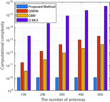
Fig. 4: Variation of the computational complexity vs. the number of antennas.

We proceed to analyze the hardware and software complexities of the proposed joint delay and angle estimation approach. For a large-scale antenna array system using fully digital beamforming, its hardware complexity is $O(N_{\textrm{R}})$. In our proposed approach, the use of the hybrid beamformer allows for a dramatic reduction of the hardware complexity from $O(N_{\textrm{R}})$ to $O(N_{\textrm{RF}})$, where $N_{\textrm{RF}}=\max(N_{\textrm{V}},(2P+1)N_{\textrm{B}})$.

In terms of signal processing complexity, we compare the proposed approach with the state-of-the-art techniques, namely, GBM [2], QRIPM [17], and Q-MLE [21]. For the proposed approach, after hybrid beamforming, the dimension of the received signal is reduced to $N_{\textrm{DS},2}$, so the computational complexity of MDSL processing is $O(N_{\textrm{DS},2}M)=O((2P+1)N_{\textrm{B}}M)=O(\gamma PN_{\textrm{p}}M)$. The computational complexities of calculating the covariance matrix, $\mathbf{R}_{\mathbf{\tilde{\mathbf{y}}}_{\textrm{vec}}}$, in (25) and performing the EVD on $\mathbf{R}_{\mathbf{\tilde{\mathbf{y}}}_{\textrm{vec}}}$ according to (29) are $O(\gamma^{2}P^{2}N_{\textrm{p}}^{2}M^{2}T_{s})$ and $O(\gamma^{3}P^{3}N_{\textrm{p}}^{3}M^{3})$, respectively, where $T_{s}$ is the number of snapshots. The complexities of computing the delay $\hat{\tau}_{l}$ and the elevation angle, $\hat{\theta}_{\mathrm{\textrm{R}},l}$, are $O(MN_{\textrm{p}}^{3})$ and $O(\gamma^{2}N_{\textrm{p}}^{2}+N_{\textrm{p}}^{3})$, respectively. When estimating $\hat{\phi}_{\mathrm{\textrm{R}},l}$ with 1D search using (44), the computational complexity is $O(\gamma^{2}N_{\textrm{p}}^{2}D)$, where $D$ is the size of the search dimension. For the pair matching operation, the computational complexity is $O(N_{\textrm{p}}^{3})$. Thus, the overall computational complexity of our proposed approach is $O(\gamma PN_{\textrm{p}}M+\gamma^{2}P^{2}N_{\textrm{p}}^{2}M^{2}T_{s}+\gamma^{3}P^{3}N_{\textrm{p}}^{3}M^{3}+MN_{\textrm{p}}^{3}+\gamma^{2}N_{\textrm{p}}^{2}+N_{\textrm{p}}^{3}+\gamma^{2}N_{\textrm{p}}^{2}D+N_{\textrm{p}}^{3})$, which does not depend on the number of receive antennas $N_{\textrm{R}}$. The computational complexities of QRIPM and GBM increase rapidly, as the number of receive antennas increases. When the number of receive antennas $N_{\textrm{R}}$ is large, the computational complexities of QRIPM and GBM are $O(N_{\textrm{R}}^{3}M^{4})$ and $O(P^{3}N_{\textrm{V}}^{3}M^{4})$, respectively. The computational complexity of Q-MLE is $O(N_{\textrm{R}}^{2}M^{2}N_{\textrm{AZI}}N_{\textrm{ELE}}N_{\textrm{DEL}}+(N_{\textrm{p}}N_{\textrm{R}}M)^{3.5})$, where $N_{\textrm{AZI}}$, $N_{\textrm{ELE}}$, and $N_{\textrm{DEL}}$ are the search grids of azimuth angle, elevation angle, and delay, respectively.

Fig. 4 compares the computational complexities of the four methods with the growing number of antennas $N_{\textrm{R}}=N_{\textrm{H}}N_{\textrm{V}}$, where $\gamma=2$, $N_{\textrm{p}}=3$, $M=20$, and $P=12$. We set $D=N_{\textrm{AZI}}=N_{\textrm{ELE}}=N_{\textrm{DEL}}=100$. The figure shows that, compared with the existing methods, the proposed approach has a substantially lower computational complexity. The gaps between the proposed algorithm and the existing alternatives are increasingly significant with the growing number of receive antennas at the BS.

V Simulation Results

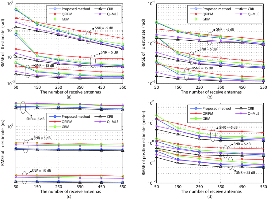
Fig. 5: The RMSE vs. the number of BS antennas for the estimation of different parameters. (a) Azimuth AOA; (b) Elevation AOA; (c) Path delay; and (d) MS position.

In this section, we present simulation results to demonstrate the performance of the proposed approach under different parameters. We set $f_{0}=30$ GHz and $B=2$ GHz, and assume that there are a total of $N_{\textrm{p}}=3$ NLOS paths and $M=20$ consecutive subcarriers. The distance, $h$, between adjacent receiving UCAs and the radius, $r$, of each UCA are $0.5\lambda_{0}$ and $2\lambda_{0}$, respectively.

Fig. 5 plots the root mean square errors (RMSEs) of the estimated angle, delay, and MS position with the increasing number of receive antennas, under different SNR conditions. The proposed algorithm is compared with GBM [2], QRIPM [17], Q-MLE [21], and the Cramér-Rao lower bound (CRLB). Note that GBM [2], QRIPM [17], and Q-MLE [21] are the state of the art for solving the considered parameter estimation problem for UCyAs, and act as the benchmarks in this paper. In particular, the sparsity of the channel is exploited in [2], where the angular space is first discretized and then discrete directions with significant incoming powers are picked up to estimate the channel parameters.

Despite sparse representation techniques were also developed to exploit the sparsity of mmWave multi-antenna systems for channel estimation in [3] and [6], the techniques are not applicable to the problem considered in this paper. One reason is that the sparse representation techniques developed in [3] and [6], based on the DFT of the array steering vectors, are only suitable for ULAs and URAs, where linear recurrence relations exist between the array steering vectors; see [3, eq. (5)] and [6, eq. (3)]. Another reason is that the method developed in [6] only estimates the so-called channel component which is the product of channel parameters (including the channel gain and signal direction), and does not estimate explicitly the channel parameters, e.g., the angle and delay. The method in [3] uses the ML-based algorithms to estimate the channel parameters (i.e., angle and delay) in the same way as Q-MLE [21], which is one of the benchmarks used in our performance evaluation.

As shown in Figs. 5(a) and 5(b), the proposed method and GBM are worse than QRIPM in terms of angle estimation, when the number of antennas is small, i.e., less than 100. The reason is that the proposed algorithm may suffer from an inaccurate approximation in (19), due to the unsatisfied conditions in Theorem 1. However, as the number of antennas increases, the accuracies of the proposed approach and GBM improve faster than that of QRIPM. The proposed method quickly outperforms both QRIPM and GBM, and approaches the CRLB. The improvement slows down with the increasing number of antennas. When the number of antennas is large (e.g., more than 300), the estimation accuracies of the AOAs improve marginally, resulting from the increasingly negligible relative growth of the array aperture of the circular arrays. As also shown in Figs. 5(a) and 5(b), Q-MLE outperforms the other three approaches, including the proposed approach, in terms of angle estimation. However, Q-MLE has a significantly higher computational complexity than the proposed approach, as discussed in Section IV-D.

As shown in Fig. 5(c), the proposed approach achieves the best delay estimation accuracy, attributing to the high temporal resolution of the wideband mmWave signals offered by the MDSI method in the proposed approach. The RMSE curves of the estimated delay appear to be constant. The reason is because the delay estimation precision depends primarily on the signal bandwidth, and is less affected by the number of antennas at the BS (as opposed to the angle estimation). Given its superiority in the angle and delay estimation, the proposed approach outperforms QRIPM, GBM, and Q-MLE in terms of localization, as corroborated in Fig. 5(d).

In order to validate Theorem 1, Fig. 6 plots the RMSE of the angle estimation versus the value of the highest order, $P$, under different numbers of horizontal array response vectors. We see that when the highest order $P\leq 11$, our proposed approach cannot perform satisfactorily, since the number of phase-mode vectors is not sufficient to represent the transformed array response vectors in Section III-B. Fig. 6 also shows that, if $P\geq 12$, for any number of array response vectors, increasing the phase-mode vectors has little influence on the angle estimation performance. This means that the number of phase-mode vectors needed in our approach does not depend on the number of array response vectors, which is important for complexity reduction, as discussed in Section IV-D. In addition, we also see that because the condition in Theorem 1, $N_{\mathrm{H}}\geq 2P$, is unlikely to be satisfied when $N_{\mathrm{H}}=10$, the RMSE is much poorer than those applying more array response vectors.

Fig. 7 assesses statistically the proposed approach by plotting the cumulative distribution function (CDF) of the localization error. We assume that the time offset $\tau_{\textrm{of}}$ obeys a zero-mean Gaussian distribution with the standard deviation of 4 ns, and $\tau_{\textrm{of}}$ is unknown to the BS in the simulation. In Fig. 7(a), we observe that although the performance of the proposed approach decreases with the decline of the average received SNR, the statistical localization error remains small even for SNR = 0 dB, as long as a sufficient number of receive antennas are deployed. In addition, we see that the proposed approach is able to achieve a centimeter-level localization accuracy with a probability of over 60%, when the number of receive antennas is 200. Fig. 7(b) shows the relationship between the localization accuracy and the number of received paths. It can be seen that the proposed approach cannot provide high-accuracy localization with high probability if only a single path is received, since the time offset $\tau_{\textrm{of}}$ is unknown to the BS, as discussed in Section IV-C. In Fig. 7(b), we also see that when the number of received paths is more than three, more paths lead to limited improvement in localization accuracy.

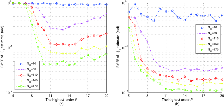
Fig. 6: The RMSE vs. the value of the highest order $P$. (a) The azimuth AOA; and (b) The elevation AOA.

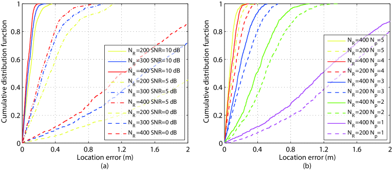
Fig. 7: The CDF of the localization error for different numbers of receive antennas in the case of (a) different received SNR values; and (b) different numbers of received paths

VI Conclusion

In this paper, a novel joint delay and angle estimation approach was proposed for wideband mmWave large-scale hybrid arrays. We proposed a new 3D hybrid beamformer to reduce the number of required RF chains while maintaining the critical recursive property of the space-time response matrix for angle and delay estimation. We also generalized linear interpolation to reconstruct the output signals of the 3D hybrid beamformer and to achieve consistent array response across the wideband and suppress the beam squint effect. As a result, the delay and the azimuth and elevation angles of every multi-path component can be estimated. Simulation results showed that, when a large number of antennas is deployed, our proposed approach is capable of precisely estimating the channel parameters even in low SNR regimes. Potential future extensions of this work include simultaneous localization and environment mapping, performance evaluation of the proposed approach in real-world scenarios, and new techniques to accelerate parameter matching.

Appendix I
Proof of Lemma 1

According to the property of Bessel function, i.e., $J_{-v}(x)=(-1)^{v}J_{v}(x)$, we have $\left|J_{-v}(x)\right|=\left|J_{v}(x)\right|$, so here we only use $J_{v}(x)$ with $v\in\mathbb{Z}^{+}$ for illustration convenience. Let $x=v\rho,\rho\in(0,1]$. The Bessel function, $J_{v}(x)$, whose order $v$ exceeds its argument, $x$, can be written in the following form [32]

$$J_{v}(v\rho)=\frac{1}{\pi}\int_{0}^{\pi}\exp\left(-vF(\vartheta,\rho)\right)d\vartheta,$$ (49)

where

$$F(\vartheta,\rho) =\log\left(\frac{\vartheta+\sqrt{\vartheta^{2}-\rho^{2}\sin^{2}\vartheta}}{\rho\sin\vartheta}\right)$$

$$-\cot\vartheta\sqrt{\vartheta^{2}-\rho^{2}\sin^{2}\vartheta}.$$

The partial derivative of (49) with respect to $\rho$ is calculated as

$$\frac{\partial}{\partial\rho}J_{v}(v\rho)=-\frac{v}{\pi}\int_{0}^{\pi}\frac{\partial F(\vartheta,\rho)}{\partial\rho}\exp\left(-vF(\vartheta,\rho)\right)d\vartheta$$

$$=\frac{v}{\pi\rho}\int_{0}^{\pi}g(\vartheta,\rho)\exp\left(-vF(\vartheta,\rho)\right)d\vartheta,$$ (50)

where $g(\vartheta,\rho)=\left(\vartheta-\rho^{2}\sin\vartheta\cos\vartheta\right)/\sqrt{\vartheta^{2}-\rho^{2}\sin^{2}\vartheta}.$ Considering that

$$g(\vartheta,\rho) =\frac{\vartheta-\rho^{2}\sin\vartheta\cos\vartheta}{\sqrt{\vartheta^{2}-\rho^{2}\sin^{2}\vartheta}}\geq\frac{\vartheta-\sin\vartheta\cos\vartheta}{\sqrt{\vartheta^{2}-\rho^{2}\sin^{2}\vartheta}}$$

$$\geq\frac{\vartheta-\sin\vartheta}{\sqrt{\vartheta^{2}-\rho^{2}\sin^{2}\vartheta}}\geq 0,$$ (51)

we have $\partial J_{v}(v\rho)/\partial\rho>0,$ and conclude that $J_{v}(v\rho)$ is a positive increasing function of $\rho$. Thus, $J_{v}(v\rho)<J_{v}(v).$

On the other hand, the partial derivative of (49) with respect to $v$ is calculated as

$$\frac{\partial}{\partial v}J_{v}(v\rho)=-\frac{1}{\pi}\int_{0}^{\pi}F(\vartheta,\rho)\exp\left(-vF(\vartheta,\rho)\right)d\vartheta.$$ (52)

Because

$$\frac{\partial}{\partial\vartheta}F(\vartheta,\rho)=\frac{(1-\rho\cot\vartheta)^{2}}{\sqrt{\vartheta^{2}-\rho^{2}\sin^{2}\vartheta}}+\sqrt{\vartheta^{2}-\rho^{2}\sin^{2}\vartheta}\geq 0$$ (53)

and $\partial F(0,\rho)/\partial\rho=-\sqrt{1-\rho^{2}}/\rho\leq 0$, we have $F(\vartheta,\rho)\geq F(0,\rho)\geq F(0,1)=0$, and hence $\partial J_{v}(v\rho)/\partial v<0$. This means that $J_{v}(v\rho)$ is a positive decreasing function of $v$, i.e., $J_{v}(v\rho)\leq J_{1}(\rho).$ Therefore, we have $J_{v}(v\rho)<J_{v}(v)\leq J_{1}(1)\approx 0.44$ with $\rho\in(0,1]$ and $v\in\mathbb{Z}^{+}$. When $\left|v\right|>\left|x\right|$, $\left|J_{v}(x)\right|\approx 0,\>v\in\mathbb{Z}.$

Appendix II
Proof of Theorem 1

According to Lemma 1, we observe that $J_{p}(\varpi_{m,l})$ cannot be omitted if $\left|p\right|\leq\left|\varpi_{m,l}\right|=\left|2\pi f_{m}r\sin(\theta_{\textrm{R},l})/c\right|\leq 2\pi f_{m}r/c$. Because $f_{0}\leq f_{m}$ and $p\in\mathbb{Z}$, we set the highest order $P=\max(\left|p\right|)=\left\lfloor 2\pi f_{0}r/c\right\rfloor$.

On the other hand, in the case of $Q\neq 0$, because $p\in[-P,P]\cap\mathbb{Z}$ and $N_{\mathrm{H}}\geq 2P$, we have $\left|p-QN_{\mathrm{H}}\right|\geq\left|\varpi_{m,l}\right|$. According to Lemma 1, we obtain

$$\left|\varepsilon_{p,Q}(\varpi_{m,l},\phi_{\textrm{R},l})\right|$$

$$=\left|j^{(QN_{\mathrm{H}}-p)}J_{(QN_{\mathrm{H}}-p)}(\varpi_{m,l})\exp\left(j(QN_{\mathrm{H}}-p)\phi_{\textrm{R},l}\right)\right|$$

$$=\left|J_{(p-QN_{\mathrm{H}})}(\varpi_{m,l})\right|\approx 0.$$ (54)

In this case, (14) can be approximated by

$$A_{\textrm{PM},p} =\sqrt{N_{\textrm{H}}}\left[j^{p}J_{p}(\varpi_{m,l})e^{-jp\phi_{\textrm{R},l}}\vphantom{\sum_{Q\neq 0}^{\infty}}\right.$$

$$\left.+\sum_{Q=-\infty,Q\neq 0}^{\infty}\varepsilon_{p,Q}(\varpi_{m,l},\phi_{\textrm{R},l})\right]$$

$$\approx\sqrt{N_{\textrm{H}}}j^{p}J_{p}(\varpi_{m,l})e^{-jp\phi_{\textrm{R},l}}.$$ (55)

This concludes the proof of Theorem 1.

Zhipeng Lin (M’20) is currently working toward the dual Ph.D. degrees in communication and information engineering in the School of Information and Communication Engineering, Beijing University of Posts and Telecommunications, Beijing, China, and the School of Electrical and Data Engineering, University of Technology of Sydney, NSW, Australia. His current research interests include millimeter-wave communication, massive MIMO, hybrid beamforming, wireless localization, and tensor processing.

Tiejun Lv (M’08-SM’12) received the M.S. and Ph.D. degrees in electronic engineering from the University of Electronic Science and Technology of China (UESTC), Chengdu, China, in 1997 and 2000, respectively. From January 2001 to January 2003, he was a Postdoctoral Fellow with Tsinghua University, Beijing, China. In 2005, he was promoted to a Full Professor with the School of Information and Communication Engineering, Beijing University of Posts and Telecommunications (BUPT). From September 2008 to March 2009, he was a Visiting Professor with the Department of Electrical Engineering, Stanford University, Stanford, CA, USA. He is the author of 3 books, more than 80 published IEEE journal papers and 190 conference papers on the physical layer of wireless mobile communications. His current research interests include signal processing, communications theory and networking. He was the recipient of the Program for New Century Excellent Talents in University Award from the Ministry of Education, China, in 2006. He received the Nature Science Award in the Ministry of Education of China for the hierarchical cooperative communication theory and technologies in 2015.

Wei Ni (M’09-SM’15) received the B.E. and Ph.D. degrees in Electronic Engineering from Fudan University, Shanghai, China, in 2000 and 2005, respectively. Currently, he is a Group Leader and Principal Research Scientist at CSIRO, Sydney, Australia, and an Adjunct Professor at the University of Technology Sydney and Honorary Professor at Macquarie University, Sydney. He was a Postdoctoral Research Fellow at Shanghai Jiaotong University from 2005 – 2008; Deputy Project Manager at the Bell Labs, Alcatel/Alcatel-Lucent from 2005 to 2008; and Senior Researcher at Devices R&D, Nokia from 2008 to 2009. His research interests include signal processing, stochastic optimization, learning, as well as their applications to network efficiency and integrity. Dr Ni is the Chair of IEEE Vehicular Technology Society (VTS) New South Wales (NSW) Chapter since 2020 and an Editor of IEEE Transactions on Wireless Communications since 2018. He served first the Secretary and then Vice-Chair of IEEE NSW VTS Chapter from 2015 to 2019, Track Chair for VTC-Spring 2017, Track Co-chair for IEEE VTC-Spring 2016, Publication Chair for BodyNet 2015, and Student Travel Grant Chair for WPMC 2014.

J. Andrew Zhang (M’04-SM’11) received the B.Sc. degree from Xi’an JiaoTong University, China, in 1996, the M.Sc. degree from Nanjing University of Posts and Telecommunications, China, in 1999, and the Ph.D. degree from the Australian National University, in 2004. Currently, Dr. Zhang is an Associate Professor in the School of Electrical and Data Engineering, University of Technology Sydney, Australia. He was a researcher with Data61, CSIRO, Australia from 2010 to 2016, the Networked Systems, NICTA, Australia from 2004 to 2010, and ZTE Corp., Nanjing, China from 1999 to 2001. Dr. Zhang’s research interests are in the area of signal processing for wireless communications and sensing. He has published more than 180 papers in leading international Journals and conference proceedings, and has won 5 best paper awards. He is a recipient of CSIRO Chairman’s Medal and the Australian Engineering Innovation Award in 2012 for exceptional research achievements in multi-gigabit wireless communications.

Jie Zeng (M’09–SM’16) received the B.S. and M.S. degrees from Tsinghua University in 2006 and 2009, respectively, and received the Ph.D. degree from Beijing University of Posts and Telecommunications in 2019. From 2009, he has been with Tsinghua University. His research interests include 5G, IoT, URLLC, novel multiple access, and novel network architecture. He has authored three books related to 5G, has published over 100 journal and conference papers, and holds more than 30 Chinese and international patents. He participated in drafting one national standard and one communication industry standard in China. He received the science and technology award of Beijing in 2015 and the best cooperation award of Samsung Electronics in 2016.

Ren Ping Liu (M’09-SM’14) received his B.E. and M.E. degrees from Beijing University of Posts and Telecommunications, China, and the Ph.D. degree from the University of Newcastle, Australia. He is currently a Professor and Head of Discipline of Network & Cybersecurity at University of Technology Sydney. Professor Liu was the co-founder and CTO of Ultimo Digital Technologies Pty Ltd, developing IoT and Blockchain. Prior to that he was a Principal Scientist and Research Leader at CSIRO, where he led wireless networking research activities. He specialises in system design and modelling and has delivered networking solutions to a number of government agencies and industry customers. His research interests include wireless networking, Cybersecurity, and Blockchain. Professor Liu was the founding chair of IEEE NSW VTS Chapter and a Senior Member of IEEE. He served as Technical Program Committee chairs and Organising Committee chairs in a number of IEEE Conferences. Prof Liu was the winner of Australian Engineering Innovation Award and CSIRO Chairman medal. He has over 200 research publications.

References

• [1] E. Hossain, M. Rasti, H. Tabassum, and A. Abdelnasser, “Evolution towards 5G multi-tier cellular wireless networks: An interference management perspective,” IEEE Wireless Commun. Mag., vol. 21, no. 3, pp. 118–127, Jun. 2014.
• [2] Z. Lin, T. Lv, and P. T. Mathiopoulos, “3-D indoor positioning for millimeter-Wave massive MIMO systems,” IEEE Trans. Commun., vol. 66, no. 6, pp. 2472–2486, June 2018.
• [3] A. Shahmansoori, G. E. Garcia, G. Destino, et al., “Position and orientation estimation through millimeter-wave MIMO in 5G systems,” IEEE Trans. Wireless Comm., vol. 17, no. 3, pp. 1822–1835, Mar. 2018.
• [4] T. Rappaport, S. Sun, R. Mayzus, et al., “Millimeter wave mobile communications for 5G cellular: It will work!,” IEEE Access, vol. 1, pp. 335–349, May 2013.
• [5] Z. Lin, T. Lv, J. A. Zhang, and R. P. Liu, “3D wideband mmWave localization for 5G massive MIMO systems,” in Proc. IEEE Globecom, Waikoloa, HI, USA, Dec. 2019, pp. 1033–1038.
• [6] X. Gao, L. Dai, S. Han, C. Lin I, and X. Wang, “Reliable beamspace channel estimation for millimeter-wave massive MIMO systems with lens antenna array,” IEEE Trans. Wireless Commun., vol. 16, no. 9, pp. 6010–6021, Sep. 2017.
• [7] L. Zhu and J. Zhu, “Optimal design of uniform circular antenna array in mmWave LOS MIMO channel,” IEEE Access, vol. 6, pp. 61022–61029, Sep. 2018.
• [8] P. Wang, Y. Li, and B. Vucetic, “Millimeter wave communications with symmetric uniform circular antenna arrays,” IEEE Commun. Letters, vol. 18, no. 8, pp. 1307–1310, Aug. 2014.
• [9] J. A. Zhang, X. Huang, V. Dyadyuk, et al., “Massive hybrid antenna array for millimeter-wave cellular communications,” IEEE Wireless Commun., vol. 22, no. 1, pp. 79–87, Feb. 2015.
• [10] R. W. Heath Jr., N. G. Prelcic, S. Rangan, et al., “An overview of signal processing techniques for millimeter wave MIMO systems,” IEEE J. Sel. Topics Signal Process., vol. 10, no. 3, pp. 436–453, Apr. 2016.
• [11] Z. Lin, T. Lv, W. Ni, J. A. Zhang, and R. P. Liu, “Tensor-based multi-dimensional wideband channel estimation for mmWave hybrid cylindrical arrays,” IEEE Trans. Commun., pp. 1–15, Sep. 2020.
• [12] A. Alkhateeb, O. E. Ayach, G. Leus, et al., “Channel estimation and hybrid precoding for millimeter wave cellular systems,” IEEE J. Sel. Topics Signal Process., vol. 8, no. 5, pp. 831–846, Oct. 2014.
• [13] A. Liao, Z. Gao, Y. Wu, et al., “2D unitary ESPRIT based super-resolution channel estimation for millimeter-wave massive MIMO with hybrid precoding,” IEEE Access, vol. 5, pp. 24747–24757, Nov. 2017.
• [14] T. Trump and B. Ottersten, “Estimation of nominal direction of arrival and angular spread using an array of sensors,” Signal Process., vol. 50, no. 1-2, pp. 57–69, Apr. 1996.
• [15] R. O. Schmidt, “Multiple emitter location and signal parameter estimation,” IEEE Trans. Antennas Propag., vol. 34, no. 3, pp. 276–280, Jul. 1986.
• [16] R. Roy, A. Paulraj, and T. Kailath, “ESPRIT-a subspace rotation approach to estimation of parameters of cisoids in noise,” IEEE Trans. Acoust. Speech Signal Process., vol. 34, no. 5, pp. 1340–1342, Oct. 1986.
• [17] X. Guo, Q. Wan, X. Shen, et al., “Low-complexity parameters estimator for multiple 2D domain incoherently distributed sources,” Turk. J. Elect. Eng. Comput. Sci., vol. 3, no. 19, pp. 445–462, May 2011.
• [18] N. D. Sidiropoulos, R. Bro, and G. B. Giannakis, “Parallel factor analysis in sensor array processing,” IEEE Trans. Signal Process., vol. 48, no. 8, pp. 2377–2388, Aug. 2000.
• [19] J. H. Brady and A. M. Sayeed, “Wideband communication with high-dimensional arrays: New results and transceiver architectures,” in Proc. IEEE Int. Conf. Commun. Workshop (ICCW), London, U.K., Jun. 2015, pp. 1042–1047.
• [20] Z. Lin, T. Lv, W. Ni, J. A. Zhang, and R. P. Liu, “Nested hybrid cylindrical array design and DoA estimation for massive IoT networks,” IEEE J. Sel. Areas Commun., pp. 1–15, Aug. 2020.
• [21] Baldur Steingrimsson, Zhi-Quan Luo, and Kon Max Wong, “Soft quasi-maximum-likelihood detection for multiple antenna wireless channels,” IEEE Trans. Signal Process., vol. 51, no. 11, pp. 2710–2718, Nov. 2003.
• [22] B. D. Van Veen and K. M. Buckley, “Beamforming: A versatile approach to spatial filtering,” IEEE Acoust. Speech Sig. Proc. Mag., vol. 5, no. 5, pp. 4–24, Apr. 1988.
• [23] F. Raimondi, P. Comon, and O. Michel, “Wideband multilinear array processing through tensor decomposition,” in Proc. IEEE Int. Conf. Acoust. Speech Signal Process. (ICASSP), Shanghai, China, Mar. 2016, pp. 2951–2955.
• [24] L. Zou, J. Lasenby, and Z. He, “Direction and polarisation estimation using polarised cylindrical conformal arrays,” IET Signal Process., vol. 6, no. 5, pp. 395–403, July 2012.
• [25] T. Lv, F. Tan, H. Gao, et al., “A beamspace approach for 2-D localization of incoherently distributed sources in massive MIMO systems,” Signal Process., vol. 121, pp. 30–45, Apr. 2016.
• [26] Xuan Hui Wu, Mohamed Yehia, and Ahmed Abdalla, “A cylindrical antenna array for mimo radar applications,” in Proc. IEEE Int. Symp. Ant. Propag. (APSURSI), Memphis, TN, USA, July 2014, pp. 484–485.
• [27] V. Liepins, “Extended Fourier analysis of signals,” Mar. 2013, arXiv:1303.2033.
• [28] X. Gao, L. Dai, S. Han, et al., “Energy-efficient hybrid analog and digital precoding for mmwave MIMO systems with large antenna arrays,” IEEE J. Sel. Areas Commun., vol. 34, no. 4, pp. 998–1009, April 2016.
• [29] M.-T. Martinez-Ingles, D. Gaillot, J. Pascual-Garcia, et al., “Deterministic and experimental indoor mmW channel modeling,” IEEE Ant. Wireless Prop. Lett., vol. 13, pp. 1047–1050, May 2014.
• [30] Mathew K. Samimi and Theodore S. Rappaport, “3-D millimeter-wave statistical channel model for 5G wireless system design,” IEEE Trans. Microw. Theory Techn., vol. 64, no. 7, pp. 2207–2225, July 2016.
• [31] Alain Olivier, Guillermo Bielsa, Irene Tejado, et al., “Lightweight indoor localization for 60-GHz millimeter wave systems,” in Proc. IEEE Int. Symp. Ant. Propag. (APSURSI), London, UK, Jun. 2016, pp. 1–9.
• [32] G. N. Watson, A Treatise on the Theory of Bessel Functions, Cambridge Univ. Press, Cambridge, U.K., 2nd edition, 1952.
• [33] R. J. Mailloux, Phased Array Antenna Handbook, Artech House, Norwood, United States, 2nd edition, 2005.
• [34] C. E. Shannon, “Communication in the presence of noise,” Proceedings of the IRE, vol. 37, no. 1, pp. 10–21, Jan. 1949.
• [35] J. Zhang, I. Podkurkov, M. Haardt, et al., “Efficient multidimensional parameter estimation for joint wideband radar and communication systems based on OFDM,” in Proc. IEEE Int. Conf. Acoust. Speech Signal Process. (ICASSP), New Orleans, LA, USA, Mar. 2017, pp. 3091–3100.
• [36] M. C. Vanderveen, A. J. van der Veen, and A. Paulraj, “Estimation of multipath parameters in wireless communications,” IEEE Trans. Signal Process., vol. 46, no. 3, pp. 682–690, Mar. 1998.
• [37] A. Hu, T. Lv, H. Gao, et al., “An ESPRIT-based approach for 2-D localization of incoherently distributed sources in massive MIMO systems,” IEEE J. Sel. Topics Signal Process., vol. 8, no. 5, pp. 996–1011, Oct. 2014.
• [38] A. J. van der Veen, P.B. Ober, and E.F. Deprettere, “Azimuth and elevation computation in high resolution DOA estimation,” IEEE Trans. Signal Process., vol. 40, no. 7, pp. 1828–1832, July 1992.
• [39] A. L. Swindlehurst and T. Kailath, “Azimuth/elevation direction finding using regular array geometrics,” IEEE Aerosp. Electron. Syst., vol. 29, no. 1, pp. 145–156, Jan. 1993.
• [40] Hiroshi Kawasaki, Yuuki Horita, Hiroki Morinaga, et al., “Structured light with coded aperture for wide range 3D measurement,” in Proc. IEEE Int. Conf. Image Process. (ICIP), Orlando, FL, USA, Oct. 2012, pp. 2777–2780.
• [41] Bisheng Yang and Yufu Zang, “Automated registration of dense terrestrial laser-scanning point clouds using curves,” ISPRS J. Photogrammetry Remote Sensing, vol. 95, pp. 109–121, Sep. 2014.
• [42] D. Wang, M. Fattouche, and X. Zhan, “Pursuance of mm-level accuracy: Ranging and positioning in mmWave systems,” IEEE Systems J., vol. PP, no. 99, pp. 1–12, Mar. 2018.