Background Field Method and Generalized Field Redefinitions
in Effective Field Theories.

A. Quadri andrea.quadri@mi.infn.it INFN, Sezione di Milano, via Celoria 16, I-20133 Milano, Italy
(February 21, 2021)
Abstract

We show that in a spontaneously broken effective gauge field theory, quantized in a general background $R_{\xi}$-gauge, also the background fields undergo a non-linear (albeit background-gauge invariant) field redefinition induced by radiative corrections. This redefinition proves to be crucial in order to renormalize the coupling constants of gauge-invariant operators in a gauge-independent way. The classical background-quantum splitting is also in general non-linearly deformed (in a non gauge-invariant way) by radiative corrections. Remarkably, such deformations vanish in the Landau gauge, to all orders in the loop expansion.

pacs:
11.10.Gh, 12.60.-i, 12.60.Fr

I Introduction

In the absence of direct resonance signals of new physics beyond the Standard Model (BSM) at the LHC, indirect experimental searches of BSM physics have become increasingly popular in recent years, e.g. lepton flavour universality violations  Aaij et al. (2014, 2016); Sirunyan et al. (2018); Aaboud et al. (2018) or searches for non-resonant Higgs boson pair production (for a recent review see Guerrero (2021)).

In this context the SM Effective Field Theory (SMEFT) Buchmuller and Wyler (1986); Grzadkowski et al. (2010); Brivio and Trott (2019) provides a consistent theoretical tool in order to describe the energy regime up to some higher energy scale $\Lambda$. The advantage of the SMEFT is that it takes into account the constraints arising from the invariance under the $\rm SU(3)\times SU_{L}(2)\times U_{Y}(1)$ gauge group in a model independent way, without the need to know the precise form of its ultraviolet (UV) completion.

In this approach the SM Lagrangian is supplemented by higher dimensional gauge-invariant operators suppressed by powers of $\Lambda$. Renormalizability by power-counting is then lost and new UV divergences arise order by order in the loop expansion. As in any effective gauge theory, they must be subtracted by a combination of generalized (i.e. non-linear and in general not even polynomial Binosi and Quadri (2019)) field redefinitions and the renormalization of the coupling constants, associated with gauge-invariant operators of increasing dimensions Anselmi (2013); Gomis and Weinberg (1996).

That such a program can indeed be completed in a recursive way by adding local counter-terms while preserving the relevant symmetries of the theory is a key result established many years ago Gomis and Weinberg (1996) in the setting of the Batalin-Vilkovisky (BV) formalism (for a review see e.g. Gomis et al. (1995)).

The BV formalism can be seen as a generalization of the BRST quantization procedure Becchi et al. (1974, 1975, 1976) that applies also to non power-counting renormalizable models. The Slavnov-Taylor (ST) identity Slavnov (1972); Taylor (1971), encoding at the quantum level the BRST invariance of the classical gauge-fixed action, is translated into the BV master equation.

From a physical point of view the BV master equation ensures, as well as the ST identity, physical unitarity of the theory, i.e. the cancellation of unphysical ghosts in the intermediate states Becchi et al. (1974); Kugo and Ojima (1978); Curci and Ferrari (1976); Ferrari and Quadri (2004).

Due to the huge number of operators arising in effective field theories it is natural to apply the background field method (BFM) DeWitt (1967); Kluberg-Stern and Zuber (1975); Boulware (1981); Hart (1983); Abbott (1981); Abbott et al. (1983); Ichinose and Omote (1982); Capper and MacLean (1982); Denner et al. (1995, 1996); Grassi (1999, 1996); Becchi and Collina (1999); Ferrari et al. (2001) technique in order to simplify the task of computing the radiative corrections. The BFM is particularly advantageous since it allows to retain (background) gauge invariance to all orders in perturbation theory. The resulting background Ward identity is linear in the quantum fields, unlike the ST identity, and hence is easier to study. Use of the BFM has been recently advocated in the context of the (geometric) SMEFT in Refs Helset et al. (2018); Corbett et al. (2020); Corbett and Trott (2020).

In power-counting renormalizable theories both the background and the quantum fields renormalize linearly. Linearity of the renormalization of the background fields together with background gauge invariance yields powerful relations between counter-terms that are one of the main virtues of the BFM Weinberg (2013).

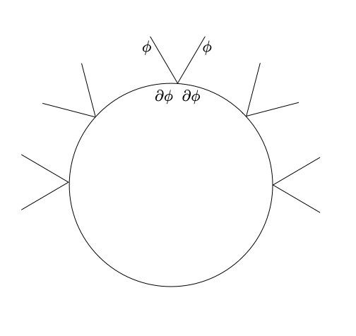
The situation is significantly more involved in effective gauge theories. For instance a typical derivative-dependent dim.6 interaction $\sim(\phi\partial\phi)^{2}$ gives rise already at one loop to an infinite number of UV-divergent amplitudes, generated by configurations with two powers of the internal loop momentum from the derivative-dependent interaction at each vertex. They are compensated by two inverse powers from each propagator (see Figure 1), so that the UV degree of divergence of these Feynman amplitudes is always $4$, irrespectively of the number of the external $\phi$-legs.

Refer to caption
Figure 1: Maximally UV divergent one-loop amplitudes generated by the vertex $(\phi\partial\phi)^{2}$

The task of evaluating the required counter-terms in spontaneously broken effective gauge field theories is simplified in the so-called $X$-formalism Quadri (2006, 2017); Binosi and Quadri (2018) by the use of a gauge-invariant field coordinate for the physical scalar mode, namely $X_{2}\sim\frac{1}{v}\Big{(}\phi^{\dagger}\phi-\frac{v^{2}}{2}\Big{)}$, where $\phi$ is the usual Higgs doublet and $v$ its vacuum expectation value (v.e.v.).

Let us consider e.g. the two-derivatives vertices $(\phi\partial\phi)^{2}$ arising from the gauge-invariant interaction $\Big{(}\phi^{\dagger}\phi-\frac{v^{2}}{2}\Big{)}(D^{\mu}\phi)^{\dagger}D_{\mu}\phi\,,$ $D_{\mu}$ being the covariant derivative. This operator is represented in the $X$-formalism by $\sim X_{2}(D^{\mu}\phi)^{\dagger}D_{\mu}\phi\,$ Binosi and Quadri (2019). Since the $X_{2}$-amplitudes are uniquely fixed by the functional identities of the theory Binosi and Quadri (2019), one needs to consider only graphs with internal $X_{2}$-lines, so that at least one derivative acts on the external $\phi$-legs, thus reducing the UV degree of divergence of the amplitudes that need to be evaluated. There is only a finite number of UV divergent amplitudes of this type, so one can renormalize this sector of the theory by a finite number of independent (i.e. not fixed by the symmetries) local counter-terms, while diagrams in Figure 1 are automatically taken into account by an algebraic resummation induced by the functional identities of the model Quadri (2006, 2017); Binosi and Quadri (2018).

In effective gauge theories quantum fields undergo generalized non-linear field redefinitions (GFRs). The $X$-formalism provides an effective way to separate the renormalization of the gauge coupling constants from the physically spurious contributions controlled by the GFRs Quadri (2006, 2017); Binosi and Quadri (2018). GFRs play a crucial role in carrying out the correct recursive off-shell renormalization of the one-particle-irreducible (1-PI) amplitudes, since only once the appropriate GFRs have been implemented, the renormalization of the coupling constants turns out to be gauge-independent Binosi and Quadri (2020a, 2019, b).

When effective gauge theories are quantized in the BFM, the question arises of whether also the background fields undergo a non-linear redefinitions, and if such a redefinition is background gauge-invariant.

This is a non trivial issue that can be studied by combining the $X$-formalism with the Algebraic Renormalization approach to the BFM Ferrari et al. (2001); Becchi and Collina (1999); Grassi (1999, 1996). Compatibilty between the ST identity and the background Ward identity is obtained by extending the BRST differential $s$ to the background fields, collectively denoted by $\widehat{\Phi}$, and by pairing them with anticommuting variables $\Omega_{\widehat{\Phi}}$, so that

$\displaystyle s\widehat{\Phi}=\Omega_{\widehat{\Phi}}\,,\qquad s\Omega_{\widehat{\Phi}}=0\,.$ (1)

The corresponding extended ST identity uniquely fixes (in a background gauge-invariant way) the dependence of the vertex functional on the background fields $\widehat{\Phi}$.

In the present paper we extend the $X$-formalism to the BFM and study the renormalization of the Abelian Higgs-Kibble model supplemented by dim.6 operators, as a playground towards the renormalization of the SMEFT in the BFM approach.

We find that:

  1. 1.

    the tree-level background-quantum splitting

    $$\Phi=\widehat{\Phi}+Q_{\Phi}$$

    is in general deformed in a non-linear (and gauge-dependent) way, unlike in the power-counting renormalizable case where only multiplicative $Z$-factors arise both for background and quantum fields;

  2. 2.

    a noticeable exception is the Landau gauge, where no such deformation of the tree-level background-quantum splitting happens, to all orders in the loop expansion;

  3. 3.

    as a consequence of the radiative corrections to the background-quantum splitting and of the GFRs, background fields also undergo a non-linear redefinition;

  4. 4.

    the redefinition of the background fields is background gauge-invariant. This result follows from non-trivial cancellations between the non gauge-invariant contributions to the background-quantum splitting and the non gauge-invariant terms in the GFRs;

  5. 5.

    the background and quantum field redefinitions are crucial in order to properly renormalize the coupling constants in a gauge-independent way.

The paper is organized as follows. In Sect. II we set up our notations, present the classical action of the Abelian Higgs-Kibble model with dim.6 operators in the $X$-formalism and introduce the BFM tree-level vertex functional, together with the background gauge-fixing. In Sect. III we study the compatibility between the background Ward identity and the mapping from the $X$-formalism to the standard $\phi$-representation (target theory). We prove that 1-PI amplitudes in the target theory are background gauge-invariant if those in the $X$-theory are. In Sect. IV we study the local solutions to the background Ward identity that are relevant for the classification of the UV divergences of the theory. In Sect. V we solve the ST identity in order to fix the dependence on the background fields. We find that the tree-level background-quantum splitting is non-trivially deformed at the quantum level. The gauge dependence of such corrections is studied in the Feynman and in the Landau gauge. In Sect. VI we obtain the generalized field and background redefinitions for the $X$-theory by combining the effect of the deformation of the background-quantum splitting and of the GFRs. As a non-trivial check, we show that at zero quantum fields $Q_{\Phi}=0$ subtle cancellations happen that make the vertex functional invariant w.r.t. the background transformation of the background fields only, in agreement with the background Ward identity. Finally in Sect. VII we provide the explicit form of the GFRs both for background and quantum fields in the ordinary $\phi$-formalism by applying the mapping from the $X$- to the target theory. Conclusions are presented in Sect. VIII.

Appendices contain the discussions of some aspects of the Algebraic Renormalization of the theory. In Appendix A we enumerate the functional symmetries of the model. Appendix B is devoted to the parameterization of background gauge field redefinitions. The renormalization of the tadpole and its gauge dependence are studied in Appendix C.

II BFM tree-level vertex functional

We start from the tree-level vertex functional of the Abelian Higgs-Kibble model supplemented by dim.6 gauge-invariant operators in the so-called $X$-formalism of Binosi and Quadri (2020b):

$\displaystyle\Gamma^{(0)}$ $\displaystyle=\int\!\mathrm{d}^{4}x\,\Big{[}-\frac{1}{4}F^{\mu\nu}F_{\mu\nu}+(D^{\mu}\phi)^{\dagger}(D_{\mu}\phi)-\frac{M^{2}-m^{2}}{2}X_{2}^{2}-\frac{m^{2}}{2v^{2}}\Big{(}\phi^{\dagger}\phi-\frac{v^{2}}{2}\Big{)}^{2}$
$\displaystyle-\bar{c}(\square+m^{2})c+\frac{1}{v}(X_{1}+X_{2})(\square+m^{2})\Big{(}\phi^{\dagger}\phi-\frac{v^{2}}{2}-vX_{2}\Big{)}$
$\displaystyle+\frac{z}{2}\partial^{\mu}X_{2}\partial_{\mu}X_{2}+\frac{g_{1}v}{\Lambda^{2}}X_{2}(D^{\mu}\phi)^{\dagger}(D_{\mu}\phi)+\frac{g_{2}v}{\Lambda^{2}}X_{2}F_{\mu\nu}^{2}+\frac{g_{3}v^{3}}{6\Lambda^{2}}X_{2}^{3}$
$\displaystyle+T_{1}(D^{\mu}\phi)^{\dagger}(D_{\mu}\phi)+UF_{\mu\nu}^{2}+RX_{2}^{2}$
$\displaystyle+\frac{\xi b^{2}}{2}-b\Big{(}\partial A+\xi ev\chi\Big{)}+\bar{\omega}\Big{(}\square\omega+\xi e^{2}v(\sigma+v)\omega\Big{)}$
$\displaystyle+\bar{c}^{*}\Big{(}\phi^{\dagger}\phi-\frac{v^{2}}{2}-vX_{2}\Big{)}+\sigma^{*}(-e\omega\chi)+\chi^{*}e\omega(\sigma+v)\Big{]}.$ (2)

The field content of the model includes the Abelian gauge field $A_{\mu}$, the usual scalar field

$$\phi\equiv\frac{1}{\sqrt{2}}(\phi_{0}+i\chi)=\frac{1}{\sqrt{2}}(\sigma+v+i\chi)\,,\qquad\phi_{0}=\sigma+v\,,$$

with $v$ denoting the v.e.v., and a singlet field $X_{2}$ describing in a gauge invariant way the physical scalar mode of mass $M$. Indeed, if one goes on-shell in Eq.(2) with the auxiliary field $X_{1}$, that plays the role of a Lagrange multiplier, we obtain the constraint

$$(\square+m^{2})\Big{(}\phi^{\dagger}\phi-\frac{v^{2}}{2}-vX_{2}\Big{)}=0,$$

so that the field $X_{2}$ must fulfill the condition $X_{2}=\frac{1}{v}\Big{(}\phi^{\dagger}\phi-\frac{v^{2}}{2}\Big{)}+\eta,$ $\eta$ being a scalar field of mass $m$. However, it can be proven that in perturbation theory the correlators of the mode $\eta$ with any gauge-invariant operators vanish Binosi and Quadri (2019), so that one can safely set $\eta=0$ and by going on-shell perform in Eq. (2) the substitution

$$X_{2}\sim\frac{1}{v}(\phi^{\dagger}\phi-v^{2}/2)\,.$$

The $m^{2}$-term cancels out and one gets back the usual Higgs quartic potential with coefficient $\sim M^{2}/2v^{2}$ plus the set of dim.6 parity-preserving operators arising from the third line of Eq.(2) (we use the same notations as in Binosi and Quadri (2020a)):

$\displaystyle{\cal O}_{1}^{[6]}$ $\displaystyle=\int\!\mathrm{d}^{4}x\,\,F_{\mu\nu}^{2}\Big{(}\phi^{\dagger}\phi-\frac{v^{2}}{2}\Big{)}\sim\int\!\mathrm{d}^{4}x\,\,vX_{2}F_{\mu\nu}^{2},$ (3a)
$\displaystyle{\cal O}_{2}^{[6]}$ $\displaystyle=\int\!\mathrm{d}^{4}x\,\,\Big{(}\phi^{\dagger}\phi-\frac{v^{2}}{2}\Big{)}^{3}\sim\int\!\mathrm{d}^{4}x\,\,v^{3}X_{2}^{3},$ (3b)
$\displaystyle{\cal O}_{3}^{[6]}$ $\displaystyle=\int\!\mathrm{d}^{4}x\,\,\Big{(}\phi^{\dagger}\phi-\frac{v^{2}}{2}\Big{)}\square\Big{(}\phi^{\dagger}\phi-\frac{v^{2}}{2}\Big{)}\sim\int\!\mathrm{d}^{4}x\,\,v^{2}X_{2}\square X_{2},$ (3c)
$\displaystyle{\cal O}_{4}^{[6]}$ $\displaystyle=\int\!\mathrm{d}^{4}x\,\,\Big{(}\phi^{\dagger}\phi-\frac{v^{2}}{2}\Big{)}(D^{\mu}\phi)^{\dagger}D_{\mu}\phi\sim\int\!\mathrm{d}^{4}x\,\,vX_{2}(D^{\mu}\phi)^{\dagger}D_{\mu}\phi.$ (3d)

We notice that the parameter $m^{2}$ must disappear in the correlators of the gauge-invariant operators of the target theory (i.e. the one obtained by going on-shell with the $X_{1,2}$-fields), as can be checked explicitly at the one loop order Binosi and Quadri (2019, 2020a, 2020b, 2018).

In Eq.(2) $\bar{\omega},\omega$ are the Faddeev-Popov antighost and ghost fields, while $b$ is the Nakanishi-Lautrup field enforcing the gauge-fixing condition

$${\cal F}_{\xi}=0$$

with

$\displaystyle{\cal F}_{\xi}\equiv\partial A+\xi ev\chi\,,$ (4)

$\xi$ being the gauge parameter.

The tree-level vertex functional (2) is invariant both under the usual gauge BRST symmetry

$\displaystyle sA_{\mu}=\partial_{\mu}\omega\,;\quad s\phi=ie\omega\phi\,;\quad s\sigma=-e\omega\chi;\quad s\chi=e\omega(\sigma+v);\quad s\omega=0\,;$
$\displaystyle s\bar{c}=b\,;\quad sb=0\,;\quad sX_{1}=sX_{2}=sc=s\bar{c}=0\,,$ (5)

and a constraint BRST symmetry

$\displaystyle\mathcal{s}X_{1}=vc;\,\quad\mathcal{s}c=0;\quad\mathcal{s}\bar{c}=\phi^{\dagger}\phi-\frac{v^{2}}{2}-vX_{2}\,,$ (6)

while all other fields are $\mathcal{s}$-invariant. The latter symmetry ensures that the number of physical degrees of freedom in the scalar sector remains unchanged in the $X$-formalism with respect to the standard formulation relying only on the field $\phi$ Quadri (2006, 2017). $c,\bar{c}$ are the ghost and antighost fields of the constraint BRST symmetry. They are free.

The two BRST differentials $s,\mathcal{s}$ anticommute.

Several external sources need to be introduced in the vertex functional (2) in order to formulate at the quantum level the symmetries of the theory, as a consequence of the non-linearity in the quantized fields of the operators involved: the antifields Gomis et al. (1995) $\sigma^{*},\chi^{*}$, i.e., the external sources coupled to the relevant BRST transformations that are non-linear in the quantized fields, the antifield $\bar{c}^{*}$ coupled to the constraint BRST variation of $\bar{c}$ in Eq.(6), and the sources $T_{1},U$ and $R$, coupled to the gauge-invariant operators in the fourth line of Eq.(2). The latter sources are needed in order to define at the quantum level the $X_{1,2}$-equations of motion, as summarized in Appendix A.

The main virtue of this approach is that several relations among 1-PI Green’s functions of the effective field theory, that are hidden in the standard formulation, becomes manifest as they are encoded in the $X_{1,2}$-equation and the related system of external sources. In particular the $X$-formalism is suited in order to evaluate the GFRs and disentangle the gauge-invariant renormalization of the coupling constants Binosi and Quadri (2019, 2020b, 2020a).

In order to formulate the theory in the background field method we introduce the background gauge field $\widehat{A}_{\mu}$ and the background scalar $\widehat{\phi}\equiv\frac{1}{\sqrt{2}}(\widehat{\sigma}+v+i\widehat{\chi})$. They transform as the corresponding fields under a background gauge transformation of parameter $\alpha$, namely

$\displaystyle\delta A_{\mu}=\partial_{\mu}\alpha\,,\quad\delta\widehat{A}_{\mu}=\partial_{\mu}\alpha\,,\quad\delta\phi=ie\alpha\phi\,,\quad\delta\widehat{\phi}=ie\alpha\widehat{\phi}\,.$ (7)

If the gauge-fixing functional ${\cal F}_{\xi}$ in Eq.(4) is replaced by

$\displaystyle\widehat{\cal F}_{\xi}=\partial^{\mu}(A_{\mu}-\widehat{A}_{\mu})+~{}\xi e(\widehat{\phi}_{0}\chi-\widehat{\chi}\phi_{0})\,,$ (8)

the tree-level vertex functional $\Gamma^{(0)}$ becomes background gauge invariant provided that: i) all other fields and external sources are required to be $\delta$-invariant, with the exception of the antifields $\sigma^{*},\chi^{*}$; ii) $\sigma^{*},\chi^{*}$ are gathered in a complex antifield $\phi^{*}\equiv\frac{1}{\sqrt{2}}(\sigma^{*}+i\chi^{*})$ transforming as a scalar in the fundamental representation:

$\displaystyle\delta\phi^{*}=ie\alpha\phi^{*}\,.$ (9)

In order to ensure the compatibility of the background gauge invariance with the ST identity, one also needs to introduce for each background field $\widehat{\Phi}$ an anti-commuting variable $\Omega_{\Phi}$ pairing with the background field into a BRST doublet Grassi (1999); Becchi and Collina (1999); Ferrari et al. (2001):

$\displaystyle s\widehat{A}_{\mu}=\Omega_{\mu}\,,\quad s\widehat{\sigma}=\Omega_{\hat{\sigma}}\,,\quad s\widehat{\chi}=\Omega_{\hat{\chi}}\,,\quad s\Omega_{\mu}=s\Omega_{\hat{\sigma}}=\Omega_{\hat{\chi}}=0\,.$ (10)

This procedure uniquely fixes the dependence of the vertex functional on the background fields in the sector at zero ghost number, since in this sector the background-dependent part of the vertex functional can be recovered by a canonical transformation that respects the ST identity (when the latter is equivalently rewritten as the Batalin-Vilkovisky master equation) Binosi and Quadri (2012); Anselmi (2014). Being a canonical transformation, the physical content of the theory is not modified by the introduction of the background fields Grassi (1996); Becchi and Collina (1999); Ferrari et al. (2001); Binosi and Quadri (2012); Anselmi (2014).

The tree-level vertex functional $\Gamma^{(0)}$ in the presence of the background fields thus acquires an $\Omega$-dependence generated by the gauge-fixing term:

$\displaystyle\Gamma^{(0)}_{\rm g.f.}$ $\displaystyle=\int\!\mathrm{d}^{4}x\,s\Big{[}\bar{\omega}\Big{(}\xi\frac{b}{2}-\widehat{\cal F}_{\xi}\Big{)}\Big{]}$
$\displaystyle=\int\!\mathrm{d}^{4}x\,\Big{[}\frac{\xi b^{2}}{2}-b\Big{(}\partial A+\xi ev\chi\Big{)}+\bar{\omega}\Big{(}\square\omega+\xi e^{2}v(\sigma+v)\omega\Big{)}$
$\displaystyle\qquad\qquad+b\Big{(}\partial\widehat{A}-\xi e\widehat{\sigma}\chi+\xi e\widehat{\chi}(\sigma+v)\Big{)}+\bar{\omega}\xi e^{2}\Big{(}\widehat{\sigma}(\sigma+v)+\widehat{\chi}\chi\Big{)}\omega$
$\displaystyle\qquad\qquad-\bar{\omega}\partial^{\mu}\Omega_{\mu}+\xi e\bar{\omega}\Omega_{\widehat{\sigma}}\chi-\bar{\omega}\xi e\Omega_{\widehat{\chi}}(\sigma+v)\Big{]}\ .$ (11)

The last two lines in the above equation contain the additional terms proportional to the background fields and their BRST partners. At $\widehat{A}_{\mu}=\widehat{\sigma}=\widehat{\chi}=0$ as well as $\Omega_{\widehat{\sigma}}=\Omega_{\widehat{\chi}}=\Omega_{\mu}=0$ we recover the gauge-fixing and ghost terms in Eq.(2).

The background tree-level vertex functional is then obtained by the replacement

$\displaystyle\Gamma^{(0)}$ $\displaystyle\rightarrow\Gamma^{(0)}+\int\!\mathrm{d}^{4}x\,\Big{[}b\Big{(}\partial\widehat{A}-\xi e\widehat{\sigma}\chi+\xi e\widehat{\chi}(\sigma+v)\Big{)}+\bar{\omega}\xi e^{2}\Big{(}\widehat{\sigma}(\sigma+v)+\widehat{\chi}\chi\Big{)}\omega$
$\displaystyle\qquad\qquad\qquad\quad-\bar{\omega}\partial^{\mu}\Omega_{\mu}+\xi e\bar{\omega}\Omega_{\widehat{\sigma}}\chi-\xi e\bar{\omega}\Omega_{\widehat{\chi}}(\sigma+v)\Big{]}\,.$ (12)

The ghost number is assigned as follows. $A_{\mu},\sigma,\chi,X_{1},X_{2},b$ have ghost number zero. $c,\omega$ and the background BRST partners $\Omega_{\mu},\Omega_{\widehat{\sigma}},\Omega_{\widehat{\chi}}$ have ghost number one. $\bar{c}^{*}$ has ghost number zero. The antifields $\sigma^{*},\chi^{*}$ have ghost number -1.

Since the theory is non-anomalous, the full vertex functional $\Gamma$ is invariant under the ST identity, the background Ward identity and the $X_{1,2}$-equations, as summarized in Appendix A.

$\Gamma$ can be expanded in the loop parameter as follows:

$\displaystyle\Gamma=\sum_{n=0}^{\infty}\hbar^{n}\Gamma^{(n)}\,.$ (13)

Perturbation theory is carried out order by order in the loop expansion by recursively imposing the functional identities of the model while subtracting the UV divergences by means of suitable local (in the sense of formal power series) counter-terms.

III Background Ward identity for the target theory

Eventually we are interested in the 1-PI Green’s functions in the standard $\phi$-formalism, that are obtained from the vertex functional of the $X$-theory by going on shell w.r.t. the fields $X_{1,2}$ Binosi and Quadri (2020a, 2019, b, 2018).

The procedure amounts to carry out the replacements in Eq.(50a) and then substitute $X_{1,2}$ with the solution of their equations of motion, order by order in the loop expansion.

Let us denote by $\widetilde{\Gamma}$ the vertex functional of the target theory (i.e. the generating functional of the 1-PI Green’s functions in the $\phi$-formalism). Since the functional differential operators for the $X_{1,2}$-equations in Eqs.(47) and (48) and for the background Ward identity in Eq.(56) commute:

$\displaystyle[{\cal B}_{X_{1}},{\cal W}]=[{\cal B}_{X_{2}},{\cal W}]=0\,,$ (14)

we conclude that $\widetilde{\Gamma}$ is also background gauge-invariant.

It is instructive to check this result at one loop order in the sector of operators up to dimension $6$, for which the explicit form of the mapping has been worked out in Binosi and Quadri (2020b, 2019, a). At one loop we need to solve the tree-level equations of motion for $X_{1,2}$ Binosi and Quadri (2020a). The $X_{1}$-equation of motion yields

$\displaystyle X_{2}=\frac{1}{v}\Big{(}\phi^{\dagger}\phi-\frac{v^{2}}{2}\Big{)},$ (15)

while the classical $X_{2}$-equation of motion gives (at zero external sources)

$\displaystyle(\square+m^{2})(X_{1}+X_{2})$ $\displaystyle=-(M^{2}-m^{2})X_{2}-z\square X_{2}+\frac{g_{1}v}{\Lambda^{2}}(D^{\mu}\phi)^{\dagger}D_{\mu}\phi+\frac{g_{2}v}{\Lambda^{2}}F_{\mu\nu}^{2}+\frac{g_{3}v^{3}}{2\Lambda^{2}}X_{2}^{2}.$ (16)

By inserting Eqs. (15) and (16) into the replacements in Eq.(50a) we obtain the explicit form of the mapping at one loop:

$\displaystyle\bar{\mathcal{c}}^{*}\rightarrow$ $\displaystyle-\frac{(M^{2}-m^{2})}{v^{2}}\Big{(}\phi^{\dagger}\phi-\frac{v^{2}}{2}\Big{)}-\frac{z}{v^{2}}\square\Big{(}\phi^{\dagger}\phi-\frac{v^{2}}{2}\Big{)}+\frac{g_{1}}{\Lambda^{2}}(D^{\mu}\phi)^{\dagger}D_{\mu}\phi+\frac{g_{2}}{\Lambda^{2}}F_{\mu\nu}^{2}$
$\displaystyle+\frac{g_{3}}{2\Lambda^{2}}\Big{(}\phi^{\dagger}\phi-\frac{v^{2}}{2}\Big{)}^{2},$ (17a)
$\displaystyle\mathcal{T}_{1}\rightarrow$ $\displaystyle\frac{g_{1}}{\Lambda^{2}}\Big{(}\phi^{\dagger}\phi-\frac{v^{2}}{2}\Big{)};\qquad\mathcal{U}\rightarrow\frac{g_{2}}{\Lambda^{2}}\Big{(}\phi^{\dagger}\phi-\frac{v^{2}}{2}\Big{)};\qquad\mathcal{R}\rightarrow\frac{g_{3}v^{2}}{2\Lambda^{2}}\Big{(}\phi^{\dagger}\phi-\frac{v^{2}}{2}\Big{)}.$ (17b)

It can be seen by direct inspection that the r.h.s. of the above Equations only contain gauge-invariant operators. Since $\Gamma^{(1)}$ is background gauge invariant and the replacements in Eqs.(17a) and (17b) transform background gauge-invariant sources into background gauge-invariants combinations in the target theory, we conclude that $\widetilde{\Gamma}^{(1)}$ is automatically background gauge-invariant.

IV Local solutions to the background Ward identity

Let us denote by $\overline{\Gamma}^{(n)}$ the UV-divergent part of the $n$-th order vertex functional. Provided that the UV divergences have been subtracted up to order $n-1$ in a way to preserve the symmetries of the theory, $\overline{\Gamma}^{(n)}$ is a local functional (in the sense of formal power series) in the fields, the external sources and their derivatives.

If the regularization scheme is symmetric (as it happens e.g. for dimensional regularization), UV divergences must also fulfill the same background Ward identity in Eq.(56):

$\displaystyle{\cal W}(\overline{\Gamma}^{(n)})=0\,.$ (18)

Since the $n$-th order UV divergences are local, we need to solve Eq.(18) in the space of local functionals. Moroever by Eq.(55) we can use the redefined antifield ${\chi^{*}}^{\prime}$ and then set $\bar{\omega}=b=0$ (since the $n$-th order vertex functional $n\geq 1$ does not depend on $b$ and the only dependence on the antighost $\omega$ is via ${\chi^{*}}^{\prime}$, as can be seen from Eq.(54)).

An efficient way to obtain the most general solution to Eq.(18) in this functional space is to carry out the following change of variables:

$$\displaystyle A_{\mu}\rightarrow Q_{\mu}=A_{\mu}-\widehat{A}_{\mu}\,,\quad\sigma\rightarrow\tilde{\phi}_{0}-v\equiv\frac{1}{v}(\widehat{\phi}_{0}\phi_{0}+\widehat{\chi}\chi)-v\,,\quad\chi\rightarrow\tilde{\chi}\equiv\frac{1}{v}(\widehat{\phi}_{0}\chi-\phi_{0}\widehat{\chi})\,,$$
$$\displaystyle\sigma^{*}\rightarrow\tilde{\sigma}^{*}\equiv\frac{1}{v}(\widehat{\phi}_{0}\sigma^{*}+\widehat{\chi}\chi^{*})\,,\quad{\chi^{*}}^{\prime}\rightarrow\widetilde{{\chi^{*}}^{\prime}}\equiv\frac{1}{v}(\widehat{\phi}_{0}{\chi^{*}}^{\prime}-\sigma^{*}\widehat{\chi})\,.$$ (19)

It is easy to see that $Q_{\mu},\tilde{\phi}_{0},\tilde{\chi},\tilde{\sigma}^{*},\widetilde{{\chi^{*}}^{\prime}}$ are gauge-invariant. Moreover they reduce to the original fields and antifields at zero backgrounds.

Accordingly, the most general solution $\overline{\Gamma}^{(n)}[A_{\mu},\sigma,\chi;\widehat{A}_{\mu},\widehat{\sigma},\widehat{\chi};\sigma^{*},\chi^{*}]$ to Eq.(18) can be written as follows:

$\displaystyle\overline{\Gamma}^{(n)}=\overline{\Gamma}^{(n)}[Q_{\mu},\tilde{\phi}_{0}-v,\tilde{\chi};0,0,0;\tilde{\sigma}^{*},\tilde{\chi}^{*}]+{\cal P}^{(n)}(\widehat{A}_{\mu},\widehat{\sigma},\widehat{\chi})\,.$ (20)

The first term in the r.h.s. of Eq.(20) is obtained by replacing the quantum fields $(A_{\mu},\sigma,\chi)$ and their antifields with their background gauge-invariant counterparts in Eq.(19). The second term ${\cal P}^{(n)}$ is the most general solution in the kernel of the operator ${\cal W}$, namely a gauge invariant formal power series built out from the background fields scalar $\widehat{\phi}$ and its background covariant derivatives and from the background field strength $\widehat{F}_{\mu\nu}=\partial_{\mu}\widehat{A}_{\nu}-\partial_{\nu}\widehat{A}_{\mu}$ and its ordinary derivatives, that vanishes at zero background fields.

The background Ward identity is unable to fix the ambiguities encoded by ${\cal P}^{(n)}(\widehat{A}_{\mu},\widehat{\sigma},\widehat{\chi})$. One thus needs to make recourse to the extended ST identity in order to select out of the general solution to the background Ward identity in Eq.(20) the unique vertex functional (in the sector with zero ghost number) depending on the background fields and compatible with the ST identity itself.

A remark is in order here. A different basis is often used in BFM calculations, namely the quantum fields are defined as $Q_{\mu}\equiv A_{\mu}-\widehat{A}_{\mu},q_{\sigma}\equiv\sigma-\widehat{\sigma},q_{\chi}\equiv\chi-\widehat{\chi}$, i.e. the variables over which one integrates in the path integral. We collectively denote these fields by $Q_{\Phi}$.

The background Ward identity in the $Q_{\Phi}$-variables reads

$\displaystyle{\cal W}(\Gamma)=$ $\displaystyle-eq_{\chi}\frac{\delta\Gamma}{\delta q_{\sigma}}+eq_{\sigma}\frac{\delta\Gamma}{\delta q_{\chi}}-\partial^{\mu}\frac{\delta\Gamma}{\delta\widehat{A}^{\mu}}-e\widehat{\chi}\frac{\delta\Gamma}{\delta\widehat{\sigma}}+e(\widehat{\sigma}+v)\frac{\delta\Gamma}{\delta\widehat{\chi}}$
$\displaystyle-e\chi^{*}\frac{\delta\Gamma}{\delta\widehat{\sigma^{*}}}+e\sigma^{*}\frac{\delta\Gamma}{\delta\chi^{*}}=0\,.$ (21)

We notice that at $Q_{\Phi}=0$ Eq.(21) states that the vertex functional at zero quantum fields is background-gauge invariant:

$\displaystyle{\cal W}(\left.\Gamma\right|_{Q_{\Phi}=0})=$ $\displaystyle\Big{\{}-\partial^{\mu}\frac{\delta}{\delta\widehat{A}^{\mu}}-e\widehat{\chi}\frac{\delta}{\delta\widehat{\sigma}}+e(\widehat{\sigma}+v)\frac{\delta}{\delta\widehat{\chi}}-e\chi^{*}\frac{\delta}{\delta\widehat{\sigma^{*}}}+e\sigma^{*}\frac{\delta}{\delta\chi^{*}}\Big{\}}\left.\Gamma\right|_{Q_{\Phi}=0}=0\,.$ (22)

At $Q_{\Phi}=0$ the redefined fields in Eq.(19) reduce to gauge-invariant combinations, namely

$\displaystyle\left.Q_{\mu}\right|_{Q_{\Phi}=0}=0\,,\quad\left.\tilde{\phi}_{0}\right|_{Q_{\Phi}=0}=\frac{1}{v}(\widehat{\phi}_{0}^{2}+\widehat{\chi}^{2})\,,\quad\left.\tilde{\chi}\right|_{Q_{\Phi}=0}=0\,.$ (23)

As a consequence of Eq.(23), at zero quantum fields $\overline{\Gamma}^{(n)}$ in Eq.(20) reduces to a background gauge-invariant functional, in agreement with Eq.(22).

V Background-quantum splitting

In the physical sector at zero ghost number the dependence on the background fields is uniquely fixed by the ST identity in Eq.(44) once the 1-PI Green’s functions of the quantized fields and the correlators involving the sources $\Omega_{\widehat{\Phi}}$ are known.

By taking a derivative w.r.t $\Omega_{\mu},\Omega_{\widehat{\sigma}},\Omega_{\widehat{\chi}}$ and then setting $c=\omega=\Omega_{\mu}=\Omega_{\widehat{\sigma}}=\Omega_{\widehat{\chi}}=b=0$ we get

$\displaystyle\Gamma^{\prime}_{\widehat{\sigma}}=-\int\!\mathrm{d}^{4}x\,\Big{[}\Gamma^{\prime}_{\Omega_{\widehat{\sigma}}\sigma^{*}}\Gamma^{\prime}_{\sigma}+\Gamma^{\prime}_{\Omega_{\widehat{\sigma}}\chi^{*}}\Gamma^{\prime}_{\chi}\Big{]}\,,$
$\displaystyle\Gamma^{\prime}_{\widehat{\chi}}=-\int\!\mathrm{d}^{4}x\,\Big{[}\Gamma^{\prime}_{\Omega_{\widehat{\chi}}\sigma^{*}}\Gamma^{\prime}_{\sigma}+\Gamma^{\prime}_{\Omega_{\widehat{\chi}}\chi^{*}}\Gamma^{\prime}_{\chi}\Big{]}\,.$ (24)

In the above equation we have denoted by a prime the functionals evaluated at $c=\omega=\Omega_{\mu}=\Omega_{\widehat{\sigma}}=\Omega_{\widehat{\chi}}=b=0$. Moreover in order to simplify the notations we denote by a subscript the functional differentiation w.r.t the field or external source, e.g. $\Gamma_{\chi}=\frac{\delta\Gamma}{\delta\chi}$. When the momenta of the fields and external sources are displayed as arguments of the corresponding amplitudes, we understand that the functional derivatives of the vertex functional are evaluated at zero fields and external sources, i.e. we refer to the specific 1-PI amplitudes. For instance the two-point 1-PI function with one $\sigma$ and one background $\widehat{\sigma}$ legs will be denoted by $\Gamma^{(1)}_{\widehat{\sigma}(-p)\sigma(p)}.$

If one would use $q_{\sigma},q_{\chi}$ with the corresponding antifields $q^{*}_{\sigma},q^{*}_{\chi}$, an extra dependence on $\Omega_{\widehat{\sigma}},\Omega_{\widehat{\chi}}$ would arise, since

$\displaystyle sq_{\sigma}=s\sigma-s\widehat{\sigma}=-e\omega\chi-\Omega_{\widehat{\sigma}}\ ,\quad$ $\displaystyle sq_{\chi}=s\chi-s\widehat{\chi}=e\omega(\sigma+v)-\Omega_{\widehat{\chi}}\,,$ (25)

so that $\Gamma^{(0)}_{q^{*}_{\sigma}\Omega_{\widehat{\sigma}}}$ and $\Gamma^{(0)}_{q^{*}_{\chi}\Omega_{\widehat{\chi}}}$ would not vanish, thus introducing additional terms in the r.h.s. of Eq.(24). For this reason we prefer to use the $(A_{\mu},\sigma,\chi)$-basis in solving the extended ST identity for the background dependence.

Let us project Eq.(24) at first order in the loop expansion. Since we use the basis $(A_{\mu},\sigma,\chi)$, there is no tree-level 1-PI amplitude involving the antifields $\sigma^{*},\chi^{*}$ together with the background ghosts $\Omega_{\widehat{\sigma}},\Omega_{\widehat{\chi}}$. Hence we find

$\displaystyle\Gamma^{(1)^{\prime}}_{\widehat{\sigma}}=-\int\!\mathrm{d}^{4}x\,\Big{[}\Gamma^{(1)^{\prime}}_{\Omega_{\widehat{\sigma}}\sigma^{*}}\Gamma^{(0)^{\prime}}_{\sigma}+\Gamma^{(1)^{\prime}}_{\Omega_{\widehat{\sigma}}\chi^{*}}\Gamma^{(0)^{\prime}}_{\chi}\Big{]}\,,$
$\displaystyle\Gamma^{(1)^{\prime}}_{\widehat{\chi}}=-\int\!\mathrm{d}^{4}x\,\Big{[}\Gamma^{(1)^{\prime}}_{\Omega_{\widehat{\chi}}\sigma^{*}}\Gamma^{(0)^{\prime}}_{\sigma}+\Gamma^{(1)^{\prime}}_{\Omega_{\widehat{\chi}}\chi^{*}}\Gamma^{(0)^{\prime}}_{\chi}\Big{]}\,.$ (26)

We are interested in the background dependence of the UV divergences of the theory, that are local. Hence we can solve Eqs.(26) in the space of local functionals. Moreover at $b=0$ there is no dependence of the tree-level vertex functional on the background, again as a consequence of the use of the basis $(A_{\mu},\sigma,\chi)$.

Thus in order to recover the full dependence on the background fields, once one knows the amplitudes at zero background, we just need to expand the kernels $\Gamma^{(1)^{\prime}}_{\Omega_{\widehat{\sigma}}\sigma^{*}},\Gamma^{(1)^{\prime}}_{\Omega_{\widehat{\sigma}}\chi^{*}},\Gamma^{(1)^{\prime}}_{\Omega_{\widehat{\chi}}\sigma^{*}},\Gamma^{(1)^{\prime}}_{\Omega_{\widehat{\chi}}\chi^{*}}$ in powers of the fields, antifields and the backgrounds and then solve the functional differential equations Eq.(26) by integrating over $\hat{\sigma},\hat{\chi}$.

Since the kernels are gauge-dependent, we proceed to a separate discussion for the Feynman and the Landau gauge.

V.1 Feynman gauge

In the Feynman gauge $\xi=1$ the kernels are non-vanishing. We notice that by power-counting they contain at most logarithmic divergences, so we can drop derivative-dependent terms in their local expansion around zero momentum and write (we omit the coefficients vanishing by parity):

$\displaystyle\overline{\Gamma}^{(1)^{\prime}}_{\Omega_{\widehat{\sigma}}\sigma^{*}}=\int\!\mathrm{d}^{4}x\,\Big{[}$ $\displaystyle\gamma_{\Omega_{\widehat{\sigma}}\sigma^{*}}+\gamma_{\Omega_{\widehat{\sigma}}\sigma^{*}\sigma}\sigma+\gamma_{\Omega_{\widehat{\sigma}}\sigma^{*}\widehat{\sigma}}\widehat{\sigma}+\frac{1}{2}\gamma_{\Omega_{\widehat{\sigma}}\sigma^{*}\sigma\sigma}\sigma^{2}+\frac{1}{2}\gamma_{\Omega_{\widehat{\sigma}}\sigma^{*}\chi\chi}\chi^{2}$
$\displaystyle+\gamma_{\Omega_{\widehat{\sigma}}\sigma^{*}\sigma\widehat{\sigma}}\sigma\widehat{\sigma}+\gamma_{\Omega_{\widehat{\sigma}}\sigma^{*}\chi\widehat{\chi}}\chi\widehat{\chi}+\frac{1}{2}\gamma_{\Omega_{\widehat{\sigma}}\sigma^{*}\widehat{\sigma}\widehat{\sigma}}\widehat{\sigma}^{2}+\frac{1}{2}\gamma_{\Omega_{\widehat{\sigma}}\sigma^{*}\widehat{\chi}\widehat{\chi}}\widehat{\chi}^{2}+\gamma_{\Omega_{\widehat{\sigma}}\sigma^{*}T_{1}}T_{1}+\dots\Big{]}\,.$ (27)

The dots stand for terms with more than two fields $\sigma,\chi$ and their backgrounds as well as additional powers of the external sources. We truncate the expansion to the order required for the comparison with the explicit results of Binosi and Quadri (2020a).

More specifically the coefficients can be obtained by evaluating the UV divergent part of the 1-PI Green’s functions involving insertions of $\Omega_{\widehat{\sigma}},\sigma^{*}$ and the other fields and external sources, so for instance

$\displaystyle\gamma_{\Omega_{\widehat{\sigma}}\sigma^{*}}=\left.\overline{\Gamma}^{(1)}_{\Omega_{\widehat{\sigma}(-p)}\sigma^{*}(p)}\right|_{p=0}\,,$ $\displaystyle\gamma_{\Omega_{\widehat{\sigma}}\sigma^{*}\sigma}=\left.\overline{\Gamma}^{(1)}_{\Omega_{\widehat{\sigma}(-p_{1}-p_{2})}\sigma^{*}(p_{1})\sigma(p_{2})}\right|_{p_{1}=p_{2}=0}\,,$ (28)

and so on. A similar expansion holds for the other kernels.

By explicit computation we find the following results (to the accuracy required to renormalize dim.6 operators Binosi and Quadri (2020a))

$\displaystyle\overline{\Gamma}^{(1)^{\prime}}_{\Omega_{\widehat{\sigma}}\sigma^{*}}$ $\displaystyle=\int\!\mathrm{d}^{4}x\,\frac{M_{A}^{2}}{8\pi^{2}v^{2}}\frac{1}{\epsilon}\Big{[}1-\frac{z}{1+z}\frac{\chi^{2}}{v^{2}}-T_{1}+\dots\Big{]}\,,$
$\displaystyle\overline{\Gamma}^{(1)^{\prime}}_{\Omega_{\widehat{\sigma}}\chi^{*}}$ $\displaystyle=\int\!\mathrm{d}^{4}x\,\frac{M_{A}^{2}}{8\pi^{2}v^{2}}\frac{1}{\epsilon}\frac{\chi}{v}\Big{[}\frac{z}{1+z}-\frac{z(z-1)}{(1+z)^{2}}\frac{\sigma}{v}+\dots\Big{]}\,,$
$\displaystyle\overline{\Gamma}^{(1)^{\prime}}_{\Omega_{\widehat{\chi}}\sigma^{*}}$ $\displaystyle=\int\!\mathrm{d}^{4}x\,\frac{M_{A}^{2}}{8\pi^{2}v^{2}}\frac{1}{\epsilon}\frac{\chi}{v}\Big{[}\frac{z}{1+z}-\frac{z(z-1)}{(1+z)^{2}}\frac{\sigma}{v}+\dots\Big{]}\,,$
$\displaystyle\overline{\Gamma}^{(1)^{\prime}}_{\Omega_{\widehat{\chi}}\chi^{*}}$ $\displaystyle=\int\!\mathrm{d}^{4}x\,\frac{M_{A}^{2}}{8\pi^{2}v^{2}}\frac{1}{\epsilon}\Big{[}\frac{z}{1+z}-\frac{2z}{(1+z)^{2}}\frac{\sigma}{v}+\frac{z(3z-1)}{(1+z)^{3}}\frac{\sigma^{2}}{v^{2}}+\frac{z^{2}}{(1+z)^{2}}\frac{\chi^{2}}{v^{2}}$
$\displaystyle\qquad\qquad-\frac{1}{(1+z)^{2}}T_{1}+\dots\Big{]}\,.$ (29)

We notice that in this specific case there is no dependence of the kernels in Eq.(29) on the background fields, so the integration of Eq.(26) is trivial and yields a linear dependence on the background fields themselves:

$\displaystyle\overline{\Gamma}^{(1)^{\prime}}=-\int\!\mathrm{d}^{4}x\,\Big{[}\Big{(}\widehat{\sigma}~{}\overline{\Gamma}^{(1)^{\prime}}_{\Omega_{\widehat{\sigma}}\sigma^{*}}+\widehat{\chi}~{}\overline{\Gamma}^{(1)^{\prime}}_{\Omega_{\widehat{\chi}}\sigma^{*}}\Big{)}\Gamma^{(0)^{\prime}}_{\sigma}+\Big{(}\widehat{\sigma}~{}\overline{\Gamma}^{(1)^{\prime}}_{\Omega_{\widehat{\sigma}}\chi^{*}}+\widehat{\chi}~{}\overline{\Gamma}^{(1)^{\prime}}_{\Omega_{\widehat{\chi}}\chi^{*}}\Big{)}\Gamma^{(0)^{\prime}}_{\chi}\Big{]}+\left.\overline{\Gamma}^{(1)^{\prime}}\right|_{\widehat{\sigma}=\widehat{\chi}=0}\,.$ (30)

The last term in Eq.(30) denotes the UV divergent part of the vertex functional at zero background fields. It has been evaluated in Binosi and Quadri (2020a) for the relevant sector of operators up to dimension $6$.

Eq.(30) is of particular significance. It states that the background-quantum splitting is non-trivially modified at the quantum level according to the following redefinitions:

$\displaystyle\sigma\rightarrow\widehat{\sigma}+q_{\sigma}-\widehat{\sigma}~{}\overline{\Gamma}^{(1)^{\prime}}_{\Omega_{\widehat{\sigma}}\sigma^{*}}-\widehat{\chi}~{}\overline{\Gamma}^{(1)^{\prime}}_{\Omega_{\widehat{\chi}}\sigma^{*}}\,,$
$\displaystyle\chi\rightarrow\widehat{\chi}+q_{\chi}-\widehat{\sigma}~{}\overline{\Gamma}^{(1)^{\prime}}_{\Omega_{\widehat{\sigma}}\chi^{*}}-\widehat{\chi}~{}\overline{\Gamma}^{(1)^{\prime}}_{\Omega_{\widehat{\chi}}\chi^{*}}\,.$ (31)

Once applied to the tree-level vertex functional $\Gamma^{(0)}$, such redefinitions generate the linear terms in the background fields in the r.h.s. of Eq.(30).

We emphasize that the kernels $\overline{\Gamma}^{(1)^{\prime}}_{\Omega_{\Phi}\Phi}$ depend on the fields and external sources in a complicated way, so that Eq.(31) is a highly non-linear redefinition w.r.t. the quantum fields.

In the limit $z\rightarrow 0$ the kernels Eq.(29) reduce to a constant:

$$\overline{\Gamma}^{(1)^{\prime}}_{\Omega_{\widehat{\sigma}}\sigma^{*}}=\gamma_{\Omega_{\widehat{\sigma}}\sigma^{*}}\,,\quad\overline{\Gamma}^{(1)^{\prime}}_{\Omega_{\widehat{\chi}}\sigma^{*}}=0\,,\quad\overline{\Gamma}^{(1)^{\prime}}_{\Omega_{\widehat{\sigma}}\chi^{*}}=0\,,\quad\overline{\Gamma}^{(1)^{\prime}}_{\Omega_{\widehat{\chi}}\chi^{*}}=\left.\gamma_{\Omega_{\widehat{\chi}}\chi^{*}}\right|_{z=0}=0\,,$$

so in this limit Eq.(31) implies that the background-quantum splitting is modified linearly, as expected by power-counting renormalizability of the theory at $z=0$.

V.2 Landau gauge

At variance with the Feynman gauge, in the Landau gauge $\xi=0$ all the four kernels are identically zero since there are no interaction vertices involving the background ghosts $\Omega$’s

As a consequence the classical background-quantum splitting $\Phi=\widehat{\Phi}+Q_{\Phi}$ does not receive any radiative corrections. This holds true to all orders in the loop expansion. Thus the dependence on the background fields only originates from the (undeformed) background-quantum splitting.

VI Generalized field redefinitions in the BFM

We are now in a position to study the generalized field redefinitions (GFRs) arising at one loop order in the presence of the background. Together with the renormalization of the coupling constants they allow to recursively remove the UV divergences of the theory together with the coupling constants renormalization.

In particular the background generalized field redefinitions (BGFRs) can be obtained in a straightforward way by changing the variables from the $(A_{\mu},\sigma,\chi)$-basis to the $Q_{\Phi}$-basis in Eq.(30) and then setting the quantum fields to zero.

Let us start from the second term in the r.h.s. of Eq.(30), that is present both in the Feynman and Landau gauge. According to the general results of Gomis and Weinberg (1996) and the explicit computations of Binosi and Quadri (2020b, a), the functional $\left.\overline{\Gamma}^{(1)^{\prime}}\right|_{\widehat{\sigma}=\widehat{\chi}=0}$ decomposes into the sum over a set of integrated local gauge invariant operators ${\cal I}_{j}$ with gauge-independent coefficients $c_{j}$111The coefficients $c_{j}$ run over three classes of invariants in the classification of Binosi and Quadri (2020b, a): gauge-invariant operators only depending on the fields; gauge-invariant operators only depending on the external sources; gauge-invariant mixed operators depending both on the external sources and the fields. and the functional $\overline{Y}^{(1)}$, responsible for the generalized field redefinitions of the quantum fields:

$\displaystyle\left.\overline{\Gamma}^{(1)^{\prime}}\right|_{\widehat{\sigma}=\widehat{\chi}=0}=\sum_{j}c_{j}{\cal I}_{j}+\overline{Y}^{(1)}\,.$ (32)

Both the coefficients $c$’s and the functional $\overline{Y}^{(1)}$ have been evaluated in Binosi and Quadri (2020a, b) for operators up to dimension $6$.

To this approximation the ${\cal S}_{0}$-exact functional $\overline{Y}^{(1)}$ can be written as

$\displaystyle\overline{Y}^{(1)}={\cal S}_{0}\int\!\mathrm{d}^{4}x\,\Big{[}$ $\displaystyle\Big{(}\rho_{0}+\rho_{1}\sigma+\rho_{2}\sigma^{2}+\rho_{3}\chi^{2}+\rho_{0T}T_{1}\Big{)}{\cal Z}_{1}$
$\displaystyle+\Big{(}{\tilde{\rho}}_{0}+{\tilde{\rho}}_{1}\sigma+{\tilde{\rho}}_{2}\sigma^{2}+{\tilde{\rho}}_{3}\chi^{2}+{\tilde{\rho}}_{4}\sigma\chi^{2}$
$\displaystyle\quad+{\tilde{\rho}}_{0T}T_{1}+{\tilde{\rho}}_{0TT}T_{1}^{2}+{\tilde{\rho}}_{1T}T_{1}\sigma+{\tilde{\rho}}_{3T}T_{1}\chi^{2}\Big{)}{\cal Z}_{2}\Big{]}\,,$ (33)

where we use the notation

$\displaystyle{\cal Z}_{1}$ $\displaystyle\equiv(\sigma^{*}\sigma+\chi^{*}\chi);$ $\displaystyle{\cal Z}_{2}$ $\displaystyle\equiv(\sigma^{*}(\sigma+v)+\chi^{*}\chi)\,.$ (34)

The coefficients $\rho$’s and ${\tilde{\rho}}$’s are gauge-dependent and have been explicitly evaluated in Binosi and Quadri (2020a). In the Feynman gauge the operators arising in the functional $\overline{Y}^{(1)}$ are not gauge invariant, while in the Landau gauge they are.

In order to prove this result let us notice that the combination ${\cal Z}_{2}$ in Eq.(34) is indeed gauge invariant, since (we can drop $b$-dependent terms by Eq.(52)):

$\displaystyle{\cal Z}_{2}$ $\displaystyle=\phi\frac{\delta\Gamma^{(0)}}{\delta\phi}+\phi^{\dagger}\frac{\delta\Gamma^{(0)}}{\delta\phi^{\dagger}}$
$\displaystyle=-2\phi^{\dagger}D^{2}\phi-\frac{2m^{2}}{v^{2}}\Big{(}\phi^{\dagger}\phi-\frac{v^{2}}{2}\Big{)}\phi^{\dagger}\phi-\partial^{\mu}T_{1}(\phi^{\dagger}D_{\mu}\phi+\mathrm{h.c.})-T_{1}(\phi^{\dagger}D^{2}\phi+\mathrm{h.c.})$
$\displaystyle\quad+2\bar{c}^{*}\phi^{\dagger}\phi+ie\phi^{*}\phi\omega-ie(\phi^{\dagger})^{*}\phi^{\dagger}\omega\,,$ (35)

where we have introduced the notation

$\displaystyle\phi^{*}=\frac{1}{\sqrt{2}}(\sigma^{*}-i\chi^{*^{\prime}})\,.$ (36)

Then by using the values of the coefficients computed in Binosi and Quadri (2020a) one obtains

$\displaystyle\left.\overline{Y}^{(1)}\right|_{\xi=0}$ $\displaystyle={\cal S}_{0}\int\!\mathrm{d}^{4}x\,\frac{M_{A}^{2}}{32\pi^{2}v^{2}}\frac{1}{\epsilon}\Big{[}2-4T_{1}+4T_{1}^{2}$
$\displaystyle\qquad-\frac{4}{v^{2}}\frac{z}{1+z}\Big{(}\phi^{\dagger}\phi-\frac{v^{2}}{2}\Big{)}+\frac{2}{v^{4}}\frac{z(3z-1)}{(1+z)^{2}}\Big{(}\phi^{\dagger}\phi-\frac{v^{2}}{2}\Big{)}^{2}\Big{]}{\cal Z}_{2}$
$\displaystyle=\int\!\mathrm{d}^{4}x\,\frac{M_{A}^{2}}{32\pi^{2}v^{2}}\frac{1}{\epsilon}\Big{[}2-4T_{1}+4T_{1}^{2}-\frac{4}{v^{2}}\frac{z}{1+z}\Big{(}\phi^{\dagger}\phi-\frac{v^{2}}{2}\Big{)}+\frac{2}{v^{4}}\frac{z(3z-1)}{(1+z)^{2}}\Big{(}\phi^{\dagger}\phi-\frac{v^{2}}{2}\Big{)}^{2}\Big{]}$
$\displaystyle\qquad\qquad\times\Big{[}-2\phi^{\dagger}D^{2}\phi-\frac{2m^{2}}{v^{2}}\Big{(}\phi^{\dagger}\phi-\frac{v^{2}}{2}\Big{)}\phi^{\dagger}\phi$
$\displaystyle\qquad\qquad\quad-\partial^{\mu}T_{1}(\phi^{\dagger}D_{\mu}\phi+\mathrm{h.c.})-T_{1}(\phi^{\dagger}D^{2}\phi+\mathrm{h.c.})+2\bar{c}^{*}\phi^{\dagger}\phi\Big{]}+\dots$ (37)

where the dots stand for additional terms of dimension $\geq 6$, $X_{1,2}$-dependent terms (that are recovered by the replacement in Eq.(49)) and antifield-dependent terms that we do not need to consider.

The r.h.s. of Eq.(37) is gauge-invariant by inspection, as anticipated.

We also notice that in Landau gauge there is a combined field renormalization for $\sigma+v$, as a consequence of the rigid global U(1) invariance holding true in this gauge Sperling et al. (2013).

In the Feynman gauge instead the functional $\overline{Y}^{(1)}$ reads

$\displaystyle\left.\overline{Y}^{(1)}\right|_{\xi=1}$ $\displaystyle={\cal S}_{0}\int\!\mathrm{d}^{4}x\,\frac{M_{A}^{2}}{8\pi^{2}v^{2}}\frac{1}{\epsilon}\Big{\{}\Big{[}\frac{1}{1+z}-\frac{2z}{(1+z)^{2}}\frac{\sigma}{v}+\frac{z(3z-1)M_{A}^{2}}{(1+z)^{3}v^{2}}\frac{\sigma^{2}}{v^{2}}-\frac{z}{(1+z)^{2}}\frac{\chi^{2}}{v^{2}}\Big{]}{\cal Z}_{1}$
$\displaystyle\qquad\qquad+\frac{z}{2(1+z)}\frac{\chi^{2}}{v^{2}}{\cal Z}_{2}\Big{\}}$
$\displaystyle=\int\!\mathrm{d}^{4}x\,\frac{M_{A}^{2}}{8\pi^{2}v^{2}}\frac{1}{\epsilon}\Big{\{}\frac{zv}{2(1+z)}\frac{\chi^{2}}{v^{2}}\Gamma^{(0)}_{\sigma}+$
$\displaystyle\qquad\qquad+\Big{[}\frac{1}{1+z}-\frac{2z}{(1+z)^{2}}\frac{\sigma}{v}+\frac{z(3z-1)M_{A}^{2}}{(1+z)^{3}v^{2}}\frac{\sigma^{2}}{v^{2}}+\frac{z(z-1)}{2(1+z)^{2}}\frac{\chi^{2}}{v^{2}}\Big{]}(\sigma\Gamma^{(0)}_{\sigma}+\chi\Gamma^{(0)}_{\chi})\Big{\}}+\dots$ (38)

where again the dots stand for additional terms not contributing to the renormalization of physical operators with dimension $\leq 6$ or $X_{1,2}$-dependent contributions. The r.h.s of Eq.(38) is not gauge-invariant, as can be directly seen.

We now collect all the factors contributing to the classical equations of motion for $\sigma,\chi$ in Eq.(30). There are two types of contributions:

  • one is associated with the deformation of the background-quantum splitting at one loop order (the first term between square brackets in the r.h.s. of Eq.(30));

  • the second is induced by the GFRs of the quantum fields (described by the functional $\overline{Y}^{(1)}$). It is convenient to parameterize $\overline{Y}^{(1)}$ as

    $\displaystyle\overline{Y}^{(1)}=\int\!\mathrm{d}^{4}x\,\Big{(}F^{(1)}_{\sigma}\Gamma^{(0)}_{\sigma}+F^{(1)}_{\chi}\Gamma^{(0)}_{\chi}\Big{)}+\dots\,,$ (39)

    where the coefficients of the classical equations of motion $F^{(1)}_{\sigma},F^{(1)}_{\chi}$ are gauge-dependent functionals depending on the fields and the external sources and the dots stand for antifield-dependent contributions that do not matter for the present discussion.

In order to make the connection with the usual BFM formalism, we eventually switch to the $(Q_{\mu},q_{\sigma},q_{\chi})$-basis. By looking at the coefficients of $\Gamma^{(0)}_{\sigma},\Gamma^{(0)}_{\chi}$ in Eqs.(30) and (39) we derive the full renormalization of the fields, encoded in the following equations

$\displaystyle\sigma_{R}=\widehat{\sigma}+q_{\sigma}-\widehat{\sigma}~{}\overline{\Gamma}^{(1)^{\prime}}_{\Omega_{\widehat{\sigma}}\sigma^{*}}-\widehat{\chi}~{}\overline{\Gamma}^{(1)^{\prime}}_{\Omega_{\widehat{\chi}}\sigma^{*}}+F^{(1)}_{\sigma}\,,$
$\displaystyle\chi_{R}=\widehat{\chi}+q_{\chi}\rightarrow\widehat{\chi}+q_{\chi}-\widehat{\sigma}~{}\overline{\Gamma}^{(1)^{\prime}}_{\Omega_{\widehat{\sigma}}\chi^{*}}-\widehat{\chi}~{}\overline{\Gamma}^{(1)^{\prime}}_{\Omega_{\widehat{\chi}}\chi^{*}}+F^{(1)}_{\chi}\,.$ (40)

The BGFRs are obtained from the r.h.s. of the above equation after setting $Q_{\Phi}=0$ (or equivalently $A_{\mu}=\widehat{A}_{\mu},\sigma=\widehat{\sigma},\chi=\widehat{\chi}$).

It turns out that such BGFRs are background-gauge invariant (although the kernels and the $F$-contributions in Eq.(40) are not separately background gauge-invariant).

At variance with the power-counting renormalizable case, the BGFRs are non-linear.

VI.1 Background gauge invariance at $Q_{\Phi}=0$

Let us now check that at zero quantum fields one recovers a background gauge-invariant vertex functional in agreement with the background Ward identity Eq.(22).

In the Landau case this is obvious by inspection since in that gauge $\left.\overline{Y}^{(1)}\right|_{\xi=0}$ is separately gauge invariant while the kernels $\Gamma^{(1)}_{\Omega_{\widehat{\Phi}\Phi^{*}}}$ are vanishing, so the whole r.h.s. of Eq.(32) is gauge-invariant and there are no contributions from the quantum deformation of the background-quantum splitting.

On the other hand, in the Feynman gauge the functional $\left.\overline{Y}^{(1)}\right|_{\xi=1}$ is not background gauge invariant at $Q_{\Phi}=0$. Background gauge invariance is only recovered for the sum (30) once the contribution from the kernels is taken into account.

In fact, as shown in Appendix B, once one sets to zero the quantized fields the UV divergent part of the 1-PI vertex functional in the Feynman gauge reduces to

$\displaystyle\left.\overline{\Gamma}^{(1)^{\prime}}_{\xi=1}\right|_{Q_{\Phi}=0}=$ $\displaystyle\sum_{j}c_{j}{\cal I}_{j}-\int\!\mathrm{d}^{4}x\,\frac{M_{A}^{2}}{8\pi^{2}v^{4}}\frac{1}{\epsilon}\Big{\{}\frac{z}{1+z}\Big{(}\widehat{\phi}^{\dagger}\widehat{\phi}-\frac{v^{2}}{2}\Big{)}-\frac{1}{2v^{2}}\frac{z(3z-1)}{(1+z)^{2}}\Big{(}\widehat{\phi}^{\dagger}\widehat{\phi}-\frac{v^{2}}{2}\Big{)}^{2}\Big{\}}\left.{\cal Z}_{2}\right|_{Q_{\Phi}=0}\,.$ (41)

Again by using Eq.(35) we see that the above expression is gauge-invariant, as expected.

A comment is in order here. By comparing Eq.(41) with Eq.(37) we see that the coefficients of $\widehat{\phi}^{\dagger}\widehat{\phi}-v^{2}/2$ and of $(\widehat{\phi}^{\dagger}\widehat{\phi}-v^{2}/2)^{2}$ coincide, while the constant term is vanishing in Feynman gauge.

The difference can be traced back to the gauge dependence of the tadpole renormalization, as discussed in Appendix C, and offers an interesting example of a more general issue. While the functional $\left.\overline{\Gamma}^{(1)^{\prime}}_{\xi=1}\right|_{Q_{\Phi}=0}$ is background gauge-invariant, in agreement with the background Ward identity Eq.(22), this does not mean that the coefficients of the local gauge-invariant operators in $\left.\overline{\Gamma}^{(1)^{\prime}}_{\xi=1}\right|_{Q_{\Phi}=0}$ are also gauge-independent. It turns out that such a gauge independence only holds modulo the equations of motion of the theory, i.e. (from a cohomological point of view) only modulo ${\cal S}_{0}$-exact terms that are accounted for by the BGFRs.

VII GFRs in the target theory

The final form of the background-quantum splitting in the target theory can be eventually read off from Eq.(40) by applying the mapping in Eqs.(17). The BGFRs in the target theory are recovered by setting afterwards $Q_{\Phi}=0$.

Several comments are in order. First of all the coefficient $F^{(1)}_{\sigma}$ at zero background and zero quantum fields represents the renormalization of the v.e.v. Since in the Landau gauge $F^{(1)}$ is proportional to $\sigma+v$, as a consequence of the fact that only the invariant ${\cal Z}_{2}$ enters in Eq.(37), we conclude that no independent renormalization of the v.e.v. is present in the Landau gauge. This is a well-known result is power-counting renormalizable theories Sperling et al. (2013) that extend to the EFT case, being a consequence of the rigid global U(1) symmetry holding true in this gauge.

In the approximation of Eqs.(29) (linear in the source $T_{1}$) the $\sigma,\chi$ redefinitions in the presence of the backgrounds $\widehat{\sigma},\widehat{\chi}$ read :

$\displaystyle\sigma_{R}$ $\displaystyle=\widehat{\sigma}+q_{\sigma}-\left.\frac{M_{A}^{2}(1-\delta_{\xi;0})}{8\pi^{2}v^{2}}\frac{1}{\epsilon}\Big{\{}\Big{[}1-\frac{z}{1+z}\frac{\chi^{2}}{v^{2}}-\frac{g_{1}v^{2}}{\Lambda^{2}}\Big{(}\frac{1}{2}\sigma^{2}+v\sigma+\frac{1}{2}\chi^{2}\Big{)}\Big{]}\widehat{\sigma}\right.$
$\displaystyle\qquad\qquad\qquad\qquad\quad+\left.\Big{[}\frac{z}{1+z}-\frac{z(z-1)}{(1+z)^{2}}\frac{\sigma}{v}\Big{]}\frac{\chi}{v}\widehat{\chi}\Big{\}}\right|_{\tiny\begin{matrix}\chi=\widehat{\chi}+q_{\chi}\\ \sigma=\widehat{\sigma}+q_{\sigma}\end{matrix}}$
$\displaystyle\qquad+\frac{M_{A}^{2}}{16\pi^{2}v}\frac{1}{\epsilon}\Big{\{}\delta_{\xi;0}+\Big{[}\Big{(}\frac{1-z}{1+z}-\frac{2g_{1}v^{2}}{\Lambda^{2}}\Big{)}\delta_{\xi;0}+\frac{2\delta_{\xi;1}}{1+z}\Big{]}\frac{\sigma}{v}-\Big{[}\frac{4z}{(1+z)^{2}}+\frac{g_{1}v^{2}}{\Lambda^{2}}\Big{(}3\delta_{\xi;0}+\frac{\delta_{\xi;1}}{(1+z)^{2}}\Big{)}\Big{]}\frac{\sigma^{2}}{v^{2}}$
$\displaystyle\qquad\qquad\qquad\qquad\quad+\left.\Big{[}\frac{z}{(1+z)}(\delta_{\xi;1}-\delta_{\xi;0})-\frac{g_{1}v^{2}}{\Lambda^{2}}\delta_{\xi;0}\Big{]}\frac{\chi^{2}}{v^{2}}\right.$
$\displaystyle\qquad\qquad\qquad\qquad\quad+\Big{[}\frac{z}{(1+z)^{3}}\Big{(}2(z^{2}-1)\delta_{\xi;0}+2(3z-1)\delta_{\xi;1}\Big{)}-\frac{g_{1}v^{2}}{\Lambda^{2}}\Big{(}\delta_{\xi;0}+\frac{\delta_{\xi;1}}{(1+z)^{2}}\Big{)}\Big{]}\frac{\sigma^{3}}{v^{3}}$
$\displaystyle\qquad\qquad\qquad\qquad\quad+\left.\Big{[}-\frac{2z}{1+z}\Big{(}\frac{1-z}{1+z}\delta_{\xi;0}+\delta_{\xi;1}\Big{)}-g_{1}\Big{(}\delta_{\xi;0}+\frac{\delta_{\xi;1}}{(1+z)^{2}}\Big{)}\Big{]}\frac{\chi^{2}\sigma}{v^{3}}\right.$
$\displaystyle\qquad\qquad\qquad\qquad\quad\left.+\frac{z(-1)^{\delta_{\xi;1}}}{(1+z)^{2}}\Big{(}3z+(-1)^{\delta_{\xi;0}}\Big{)}\frac{\chi^{2}\sigma^{2}}{v^{4}}\Big{]}\Big{\}}\right|_{\tiny\begin{matrix}\chi=\widehat{\chi}+q_{\chi}\\ \sigma=\widehat{\sigma}+q_{\sigma}\end{matrix}}+\dots\,,$
$\displaystyle\chi_{R}$ $\displaystyle=\widehat{\chi}+q_{\chi}-\left.\frac{M_{A}^{2}(1-\delta_{\xi;0})}{8\pi^{2}v^{2}}\frac{1}{\epsilon}\Big{\{}\Big{[}\frac{z}{1+z}-\frac{z(z-1)}{(1+z)^{2}}\frac{\sigma}{v}\Big{]}\frac{\chi}{v}\widehat{\sigma}\right.$
$\displaystyle\qquad\qquad\qquad\qquad+\left.\Big{[}\frac{1}{1+z}-\frac{2z}{(1+z)^{2}}\frac{\sigma}{v}+\frac{z(3z-1)}{(1+z)^{3}}\frac{\sigma^{2}}{v^{2}}+\frac{z^{2}}{(1+z)^{2}}\frac{\chi^{2}}{v^{2}}\right.$
$\displaystyle\qquad\qquad\qquad\qquad\quad\left.-\frac{1}{(1+z)^{2}}\frac{g_{1}v^{2}}{\Lambda^{2}}\Big{(}\frac{1}{2}\sigma^{2}+v\sigma+\frac{1}{2}\chi^{2}\Big{)}\Big{]}\widehat{\chi}\Big{\}}\right|_{\tiny\begin{matrix}\chi=\widehat{\chi}+q_{\chi}\\ \sigma=\widehat{\sigma}+q_{\sigma}\end{matrix}}$
$\displaystyle\qquad\qquad+\frac{M_{A}^{2}}{16\pi^{2}v}\frac{1}{\epsilon}\Big{\{}\delta_{\xi;0}+\frac{2}{1+z}\delta_{\xi;1}-\Big{[}\frac{2z(1+z)\delta_{\xi;0}+4z\delta_{\xi;1}}{(1+z)^{2}}+\frac{2g_{1}v^{2}}{\Lambda^{2}}\Big{(}\delta_{\xi;0}+\frac{\delta_{\xi;1}}{(1+z)^{2}}\Big{)}\Big{]}\frac{\sigma}{v}$
$\displaystyle\qquad\qquad\qquad\quad+\Big{[}\frac{2z}{(1+z)^{3}}\Big{(}(z^{2}-1)\delta_{\xi;0}+(3z-1)\delta_{\xi;1}\Big{)}-\frac{g_{1}v^{2}}{\Lambda^{2}}\Big{(}\delta_{\xi;0}+\frac{\delta_{\xi;1}}{(1+z)^{2}}\Big{)}\Big{]}\frac{\sigma^{2}}{v^{2}}$
$\displaystyle\qquad\qquad\qquad\quad\left.-\Big{[}\frac{z}{(1+z)^{2}}\Big{(}(1+z)\delta_{\xi;0}+(1-z)\delta_{\xi;1}\Big{)}+\frac{g_{1}v^{2}}{\Lambda^{2}}\Big{(}\delta_{\xi;0}+\frac{\delta_{\xi;1}}{(1+z)^{2}}\Big{)}\Big{]}\frac{\chi^{2}}{v^{2}}\right.$
$\displaystyle\qquad\qquad\qquad\quad\left.+\frac{(-1)^{\delta_{\xi;1}}z}{(1+z)^{2}}\Big{[}3z+(-1)^{\delta_{\xi;0}}\Big{]}\frac{\sigma\chi^{2}}{v^{3}}\Big{\}}\frac{\chi}{v}\right|_{\tiny\begin{matrix}\chi=\widehat{\chi}+q_{\chi}\\ \sigma=\widehat{\sigma}+q_{\sigma}\end{matrix}}+\dots$ (42)

The dots stand for terms cubic in $\sigma$ or of dimension $\geq 4$ that do not contribute to the renormalization of dim.6 operators Binosi and Quadri (2020a).

The BGFRs are obtained by setting $q_{\chi}=q_{\sigma}=0$ in Eq.(42). As already noticed, in this limit the vertex functional becomes background gauge-invariant w.r.t. the variation of the background fields only. Accordingly the BGFRs are generated by a multiplicative redefinition of the background fields by a gauge-invariant polynomial that can be immediately read off from Eq.(57) :

$\displaystyle\begin{pmatrix}\widehat{\sigma}_{R}\\ \widehat{\chi}_{R}\end{pmatrix}=\Big{[}a_{0}+a_{1}T_{1}+a_{2}\Big{(}\widehat{\phi}^{\dagger}\widehat{\phi}-\frac{v^{2}}{2}\Big{)}+a_{3}\Big{(}\widehat{\phi}^{\dagger}\widehat{\phi}-\frac{v^{2}}{2}\Big{)}^{2}+\dots\Big{]}\begin{pmatrix}\widehat{\sigma}+v\\ \widehat{\chi}\end{pmatrix}$ (43)

with the coefficients $a$’s given by Eq.(60). Notice that these coefficients are in general gauge-dependent.

VIII Conclusions

In the present paper we have investigated the renormalization of the quantum and background fields in a spontaneously broken gauge effective field theory. We have shown that in this class of models, where power-counting renormalizability is lost, both the background and the quantum field renormalize in a non-linear way.

One must take into account the contributions from the radiative deformation of the classical background-quantum splitting as well as the effect of the non-linear GFRs of the quantum fields.

At zero quantum fields $Q_{\Phi}=0$ one recovers background gauge invariance of the vertex functional w.r.t the transformation of the background fields. This property is reflected on the background gauge-invariance of the background-dependent counter-terms.

However, despite such background gauge invariance at zero quantum fields, the coefficients of the background invariants that are proportional to the equations of motion are in general gauge-dependent.

Consequently the correct renormalization of gauge-invariant operators requires to take into account the effect of the BGFRs already at one loop order.

For higher order computations, the much more complicated background and quantum generalized field redefinitions must be carried out in order to achieve the symmetric subtraction of the theory under consideration.

The tools and results in the present paper pave the way to further applications to non-Abelian effective gauge theories and in particular to the SMEFT.

Acknowledgments

Useful discussions with D.Anselmi and D.Binosi are gratefully acknowledged.

Appendix A Symmetries of the theory

Several functional identities hold for $\Gamma$:

  • the Slavnov-Taylor (ST) identity associated with the gauge BRST symmetry

    The ST identity for the vertex functional $\Gamma$ generated by the gauge BRST differential $s$ reads

    $\displaystyle{\cal S}(\Gamma)=\int\mathrm{d}^{4}x\,\Big{[}\partial_{\mu}\omega\frac{\delta\Gamma}{\delta A_{\mu}}+\frac{\delta\Gamma}{\delta\sigma^{*}}\frac{\delta\Gamma}{\delta\sigma}+\frac{\delta\Gamma}{\delta\chi^{*}}\frac{\delta\Gamma}{\delta\chi}+b\frac{\delta\Gamma}{\delta\bar{\omega}}+\Omega_{\mu}\frac{\delta\Gamma}{\delta\widehat{A}_{\mu}}+\Omega_{\widehat{\sigma}}\frac{\delta\Gamma}{\delta\widehat{\sigma}}+\Omega_{\widehat{\chi}}\frac{\delta\Gamma}{\delta\widehat{\chi}}\Big{]}=0\,.$ (44)
  • the constraint ST identity

    The ST identity associated with the BRST differential $\mathcal{s}$ is

    $\displaystyle{\cal S}_{C}(\Gamma)=\int\!\mathrm{d}^{4}x\,\Big{[}vc\frac{\delta\Gamma}{\delta X_{1}}+\frac{\delta\Gamma}{\delta\bar{c}^{*}}\frac{\delta\Gamma}{\delta\bar{c}}\Big{]}=\int\!\mathrm{d}^{4}x\,\Big{[}vc\frac{\delta\Gamma}{\delta X_{1}}-(\square+m^{2})c\frac{\delta\Gamma}{\delta\bar{c}^{*}}\Big{]}=0\,,$ (45)

    where in the second term of the above equation we have used the fact that the fields $c,\bar{c}$ are free:

    $\displaystyle\frac{\delta\Gamma}{\delta\bar{c}}=-(\square+m^{2})c\,;\qquad\qquad\frac{\delta\Gamma}{\delta c}=(\square+m^{2})c\,.$ (46)
  • the $X_{1,2}$-equations

    Since $c$ is a free field, the constraint ST identity Eq. (45) reduces to the $X_{1}$-equation of motion

    $\displaystyle{\cal B}_{X_{1}}(\Gamma)\equiv\frac{\delta\Gamma}{\delta X_{1}}-\frac{1}{v}(\square+m^{2})\frac{\delta\Gamma}{\delta\bar{c}^{*}}=0\,.$ (47)

    The $X_{2}$-equation is in turn given by

    $\displaystyle{\cal B}_{X_{2}}(\Gamma)\equiv$ $\displaystyle\frac{\delta\Gamma}{\delta X_{2}}-\frac{1}{v}(\square+m^{2})\frac{\delta\Gamma}{\delta\bar{c}^{*}}-\frac{g_{1}v}{\Lambda^{2}}\frac{\delta\Gamma}{\delta T_{1}}-\frac{g_{2}v}{\Lambda^{2}}\frac{\delta\Gamma}{\delta U}-\frac{g_{3}v^{3}}{2\Lambda^{2}}\frac{\delta\Gamma}{\delta R}$
    $\displaystyle=-(\square+m^{2})X_{1}-\Big{[}(1+z)\square+M^{2}\Big{]}X_{2}-v\bar{c}^{*}.$ (48)

    Both Eqs.(47) and (48) are unaltered by the presence of the background fields. At order $n$, $n\geq 1$ in the loop expansion the $X_{1,2}$-equations read

    $\displaystyle\frac{\delta\Gamma^{(n)}}{\delta X_{1}}$ $\displaystyle=\frac{1}{v}(\square+m^{2})\frac{\delta\Gamma^{(n)}}{\delta\bar{c}^{*}},$ (49a)
    $\displaystyle\frac{\delta\Gamma^{(n)}}{\delta X_{2}}$ $\displaystyle=\frac{1}{v}(\square+m^{2})\frac{\delta\Gamma^{(n)}}{\delta\bar{c}^{*}}+\frac{g_{1}v}{\Lambda^{2}}\frac{\delta\Gamma^{(n)}}{\delta T_{1}}+\frac{g_{2}v}{\Lambda^{2}}\frac{\delta\Gamma^{(n)}}{\delta U}+\frac{g_{3}v^{3}}{2\Lambda^{2}}\frac{\delta\Gamma^{(n)}}{\delta R}.$ (49b)

    By using the chain rule for functional differentiation we see that by Eqs. (49) $\Gamma^{(n)}$ can only depend on the combinations:

    $\displaystyle\bar{\mathcal{c}}^{*}$ $\displaystyle=\bar{c}^{*}+\frac{1}{v}(\square+m^{2})(X_{1}+X_{2});$ $\displaystyle\mathcal{T}_{1}$ $\displaystyle=T_{1}+\frac{g_{1}v}{\Lambda^{2}}X_{2},$
    $\displaystyle\mathcal{U}$ $\displaystyle=U+\frac{g_{2}v}{\Lambda^{2}}X_{2};$ $\displaystyle\mathcal{R}$ $\displaystyle=R+\frac{g_{3}v^{3}}{2\Lambda^{2}}X_{2}.$ (50a)

    Notice that the combinations in the r.h.s. of Eq.(50a) are background gauge invariant.

  • the $b$-equation

    $\displaystyle\frac{\delta\Gamma}{\delta b}=\xi b-\partial^{\mu}(A_{\mu}-\widehat{A}_{\mu})-\xi e[(\widehat{\sigma}+v)\chi-\widehat{\chi}(\sigma+v)]\,.$ (51)

    By projecting Eq.(51) at order $n\geq 1$ one sees that, as usual in linear gauges, the $b$-dependence is confined at tree level:

    $\displaystyle\frac{\delta\Gamma^{(n)}}{\delta b}=0\,,\qquad n\geq 1\,.$ (52)

    Hence in studying higher order 1-PI Green’s functions one can safely set $b=0$.

  • the antighost equation

    $\displaystyle\frac{\delta\Gamma}{\delta\bar{\omega}}=\square\omega+\xi ev\frac{\delta\Gamma}{\delta\chi^{*}}-\partial^{\mu}\Omega_{\mu}+\xi e\Omega_{\widehat{\sigma}}\chi-\xi e\Omega_{\widehat{\chi}}(\sigma+v)\,.$ (53)

    At order $n\geq 1$ the above equation reads

    $\displaystyle\frac{\delta\Gamma^{(n)}}{\delta\bar{\omega}}=\xi ev\frac{\delta\Gamma^{(n)}}{\delta\chi^{*}}\,.$ (54)

    Eq.(54) entails that at order $n\geq 1$ the dependence on $\bar{\omega}$ only happens via the combination

    $\displaystyle{\chi^{*}}^{\prime}=\chi^{*}+\xi ev\bar{\omega}\,.$ (55)
  • the background Ward identity

    $\displaystyle{\cal W}(\Gamma)=$ $\displaystyle-\partial^{\mu}\frac{\delta\Gamma}{\delta A^{\mu}}-e\chi\frac{\delta\Gamma}{\delta\sigma}+e(\sigma+v)\frac{\delta\Gamma}{\delta\chi}-\partial^{\mu}\frac{\delta\Gamma}{\delta\widehat{A}^{\mu}}-e\widehat{\chi}\frac{\delta\Gamma}{\delta\widehat{\sigma}}+e(\widehat{\sigma}+v)\frac{\delta\Gamma}{\delta\widehat{\chi}}$
    $\displaystyle-e\chi^{*}\frac{\delta\Gamma}{\delta\widehat{\sigma^{*}}}+e\sigma^{*}\frac{\delta\Gamma}{\delta\chi^{*}}=0\,.$ (56)

Appendix B Parameterization of Background Generalized Field Redefinitions

We parameterize the terms proportional to the classical equations of motion for $\sigma,\chi$ in Eq.(30) at $Q_{\Phi}=0$ (i.e. $\widehat{A}_{\mu}=A_{\mu},\widehat{\sigma}=\sigma,\widehat{\chi}=\chi$) as follows

$\displaystyle\int\!\mathrm{d}^{4}x\,\Big{\{}a_{0}+a_{1}T_{1}+a_{2}\Big{(}\widehat{\phi}^{\dagger}\widehat{\phi}-\frac{v^{2}}{2}\Big{)}+a_{3}\Big{(}\widehat{\phi}^{\dagger}\widehat{\phi}-\frac{v^{2}}{2}\Big{)}^{2}+\dots\Big{\}}\left.{\cal Z}_{2}\right|_{Q_{\Phi}=0}\,$
$\displaystyle=\int\!\mathrm{d}^{4}x\,\Big{[}\Big{(}r+r_{T_{1}}T_{1}+r_{\sigma}\widehat{\sigma}+r_{\sigma^{2}}\widehat{\sigma}^{2}+r_{\chi^{2}}\widehat{\chi}^{2}+\dots\Big{)}\left.\Gamma^{(0)}_{\sigma}\right|_{Q_{\Phi}=0}$
$\displaystyle\qquad\quad~{}+\Big{(}r_{\chi}\widehat{\chi}+r_{\chi T_{1}}\widehat{\chi}T_{1}+r_{\chi\sigma}\widehat{\chi}\widehat{\sigma}+r_{\chi\sigma^{2}}\widehat{\chi}\widehat{\sigma}^{2}+r_{\chi^{3}}\widehat{\chi}^{3}+\dots\Big{)}\left.\Gamma^{(0)}_{\chi}\right|_{Q_{\Phi}=0}\Big{]}\,,$ (57)

where the dots denote terms at least quadratic in $T_{1}$, cubic in $\sigma$ or of dimension $\geq 4$ that can be neglcted in the approximation of the GFRs used in Binosi and Quadri (2020a).

The coefficients $r$’s are known since they are linear combinations of the $\tilde{\rho}$’s in Eq.(33) and the $\gamma$’s in the kernel expansion Eq.(27), namely

$\displaystyle r=v\tilde{\rho}_{0}\,,\quad r_{\sigma}=\rho_{0}+\tilde{\rho}_{0}+v\tilde{\rho}_{1}-\gamma_{\Omega_{\widehat{\sigma}}\sigma^{*}}\,,$
$\displaystyle r_{T_{1}}=v\tilde{\rho}_{0}\,,\quad r_{\sigma}^{2}=\rho_{1}+\tilde{\rho}_{1}+v\tilde{\rho}_{2}-\gamma_{\Omega_{\widehat{\sigma}}\sigma^{*}\sigma}-\gamma_{\Omega_{\widehat{\sigma}}\sigma^{*}\widehat{\sigma}}\,,\quad r_{\chi^{2}}=v\tilde{\rho}_{3}-\gamma_{\Omega_{\widehat{\chi}}\sigma^{*}\chi}-\gamma_{\Omega_{\widehat{\chi}}\sigma^{*}\widehat{\chi}}\,,$
$\displaystyle r_{\chi}=\rho_{0}+\tilde{\rho}_{0}-\gamma_{\Omega_{\widehat{\chi}}\chi^{*}}\,,\qquad r_{\chi T_{1}}=\rho_{0T}+\tilde{\rho}_{0T}-\gamma_{\Omega_{\widehat{\chi}}\chi^{*}T_{1}}\,,$
$\displaystyle r_{\chi\sigma}=\rho_{1}+\tilde{\rho}_{1}-\gamma_{\Omega_{\widehat{\sigma}}\chi^{*}\chi}-\gamma_{\Omega_{\widehat{\sigma}}\chi^{*}\widehat{\chi}}-\gamma_{\Omega_{\widehat{\chi}}\chi^{*}\sigma}-\gamma_{\Omega_{\widehat{\chi}}\chi^{*}\widehat{\sigma}}\,,$
$\displaystyle r_{\chi\sigma^{2}}=\rho_{2}+\tilde{\rho}_{2}-\frac{1}{2}\gamma_{\Omega_{\widehat{\chi}}\chi^{*}\sigma\sigma}-\frac{1}{2}\gamma_{\Omega_{\widehat{\chi}}\chi^{*}\widehat{\sigma}\widehat{\sigma}}-\gamma_{\Omega_{\widehat{\chi}}\chi^{*}\widehat{\sigma}\sigma}-\gamma_{\Omega_{\widehat{\sigma}}\chi^{*}\sigma\chi}-\gamma_{\Omega_{\widehat{\sigma}}\chi^{*}\widehat{\sigma}\chi}-\gamma_{\Omega_{\widehat{\sigma}}\chi^{*}\sigma\widehat{\chi}}-\gamma_{\Omega_{\widehat{\sigma}}\chi^{*}\widehat{\sigma}\widehat{\chi}}\,,$
$\displaystyle r_{\chi^{3}}=\rho_{3}+\tilde{\rho}_{3}-\frac{1}{2}\gamma_{\Omega_{\widehat{\chi}}\chi^{*}\chi^{2}}-\frac{1}{2}\gamma_{\Omega_{\widehat{\chi}}\chi^{*}\widehat{\chi}^{2}}-\gamma_{\Omega_{\widehat{\chi}}\chi^{*}\widehat{\chi}\chi}\,.$ (58)

The coefficients $a$’s can be expressed as linear combinations of the $r$’s. The linear system is over-constrained, so we obtain some consistency conditions that have to be fulfilled.

We find

$$a_{0}=r_{\chi}\,,\qquad a_{1}=r_{\chi T_{1}}\,,\qquad va_{2}=r_{\chi\sigma}\,,\qquad\frac{a_{2}}{2}+v^{2}a_{3}=r_{\chi\sigma^{2}}\,,$$ (59a)
$$r=va_{0}\,,\quad r_{\sigma}=v^{2}a_{2}+a_{0}\,,\quad r_{\sigma^{2}}=\frac{3}{2}va_{2}+v^{3}a_{3}\,,\quad r_{\chi^{2}}=\frac{v}{2}a_{2}\,,\quad r_{\chi^{3}}=\frac{a_{2}}{2}\,,\quad r_{T_{1}}=va_{1}\,.$$ (59b)

Eqs.(59a) fix the coefficients $a$’s, while Eqs.(59b) are the consistency conditions that must be fulfilled. One finds for the $a$’s:

$\displaystyle a_{0}=\frac{M_{A}^{2}(1-\delta_{\xi;1})}{16\pi^{2}v^{2}}\frac{1}{\epsilon}\,,\qquad a_{1}=-\frac{M_{A}^{2}(1-\delta_{\xi;1})}{8\pi^{2}v^{2}}\frac{1}{\epsilon}\,,$
$\displaystyle a_{2}=-\frac{1}{8\pi^{2}v^{4}}\frac{zM_{A}^{2}}{1+z}\frac{1}{\epsilon}\,,\qquad a_{3}=\frac{1}{16\pi^{2}v^{6}}\frac{M_{A}^{2}z(3z-1)}{(1+z)^{2}}\frac{1}{\epsilon}\,.$ (60)

It is then easy to check that they obey Eqs.(59b).

Appendix C Tadpole renormalization

The coefficient $c_{0}$ in Eq.(57) is related to the renormalization of the tadpole $\Gamma^{(1)}_{\sigma(0)}$.

We begin by studying the background taadpole. By taking a derivative of the ST identity Eq.(44) w.r.t. $\Omega_{\widehat{\sigma}}$ and then setting all the fields and external sources to zero we obtain

$\displaystyle\Gamma^{(1)}_{\widehat{\sigma}(0)}=0\,,$ (61)

i.e. the background tadpole vanishes (in the $(A_{\mu},\sigma,\chi)$-basis) in any gauge as a consequence of the ST identity.

The UV-divergent part of the $\sigma$-tadpole $\overline{\Gamma}^{(1)}_{\sigma(0)}$ can be read off from Eq.(32):

$\displaystyle\left.\overline{\Gamma}^{(1)^{\prime}}\right|_{\widehat{\sigma}=\widehat{\chi}=0}=\sum_{j}c_{j}{\cal I}_{j}+\overline{Y}^{(1)}\supset\lambda_{1}\int\!\mathrm{d}^{4}x\,\,\Big{(}\phi^{\dagger}\phi-\frac{v^{2}}{2}\Big{)}+c_{0}\int\!\mathrm{d}^{4}x\,\,\Big{[}(\sigma+v)\Gamma^{(0)}_{\sigma}+\chi\Gamma^{(0)}_{\chi}\Big{]}\,.$ (62)

By taking a derivative of Eq.(62) w.r.t $\sigma$ and then setting fields and external sources to zero we obtain

$\displaystyle\overline{\Gamma}^{(1)}_{\sigma(0)}=v\lambda_{1}-m^{2}vc_{0}\,.$ (63)

The coefficient $\lambda_{1}$ reads

$\displaystyle\lambda_{1}=\frac{1}{16\pi^{2}v^{2}}\frac{1}{(1+z)^{3}}\Big{\{}(1+z)[M^{2}+M_{A}^{2}(1+z)^{2}]m^{2}+2[M^{4}+3M_{A}^{4}(1+z)^{3}]\Big{\}}\frac{1}{\epsilon}\,,$ (64)

where $M_{A}=ev$ is the mass of the vector meson $A_{\mu}$.

In Feynman gauge $c_{0}$ vanishes so that

$\displaystyle\lambda_{1}=\left.\frac{1}{v}\overline{\Gamma}^{(1)}_{\sigma(0)}\right|_{\xi=1}\,.$ (65)

Eq.(63) then implies in the Landau gauge:

$\displaystyle\left.c_{0}\right|_{\xi=0}=\frac{1}{m^{2}v}\Big{(}\left.\overline{\Gamma}^{(1)}_{\sigma(0)}\right|_{\xi=1}-\left.\overline{\Gamma}^{(1)}_{\sigma(0)}\right|_{\xi=0}\Big{)}\,.$ (66)

This is a consistency relation satisfied by the coefficient $c_{0}$ in Eq.(66) that can be easily verified by explicit computation.

References