Probabilistic Association of Transients to their Hosts (PATH)

Abstract

We introduce a new method to estimate the probability that an extragalactic transient source is associated with a candidate host galaxy. This approach relies solely on simple observables: sky coordinates and their uncertainties, galaxy fluxes and angular sizes. The formalism invokes Bayes’ rule to calculate the posterior probability $P(O_{i}|x)$ from the galaxy prior $P(O)$, observables $x$, and an assumed model for the true distribution of transients in/around their host galaxies. Using simulated transients placed in the well-studied COSMOS field, we consider several agnostic and physically motivated priors and offset distributions to explore the method sensitivity. We then apply the methodology to the set of 13 fast radio bursts (FRBs) localized with an uncertainty of several arcseconds. Our methodology finds nine of these are securely associated to a single host galaxy, $P(O_{i}|x)>0.95$. We examine the observed and intrinsic properties of these secure FRB hosts, recovering similar distributions as previous works. Furthermore, we find a strong correlation between the apparent magnitude of the securely identified host galaxies and the estimated cosmic dispersion measures of the corresponding FRBs, which results from the Macquart relation. Future work with FRBs will leverage this relation and other measures from the secure hosts as priors for future associations. The methodology is generic to transient type, localization error, and image quality. We encourage its application to other transients where host galaxy associations are critical to the science, e.g. gravitational wave events, gamma-ray bursts, and supernovae. We have encoded the technique in Python on GitHub: https://github.com/FRBs/astropath.

1 Introduction

Transient phenomena offer terrific potential to explore astrophysical processes on the smallest scales and in the most extreme conditions. This includes spectacular explosions, intense magnetic fields, gravity in the strong limit, and the structure of dark matter. Given the very short time-scales, the majority of these events are linked to compact objects, e.g. neutron stars and black holes (e.g. Fishman & Meegan, 1995; Gal-Yam, 2019; Cordes & Chatterjee, 2019), and therefore they give unique insight to the processes that generate and destroy these exotic bodies.

The three-dimensional location of transient sources is a critical aspect influencing the interpretation of their nature, allowing measured properties to be translated into absolute energetics and determining the nature of their environment. While many transient sources can be reasonably well-localised on the sky, depending on the nature of the discovery instrument (and any sufficiently prompt follow-up), the third dimension of distance is often challenging to obtain. For some transient phenomena — supernovae, the afterglows of gamma-ray bursts (GRBs) — spectra of their electromagnetic emission can be used to identify their redshift (e.g. Blondin & Tonry, 2007; Fynbo et al., 2009). Many other transients, however, encode no direct measure of the source redshift. This includes the enigmatic fast radio bursts (FRBs) whose dispersion measures (DMs) imply a cosmological origin (Lorimer et al., 2007), yet do not provide a precise redshift estimate (e.g. McQuinn, 2014; Prochaska & Zheng, 2019). Another example includes short-duration GRBs whose afterglows are too faint to record a high S/N spectrum for precise redshift estimation (e.g. Fong et al., 2010).

When a redshift cannot be measured based on the transient source itself, a suitable alternative is to associate the transient event with a galaxy and then measure the galaxy redshift (e.g. Tendulkar et al., 2017). This presumes, of course, that the transient is generated in (or at least near) a galaxy – a reasonable assumption for compact objects which, aside from exotic and unproven phenomena such as primordial black holes, are born in the dense regions of galaxies. Some progenitors of transient sources may travel considerable distances from their birth sites, for instance via ‘kicks’ during formation events or disruptions of stellar multiples. For most such cases, however, offsets of up to tens kpc or several arcseconds on the sky can be expected for distant events (e.g. Fong & Berger, 2013).

The process of associating a transient to its host galaxy is a non-trivial exercise. Primarily, this is influenced by the uncertainty in the transient localization combined with the relatively high surface density of galaxies on the sky, meaning that the allowed region for the transient site can potentially overlap with multiple galaxies. The initially unknown origins of many such phenomena — including the transients of our interest, FRBs — further compounds the problem by introducing an uncertainty in the characteristic offset of a source from the centre of a galaxy.

To date, host associations for transient sources have focused on the probability of chance association. Bloom et al. (2002) introduced the concept of a chance probability $P^{c}$ to ascertain the likelihood that a given galaxy was a coincident association to a transient event. By inference, a galaxy with a very low $P^{c}$ value might be considered the host, while galaxies with $P^{c}\sim 1$ may be disfavored as unrelated sources. Tunnicliffe et al. (2014) advanced this approach by allowing for galaxy-galaxy clustering which modifies the random incidence from a strictly Poisson process. Most recently, Eftekhari & Berger (2017) discussed this approach in the context of FRBs, emphasizing the need for sub-arcsecond localizations for secure host galaxy associations.

While we are primarily motivated by FRB science, the formalism introduced here is general, and we identify obvious applications to other transients, e.g. GRBs and GW events. Our guiding principles for the development of a new methodology to assess host associations are to:

• Be driven by simple observables (which are defined below).

• Assign a posterior probability to every candidate galaxy in consideration.

• Develop an extendable framework that can evolve as the field matures. This includes incorporation of additional observational constraints and priors.

• Accommodate transients both in the local (hundred Mpc) and very distant universe.

• Allow for insufficient data, e.g. the non-detection of the host galaxy due to imaging depth.

In the following, we strive to limit the analysis to these easily attainable, direct observables:

1. The transient localization (RA, DEC, uncertainty ellipse): $\alpha_{\rm FRB}$, $\delta_{\rm FRB}$, $\epsilon_{\rm FRB}$.

2. The apparent magnitudes of the galaxy candidates: $m_{i}$.

3. The candidate galaxy coordinates: $\alpha_{i}$, $\delta_{i}$.

4. The angular size of the galaxy candidates: $\phi_{i}$.

Future work will consider additional observables (e.g. the FRB DM) and also priors based on “secure” host associations.

This paper introducing the probabilistic association of transients to hosts (PATH) is organized as follows: section 2 briefly reviews the historical approaches to associations, section 3 introduces our new method, section 4 defines the priors adopted for our FRB analysis, section 5 presents analysis of simulated transients, and section 6 applies the formalism to real FRBs. Throughout we adopt the Planck Collaboration et al. (2016) cosmology as encoded in astropy.

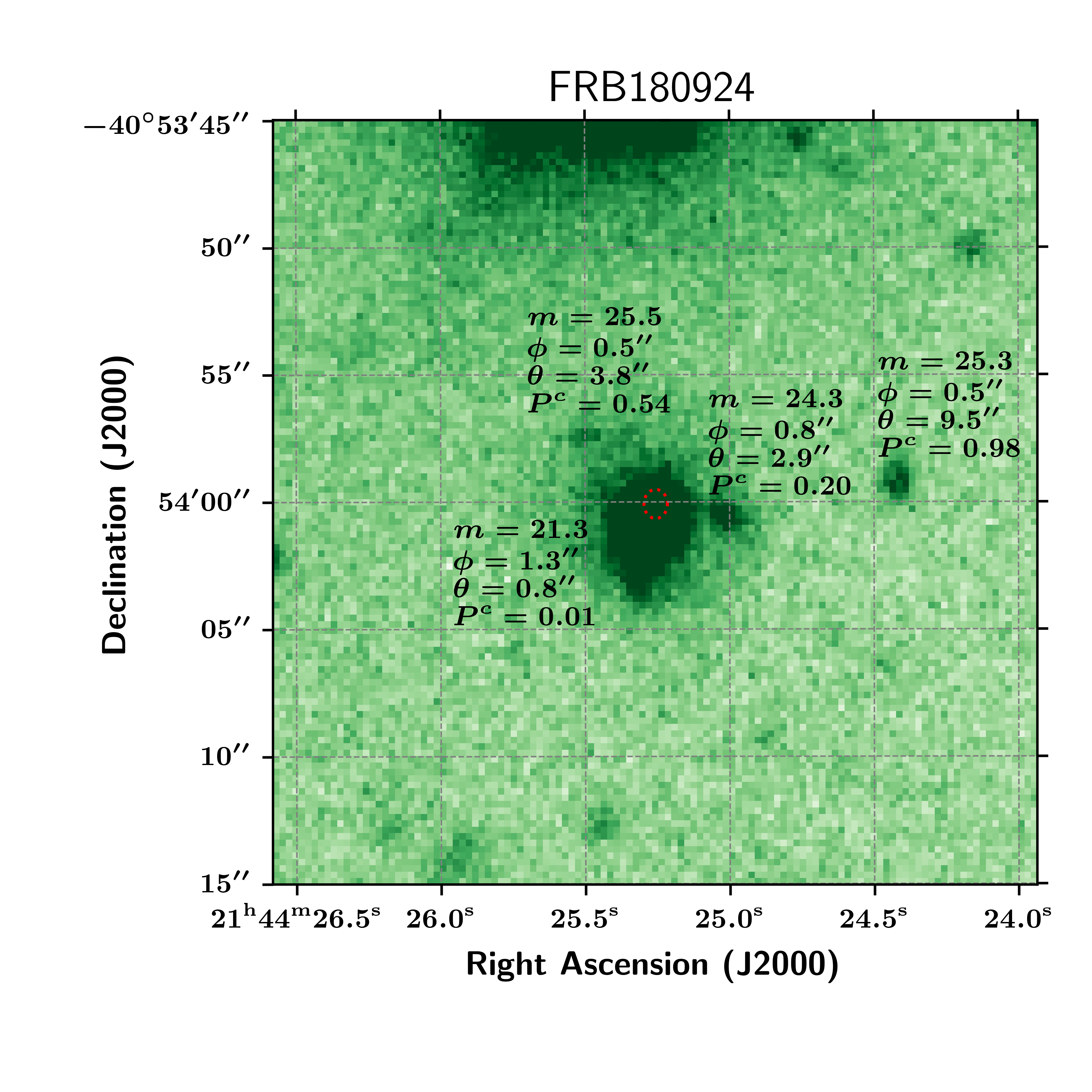
Figure 1: Cutout $g$-band image (VLT/FORS2) centered on FRB 180924 (small red circle indicates the $5\sigma$ localization). There are four extended sources with separation $\theta<10^{\prime\prime}$ marked as candidates for the host galaxy of the FRB. These are labeled (just above them, except for the brightest) by their $\theta$, angular size $\phi$, apparent magnitude $m$, and the chance probability $P^{c}$ of an association.

2 Historical: Chance Probability

A standard approach to associating transients to their host galaxies is through assessing the chance probabilities $P^{c}$ of galaxies being located close to the transient position. We reintroduce the formalism for evaluating $P^{c}$ here, propose a new variant, and comment further on its application and limitations.

2.1 Formalism

Figure 1 shows a VLT/FORS2 $g$-band cutout image ($30^{\prime\prime}\times 30^{\prime\prime}$) of the field surrounding FRB 180924 with its localization marked by a red circle. As described by Bannister et al. (2019), this localization lies $\approx 1^{\prime\prime}$ from the centroid of galaxy DES J214425.25$-$405400.81 and within $5^{\prime\prime}$ of two additional galaxies. At their redshifts (Bannister et al., 2019), the galaxies all have projected separations of less than 40 kpc, i.e. separations less than the estimated radii of their halos. Therefore, while one may be predisposed to assign FRB 180924 to the brighter and closer galaxy, one should also entertain the possibility that the FRB occurred in the stellar halo of one of the others.

The chance probability approach is powerfully simple: estimate the Poisson probability of finding one or more galaxies as bright or brighter within an effective search area $A$ around the FRB, with $A$ determined from the angular size $\phi$, the separation $\theta$, and the FRB localization uncertainty $\sigma_{\rm FRB}$. Namely, one defines the probability of a chance coincidence

$$P^{c}(\theta_{\rm eff},m)=1-\exp(-\bar{N})\;\;\;,$$ (1)

where $\bar{N}$ is the average number of sources in $A$. It is given by

$$\bar{N}(\theta_{\rm eff},m_{i})=\pi\theta_{\rm eff}^{2}\,\Sigma(m_{i})\;\;\;,$$ (2)

where $\Sigma(m)$ is the angular surface density of galaxies on the sky with magnitude $m\leq m_{i}$, and $\theta_{\rm eff}$ is the effective search radius ($A=\pi\theta_{\rm eff}^{2}$). For the former, we adopt the galaxy number count distribution of Driver et al. (2016), while the latter quantity bears some arbitrariness.

Previous works have considered several definitions for $\theta_{\rm eff}$. We introduce yet another more conservative one here: the quadrature sum of all three angular quantities with semi-arbitrary weightings,

$$\theta_{\rm eff}=\sqrt{4\sigma_{\rm FRB}^{2}+\theta^{2}+4\phi^{2}}\;\;.$$ (3)

Adopting these, we estimate $P^{c}=0.01$ for DES J214425.25$-$405400.81 and $P^{c}>0.1$ for the other sources owing to their fainter magnitudes and larger angular separations. From this perspective, the probability of a chance association is nearly negligible for DES J214425.25$-$405400.81 and sufficiently large for the other sources that one is inclined to favor the former. However, this technique cannot assign a likelihood to this association, nor even a relative assessment of one source over another. Yet worse, if two or more candidates have low $P^{c}$ (e.g. FRB 181112; Prochaska et al., 2019), one has no means to favor one over the other. Last, the $P^{c}$ formalism does not naturally allow one to introduce additional observational measures as evidence (e.g. DM). Together, these considerations motivate our development of a full probabilistic treatment.

2.2 Nuisances and Nuances

There are several aspects of the $P^{c}$ analysis that require further definition. For completeness, we describe these here although $P^{c}$ does not formally enter into the new formalism. First, one requires measurements of the galaxy centroids and angular size. We advocate a non-parametric approach owing to the complexity of galaxy morphology. In the following, we adopt the centroiding algorithm encoded in the photutils software package, and use the semimajor_axis_sigma parameter to estimate the angular size. In the following, we will refer it as a_image as it matches the definition of that parameter in the more widely used sextractor package.

Another issue is Galactic extinction. FRBs are detected across the sky including on sightlines that show large Galactic extinction ($E(B-V)>0.1$ mag). In contrast, the number count analyses have intentionally been derived from high-latitude fields with low Galactic extinction. Therefore, the apparent magnitudes of the galaxy candidates should be corrected for Galactic extinction prior to the probability estimation.

We provide the following set of recommendations to optimize the detection and characterization of both faint and bright sources. Namely, we recommend observations in the $r$-band, which provide a trade-off between the mapping of stellar content and extinction. We further recommend an image depth of $m_{r}=25.5$ ($5\sigma$), corresponding to the limiting magnitude for spectroscopy, and sufficient for probing $0.01\ L^{*}$ galaxies at $z\sim 0.5$. Finally, given the subarcsecond accuracy of many FRB localizations, we recommend better than $1^{\prime\prime}$ seeing, and a $>1^{\prime}$ field of view for background estimation.

Similarly, source detection should employ a non-parametric approach to accommodate galaxies of varying morphologies. For consistency with this work, we recommend use of the a_image parameter to estimate the angular size of sources, and note that all galaxies should be corrected for Galactic extinction prior to applying the Bayesian formalism.

The formalism of eq.(1) and (2) ignores galaxy clustering. Since matter in the Universe is not uniformly distributed, the probability of observing either no galaxies, or a large number of them, in proximity to a random direction is enhanced compared to the probability of observing one or a few. Tunnicliffe et al. (2014) show that including clustering decreases the probability of a nearby random galaxy by 25–50% in the case of a random direction. Our primary concern however is not whether or not all the observed galaxies are merely chance coincidences, but rather which of the observed galaxies is the true host. Clustering is discussed further in this context in section 4.2. For now, we remark that given that FRBs truly are associated with galaxies, clustering acts to increase, not decrease, the probability of a chance association, since the FRB observation has preferentially selected a direction of the Universe in which there is a cluster of matter.

Furthermore, in this work we ignore for the sake of simplicity the ellipticity of the prospective host galaxies. Our method will be readily adaptable however to such ellipticity, or indeed arbitrarily complex functions, since the approach described below does not rely on any particular functional forms.

3 Probabilistic Approach

Association of transients to galaxies is not like the usual cross-identification for which probabilistic methods have been in place for over a decade (Budavári & Szalay, 2008). Matching stars and galaxies typically involves asking whether a set of detections (across separate exposures, instruments, telescopes) are of the same celestial object. If they are, their true (latent) directions would have to be the same; see more in the review by Budavári & Loredo (2015).

In strong contrast with that, FRBs are presumed to simply originate from within (or at least near to) galaxies, hence their true direction should not be required to coincide with the center of a galaxy. While this is admittedly a small difference for the faintest galaxies, resolved extragalactic source are expected to yield different results. Here we consider a general scenario where the shape of galaxies can be incorporated along with a geometric model about from where FRBs would originate within or around galaxies.

3.1 General Formalism

Since FRBs are sparse on the sky, we can study them separately, which also simplifies the following description of our approach. Let us consider a catalog of galaxies across the entire sky and a single FRB that either belongs to one of the many catalog objects (its host galaxy) or it does not, i.e. its host is not detected or not included in the catalog. If $U$ is the event that the FRB’s host is unseen, and $O_{i}$ is the event that the FRB is from galaxy $i$, their prior probabilities must add up to one,

$$P(U)+\sum\limits_{i}P(O_{i})=1\;\;\;,$$ (4)

as there are no other possibilities. The single scalar quantity $P(U)$ encodes all the complications that arise from the difference in the radial selection functions of the catalog and the FRB instruments. For now, we assume its value to be known, but note that it could be inferred in a hierarchical fashion when considering multiple FRBs. Also, one could assume a uniform prior for all observable $O_{i}$ as the simplest possible scenario that essentially ignores any additional information about the galaxies, e.g., magnitude, color, redshift. We leave such considerations to a future work.

Given a vector $x$ representing all measured properties of the detected FRB, we ask what the posterior probabilities $P(U|x)$ and $P(O_{i}|x)$ are for all $i$. Using Bayes’ rule, the unseen posterior is

$$P(U|x)=\frac{P(U)\,p(x|U)}{p(x)}\;\;\;,$$ (5)

where $p(x|U)$ is the probability density of the FRB properties given the host is unseen. From hereon, we consider $x$ to represent only the measured FRB direction. Without constraints, $x$ could be anywhere on the sky, hence it is natural to assume a uniform (isotropic) distribution with a value of $1\big{/}4\pi$. Similarly, the posterior probability for object $i$ is

$$P(O_{i}|x)=\frac{P(O_{i})\,p(x|O_{i})}{p(x)}\;\;\;,$$ (6)

where $p(x|O_{i})$ is the probability density function (PDF) of $x$ given that the FRB comes from galaxy $i$. With data $x$, this is the marginal likelihood of $O_{i}$, which includes the galaxy geometry and the uncertainty of the FRB direction. This key component of the approach is discussed in depth in the next paragraph. The normalizing constant must be

$$p(x)=P(U)\,p(x|U)+\sum\limits_{i}P(O_{i})\,p(x|O_{i})\;\;$$ (7)

to guarantee that these posteriors also add up to one,

$$P(U|x)+\sum\limits_{i}P(O_{i}|x)=1\;\;.$$ (8)

3.2 Marginal Likelihoods

Let the 3-D unit vector $\omega$ represent the true and unknown direction of the FRB on the sky. Given that it comes from a particular galaxy, the direction $\omega$ has to point somewhere near the host. The function $p(\omega|O_{i})$ captures the physical and geometric model for the FRBs specific to galaxy $i$, e.g., taking into account its type, distance, orientation, etc.

The observed FRB direction $x$ is a measurement of $\omega$ with known uncertainty, represented by the localization error function, $L(x-\omega)$. Given $p(\omega|O_{i})$, $p(x|O_{i})$ is calculated by integrating over the $\omega$ model directions to obtain the marginalized likelihood of the association hypothesis $O_{i}$,

$$p(x|O_{i})=\int\!\!d\omega\,p(\omega|O_{i})\,L(x-\omega)\ ,$$ (9)

which now accounts for all possibilities in various FRB origins as well as the astrometric uncertainty in the measurement. If a galaxy is unresolved, $p(\omega|O_{i})$ may become the Dirac-$\delta$, and $p(x|O_{i})$ is just the astrometric uncertainty, as it would be the case for matching point sources. Calculating the above quantity for all $i$ completes the framework, which now provides posterior probabilities via eq. 6.

3.3 Limited Field of View

Previously we assumed a galaxy catalog over the entire sky, but catalogs typically have more limited footprints. It is interesting to think about a scenario when the field of view $\Omega$ is smaller but still large enough not to miss any possible counterparts to the FRB in question. Intuitively, galaxies very far away from the FRB should not have any effect on the association analysis.

Smaller sky coverage would mean fewer observed galaxies $N_{c}$, which in turn affect the $P(O_{i})$ priors as there are fewer galaxies to choose from. Going with the previous uniform assumption, eq.(4) implies

$$P(O_{i})=\frac{1-P(U)}{N_{c}}\;\;,$$ (10)

which captures the dependence.

Looking now back at Bayes’ rule in eq.(5), the sky coverage seems to affect the $P(O_{i}|x)$ posteriors, too. Fortunately, this is not the case. The denominator $p(x)$ changes in accord due to the scaling in $p(x|U)$, which is uniform over the field of view,

$$p(x|U)=\frac{\boldmath{1}_{\Omega}(x)}{\Omega}$$ (11)

where the $\boldmath{1}_{\Omega}(x)$ is the indicator function that takes the value 1 if $x$ is within the field of view and 0 otherwise, and the denominator $\Omega$ normalizes the PDF. The framework not only matches common-sense expectations, but provides for more efficient computation where only candidates within close proximity of FRBs are considered.

Given the plethora of deep, wide-field imaging surveys, it is possible to consider very large $\Omega$ for each FRB in the analysis. In practice, however, sensible and conservative assumptions for $p(\omega|O_{i})$ will greatly limit the list of viable candidates $O_{i}$. To ease the analysis, we adopt for $\Omega$ the union of the area encompassing all galaxies within 10 half-light radii and the 99.9% FRB localization. As emphasized in the previous section, it is only necessary to consider a large enough area to be certain to include all possible hosts.

4 Priors and Assumptions

4.1 Undetected Prior $P(U)$

It is difficult to a priori assign a prior $P(U)$ to the probability that the FRB host is undetected. Undoubtedly, $P(U)$ is related to the depth of the imaging and the (unknown) source distance, i.e. redshift. In the following, we consider an arbitrarily assigned value, and we advocate a low value, based on the paucity of our data and the set of confidently assigned associations reported to date (e.g. Heintz et al., 2020). In the analyses that follow, we typically assume $P(U)=0$ (Occam’s razor!) and discuss the impacts of increasing it.

4.2 Candidate priors $P(O)$

For the set of host candidates $O_{i}$, absent any assumptions on the distance or the typical separations of FRBs from their host galaxies, any galaxy on the sky could be a viable candidate. Given the plethora of potential models for FRB progenitors and the limited existing constraints, we are motivated to consider (for now) simple approaches to the prior for the galaxy candidates. The most agnostic approach is to assign an “identical” prior to every galaxy in consideration, i.e. eq. 10.

Inspired by the chance probability calculations approach described in $\S$ 2, we introduce an additional prior based on $P^{c}$. Specifically, we consider a prior that inversely weights by $\Sigma(m)$.

$$P(O_{i})\propto\frac{1}{\Sigma(m_{i})}\;\;.$$ (12)

For this “inverse” prior, brighter candidates have higher prior probability according to their number density on the sky. The normalization of these priors is set by eq. 4. In section 5 we also briefly consider two other priors with $P(O_{i})\sim 1/\Sigma(m_{i})\phi$ (inverse1) and $P(O_{i})\sim 1/\Sigma(m_{i})\phi^{2}$ (inverse2). We adopt the prior in Equation 12 in part because of its simpler form and also because of the results of simulated experiments (Section 5).

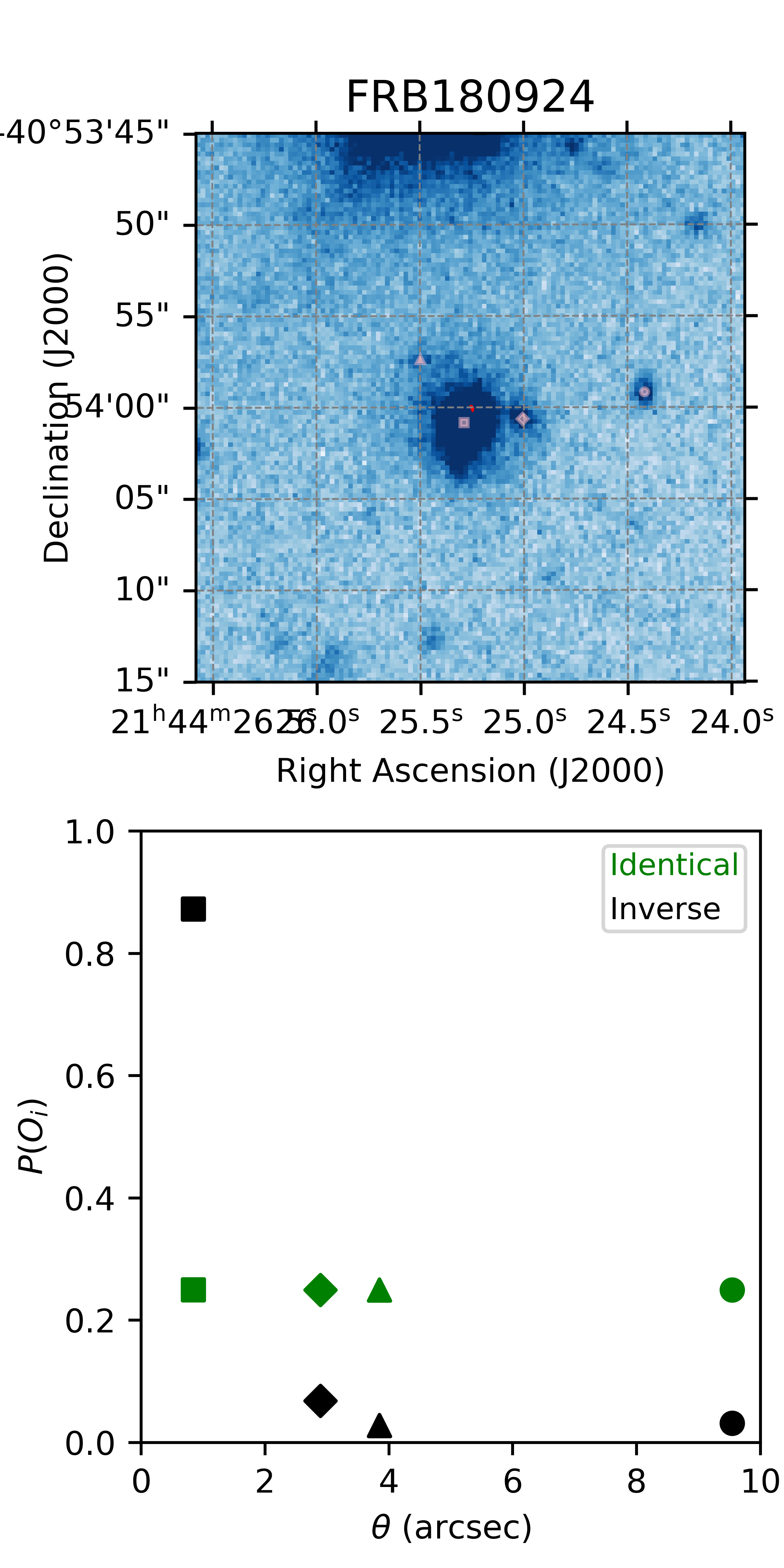
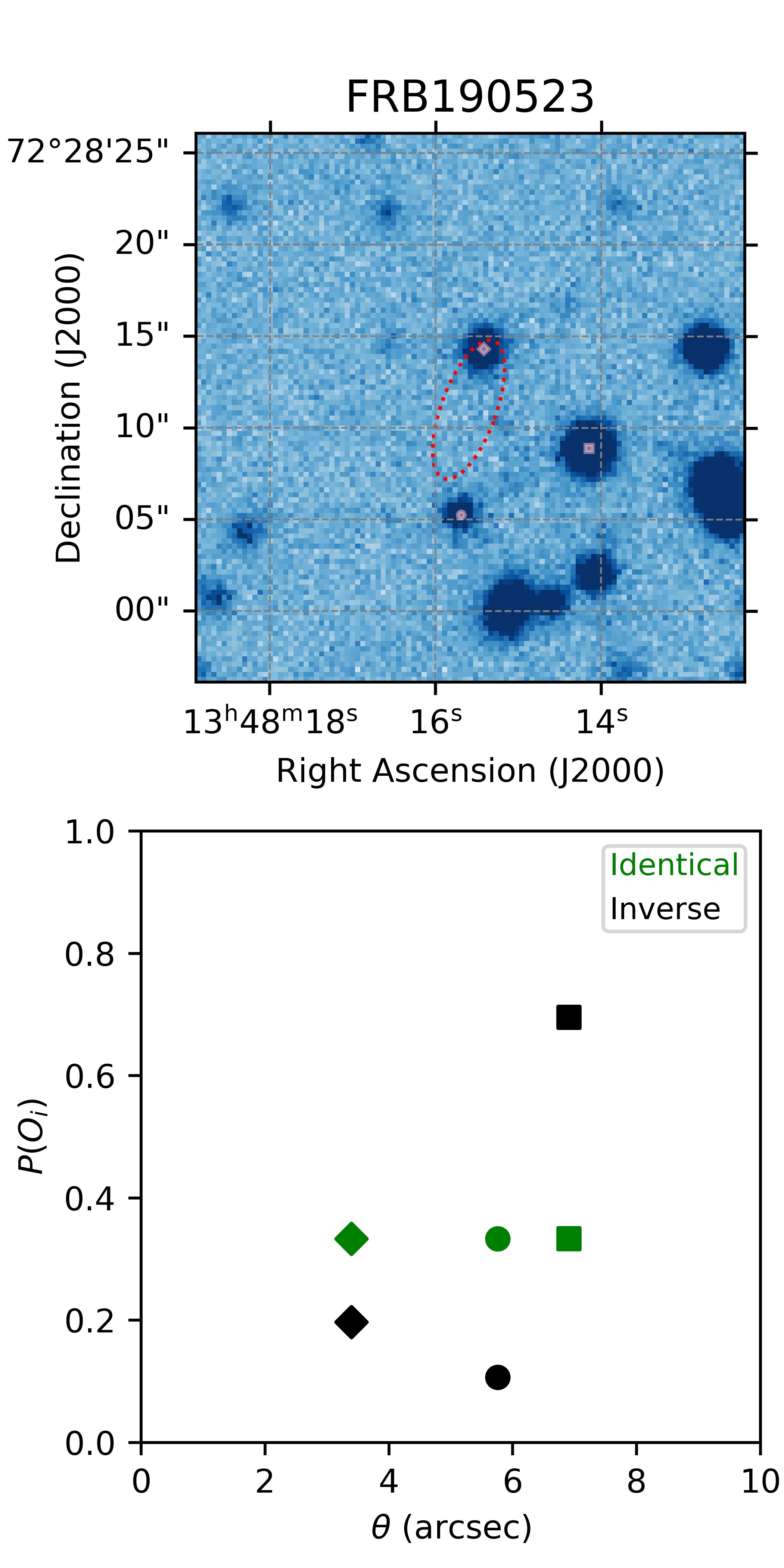
Figure 2: Illustration of the two approaches to candidate priors $P(O)$ assumed in this manuscript: identical and inverse. The former assumes an identical prior for every galaxy with $\theta_{i}<10\phi$ or within the 99.9% localization error of the FRB. The latter adopts the inverse of the estimated chance probability $P^{c}$ of these galaxies which is equivalent to asserting the prior is proportional to the integrated probability that the other sources are all chance coincidences.

Figure 2 illustrates $P(O_{i})$ for the two models for two example cases – (a) FRB 180924 and (b) FRB 190523 – where we assume $P(U)=0$. For this illustration, we have restricted the analysis to galaxies within $10^{\prime\prime}$ of the FRB, which captures all of the viable candidates. As expected, the inverse priors for FRB 180924 significantly favor the brighter galaxy closest to the FRB. Perhaps less intuitively, the inverse priors favor the most distant (yet brightest) source near FRB 190523. This motivates the inclusion of the next ingredient — the offset function $p(\omega|O_{i})$.

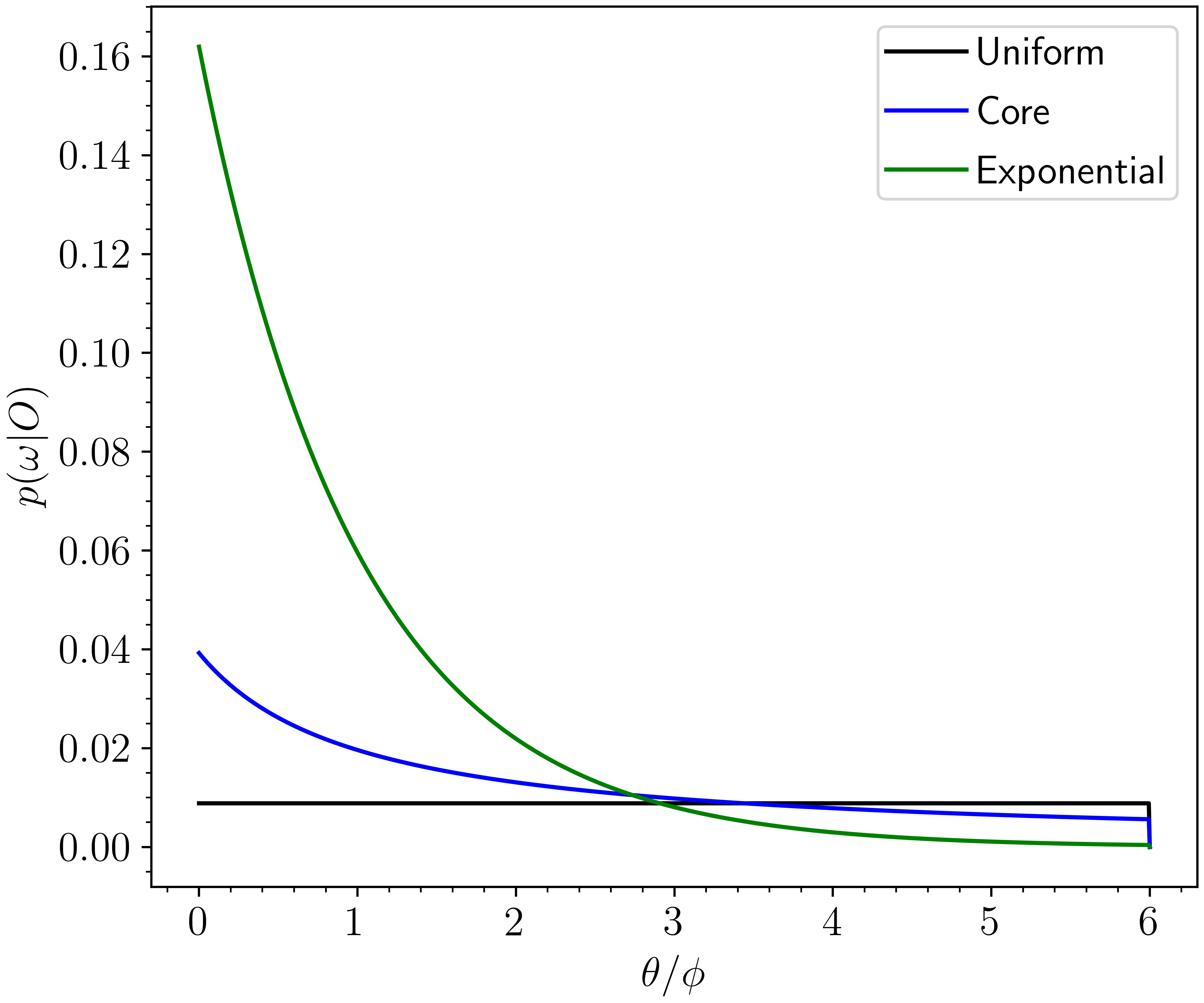
Figure 3: Three offset functions $p(\omega|O_{i})$ considered for the underlying angular distribution of FRBs relative to their host galaxies, normalized by the galaxy’s half-light radius $\phi$. Each is normalized to have identical integrated area to a maximum assumed offset of $\theta_{\rm max}=6\,\phi$.

4.3 Offset function $p(\omega|O_{i})$

The $p(\omega|O_{i})$ function for the probability of the true angular offset from the galaxy is unknown yet required for the analysis. In our formalism, we develop priors for $p(\omega|O_{i})$ based solely on the angular offset $\theta$ between the galaxy centroid and $\omega$, and also normalized by the observed galaxy’s angular size $\phi$. This simultaneously accounts for galaxies of different intrinsic size and differing observed size owing to their distance.

As the predominance of models associate FRBs to stellar sources or compact objects (AGN at the very centers of galaxies are currently disfavored; Bhandari et al., 2020a), one might expect the FRB events to track the stellar light. While we wish to remain largely agnostic to the underlying distribution of offsets, we are physically motivated to presume $p(\omega|O_{i})$ decreases with increasing $\theta$. We assert this despite the fact that geometrical considerations do favor large $\omega$, e.g. a model where FRBs occur with identical probability anywhere in a circular galaxy will have $p(\omega|O_{i})\propto\omega$ until one reaches the “edge” of the galaxy. Therefore, a uniform prior $p(\omega|O_{i})=1/\pi\theta_{\rm max}^{2}$ is formally one that assumes FRBs occur proportional to the galaxy radius. The other two models considered are a core model:

$$p(\omega|O_{i})=\frac{1}{2\pi\phi^{2}[\theta_{\rm max}/\phi-\log(\theta_{\rm max}/\phi+1)]}\frac{1}{(\theta/\phi)+1}\;\;\;,$$ (13)

which implies an approximately $1/r^{2}$ weighting, and an exponential model

$$p(\omega|O_{i})=\frac{1}{2\pi\phi^{2}[1-(1+\theta_{\rm max}/\phi)\exp(-\theta_{\rm max}/\phi)]}\exp[-\theta/\phi]\;\;\;,$$ (14)

which assumes an underlying exponential distribution. All of these functions are normalized to unity when integrating to $\theta_{\rm max}$, ignoring the curvature of the sky.

For all of the $p(\omega|O_{i})$ priors, we assert a maximum offset $\theta_{\rm max}=6\phi$; this is especially important for the uniform prior. This value is arbitrary and was chosen to be large enough to accommodate prevailing models of FRBs without being too conservative.

Applying an arbitrary cutoff to the exponential distribution is not strictly necessary, but we keep it for simplicity and consistency, and demonstrate in Section 6.3 that the results for an exponential distribution are insensitive to this choice.

Figure 3 shows the offset functions, normalized to have the same total probability. Clearly the exponential model favors FRBs located in the inner regions of galaxies. For comparison to the offset distributions of known transients, we note that long GRBs appear highly concentrated in the inner regions of their hosts relative to Type Ib/c and IIn supernovae, which occur preferentially near their host half-light radii (Lunnan et al., 2015; Blanchard et al., 2016). Conversely, short GRBs exhibit significant offsets from their host centers, indicative of progenitors born in compact object mergers (Fong & Berger, 2013).

In practice, we treat the galaxies as “round”, i.e. ignoring for now any ellipticity. Future works will advance this aspect.

5 Simulations

To explore the formalism introduced here, we have generated Monte Carlo simulations designed to faithfully reproduce the FRB experiment. We describe this first and then detail the results.

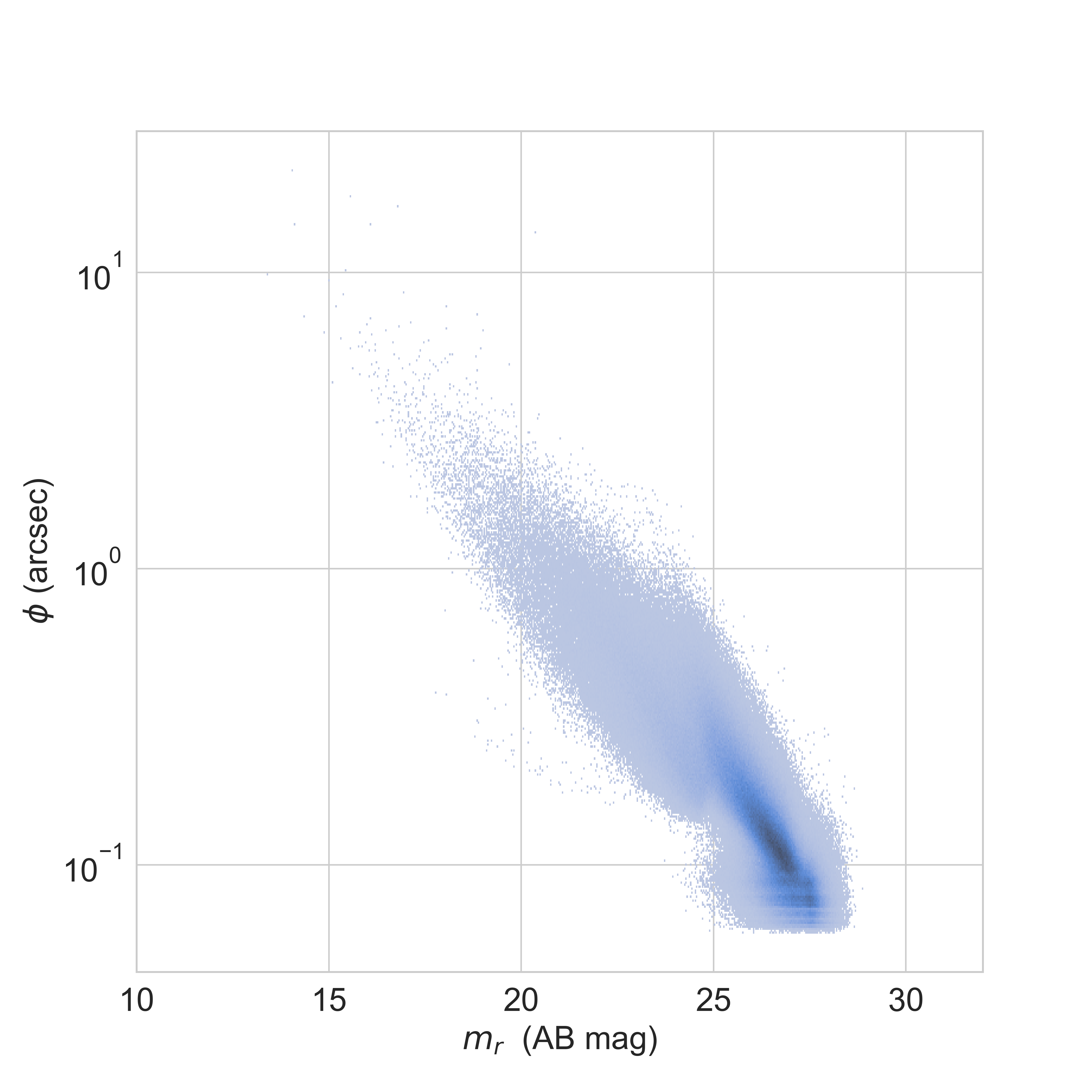
Figure 4: Distribution of angular sizes (a_image parameter) versus apparent magnitude $m_{r}$ for all of the galaxies in the COSMOS catalog (Scoville et al., 2007a).

5.1 Sandboxes

Our Monte Carlo approach leverages the public catalog of the HST/COSMOS field (Scoville et al., 2007b, a) which provides over 1 million sources at high spatial resolution and faint fluxes (median AB magnitude $m_{r}\approx 25.9$). These galaxies are distributed over an $\approx 1$ sq. deg of sky which captures a great variety of distributions but not the most extreme events (e.g. $z<0.5$ galaxy clusters, nearby galaxies). Figure 4 shows the angular size (a_image) and apparent magnitudes for the catalog, restricted to the sources labeled as galaxies.

We generate a series Monte Carlo realizations of FRBs (referred to as a sandboxes, or SBs), using the following recipe:

1. Define the true distribution of FRBs from their host galaxies $p(\omega|O_{i})$and magnitude $m_{r}$.

2. Define a sample of potential host galaxies based on $m_{r}$.

3. Define the distribution of localization errors for FRBs ($\sigma_{\rm FRB}$).

4. Draw $N_{\rm FRB}$ galaxies from the parent sample of potential host galaxies without duplicates.

5. Set the true FRB positions according to $p(\omega|O_{i})$.

6. Offset the FRBs to an observed coordinate according to $\sigma_{\rm FRB}$.

7. Consider catalogue galaxies within $30^{\prime\prime}$ to represent an image.

For sandbox 5 (SB-5), 10% of the FRBs were randomly placed in the COSMOS field, i.e without a host galaxy. We plan to use this sandbox to evaluate the performance of the framework when the host galaxies are unseen. Also, as COSMOS is a deep survey, we generate a magnitude-limited catalog of galaxies for each sandbox (last column of Table 1) on which we run the Bayesian framework. In the following sub-section, we discuss results for five sandboxes (focusing primarily on SB-1) with the parameters described in Table 1.

Table 1: SandBoxes

Label	$p(\omega|O_{i})$	$N_{\rm FRB}$	Sample	$\sigma_{\rm FRB}$	Catalog Filter
				(′′)
SB-1	$\mathcal{U}(0,2\phi)$	100,000	-	1	-
SB-2	$\mathcal{U}(0,2\phi)$	46,699	$m_{r}=[20,23]$	$\mathcal{U}(0.1,1)$	$m_{r}\leq 23$
SB-3	core	46,699	$m_{r}=[20,23]$	$\mathcal{U}(0.1,1)$	$m_{r}\leq 23$
SB-4	exponential	46,699	$m_{r}=[20,23]$	$\mathcal{U}(0.1,1)$	$m_{r}\leq 23$
SB-5	$\mathcal{U}(0,2\phi)$	50,000	$m_{r}=[20,25]$	$\mathcal{U}(0.1,1)$	$m_{r}\leq 25$

Table 2: Sandbox Analysis

Sandbox	$P(O)$	$P(U)$	$p(\omega|O_{i})$	$\theta_{\rm max}$/$\phi$	f(T+secure)	TP
SB-1	inverse	0	exp	6	0.33	0.96
SB-1	inverse1	0	exp	6	0.30	0.99
SB-1	inverse2	0	exp	6	0.32	1.00
SB-1	identical	0	uniform	6	0.22	1.00
SB-1	inverse	0.05	exp	6	0.24	0.96
SB-2	inverse	0	uniform	2	0.86	1.00
SB-3	inverse	0	core	6	0.58	1.00
SB-4	inverse	0	exp	6	0.68	0.99
SB-5	inverse	0.10	exp	6	0.58	0.98

5.2 Analysis and Results

We now analyze the sandboxes listed in Table 1 with a variety of priors and assumed $p(\omega|O_{i})$ functions (that generally do not match the true $p(\omega|O_{i})$). Table 2 lists the various priors assumed for each analysis performed.

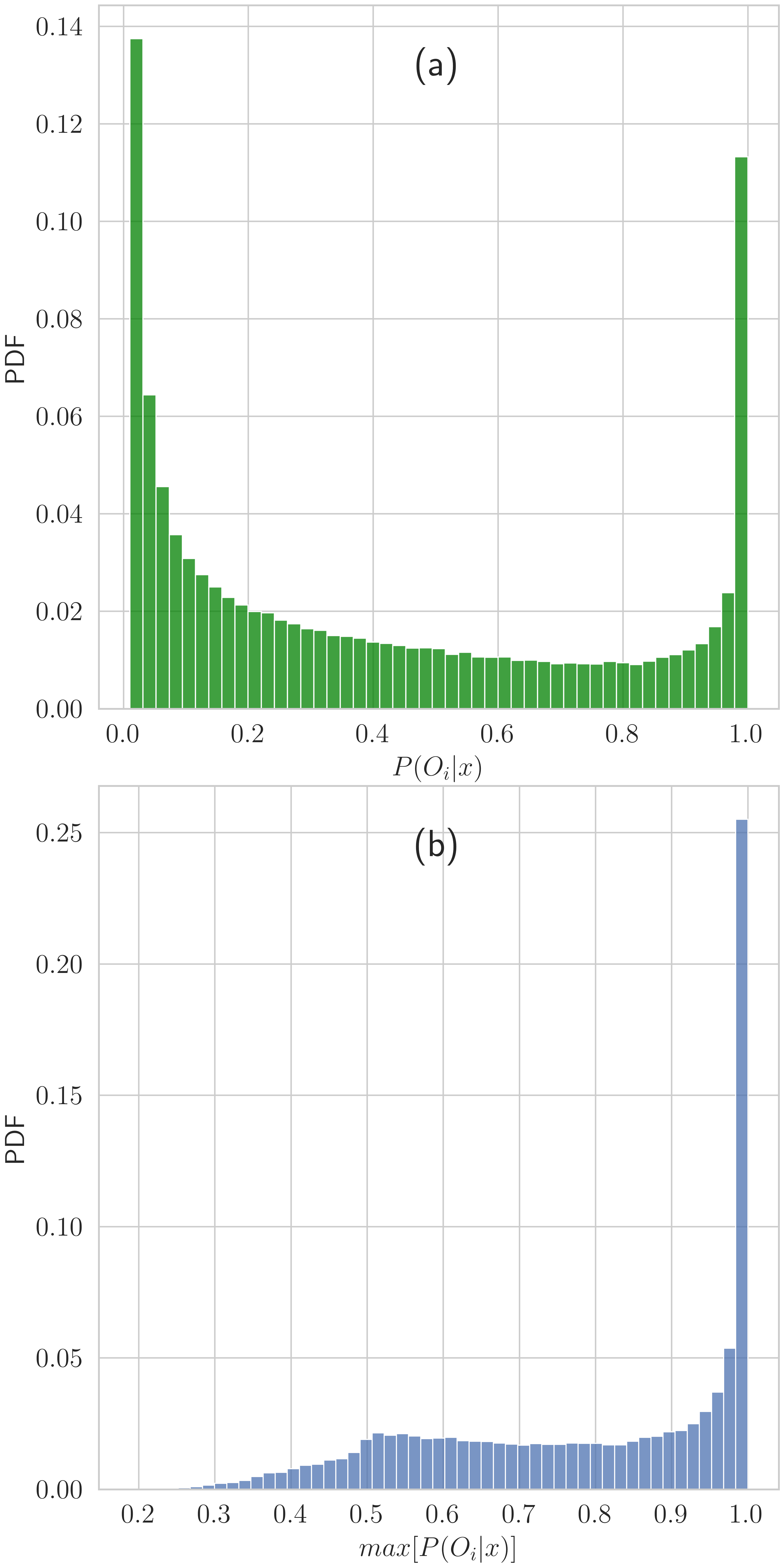
Figure 5: Analysis of SB-1: (a) PDF for the posterior probabilities for all of the candidates with $P(O_{i}|x)>0.01$. The PDF is nicely bi-modal with 96% having $P(O_{i}|x)<10\%$ or $P(O_{i}|x)>90\%$. (b) PDF of the maximum posterior for the 100,000 simulated FRBs. We find $\approx 35\%$ of the sources has $P(O_{i}|x)>0.95$, which we define as secure.

Figure 5a shows the posteriors for the candidates using the fiducial sandbox (SB-1) and listed in row 1 of Table 2 (also referred to as the adopted prior set; Table 3). Since most of the candidates defined in step 7 are very far from the offset FRB position, we restrict results to the $\approx 8\%$ of candidates with $P(O_{i}|x)>0.01$. This distribution is multi-modal, with the overwhelming majority of recovered $P(O_{i}|x)\approx 0$ corresponding to unassociated galaxies and another peak at $P(O_{i}|x)\approx 1$ corresponding to secure associations. Figure 5b shows the posterior value for the most probable candidate for each of the 100,000 FRBs. For this model and analysis, $\approx 35\%$ of the FRBs have a high probability, $P(O_{i}|x)>0.95$ which we adopt as a “secure” association. Adopting such an arbitrary value to define ‘secure’ is useful for including/excluding candidates for subsequent analyses that rely on knowing the correct FRB host, e.g. that by Macquart et al. (2020). However, we emphasise that it is in-general better to consider all host associations as uncertain, with different levels of certainty according to the obtained posteriors.

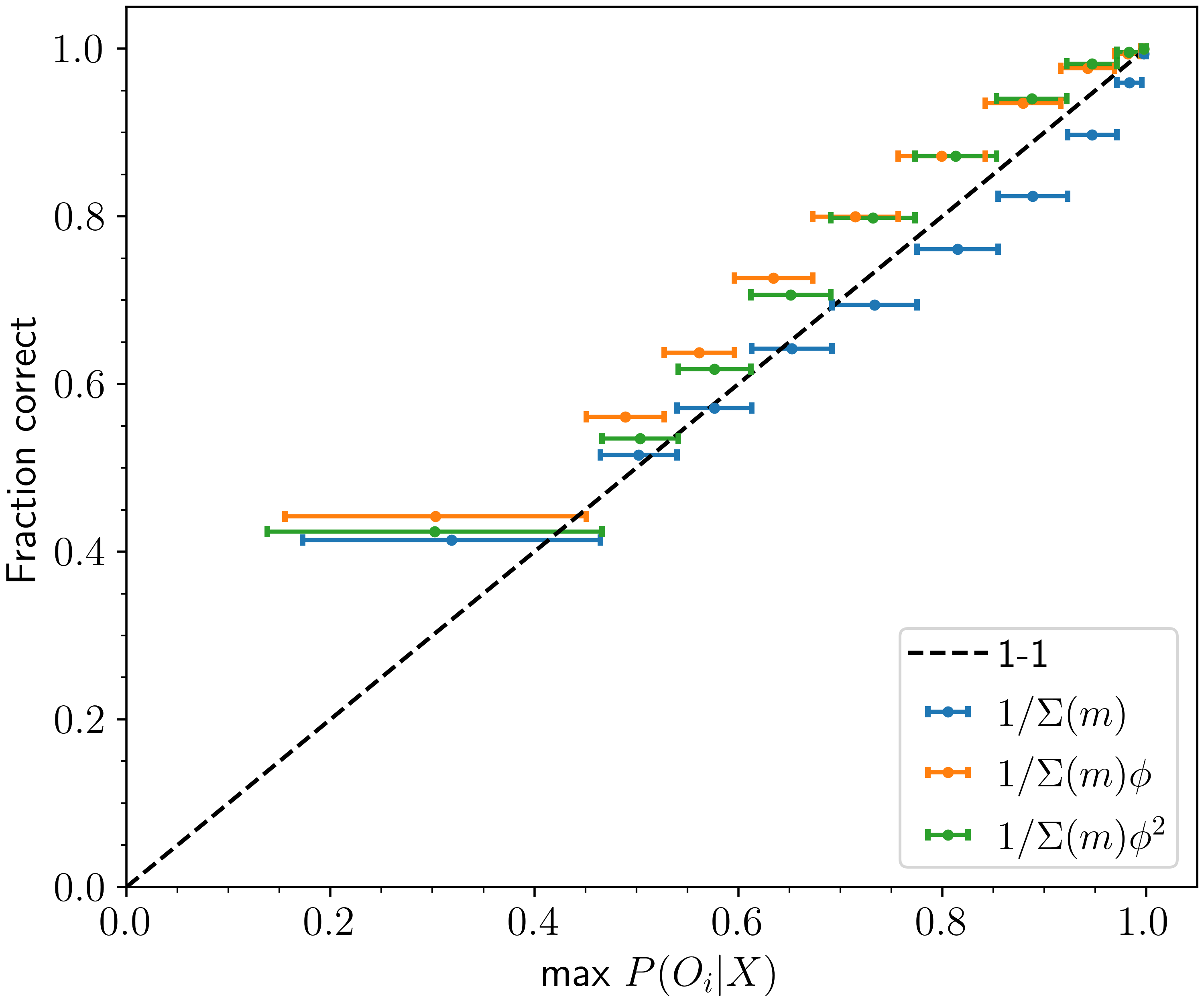
Figure 6: The points are equal number (10,000) bins of FRBs according to the maximum posterior probability of their host candidates for SB-1. For each set of 10,000 we determined the fraction of correct assignments if one adopts the candidate with max $P(O_{i}|x)$ as the host. The one-to-one line indicates a perfectly calibrated algorithm. The colors indicate different choices for the prior $P(O)$: (blue) $P(O)\propto 1/\Sigma(m)$, inverse; (orange) $P(O)\propto 1/\Sigma(m)\phi$, inverse1; (green) $P(O)\propto 1/\Sigma(m)\phi^{2}$, inverse2. Our adopted prior (inverse) is relatively well normalized in that $P(O_{i}|x)$ yields an accurate estimate of the fraction of FRBs correctly assigned to their host galaxy.

Figure 6 evaluates, in 10 bins of equal number of FRBs, the maximum $P(O_{i}|x)$ assigned to a candidate for each FRB and the percentage of correct associations assuming this is the host. The different colors indicate different choices for $P(O)$. Our adopted “inverse” prior appears well calibrated in that $P(O_{i}|x)$ yields an accurate estimate of the fraction of FRBs correctly assigned to their host galaxy.

Figure 8 shows another set of results but for more different choices of priors (Table 2). The remarkably close correspondence between the two quantities indicates the posterior is well-calibrated, at least for this pairing of sandbox and prior set. We also show results for prior sets where we assume $P(U)=0.05$ and for the conservative prior set (Table 3). Each of these assigns systematically lower values to the true host galaxy yielding a higher percentage of correct cases at lower maximum $P(O_{i}|x)$.

To characterise the behaviour of our method under different simulated truths (i.e., sandboxes) and different priors, Table 2 lists the fraction $f$ of all FRBs which are correctly identified, i.e. the true (T) host is securely identified ($P(O_{i}|x)>0.95$); and the fraction of secure identifications which are correct. In all cases, at least 96% of all secure associations find the true host, indicating that our method is trustworthy. The fraction of FRBs expected to have such a secure association however varies significantly, primarily as a function of the sandbox (variation of $\pm 0.3$ in $f(T+{\rm secure})$), with the analysis method on a given sandbox having a secondary effect (variation of $\pm 0.05$). Analysis of SB-1 demonstrates that the choice between different inverse priors has little effect, but produces a higher fraction of secure associations than a uniform prior. Interestingly, $f(T+{\rm secure})$ is much higher for the SB-4 analysis than for SB-2 and SB-3, despite all three using an assumed $p(\omega|O_{i})$ of equal shape to the true $p(\omega|O_{i})$, and being otherwise identical. However, while the SB-4 analysis assumes $p(\omega|O_{i})$ to be uniform out to $\theta=6\phi$, the true distribution is fully contained within $2\phi$, unlike SB-2 and SB-3. We thus conclude that the dominant determinant of the fraction of securely (and hence, correctly) identified FRB hosts, in the case that the true host is observed, is the fraction of FRBs lying in close proximity to their hosts, irrespective of other considerations. We find it especially reassuring that results are not highly sensitive to the analysis method, i.e. that our formalism yields greater sensitivity to the physical truth than to our choice of reasonable priors.

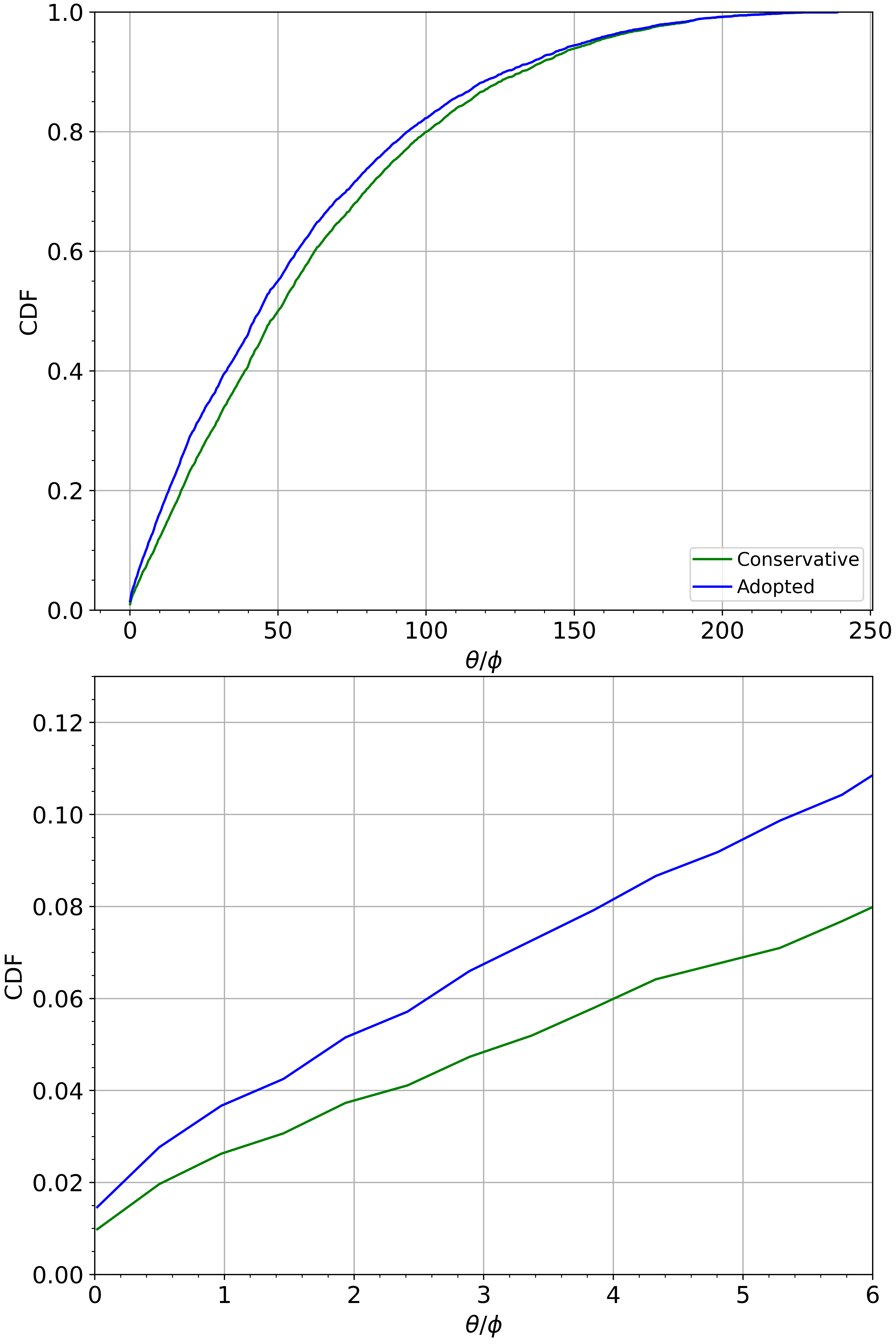
Figure 7: Cumulative distribution of $\theta/\phi$ for candidate galaxies in SB-5 where the true host is unseen, using conservative (green) and adopted (blue) priors. Lower panel is a zoom-in on the region related to our adopted maximum offset.

What about unseen hosts? If we use $P(U)=0$, as typically assumed in this work, then $P(U|x)=0$ always, and the method will tend to assign the highest posterior $P(O_{i}|x)$ to the closest galaxy regardless of distance. Using the 10% of hostless FRBs from SB-5, the conservative and adopted prior sets from Table 3 find secure associations for the majority of FRBs (55% and 62% respectively). However, the typical radial offset for these secure associations is very large. In Figure 7, we show the cumulative distribution of $\theta/\phi$ for such candidates. The probability of the most likely candidate being close to the FRB is small, with 10% or less of such falsely identified hosts having $\theta/\phi<6$. The distributions for secure associations is almost identical to that from non-secure hosts. We conclude that measuring a small $\theta/\phi$ is a strong discriminant against unseen hosts irrespective of $p(U)$.

Buoyed by these results, we now proceed to apply PATH to real FRB observations.

Figure 8: Same as Figure 6 but for different prior assumptions as described in the legend.

Table 3: Prior Sets

Set	$P(O)$	$P(U)$	$p(\omega|O_{i})$	$\theta_{\rm max}$/$\phi$
Conservative	identical	0	uniform	6
Adopted	inverse	0	exp	6

6 Real FRB Analysis and Results

Informed by the results of the previous section, we proceed to apply the formalism to all of the published, well-localized FRBs. We discuss results for two sets of priors — conservative and adopted  — as summarized in Table 3. We refer to the first as conservative because all galaxies within $\theta_{\rm max}$ are given equal prior.

Table 4: FRBs Analyzed

FRB	$\alpha_{\rm FRB}$	$\delta_{\rm FRB}$	$\epsilon_{a}$	$\epsilon_{b}$	$\epsilon_{\rm PA}$	Filter
	(deg)	(deg)	(′′)	(′′)	(deg)
FRB121102	82.99458	33.14792	0.10	0.10	0.0	GMOS_N_i
FRB180916	29.50313	65.71675	0.00	0.00	0.0	GMOS_N_r
FRB180924	326.10523	-40.90003	0.11	0.09	0.0	VLT_FORS2_g
FRB181112	327.34846	-52.97093	3.25	0.81	120.2	VLT_FORS2_I
FRB190102	322.41567	-79.47569	0.54	0.47	0.0	VLT_FORS2_I
FRB190523	207.06500	72.46972	4.00	1.50	340.0	LRIS_R
FRB190608	334.01987	-7.89825	0.26	0.25	90.0	VLT_FORS2_I
FRB190611	320.74546	-79.39758	0.67	0.67	0.0	GMOS_S_i
FRB190614	65.07552	73.70674	0.80	0.40	67.0	LRIS_I
FRB190711	329.41950	-80.35800	0.40	0.31	90.0	GMOS_S_i
FRB190714	183.97967	-13.02103	0.36	0.22	90.0	VLT_FORS2_I
FRB191001	323.35155	-54.74774	0.17	0.13	90.0	VLT_FORS2_I
FRB200430	229.70642	12.37689	1.07	0.30	0.0	LRIS_I

Note. — $\epsilon_{a}$, $\epsilon_{b}$, $\epsilon_{\rm PA}$ define the total $1\sigma$ error ellipse for the FRB localization Data are taken from Ravi et al. (2019); Day et al. (2020); Law et al. (2020); Tendulkar et al. (2017); Marcote et al. (2020); Heintz et al. (2020).

6.1 FRB Host Candidates

Central to the analysis is the identification and analysis of galaxy candidates in imaging data. The first step — source identification — is the most challenging and the most subjective. For every image, sources near the detection limit are subject to the precise methodology: background subtraction, thresholding, pixel grouping, and deblending. After experimenting with the routines encoded in the photutils package, we settled on the following key parameters: npixels $=9$, deblend$=$True, xy_kernel $=(3,3)$, Gaussian2Dkernel, nsig $=3.$ (kernel), nsig $=1.5$ (threshold), background $=(50,50)$, filter_size $=(3,3)$, median background.

To test these choices, we independently analyzed the data with the SExtractor package using a standard set of input parameters. Namely, we set DETECT_MINAREA $=9$ and DETECT_THRES $=1.5$ for consistency with the photutils parameters. Images are filtered with the default convolution kernel (default.conv). To recover blended sources (see e.g., FRB 180924 below), we set DEBLEND_MINCONT $=0.0001$.

With this set of parameters, we recover the centroid positions within $\approx 2\%$, while the aperture sizes show scatter up to $\approx 15\%$. We note that slight differences between the photutils and SExtractor methodologies may be driving these discrepancies; namely, while SExtractor uses a multi-thresholding deblending technique, photutils utilizes a combination of multi-thresholding and watershed segmentation. Furthermore, the default.conv convolution kernel is equivalent to a $3\times 3$ Gaussian kernel with FWHM $=2$, in slight contrast to the Gaussian kernel used above. Nevertheless, we find comparable results using the two methods.

Figure 9: Segmentation images for the sources in $30^{\prime\prime}$ cutouts around FRB 180924 (left) and FRB 190523 (right). The multitude of sources (several erroneous) at the top of the FRB180924 image is due to artefacts from a very bright star.

Figure 9 shows the segmentation maps of FRB 180924 and FRB 190523. Note the three, blended sources near the localization of FRB 180924 which are known to be unique galaxies at distinct redshifts (Bannister et al., 2019). An image with shallower depth (e.g. DES-DR1) or a different choice of photutils parameters would lead to the non-detection of the fainter sources. This highlights the subjectivity of source identification that can affect the final results.

The source identification packages offer an assessment of the source shape (e.g. ellipticity and size) which can be used to used to select and then ignore Galactic stars. For the analysis that follows, we have simply clipped bright stars according to their apparent magnitudes when necessary.

Provided with the segmentation map, one may perform aperture photometry and estimate $\phi$ from the derived elliptical apertures. All of the measurements for the galaxy candidates are provided in Table 5.

Figure 10: Posterior probabilities $P(O_{i}|x)$ for the most likely host (solid bars) and all other candidates (open bars) with $P(O_{i}|x)>P_{\rm secure}=0.95$, as a function of prior set (green = conservative; black=adopted). With $P_{\rm secure}=0.95$ as the probability for a secure association, there are currently nine FRBs satisfying this criterion using the adopted prior set. The non-secure hosts occur for a variety of reasons as described in the text.

Figure 11: The solid histogram shows the distribution of separations for the secure host galaxies, in units of their angular size ($\phi$). The gray histogram is for all of the candidate galaxies but weighted by their posterior probabilities $P(O_{i}|x)$. These results were derived by assuming the adopted prior set (Table 3) and by varying the offset function $p(\omega|O_{i})$, as labeled in each panel. Overplotted on the histogram is the offset function both before (semi-transparent) and after convolving with the FRB localization error (solid). The data rule out the uniform offset function that extends to $\theta_{\rm max}=6\phi$ at $\approx 99\%$c.l. (using a one-sided Kolmogorov-Smirnov test).

6.2 FRB Assignments

We then applied the PATH framework. The primary results are displayed in Figure 10 which summarizes the $P(O_{i}|x)$ values for the candidates in each field for each set of priors. We find very similar results for the two prior sets with one obvious exception: FRB 180924. In this case, there are two galaxies with separation $\theta<\theta_{\rm max}$ from this precisely localized FRB. These are treated similarly by the conservative approach. We demonstrate below, however, that a uniform $p(\omega|O_{i})$ function with $\theta_{\rm max}=6\phi$ is disfavored by the data. Imposing the exponential offset model yields a higher $P(O_{i}|x)$ for the primary candidate. Furthermore, if we allow for the great difference in apparent magnitude by invoking the inverse $P(O)$ prior, the posterior $P(O_{i}|x)$ raises to near unity for the host reported by Bannister et al. (2019).

Based on the results from analysis of mock fields ($\S$ 5), we adopt a probability threshold $P_{\rm secure}=0.95$ above which we consider a host association to be highly secure. The results in Figure 10 indicate that nine of the FRBs are associated to a single galaxy with $P(O_{i}|x)>0.95$ for the adopted prior set (and eight for the conservative set with FRB 180924 the difference).

The non-secure hosts deserve individual consideration, in part to understand the dependence of the formalism to observed variations on the sky. FRB 181112 shows two bright galaxies near the FRB with the brighter assumed to lie in the foreground (Prochaska et al., 2019). The PATH analysis for the purported host gives $P(O_{i}|x)\approx 0.7-0.9$ depending on the choice of priors (Table 3). We emphasize that the majority of FRB sightlines that intersect a massive foreground halo (estimated to be a few percent for FRBs at $z>0.5$), will tend to have a maximum $P(O_{i}|x)<P_{\rm secure}$. Given the terrific scientific value of probing such halos with FRBs (Prochaska et al., 2019), one may need to introduce additional criteria/priors to confidently pursue this science.

The next, non-secure FRB association is FRB 190523 whose larger localization error incorporates several candidates. The analysis, however, does favor the purported host reported by Ravi et al. (2019). Third is FRB 190614 which lies near ($\lesssim 2^{\prime\prime}$) two faint galaxies with unknown redshifts (Law et al., 2020). As the FRB with the highest DM and therefore the highest presumed redshift of the sample, this result emphasizes the likely challenges of associating high-$z$ FRBs to galaxies. In particular, given the host itself is likely faint, the incidence of additional, chance associations with comparable $P(O_{i}|x)$ will be higher. Last is FRB 191001 which sits next to two bright galaxies known to have a common redshift (Bhandari et al., 2020b). Therefore, the redshift of the FRB is secure but the host offset and its internal properties (e.g. stellar mass) are currently based on the assumption that the closer galaxy is the host and, indeed, it exhibits a $3\times$ higher $P(O_{i}|x)$ value for the adopted prior set.

6.3 Towards Additional Priors

Having established a set of nine secure, $P(O_{i}|x)>P_{\rm secure}=0.95$, host associations we may test the assumed $p(\omega|O_{i})$ functions imposed in the analysis. Figure 11 shows the offset distribution for the secure hosts for the three $p(\omega|O_{i})$ priors of the analysis ($\S$ 4.3). Note that modifying the choice of $p(\omega|O_{i})$ could include/exclude FRBs as being secure. The figure also shows the values of $\theta/\phi$ derived for all candidates from the full set of FRBs, where we have weighted the $\theta/\phi$ value of each candidate by $P(O_{i}|x)$. Overall, the posteriors lend reasonable credibility to the set of $p(\omega|O_{i})$ functions. On the other hand, a comparison of the secure distribution with the priors yields a one-sided Kolmogorov-Smirnov probability $P_{\rm KS}\lesssim 0.1$ and we rule out the uniform prior to $\theta_{\rm max}=6\phi$ at $>99\%$. The data appear to favor a $p(\omega|O_{i})$ function that favors a central concentration for FRB locations. Additionally, such small values of $\theta/\phi$ are unlikely when the true host galaxy is unseen (see Figure 7), being $<3\%$ for the seven secure hosts with $\theta/\phi<1.5$. Since all FRBs have most likely candidates with $\theta/\phi<5$, we conclude that no more than one of the FRBs considered can have an unseen host ($p\lesssim 0.01$).

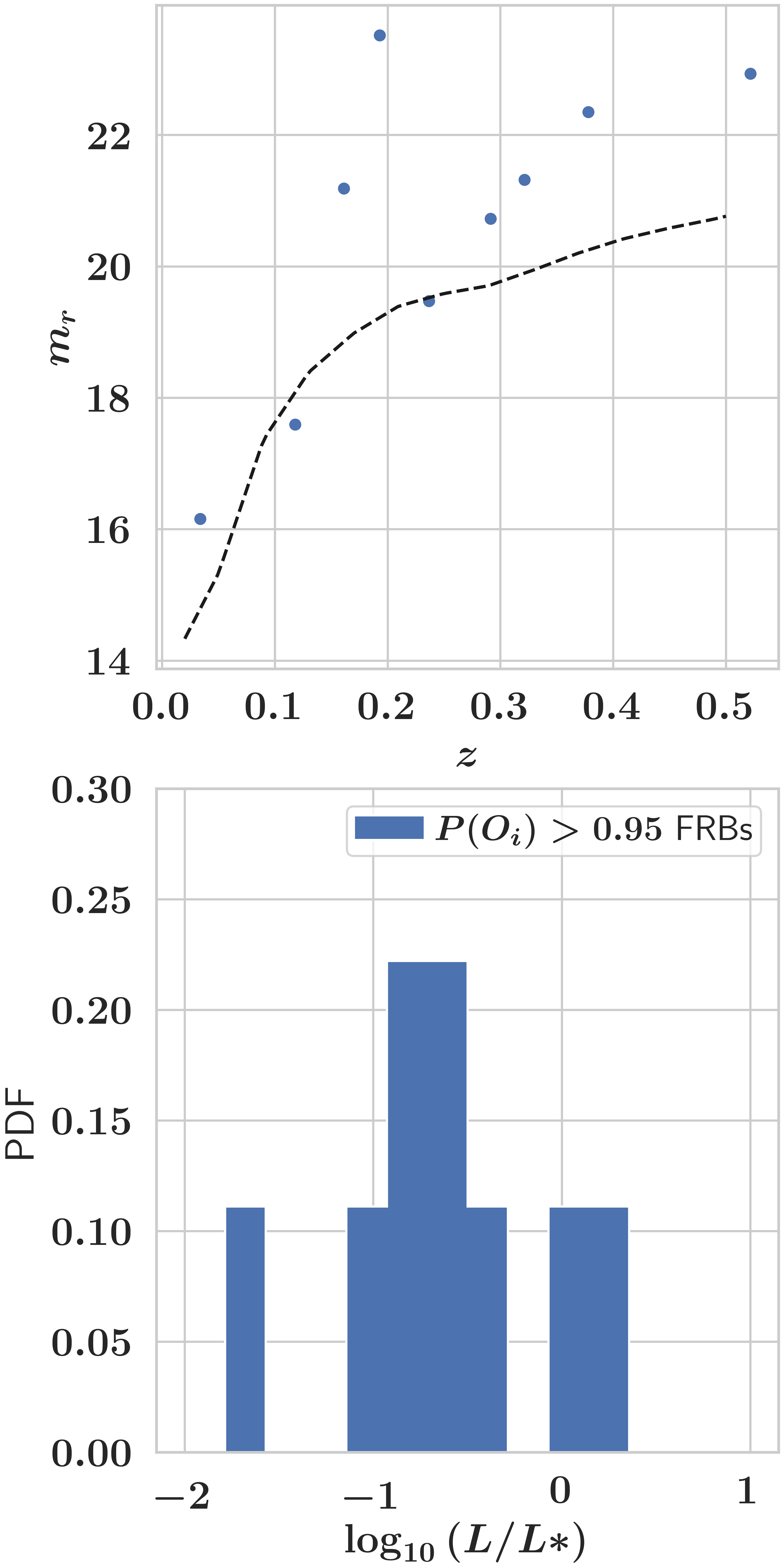
Figure 12: (top) Scatter plot of apparent magnitudes versus redshift for the nine host galaxies. These show an expected decrease in flux with increasing distance. The dashed line marks the approximate apparent magnitude for an $L*$ galaxy. (bottom) Estimated galaxy luminosity relative to the characteristic luminosity $L*$ at the host redshift. The secure hosts have a median $L/L*\approx 1/4$ and an RMS scatter of 0.5 dex.

Encoded in every FRB is its dispersion measure (DM), the path integral of free electrons along the sightline weighted by the cosmological scale factor. The first $\approx 10$ FRBs localized have established a firm correlation between DM and redshift, now termed the Macquart Relation (Macquart et al., 2020). This relation derives from the ionized plasma that permeates the cosmic web. Because redshift (i.e. distance) affects observed properties, one should consider incorporating the DM into the association analysis. A full and proper treatment, however, requires including the intrinsic luminosities and spectral slopes of FRBs convolved with instrumental sensitivity and even the triggering software (James et al., in prep.). Further, we emphasize that adopting the Macquart Relation as a prior would likely require estimating the redshift for every galaxy candidate; this will be intractable for many FRBs.

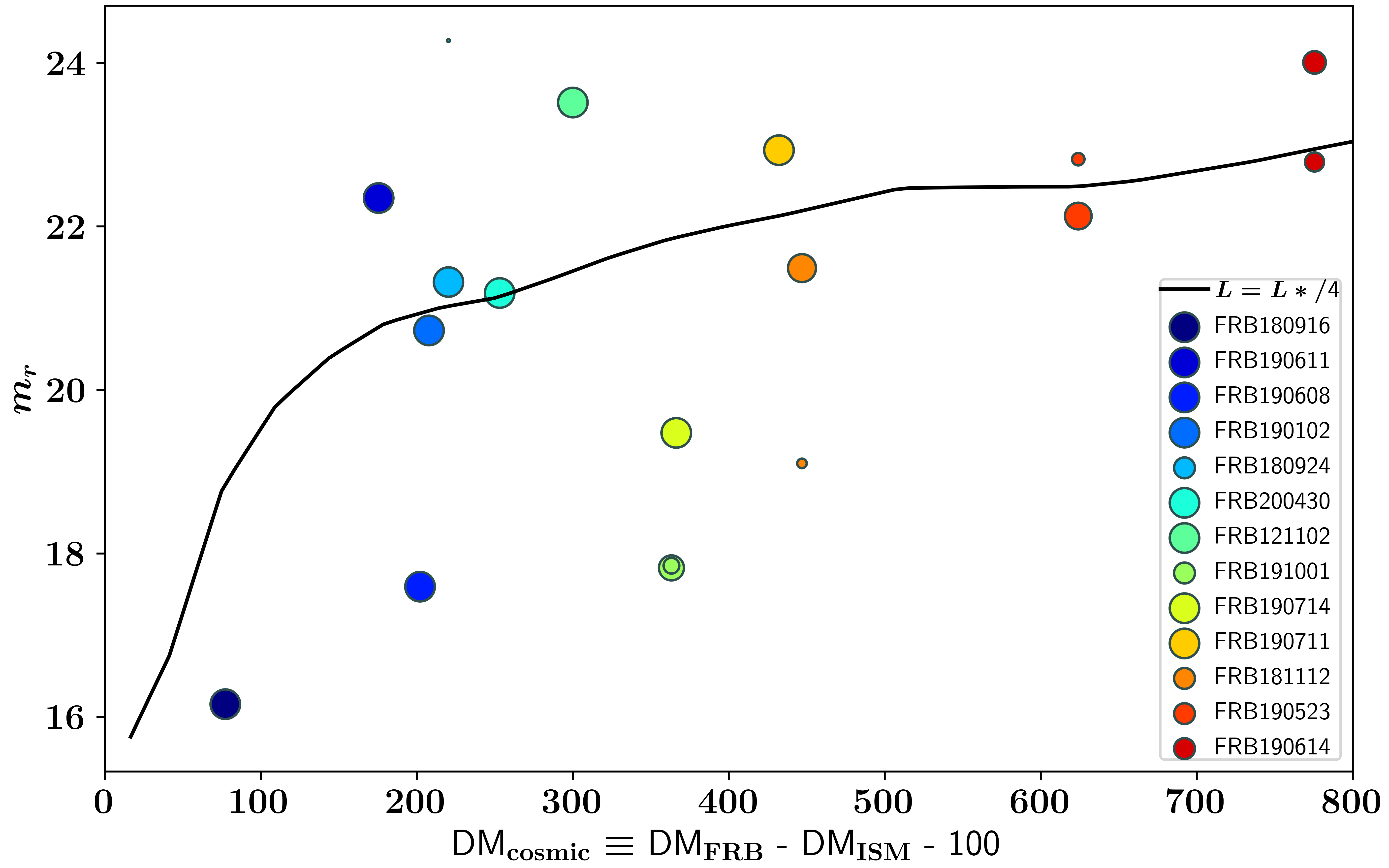
Figure 13: Using the adopted prior set (Table 3), we show the apparent magnitudes of each candidate with $P(O_{i}|x)>0.01$ scaling the point-size by $P(O_{i}|x)$. These are plotted against ${\rm DM}_{\rm cosmic}$, an estimate of the dispersion measure of the FRB due to the cosmic web (see text for details). The black curve shows the estimated $m_{r}$ for an $L=L*/4$ galaxy by converting ${\rm DM}_{\rm cosmic}$ to redshift (using the Macquart relation). The fact that the $m_{r}$ values track this curve implies an underlying Macquart relation.

In lieu of a direct application of the Macquart relation, we propose to leverage the luminosity distribution (Figure 12) together with DM. Figure 13 presents the apparent magnitudes of each galaxy candidate against an estimate of the cosmic dispersion measure ${\rm DM}_{\rm cosmic}$ with the point-size proportional to $P(O_{i}|x)$. For ${\rm DM}_{\rm cosmic}$, we adopt a simple estimation:

$${\rm DM}_{\rm cosmic}={\rm DM}_{\rm FRB}-{\rm DM}_{\rm MW,ISM}-100$$ (15)

with ${\rm DM}_{\rm MW,ISM}$ the estimated ISM dispersion measure (Cordes & Lazio, 2002) and the factor of 100 DM units accounts for the Galactic halo and the host galaxy (see Prochaska & Zheng, 2019; Macquart et al., 2020). The locus of data exhibits a clear correlation reflecting the decrease in observed galaxy flux with increasing distance.

Converting the ${\rm DM}_{\rm cosmic}$ estimates to redshift, we may convert a given $L_{r}$ luminosity to $m_{r}$; this is illustrated as the black curve in Figure 13 where we assumed a fiducial $L=L*/4$ based on Figure 12. The good correspondence between the data and this curve reveals the Macquart relation without having used any direct redshift measurements.

In principle, one could construct a prior $P(m_{r}|{\rm DM})$ to include in the analysis. This will, however, be subject to scatter in ${\rm DM}_{\rm cosmic}$ (Macquart et al., 2020), ${\rm DM}_{\rm host}$, and the intrinsic luminosities of the host galaxy population (Figure 12). It will also be subject, however, to the S/N considerations that affect any prior related to DM (James et al., 2020).

Table 5: Results for FRB Associations

FRB	RAcand	Deccand	$\theta$	$\phi$	$m$	Filter	$P^{c}$	$P(O)$	$P(O|x)$	$P(U)$	$P(U|x)$
Conservative
FRB121102	82.9945	$33.1479$	0.2	0.28	23.52	GMOS_N_i	0.0039	0.1000	1.0000	0.0000	0.0000
	82.9942	$33.1472$	2.9	0.28	21.14	GMOS_N_i	0.0113	0.1000	0.0000	0.0000	0.0000
	82.9935	$33.1473$	3.9	0.23	24.18	GMOS_N_i	0.2487	0.1000	0.0000	0.0000	0.0000
	82.9960	$33.1485$	4.7	0.25	23.28	GMOS_N_i	0.1818	0.1000	0.0000	0.0000	0.0000
	82.9939	$33.1492$	4.8	0.13	25.06	GMOS_N_i	0.5740	0.1000	0.0000	0.0000	0.0000
	82.9923	$33.1469$	7.9	0.28	21.58	GMOS_N_i	0.1169	0.1000	0.0000	0.0000	0.0000
	82.9968	$33.1490$	7.7	0.24	22.91	GMOS_N_i	0.3195	0.1000	0.0000	0.0000	0.0000
	82.9948	$33.1503$	8.5	0.15	24.95	GMOS_N_i	0.9101	0.1000	0.0000	0.0000	0.0000
	82.9918	$33.1470$	9.2	0.25	23.53	GMOS_N_i	0.6051	0.1000	0.0000	0.0000	0.0000
	82.9937	$33.1453$	10.0	0.31	20.19	GMOS_N_i	0.0501	0.1000	0.0000	0.0000	0.0000
FRB180916	29.5012	$65.7148$	7.7	3.03	16.16	GMOS_N_r	0.0005	0.0588	1.0000	0.0000	0.0000
	29.5054	$65.7140$	10.5	0.53	21.42	GMOS_N_r	0.1728	0.0588	0.0000	0.0000	0.0000
	29.5093	$65.7179$	10.0	0.21	22.00	GMOS_N_r	0.2554	0.0588	0.0000	0.0000	0.0000
	29.4998	$65.7130$	14.4	0.66	20.96	GMOS_N_r	0.2068	0.0588	0.0000	0.0000	0.0000
	29.5084	$65.7139$	12.7	0.24	22.71	GMOS_N_r	0.5888	0.0588	0.0000	0.0000	0.0000
	29.4913	$65.7174$	17.6	1.02	20.91	GMOS_N_r	0.2816	0.0588	0.0000	0.0000	0.0000
	29.5060	$65.7211$	16.3	0.41	21.29	GMOS_N_r	0.3312	0.0588	0.0000	0.0000	0.0000
	29.4996	$65.7203$	13.7	0.39	19.83	GMOS_N_r	0.0656	0.0588	0.0000	0.0000	0.0000
	29.5129	$65.7192$	17.1	0.37	20.03	GMOS_N_r	0.1202	0.0588	0.0000	0.0000	0.0000
	29.5136	$65.7181$	16.3	0.42	19.42	GMOS_N_r	0.0598	0.0588	0.0000	0.0000	0.0000
	29.5052	$65.7125$	15.7	0.43	18.15	GMOS_N_r	0.0141	0.0588	0.0000	0.0000	0.0000
	29.5122	$65.7171$	13.5	0.47	19.02	GMOS_N_r	0.0274	0.0588	0.0000	0.0000	0.0000
	29.5015	$65.7124$	15.7	0.16	21.13	GMOS_N_r	0.2748	0.0588	0.0000	0.0000	0.0000
	29.4933	$65.7138$	18.0	0.33	20.19	GMOS_N_r	0.1541	0.0588	0.0000	0.0000	0.0000
	29.5110	$65.7136$	16.4	0.19	22.17	GMOS_N_r	0.6012	0.0588	0.0000	0.0000	0.0000
	29.5021	$65.7130$	13.6	0.59	21.73	GMOS_N_r	0.3480	0.0588	0.0000	0.0000	0.0000
	29.5029	$65.7218$	18.3	0.28	21.64	GMOS_N_r	0.5053	0.0588	0.0000	0.0000	0.0000
FRB180924	326.1042	$-40.9002$	2.9	0.81	24.27	VLT_FORS2_g	0.1973	0.2500	0.7172	0.0000	0.0000
	326.1054	$-40.9002$	0.8	1.31	21.32	VLT_FORS2_g	0.0118	0.2500	0.2779	0.0000	0.0000
	326.1062	$-40.8993$	3.8	0.50	25.47	VLT_FORS2_g	0.5390	0.2500	0.0049	0.0000	0.0000
	326.1017	$-40.8998$	9.5	0.46	25.30	VLT_FORS2_g	0.9807	0.2500	0.0000	0.0000	0.0000
FRB181112	327.3486	$-52.9709$	0.4	0.67	21.49	VLT_FORS2_I	0.0227	0.2500	0.7588	0.0000	0.0000
	327.3496	$-52.9696$	5.4	1.06	19.10	VLT_FORS2_I	0.0073	0.2500	0.2411	0.0000	0.0000
	327.3484	$-52.9729$	7.0	0.58	22.01	VLT_FORS2_I	0.1646	0.2500	0.0001	0.0000	0.0000
	327.3467	$-52.9727$	7.4	0.32	24.05	VLT_FORS2_I	0.6612	0.2500	0.0000	0.0000	0.0000
FRB190102	322.4149	$-79.4756$	0.5	0.86	20.73	VLT_FORS2_I	0.0038	0.5000	1.0000	0.0000	0.0000
	322.4173	$-79.4773$	5.9	0.55	22.54	VLT_FORS2_I	0.1623	0.5000	0.0000	0.0000	0.0000
FRB190523	207.0642	$72.4706$	3.4	0.71	22.13	LRIS_R	0.1158	0.3333	0.6116	0.0000	0.0000
	207.0654	$72.4681$	5.8	0.61	22.82	LRIS_R	0.2986	0.3333	0.3712	0.0000	0.0000
	207.0589	$72.4691$	6.9	0.72	20.78	LRIS_R	0.0664	0.3333	0.0173	0.0000	0.0000
FRB190608	334.0203	$-7.8988$	2.5	1.66	17.60	VLT_FORS2_I	0.0005	0.2500	1.0000	0.0000	0.0000
	334.0185	$-7.8986$	5.0	0.30	24.83	VLT_FORS2_I	0.5373	0.2500	0.0000	0.0000	0.0000
	334.0186	$-7.8969$	6.6	0.26	25.28	VLT_FORS2_I	0.8461	0.2500	0.0000	0.0000	0.0000
	334.0187	$-7.8959$	9.5	0.45	22.76	VLT_FORS2_I	0.4081	0.2500	0.0000	0.0000	0.0000
FRB190611	320.7429	$-79.3973$	2.0	0.50	22.35	GMOS_S_i	0.0267	0.0909	0.9480	0.0000	0.0000
	320.7495	$-79.3972$	3.1	0.27	25.87	GMOS_S_i	0.5297	0.0909	0.0359	0.0000	0.0000
	320.7439	$-79.3985$	3.3	0.26	24.91	GMOS_S_i	0.3446	0.0909	0.0140	0.0000	0.0000
	320.7539	$-79.3979$	5.7	0.65	23.63	GMOS_S_i	0.3518	0.0909	0.0019	0.0000	0.0000
	320.7383	$-79.3977$	4.8	0.36	23.44	GMOS_S_i	0.2267	0.0909	0.0001	0.0000	0.0000
	320.7346	$-79.3988$	8.4	0.53	23.36	GMOS_S_i	0.5033	0.0909	0.0000	0.0000	0.0000
	320.7541	$-79.3965$	7.0	0.18	26.52	GMOS_S_i	0.9936	0.0909	0.0000	0.0000	0.0000
	320.7569	$-79.3991$	9.4	0.52	23.65	GMOS_S_i	0.6643	0.0909	0.0000	0.0000	0.0000
	320.7364	$-79.3998$	9.9	0.41	24.56	GMOS_S_i	0.9166	0.0909	0.0000	0.0000	0.0000
	320.7319	$-79.3970$	9.2	0.27	25.04	GMOS_S_i	0.9551	0.0909	0.0000	0.0000	0.0000
	320.7587	$-79.3986$	9.5	0.17	26.91	GMOS_S_i	1.0000	0.0909	0.0000	0.0000	0.0000
FRB190614	65.0743	$73.7068$	1.3	0.41	24.01	LRIS_I	0.0552	0.2000	0.6032	0.0000	0.0000
	65.0738	$73.7064$	2.2	0.40	22.79	LRIS_I	0.0386	0.2000	0.3968	0.0000	0.0000
	65.0705	$73.7075$	5.7	0.33	24.26	LRIS_I	0.4949	0.2000	0.0000	0.0000	0.0000
	65.0817	$73.7079$	7.5	0.17	26.35	LRIS_I	0.9945	0.2000	0.0000	0.0000	0.0000
	65.0691	$73.7081$	8.2	0.28	25.21	LRIS_I	0.9387	0.2000	0.0000	0.0000	0.0000
FRB190711	329.4194	$-80.3581$	0.5	0.46	22.93	GMOS_S_i	0.0108	0.2000	0.8821	0.0000	0.0000
	329.4187	$-80.3586$	2.1	0.26	24.88	GMOS_S_i	0.1471	0.2000	0.1179	0.0000	0.0000
	329.4143	$-80.3570$	4.7	0.22	24.69	GMOS_S_i	0.4654	0.2000	0.0000	0.0000	0.0000
	329.4117	$-80.3571$	5.7	0.29	24.88	GMOS_S_i	0.6545	0.2000	0.0000	0.0000	0.0000
	329.4190	$-80.3595$	5.3	0.25	23.97	GMOS_S_i	0.3682	0.2000	0.0000	0.0000	0.0000
FRB190714	183.9795	$-13.0212$	1.0	0.95	19.48	VLT_FORS2_I	0.0012	0.2000	1.0000	0.0000	0.0000
	183.9797	$-13.0193$	6.1	0.54	23.71	VLT_FORS2_I	0.3925	0.2000	0.0000	0.0000	0.0000
	183.9787	$-13.0229$	7.4	0.60	21.22	VLT_FORS2_I	0.0772	0.2000	0.0000	0.0000	0.0000
	183.9797	$-13.0230$	7.0	0.31	24.36	VLT_FORS2_I	0.6494	0.2000	0.0000	0.0000	0.0000
	183.9795	$-13.0234$	8.7	0.50	22.71	VLT_FORS2_I	0.3425	0.2000	0.0000	0.0000	0.0000
FRB191001	323.3525	$-54.7487$	3.9	1.36	17.82	VLT_FORS2_I	0.0009	0.3333	0.5412	0.0000	0.0000
	323.3492	$-54.7483$	5.3	1.47	17.85	VLT_FORS2_I	0.0015	0.3333	0.4588	0.0000	0.0000
	323.3501	$-54.7496$	7.3	0.27	25.11	VLT_FORS2_I	0.8690	0.3333	0.0000	0.0000	0.0000
FRB200430	229.7064	$12.3766$	0.9	0.72	21.19	LRIS_I	0.0056	0.5000	1.0000	0.0000	0.0000
	229.7088	$12.3778$	8.9	0.38	24.82	LRIS_I	0.9123	0.5000	0.0000	0.0000	0.0000
Adopted
FRB121102	82.9945	$33.1479$	0.2	0.28	23.52	GMOS_N_i	0.0039	0.0245	1.0000	0.0000	0.0000
	82.9942	$33.1472$	2.9	0.28	21.14	GMOS_N_i	0.0113	0.2026	0.0000	0.0000	0.0000
	82.9935	$33.1473$	3.9	0.23	24.18	GMOS_N_i	0.2487	0.0144	0.0000	0.0000	0.0000
	82.9960	$33.1485$	4.7	0.25	23.28	GMOS_N_i	0.1818	0.0298	0.0000	0.0000	0.0000
	82.9939	$33.1492$	4.8	0.13	25.06	GMOS_N_i	0.5740	0.0073	0.0000	0.0000	0.0000
	82.9923	$33.1469$	7.9	0.28	21.58	GMOS_N_i	0.1169	0.1332	0.0000	0.0000	0.0000
	82.9968	$33.1490$	7.7	0.24	22.91	GMOS_N_i	0.3195	0.0408	0.0000	0.0000	0.0000
	82.9948	$33.1503$	8.5	0.15	24.95	GMOS_N_i	0.9101	0.0079	0.0000	0.0000	0.0000
	82.9918	$33.1470$	9.2	0.25	23.53	GMOS_N_i	0.6051	0.0242	0.0000	0.0000	0.0000
	82.9937	$33.1453$	10.0	0.31	20.19	GMOS_N_i	0.0501	0.5152	0.0000	0.0000	0.0000
FRB180916	29.5012	$65.7148$	7.7	3.03	16.16	GMOS_N_r	0.0005	0.8200	1.0000	0.0000	0.0000
	29.5054	$65.7140$	10.5	0.53	21.42	GMOS_N_r	0.1728	0.0026	0.0000	0.0000	0.0000
	29.5093	$65.7179$	10.0	0.21	22.00	GMOS_N_r	0.2554	0.0015	0.0000	0.0000	0.0000
	29.4998	$65.7130$	14.4	0.66	20.96	GMOS_N_r	0.2068	0.0040	0.0000	0.0000	0.0000
	29.5084	$65.7139$	12.7	0.24	22.71	GMOS_N_r	0.5888	0.0008	0.0000	0.0000	0.0000
	29.4913	$65.7174$	17.6	1.02	20.91	GMOS_N_r	0.2816	0.0042	0.0000	0.0000	0.0000
	29.5060	$65.7211$	16.3	0.41	21.29	GMOS_N_r	0.3312	0.0029	0.0000	0.0000	0.0000
	29.4996	$65.7203$	13.7	0.39	19.83	GMOS_N_r	0.0656	0.0123	0.0000	0.0000	0.0000
	29.5129	$65.7192$	17.1	0.37	20.03	GMOS_N_r	0.1202	0.0101	0.0000	0.0000	0.0000
	29.5136	$65.7181$	16.3	0.42	19.42	GMOS_N_r	0.0598	0.0190	0.0000	0.0000	0.0000
	29.5052	$65.7125$	15.7	0.43	18.15	GMOS_N_r	0.0141	0.0763	0.0000	0.0000	0.0000
	29.5122	$65.7171$	13.5	0.47	19.02	GMOS_N_r	0.0274	0.0291	0.0000	0.0000	0.0000
	29.5015	$65.7124$	15.7	0.16	21.13	GMOS_N_r	0.2748	0.0034	0.0000	0.0000	0.0000
	29.4933	$65.7138$	18.0	0.33	20.19	GMOS_N_r	0.1541	0.0086	0.0000	0.0000	0.0000
	29.5110	$65.7136$	16.4	0.19	22.17	GMOS_N_r	0.6012	0.0013	0.0000	0.0000	0.0000
	29.5021	$65.7130$	13.6	0.59	21.73	GMOS_N_r	0.3480	0.0019	0.0000	0.0000	0.0000
	29.5029	$65.7218$	18.3	0.28	21.64	GMOS_N_r	0.5053	0.0021	0.0000	0.0000	0.0000
FRB180924	326.1054	$-40.9002$	0.8	1.31	21.32	VLT_FORS2_g	0.0118	0.8723	0.9889	0.0000	0.0000
	326.1042	$-40.9002$	2.9	0.81	24.27	VLT_FORS2_g	0.1973	0.0683	0.0111	0.0000	0.0000
	326.1062	$-40.8993$	3.8	0.50	25.47	VLT_FORS2_g	0.5390	0.0278	0.0000	0.0000	0.0000
	326.1017	$-40.8998$	9.5	0.46	25.30	VLT_FORS2_g	0.9807	0.0316	0.0000	0.0000	0.0000
FRB181112	327.3486	$-52.9709$	0.4	0.67	21.49	VLT_FORS2_I	0.0227	0.0784	0.8300	0.0000	0.0000
	327.3496	$-52.9696$	5.4	1.06	19.10	VLT_FORS2_I	0.0073	0.8646	0.1700	0.0000	0.0000
	327.3484	$-52.9729$	7.0	0.58	22.01	VLT_FORS2_I	0.1646	0.0484	0.0000	0.0000	0.0000
	327.3467	$-52.9727$	7.4	0.32	24.05	VLT_FORS2_I	0.6612	0.0086	0.0000	0.0000	0.0000
FRB190102	322.4149	$-79.4756$	0.5	0.86	20.73	VLT_FORS2_I	0.0038	0.8425	1.0000	0.0000	0.0000
	322.4173	$-79.4773$	5.9	0.55	22.54	VLT_FORS2_I	0.1623	0.1575	0.0000	0.0000	0.0000
FRB190523	207.0642	$72.4706$	3.4	0.71	22.13	LRIS_R	0.1158	0.1974	0.8153	0.0000	0.0000
	207.0654	$72.4681$	5.8	0.61	22.82	LRIS_R	0.2986	0.1070	0.1777	0.0000	0.0000
	207.0589	$72.4691$	6.9	0.72	20.78	LRIS_R	0.0664	0.6956	0.0070	0.0000	0.0000
FRB190608	334.0203	$-7.8988$	2.5	1.66	17.60	VLT_FORS2_I	0.0005	0.9930	1.0000	0.0000	0.0000
	334.0185	$-7.8986$	5.0	0.30	24.83	VLT_FORS2_I	0.5373	0.0010	0.0000	0.0000	0.0000
	334.0186	$-7.8969$	6.6	0.26	25.28	VLT_FORS2_I	0.8461	0.0007	0.0000	0.0000	0.0000
	334.0187	$-7.8959$	9.5	0.45	22.76	VLT_FORS2_I	0.4081	0.0053	0.0000	0.0000	0.0000
FRB190611	320.7429	$-79.3973$	2.0	0.50	22.35	GMOS_S_i	0.0267	0.3324	0.9990	0.0000	0.0000
	320.7495	$-79.3972$	3.1	0.27	25.87	GMOS_S_i	0.5297	0.0206	0.0006	0.0000	0.0000
	320.7439	$-79.3985$	3.3	0.26	24.91	GMOS_S_i	0.3446	0.0412	0.0004	0.0000	0.0000
	320.7539	$-79.3979$	5.7	0.65	23.63	GMOS_S_i	0.3518	0.1116	0.0001	0.0000	0.0000
	320.7383	$-79.3977$	4.8	0.36	23.44	GMOS_S_i	0.2267	0.1304	0.0000	0.0000	0.0000
	320.7346	$-79.3988$	8.4	0.53	23.36	GMOS_S_i	0.5033	0.1392	0.0000	0.0000	0.0000
	320.7541	$-79.3965$	7.0	0.18	26.52	GMOS_S_i	0.9936	0.0133	0.0000	0.0000	0.0000
	320.7569	$-79.3991$	9.4	0.52	23.65	GMOS_S_i	0.6643	0.1102	0.0000	0.0000	0.0000
	320.7364	$-79.3998$	9.9	0.41	24.56	GMOS_S_i	0.9166	0.0536	0.0000	0.0000	0.0000
	320.7319	$-79.3970$	9.2	0.27	25.04	GMOS_S_i	0.9551	0.0373	0.0000	0.0000	0.0000
	320.7587	$-79.3986$	9.5	0.17	26.91	GMOS_S_i	1.0000	0.0103	0.0000	0.0000	0.0000
FRB190614	65.0743	$73.7068$	1.3	0.41	24.01	LRIS_I	0.0552	0.1944	0.5825	0.0000	0.0000
	65.0738	$73.7064$	2.2	0.40	22.79	LRIS_I	0.0386	0.5335	0.4175	0.0000	0.0000
	65.0705	$73.7075$	5.7	0.33	24.26	LRIS_I	0.4949	0.1593	0.0000	0.0000	0.0000
	65.0817	$73.7079$	7.5	0.17	26.35	LRIS_I	0.9945	0.0350	0.0000	0.0000	0.0000
	65.0691	$73.7081$	8.2	0.28	25.21	LRIS_I	0.9387	0.0779	0.0000	0.0000	0.0000
FRB190711	329.4194	$-80.3581$	0.5	0.46	22.93	GMOS_S_i	0.0108	0.4782	0.9995	0.0000	0.0000
	329.4187	$-80.3586$	2.1	0.26	24.88	GMOS_S_i	0.1471	0.1010	0.0005	0.0000	0.0000
	329.4143	$-80.3570$	4.7	0.22	24.69	GMOS_S_i	0.4654	0.1163	0.0000	0.0000	0.0000
	329.4117	$-80.3571$	5.7	0.29	24.88	GMOS_S_i	0.6545	0.1010	0.0000	0.0000	0.0000
	329.4190	$-80.3595$	5.3	0.25	23.97	GMOS_S_i	0.3682	0.2036	0.0000	0.0000	0.0000
FRB190714	183.9795	$-13.0212$	1.0	0.95	19.48	VLT_FORS2_I	0.0012	0.7998	1.0000	0.0000	0.0000
	183.9797	$-13.0193$	6.1	0.54	23.71	VLT_FORS2_I	0.3925	0.0156	0.0000	0.0000	0.0000
	183.9787	$-13.0229$	7.4	0.60	21.22	VLT_FORS2_I	0.0772	0.1393	0.0000	0.0000	0.0000
	183.9797	$-13.0230$	7.0	0.31	24.36	VLT_FORS2_I	0.6494	0.0093	0.0000	0.0000	0.0000
	183.9795	$-13.0234$	8.7	0.50	22.71	VLT_FORS2_I	0.3425	0.0361	0.0000	0.0000	0.0000
FRB191001	323.3525	$-54.7487$	3.9	1.36	17.82	VLT_FORS2_I	0.0009	0.5074	0.7174	0.0000	0.0000
	323.3492	$-54.7483$	5.3	1.47	17.85	VLT_FORS2_I	0.0015	0.4920	0.2826	0.0000	0.0000
	323.3501	$-54.7496$	7.3	0.27	25.11	VLT_FORS2_I	0.8690	0.0005	0.0000	0.0000	0.0000
FRB200430	229.7064	$12.3766$	0.9	0.72	21.19	LRIS_I	0.0056	0.9566	1.0000	0.0000	0.0000
	229.7088	$12.3778$	8.9	0.38	24.82	LRIS_I	0.9123	0.0434	0.0000	0.0000	0.0000

7 Future Directions and Analyses

This paper and the accompanying code base provide a new methodology to make probabilistic associations of transients to hosts (PATH). While we were motivated by FRB science, the general framework is agnostic to transient type. Therefore, we anticipate it will be applied to GRBs, GW events, Type Ia SNe, and many other transients. We stress further that because it is fully probabilistic, the outputs may be coupled to other likelihood frameworks developed to constrain, e.g. progenitor models or cosmology.

Applied to 13 well-localised FRBs, our results identify nine secure host galaxies, with posterior probabilities $>0.95$ of being the true host. We have shown using a suite of ‘sandbox’ simulations that this identification is reliable under a wide range of true FRB host galaxy distributions. This allows a reliable data set to be used when analysing host galaxy properties, or using FRBs for cosmology. Furthermore, by assigning a quantitative probability to individual hosts, we allow even non-secure hosts associations to be used for statistical purposes, with appropriate weighting.

Using these data-sets, we tentatively identify relations between FRB DMs, and host galaxy redshifts, magnitudes, and luminosities. Our results disfavour FRBs as having large offsets from their host galaxies, and we exclude more than one FRB considered as having an unseen host ($p\lesssim 0.01$). Thus we can conclusively answer the oft-asked question “could the true host galaxies be missed?” with a “no”.

Regarding FRBs, future work will include: (i) leveraging the next set of $\sim 10$ FRBs to further refine the priors and offset function; and (ii) expanding the formalism to include additional observables (see the Appendix). The latter may require obtaining additional data or performing additional analyses (e.g. photo-$z$ estimates) than the simple flux and angular sizes considered here. One may also introduce and test priors motivated by progenitor models. Last, the analysis can inform observing strategies to optimize the probability of a secure association as a function of anticipated FRB redshift, localization error, and imaging quality.

References

- Bannister et al. (2019) Bannister, K. W., Deller, A. T., Phillips, C., et al. 2019, Science, 365, 565, doi: 10.1126/science.aaw5903
- Bhandari et al. (2020a) Bhandari, S., Sadler, E. M., Prochaska, J. X., et al. 2020a, ApJ, 895, L37, doi: 10.3847/2041-8213/ab672e
- Bhandari et al. (2020b) Bhandari, S., Bannister, K. W., Lenc, E., et al. 2020b, ApJ, 901, L20, doi: 10.3847/2041-8213/abb462
- Blanchard et al. (2016) Blanchard, P. K., Berger, E., & Fong, W.-f. 2016, ApJ, 817, 144, doi: 10.3847/0004-637X/817/2/144
- Blondin & Tonry (2007) Blondin, S., & Tonry, J. L. 2007, ApJ, 666, 1024, doi: 10.1086/520494
- Bloom et al. (2002) Bloom, J. S., Kulkarni, S. R., & Djorgovski, S. G. 2002, AJ, 123, 1111, doi: 10.1086/338893
- Budavári & Loredo (2015) Budavári, T., & Loredo, T. J. 2015, Annual Review of Statistics and Its Application, 2, 113–139, doi: 10.1146/annurev-statistics-010814-020231
- Budavári & Szalay (2008) Budavári, T., & Szalay, A. S. 2008, The Astrophysical Journal, 679, 301–309, doi: 10.1086/587156
- Cordes & Chatterjee (2019) Cordes, J. M., & Chatterjee, S. 2019, ARA&A, 57, 417, doi: 10.1146/annurev-astro-091918-104501
- Cordes & Lazio (2002) Cordes, J. M., & Lazio, T. J. W. 2002, arXiv e-prints, astro. https://arxiv.org/abs/astro-ph/0207156
- Day et al. (2020) Day, C. K., Deller, A. T., Shannon, R. M., et al. 2020, MNRAS, 497, 3335, doi: 10.1093/mnras/staa2138
- Driver et al. (2016) Driver, S. P., Wright, A. H., Andrews, S. K., et al. 2016, MNRAS, 455, 3911, doi: 10.1093/mnras/stv2505
- Eftekhari & Berger (2017) Eftekhari, T., & Berger, E. 2017, ApJ, 849, 162, doi: 10.3847/1538-4357/aa90b9
- Fishman & Meegan (1995) Fishman, G. J., & Meegan, C. A. 1995, Annual Review of Astronomy and Astrophysics, 33, 415, doi: 10.1146/annurev.aa.33.090195.002215
- Fong & Berger (2013) Fong, W., & Berger, E. 2013, ApJ, 776, 18, doi: 10.1088/0004-637X/776/1/18
- Fong et al. (2010) Fong, W., Berger, E., & Fox, D. B. 2010, ApJ, 708, 9, doi: 10.1088/0004-637X/708/1/9
- Fynbo et al. (2009) Fynbo, J. P. U., Jakobsson, P., Prochaska, J. X., et al. 2009, ApJS, 185, 526, doi: 10.1088/0067-0049/185/2/526
- Gal-Yam (2019) Gal-Yam, A. 2019, Annual Review of Astronomy and Astrophysics, 57, 305, doi: 10.1146/annurev-astro-081817-051819
- Heintz et al. (2020) Heintz, K. E., Prochaska, J. X., Simha, S., et al. 2020, ApJ, 903, 152, doi: 10.3847/1538-4357/abb6fb
- James et al. (2020) James, C. W., Osłowski, S., Flynn, C., et al. 2020, MNRAS, 495, 2416, doi: 10.1093/mnras/staa1361
- Law et al. (2020) Law, C. J., Butler, B. J., Prochaska, J. X., et al. 2020, ApJ, 899, 161, doi: 10.3847/1538-4357/aba4ac
- Lorimer et al. (2007) Lorimer, D. R., Bailes, M., McLaughlin, M. A., Narkevic, D. J., & Crawford, F. 2007, Science, 318, 777, doi: 10.1126/science.1147532
- Lunnan et al. (2015) Lunnan, R., Chornock, R., Berger, E., et al. 2015, ApJ, 804, 90, doi: 10.1088/0004-637X/804/2/90
- Macquart et al. (2020) Macquart, J. P., Prochaska, J. X., McQuinn, M., et al. 2020, Nature, 581, 391, doi: 10.1038/s41586-020-2300-2
- Marcote et al. (2020) Marcote, B., Nimmo, K., Hessels, J. W. T., et al. 2020, Nature, 577, 190, doi: 10.1038/s41586-019-1866-z
- McQuinn (2014) McQuinn, M. 2014, ApJ, 780, L33, doi: 10.1088/2041-8205/780/2/L33
- Planck Collaboration et al. (2016) Planck Collaboration, Ade, P. A. R., Aghanim, N., et al. 2016, A&A, 594, A13, doi: 10.1051/0004-6361/201525830
- Prochaska & Zheng (2019) Prochaska, J. X., & Zheng, Y. 2019, MNRAS, 485, 648, doi: 10.1093/mnras/stz261
- Prochaska et al. (2019) Prochaska, J. X., Macquart, J.-P., McQuinn, M., et al. 2019, Science, 366, 231, doi: 10.1126/science.aay0073
- Ravi et al. (2019) Ravi, V., Catha, M., D’Addario, L., et al. 2019, Nature, 572, 352, doi: 10.1038/s41586-019-1389-7
- Scoville et al. (2007a) Scoville, N., Abraham, R. G., Aussel, H., et al. 2007a, ApJS, 172, 38, doi: 10.1086/516580
- Scoville et al. (2007b) Scoville, N., Aussel, H., Brusa, M., et al. 2007b, ApJS, 172, 1, doi: 10.1086/516585
- Tendulkar et al. (2017) Tendulkar, S. P., Bassa, C. G., Cordes, J. M., et al. 2017, ApJ, 834, L7, doi: 10.3847/2041-8213/834/2/L7
- Tunnicliffe et al. (2014) Tunnicliffe, R. L., Levan, A. J., Tanvir, N. R., et al. 2014, MNRAS, 437, 1495, doi: 10.1093/mnras/stt1975